| I. Macroeconomic Outlook The inflation outlook for 2016-17 has improved, but beyond, close vigilance is required to achieve the prospects of reaching 4 per cent i.e., the centre of the target band. Robust consumption brightens the outlook for real gross value added (GVA) in 2016-17, but muted private investment and weak global demand may restrain the pace of growth in 2017-18. Amendments to the Reserve Bank of India (RBI) Act, which came into force on June 27, 2016 will empower the conduct of monetary policy in India. For the first time in its history, the RBI has been explicitly provided the legislative mandate to operate the monetary policy framework of the country. The primary objective of monetary policy has also been defined explicitly for the first time – “to maintain price stability while keeping in mind the objective of growth.” The amendments also provide for the constitution of a monetary policy committee (MPC) that shall determine the policy rate required to achieve the Inflation target, another landmark in India’s monetary history. The composition of the MPC, terms of appointment, information flows and other procedural requirements such as implementation of and publication of its decisions, and failure to maintain the Inflation target as well as remedial actions have been specified and subsequently gazetted. On August 5, 2016 the Government set out the Inflation target as four per cent with upper and lower tolerance levels of six per cent and two per cent, respectively. The Government and the RBI have constituted the six member MPC. All conditions are, therefore, in place for the MPC to take its first decision on October 4 under the Reserve Bank’s fourth bi-monthly monetary policy review for 2016-17. The amended RBI Act establishes the procedures for MPC meetings. It specifically lays down that the Bank shall organise at least four meetings of the MPC in a year (Section 45ZI). The cross-country experience in this regard is varied, both in terms of the number of meetings and the press conferences that usually follow the meetings in order to explain the stance of monetary policy for the benefit of the public. A survey of country practices suggests a central tendency among major central banks to hold four press conferences a year, although the number of MPC meetings may be higher (Table I.1). | Table I.1: Monetary Policy Meetings and Press Conferences | | Name of the Central Bank/ Monetary Authority | Number of Monetary Policy Meetings in a Year | Number of Press Conferences in a Year | | Bank of England | 8 | 4 (a) | | US Federal Reserve | 8 | 4 | | Bank of Canada | 8 | 4 | | Reserve Bank of New Zealand | 7 | 4 | | Bank of Israel | 12 | 4 | | | (8 from 2017) | | | Bank of Russia | 8 | 4 | | Central Bank of the Republic of Turkey | 12 | 4 (b) | | Bank Indonesia | 12 | 4 | | Banco Central Do Brasil | 8 | 4 (c) | | European Central Bank | 8 | 8 | | Norges Bank | 6 | 6 | | Bank of Japan | 8 | 8 | | Bank of Korea | 12 | 12 | | South African Reserve Bank | 6 | 6 | | Czech National Bank | 8 | 8 | Notes:
(a) : Inflation Report press conference.
(b) : Governor’s speech/presentation at the briefing on the Inflation Report.
(c) : Presentation by central bank director at the quarterly Inflation Report.
Source: Central Bank websites. | Chapters II and III compare Inflation and growth outcomes with the April 2016 forecasts and drill down into factors underlying deviations. Turning to the outlook, the April 2016 monetary policy report (MPR) presaged the continuing weakening of global growth and external demand. At the September G20 Summit in Hangzhou, the International Monetary Fund (IMF) warned about an even more modest pace of global growth this year, with the balance of risks remaining skewed to the downside (Chart I.1). This will necessitate an adjustment to assumptions on initial conditions for the projections given in this MPR. Furthermore, international crude oil prices, which fell to a recent trough in early April, have been edging up in ensuing months and the slightly firmer note in these prices observed since July will need to be factored into the assumptions (Table 1.2). 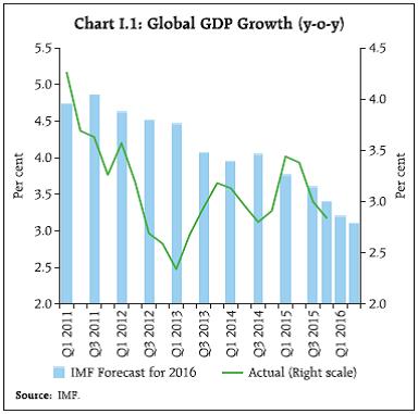
| Table I.2: Baseline Assumptions for Near-Term Projections | | Variable | April 2016 MPR | Current (October 2016) MPR | | Crude Oil (Indian Basket)* | US$ 40 per barrel during FY 2016-17 | US$ 46 per barrel during 2016-17:H2 | | Exchange rate ** | ₹68.5 per US$ | Current level | | Monsoon | Normal for 2016 | Normal for 2016 | | Global growth *** | 3.4 per cent in 2016 | 3.1 per cent in 2016 | | 3.6 per cent in 2017 | 3.4 per cent in 2017 | | Fiscal deficit | To remain within BE 2016-17 (3.5 per cent) | To remain within BE 2016-17 (3.5 per cent) | | Domestic macroeconomic/ structural policies during the forecast period | No major change | No major change | Notes:
* Represents a derived basket comprising sour grade (Oman and Dubai average) and sweet grade (Brent) crude oil processed in Indian refineries in the ratio of 71:29.
** The exchange rate path assumed here is for the purpose of generating staff’s baseline growth and inflation projections and does not indicate any ‘view’ on the level of the exchange rate. The Reserve Bank is guided by the need to contain volatility in the foreign exchange market and not by any specific level/ band around the exchange rate.
*** Based on projections from January 2016 and July 2016 Updates of the IMF’s World Economic Outlook. | International petroleum product price benchmarks used by domestic oil marketing companies (OMCs) to set domestic pump prices of petrol and diesel at fortnightly intervals tend to be highly correlated with international crude prices (0.9). On the other hand, domestic pump prices and international petroleum product prices diverge on account of refinery/maintenance/inventory costs and domestic tax structures, with this wedge having increased significantly since November 2014 in view of excise duty increases. Of every one per cent change in international product prices (lagged by a fortnight to simulate pump price revisions in India), only 0.31 per cent is reflected in domestic pump prices of petrol, the pass-through increasing to 0.42 per cent during episodes of international price increases and falling to 0.28 per cent during international price declines (Chart I.2; see also Chapter II). In 2016 so far, however, a substantially higher degree of pass-through is being observed. 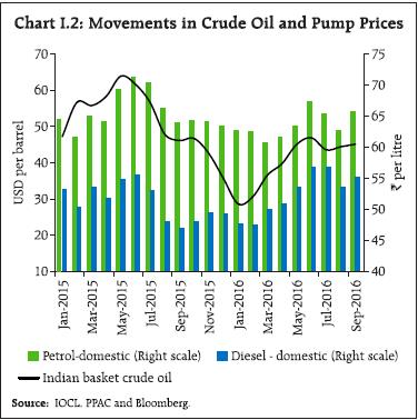 I.1 The Outlook for Inflation Daily price collections of sensitive items under pulses, fruits, vegetables and cereals suggest that the seasonal surge in food prices may have peaked in July. Subdued momentum in food Inflation in Q3 and the usual seasonal softening of food prices in early Q4, notwithstanding a reversal of base effects in March 2017, improves the near-term outlook for Inflation considerably. Commodity prices are expected to remain quiescent over the rest of the year. These anticipated developments feed into Inflation expectations and, in turn, influence wage and price conditions, going forward. Among various economic agents, households tend to be the most adaptive in their expectations formation. Accordingly, food price increases of May-July appear to have remained entrenched in their Inflation expectations. The September round of the Reserve Bank’s survey of urban households indicates a pick-up in their current perceptions and expectations of Inflation farther out, as in the June round of the survey, with an increase in the proportion of respondents expecting prices to rise by more than the current rate1 (Chart I.3). In the September round, in fact, Inflation is expected to be 9.5 per cent three months ahead and 11.4 per cent one year ahead. 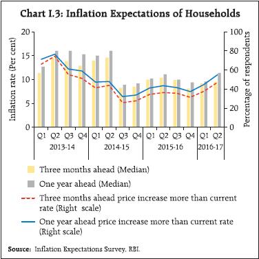 By contrast, producers’ Inflation expectations appear to be more forward-looking. The July-September round of the Reserve Bank’s industrial outlook survey2 reveals an increase in the proportion of respondents expecting higher input prices in Q3. The survey also indicates a decline in their expectations of higher selling prices (Chart I.4). Expectations of improvement in demand conditions should be comfortably absorbed by the presence of spare capacity. Manufacturing purchasing managers polled in Nikkei’s survey for September 2016 indicate that, despite some uptick, both input and output price indices were lower than their long-term averages. Increases in staff costs in the organised sector as well as nominal rural wage growth – especially with the deceleration in July – are expected to remain moderate in Q3. 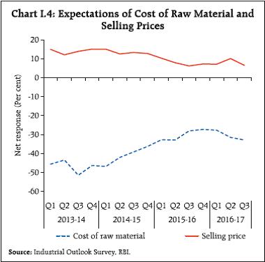 The September round of the Reserve Bank’s survey of professional forecasters indicates a greater degree of anchoring of their Inflation expectations, relative to other agents, around the Reserve Bank’s Inflation targets (Chart I.5). They expect Inflation to ease to 4.7 per cent by Q4 of 2016-17 and to 4.4 per cent by Q2 of 2017-18, both lying within the Reserve Bank’s Inflation target band. While their medium-term Inflation expectations (five years ahead) have remained unchanged at 5 per cent, their longer-term expectations (10 years ahead) have moved down to 4.5 per cent from 4.8 per cent polled in the immediately preceding round of the survey. These expectations reflect the stubborn persistence that may be encountered in moving below current levels of Inflation.  Staff’s baseline model forecasts, taking into account the revisions in assumptions on initial conditions and augmented by information yielded by these forward-looking surveys of various classes of economic agents as well as from lead indicators, set a trajectory that takes consumer price index (CPI) Inflation down from 5.7 per cent in Q1 of 2016-17 to 5.0 per cent in Q3 before it firms up moderately to 5.3 per cent in Q4 (the 70 per cent confidence interval lies in a range of 3.9-7.0 per cent) (Chart I.6). These projections incorporate the 7th pay commission’s award relating to salaries and pensions which will work through aggregate demand and expectations effects to add around 10 basis points (bps) to the baseline path from Q4 of 2016-17. Furthermore, the projections also factor in cost-push effects of the proposed increase in minimum wages which would add 5 bps to baseline Inflation within two months of implementation3. Taking into account these shocks to the baseline and given the initial conditions in Table I.2, staff projects Inflation to ease modestly through 2017-18 and reach 4.5 per cent by Q4 of 2017-18 (2.1 per cent to 7.7 per cent defining the 70 per cent confidence interval). By current reckoning, the pass-through of the goods and services tax (GST) will likely commence from April 2017 and last for about 12-18 months, going by the cross-country experience. While the impact of the GST on CPI Inflation would largely depend on the standard rate decided by the GST Council, almost 50 per cent of the CPI is expected to be exempt. Cross-country experience indicates that the GST implementation might have one-off effects, which tend to dissipate after a year of its implementation (see Chapter II). It is in the context of unanticipated shocks to the future evolution of Inflation that the rationale of setting India’s Inflation target at 4 per cent with a tolerance band of +/- 2 per cent can be appreciated. Globally too, the subject of the appropriate level of the Inflation target is being intensely debated. For advanced economies, the wide-spread practice of a 2 per cent Inflation target has come under considerable scrutiny in the aftermath of the global financial crisis. The crisis showed that large adverse shocks can and do happen and when they do, policymakers need room for monetary policy to react to them, especially when the longer-term prospects of the economy are jeopardised. Accordingly, a view has been expressed that they should aim for a higher Inflation target of say 4 per cent since the costs of Inflation at 4 per cent and/or of anchoring expectations at 4 per cent are judged to be lower than the benefits of headroom made available to monetary policy to stabilise the economy in the face of recession risks. More recently, the potential benefits of a higher Inflation target have been cited in the context of the secular decline in the natural/neutral rate of interest (Williams, 20164)5. I.2 The Outlook for Growth The April 2016 MPR had outlined the key downside risks that could impinge upon the path of growth in 2016-17 – the depressed private investment climate amidst subdued capacity utilisation and corporate balance sheet deleveraging; depressed global output and trade growth dragging down net exports. It also highlighted several positive factors that could potentially lift growth, including the government’s “start-up” and other initiatives, the boost to household consumption demand from the 7th Central Pay Commission (CPC) award, still benign cost conditions, measures announced in the Union Budget 2016- 17 to transform the rural sector, upbeat consumer confidence and the expected recovery in agriculture and allied activities. Since then, some of these assumptions have materialised. Accordingly, the spatially and temporally satisfactory south-west monsoon during the 2016 season, and the implementation of the 7th CPC award are expected to provide a boost to consumption spending, both rural and urban. The Reserve Bank’s survey conducted in August-September 2016 found consumer optimism on the general economic outlook, but somewhat less confidence on future income and employment6 (Chart I.7). While private investment activity remains sluggish, corporate business expectations remain upbeat in the Reserve Bank’s industrial outlook survey on improving prospects for production, capacity utilisation, employment and the availability of finance (Chart I.8). This positive sentiment was also reflected in business confidence surveys conducted by other institutions (Table I.3).
| Table I.3: Business Expectations Surveys | | Item | NCAER Business Confidence Index | FICCI Overall Business Confidence Index | Dun and Bradstreet Composite Business Optimism Index | CII Business Confidence Index | | Q1: 2016-17 | June 2016 | Q3: 2016 | Q1: 2016-17 | | Current level of the index | 124.3 | 64.3 | 83.2 | 57.2 | | Index as per previous Survey | 121.6 | 56.7 | 81.1 | 54.1 | | % change (q-o-q) sequential | 2.2 | 13.4 | 2.6 | 5.7 | | % change (y-o-y) | 2.1 | -3.0* | 6.7 | 5.1 | | *: Variation over August 2015 survey. | Over the medium-term, the implementation of the GST should boost business confidence and investment, brightening the environment for an acceleration of growth. Other initiatives such as steps to attract foreign direct investment in defence, civil aviation, pharmaceuticals and broadcasting, measures to improve infrastructure, and the enactment of the Insolvency and Bankruptcy Code and the Real Estate (Regulation and Development) Act should also contribute to unlocking entrepreneurial energies and growth impulses. Professional forecasters surveyed during September 2016 expected real GVA growth to improve from 7.3 per cent in 2016-17:Q1 to 7.6 per cent each in the remaining three quarters of 2016-17 on account of better agricultural prospects (Chart I.9 and Table I.4). 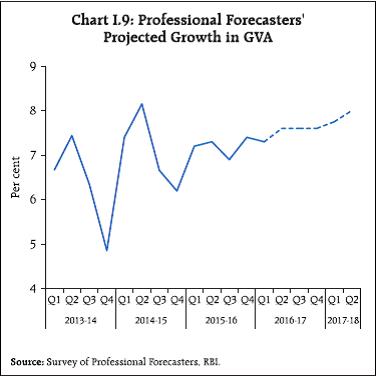
| Table I.4: Reserve Bank's Baseline and Professional Forecasters' Median Projections | | (Per cent) | | | 2016-17 | 2017-18 | | Reserve Bank’s Baseline Projections | | Inflation, Q4 (y-o-y) | 5.3 | 4.5 | | Real Gross Value Added (GVA) Growth | 7.6 | 7.9 | | Assessment of Survey of Professional Forecasters@ | | GVA Growth | 7.6 | 7.8 | | Agriculture and Allied Activities | 3.5 | 3.0 | | Industry | 7.5 | 7.9 | | Services | 8.8 | 9.2 | | Inflation, Q4 (y-o-y) | 4.7 | 4.4 # | | Gross Domestic Saving (per cent of GNDI) | 31.6 | 32.1 | | Gross Fixed Capital Formation (per cent of GDP) | 29.5 | 29.8 | | Money Supply (M3) Growth | 11.5 | 12.3 | | Credit Growth of Scheduled Commercial Banks | 11.5 | 13.0 | | Combined Gross Fiscal Deficit (per cent of GDP) | 6.5 | 6.0 | | Central Government Gross Fiscal Deficit (per cent of GDP) | 3.5 | 3.3 | | Repo Rate (end period) | 6.25 | 6.25 | | CRR (end period) | 4.00 | 4.00 | | Yield of 91-Days Treasury Bills (end period) | 6.4 | 6.4 | | Yield of 10-years Central Government Securities (end period) | 6.8 | 6.8 | | Overall Balance of Payments (US$ bn.) | 24.7 | 34.0 | | Merchandise Exports Growth | 1.2 | 6.1 | | Merchandise Imports Growth | -1.1 | 9.2 | | Merchandise Trade Balance (per cent of GDP) | -6.0 | -5.6 | | Current Account Balance (per cent of GDP) | -1.0 | -1.2 | | Capital Account Balance (per cent of GDP) | 2.0 | 2.9 | @: Median forecasts. #: Q2: 2017-18
GNDI: Gross National Disposable Income.
Source: Survey of Professional Forecasters (September 2016). | Taking into account these developments in conjunction with signals from various surveys and indicators and updated model forecasts, staff retains the projection of real GVA growth at 7.6 per cent for 2016-17, with a range of 7.6-7.7 per cent in Q2-Q4 (Chart I.10). For 2017-18, assuming a normal monsoon, fiscal consolidation in line with the announced trajectory and no major exogenous/policy shock(s), structural model estimates and off-model adjustments (Box I.1), real GVA growth of 7.9 per cent indicated in April is retained, but with downside risks mainly due to lower global demand vis-à-vis the April MPR. Box I.1: Nowcasting Economic Activity It is widely accepted that monetary policy needs to be forward-looking and should respond to expectations, since it affects Inflation and output with varying lags. Moreover, lags in data releases challenge the assessment of underlying economic conditions. Illustratively, the latest data on GDP, which became available on August 31, 2016 pertain to April-June 2016; GDP data for the quarter July-September 2016 – the quarter that is most relevant to this MPR as a starting point – will be released at the end of November 2016. Therefore, timely and accurate projections of these key goal variables are important. As noted in the MPR of September 2015, the Reserve Bank deploys a host of modelling approaches for generating forecasts. It also scans a host of incoming data to “nowcast” the current state of the economy. The “nowcasting” process involves analysing a number of leading and concurrent indicators of economic activity through a dynamic factor model (DFM) to estimate GVA growth for the relevant quarter, as well as the immediately preceding and following quarters. With an initial input of around 47 variables, the DFM exploits the co-movement among the series to select a relatively few salient ‘factors’. Given that data releases are scattered over the course of a month, the nowcast is updated as soon as new information comes in, thus providing an assessment of the economy almost in real time. The nowcasting of India’s GVA employs not only coincident and lead indicators but also survey results. Chart A presents nowcasts at the end of the relevant quarter - for example, the nowcast for the quarter January-March 2016 is based on information up to end-March. Chart B evaluates nowcasting performance over alternative horizons (from 2 months before the end of the reference quarter to one month after the reference quarter), and indicates an improvement in model performance as more information becomes available. The model performs better than a benchmark random walk (RW) model. Nonetheless, there are formidable challenges to nowcasting performance from the data – the persisting wide wedge between growth in industrial production and the growth in GVA in the manufacturing sector necessitates off-model adjustments to the results.
Reference: Giannone, Domenico, Lucrezia Reichlin and David Small (2008), “Nowcasting: The Real-time Informational Content of Macroeconomic Data”, Journal of Monetary Economics, Vol. 55, pp.665-676. I.3 Balance of Risks (i) Implementation of the 7th Central Pay Commission Award on Allowances While the second round impact of the 7th CPC award in the form of salaries and pensions is incorporated in the baseline forecasts, the effect of house rent allowances (HRA) is not, since its implementation was deferred, pending a review. As and when the revised allowances are awarded, they will have a direct impact on headline CPI Inflation through an increase in housing Inflation (house rents have a weight of 9.5 per cent in the CPI). In addition, indirect effects could arise through Inflation expectations. Assuming that (a) the revised allowances are implemented from early 2017, (b) the increase proposed by the 7th CPC is retained7, and (c) state governments implement a similar order of increase in allowances with a lag of one quarter, headline CPI Inflation in 2017-18 could be 100-150 bps above the baseline. The impact on Inflation is expected to persist for 6-8 quarters, with the peak effect occurring at around 3-4 quarters following the implementation (Chart I.11). While for policy purposes, the statistical direct effects of the increase in HRA should be looked through since they do not constitute an increase in true Inflation, model simulations indicate that indirect effects arising out of aggregate demand effects and rise in Inflation expectations may require a tightening of the monetary policy stance to ensure that Inflationary pressures from this factor do not get generalised and entrenched into expectations. 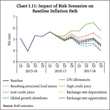 (ii) Moderation in Pulses Inflation A striking characteristic of food Inflation in recent years has been its persistence in certain groups such as pulses. In turn, this characteristic imparts stickiness to overall Inflation formation. Pulses, which have a weight of just 2.4 per cent in the CPI, have accounted for around 12-20 per cent of overall Inflation since mid-2015, manifesting structural demand supply imbalances rather than transient mismatches. Several initiatives have been undertaken over the past year to augment supply and bring down pulses Inflation (see Chapter II). If these efforts are able to bring down the prices of pulses on a sustained basis, food Inflation could ebb by around 35 bps by 2016-17:Q4 and around 100 bps by 2017-18:Q4 and, through a process of relative price adjustments, overall Inflation could moderate by 15 bps in 2016-17:Q4 and 50 bps by 2017-18:Q4. (iii) Exchange Rate Movements Uncertainty prevailing about the pace of US monetary policy normalisation tends to get amplified by every incoming data. The outcome of the US presidential election also adds to uncertainty. Consequently, spillovers purvey volatility to global and domestic financial markets, especially in the foreign exchange, equity and debt segments, with implications for domestic Inflation and growth. A five per cent depreciation of the Indian rupee vis-à-vis the US dollar could increase Inflation by 10-15 bps and real GVA growth by 5-10 bps above the baseline through effects on net exports (Charts I.11 and I.12). Model simulations that incorporate the resulting rise in headline Inflation above the baseline path and a faster closing of the output gap could indicate monetary policy tightening. 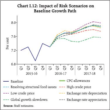 On the other hand, India could become a preferred destination of capital flows, as is the case currently, in view of relatively stronger macroeconomic fundamentals. This may cause the rupee to appreciate. An appreciation of the rupee by 5 per cent could moderate Inflation by around 10-15 bps and real GVA growth by 10 bps below the baseline. (iv) International Crude Oil Prices International crude oil prices have remained volatile in recent months. The price of the Indian basket increased from around US$ 36 per barrel in March 2016 to US$ 47 in July before softening again to around US$ 44 in August-September. Consequently, the baseline assumption in Table I.2 could be subject to variations on either side. If crude oil prices increase to US$ 70 per barrel by the end of 2017-18 (higher by around 40 per cent than the baseline assumption), Inflation could be higher by about 40-60 bps, while real GVA growth could weaken by around 20 bps relative to baseline paths by March 2018. Returning the goal variables to their baseline trajectories would require monetary policy tightening. On the other hand, crude prices could also soften below the baseline assumption in an event of weaker than expected global demand, and/or excess supply of crude in global markets. If crude oil prices fall to around US$ 35 per barrel and this softening is passed on to pump prices of petroleum products in India, Inflation may be about 30-50 bps below its baseline, while real GVA growth could be around 15 bps above its baseline. (v) Global Demand Stagnation Global growth has been muted so far and projections by various agencies for this year and the next are expected to downgrade the outlook for global growth even further. The uncertainty associated with the “Brexit”, the US presidential election and the still nebulous effects of US monetary policy normalisation and Chinese re-balancing, could undermine global economic activity even more. Should global growth be one percentage point below the assumed baseline, domestic real GVA growth and Inflation could be 20-40 bps and 10-20 bps below their respective baseline forecasts. The near-term outlook for the Indian economy is characterised by a continuing slow recovery, underpinned by consumption spending and by public investment at the margin. As regards Inflation, the outlook has improved for 2016-17, but beyond, the prospects of reaching 4 per cent i.e., the centre of the target band requires close monitoring. Recent initiatives and reforms by the government such as ‘Make in India’, measures to improve the infrastructure, the scheduled introduction of the GST, improvements in food supply management and steps to enhance domestic production of fertilisers as well as a reduction in prices of non-urea fertilisers are expected to help disinflate in the medium-term. Even as the urgency of safeguarding near-term growth and stability has increased, the policy challenge is to bolster medium-term growth prospects through structural reforms that step up new investment in the economy on a sustained basis, renew skills and job creation, and broaden the swathe of the growth process to include the widest sections of society in its benefits. Globally, the danger of secular stagnation and an entrenchment of lastingly impaired potential output have become more tangible than before. Besides the main priority of lifting both actual and potential output, keeping financial stability risks in check, containing external vulnerabilities, and building resilience is essential if an adjustment to diminished growth prospects globally becomes inevitable.
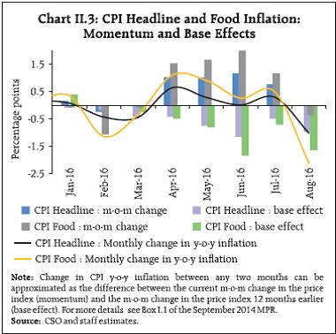
II. Prices and Costs Consumer price inflation was pushed up by a surge in the momentum of food inflation during April-July 2016 before a sharp correction set in during August. Input costs firmed up moderately for both farm and non-farm sectors alongside corporate staff costs. Drawing on a modest softening of households’ and professional forecasters’ Inflation expectations, still muted corporate pricing power and model forecasts, the April 2016 MPR envisaged a trajectory on which headline CPI Inflation1 would edge down from 5.4 per cent in Q4 of 2015-16 to 5.3 per cent in Q1 of 2016-17 and to 5.1 per cent in Q2. In the event, the momentum of the seasonal firming up of food prices that usually sets in from April was much stronger than anticipated, especially in vegetables prices. Moreover, occurring as it did on top of highly elevated prices of pulses, it imparted an unusual upside to Inflation that lasted right up to July. In addition, international crude prices rose from a recent trough in April to US$ 44 per barrel by September. Crude prices averaged US$ 44 per barrel during April-September as against US$ 40 per barrel in the assumptions on initial conditions in the April 2016 MPR. Consequently, headline CPI Inflation averaged higher at 5.7 per cent in Q1 of 2016-17, deviating from the forecast of 5.3 per cent (Chart II.1). With the rapid waning of these transient price pressures in August, Inflation momentum collapsed. Inflation appears to be returning to the April 2016 forecast path, albeit from some elevation. A one percentage point deviation of food Inflation from its trajectory projected in the April MPR leads to 47 basis points increase in headline Inflation in terms of the direct effect alone and this perturbation could cause headline Inflation to diverge from its projected path for upto four to six months, based on impulse responses in an unrestricted vector autoregression (VAR) framework. This imparts a modest potential upside to the balance of risks around the target of 5 per cent for Q4 of 2016-17. II.1 Consumer Prices The April 2016 projections were predicated on the presence of favourable base effects arising from high Inflation a year ago, with the base effects for food Inflation stronger than those pulling down the headline. Even while the downside base effects were significant up to June-July, they were overwhelmed by a surge in the month-on-month (m-o-m) momentum – especially of food prices – which peaked in July. As surprisingly as it took hold, the momentum of headline CPI dissipated completely in August, with the momentum of food prices turning negative. With this unexpected reversal, sizable base effects in that month came into full play and pulled down overall Inflation to 5.05 per cent, an intra-year low, in August (Charts II.2 and II.3). 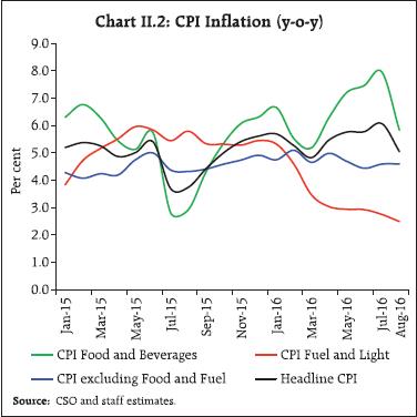
 The transient upsurge in Inflation momentum in April-July was induced by two main drivers – pulses and vegetables – as evident in the strong positive skew of the distribution of Inflation (Chart II.4). This is corroborated by a significant fall in the diffusion index of price changes in CPI during the first half of 2016-17, which suggests that Inflationary impulses were confined to a few food items (Chart II.5).
II.2 Drivers of Inflation In a forward-looking perspective, Inflation developments are likely to be influenced by three domestic drivers which, in themselves, embed upside risks to the Inflation target, namely (a) spatial distribution of food Inflation pressures; (b) the implementation of the 7th CPC award, especially house rent allowances and subsequently, implementation by states; and (c) the 42 per cent increase in minimum wages across the board for the central sphere2. Accordingly, the narrative in the rest of this chapter, albeit backward-looking, will be tilted towards a sharper focus on these elements under their respective categories in the CPI. This assumes relevance in view of the presence of considerable slack in the economy, resulting in demand-push factors remaining muted as evident in the relatively stable contribution of services to overall Inflation. By contrast, there has been a predominance of supply side factors – non-durable items that are largely food related – in the unravelling of recent Inflation developments (Chart II.6a). 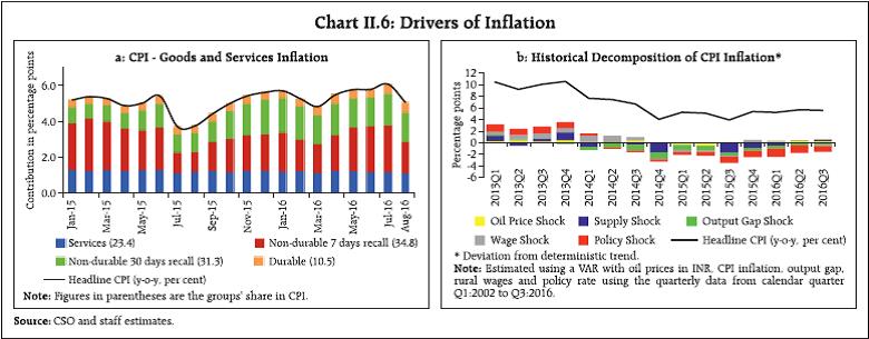 A historical decomposition of Inflation shocks also shows that in the April-July episode, it was the positive contribution of domestic supply shocks along with that of firmer international crude oil prices that resulted in the uptick in Inflation. Aggregate demand – embodied in the still negative output gap – along with continuing pass-through of past monetary policy tightening worked towards tempering Inflation pressures (Chart II.6b). In the food and beverages sub-group – the dominant category in the CPI with a weight of 46 per cent – Inflation rose steadily through April-July. The sharp, though delayed, correction in August was triggered by the compression in the contribution of vegetables. The food group contributed 59 per cent to average headline CPI Inflation during April-August, with price pressures mainly emanating from pulses, sugar and vegetables (Chart II.7). 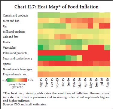 Pulses have been the major source of food Inflation consistently since Q2 of 2015-16 (Chart II.8). Reeling under two consecutive droughts, the production of pulses declined from 19.3 million tonnes in 2013-14 to 16.5 million tonnes in 2015-16 and the widening of the demand-supply imbalances elevated pulse prices unconscionably. As a consequence, pulses accounted for 22 per cent of food Inflation and 13 per cent of overall Inflation during April-August, despite a relatively low weight of 2.4 per cent in CPI. Excluding pulses, average food Inflation would have been lower by 1.2 percentage points and average headline Inflation by 0.6 percentage points during this period. In order to augment the supply of pulses, the Government undertook a number of measures, including higher imports at zero import duty, raising the buffer stock of pulses as well as minimum support prices (MSP). Although initially hamstrung by delayed arrival of imports, procurement at a time of high market prices and low offtake by States; the combined effects of these measures are increasingly visible in softening price pressures in pulses. Sugar emerged as the second major driver of food Inflation during first half of 2016-17 (Chart II.8). Despite adequate availability of stocks and reasonably good production, Inflation in this component rose sharply and remained in double digits from April, suggesting possible illicit stocking. Some moderation in sugar prices is expected by October 2016 as the cane-crushing season begins and fresh output is released in the market, although policy interventions may be warranted to ensure this outcome. A number of price control measures have been undertaken by the Government, including imposition of stock holding limits, extension of production subsidy, withdrawal of the mandatory export quota as well as extending financial assistance to the sugar mills through soft loan scheme. 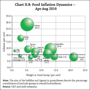 Food Inflation was also pushed up by a sharp uptick in prices of vegetables, especially tomatoes. Upside impulses started to manifest in April in a typical pre-monsoon sequence; however, pressures accentuated during June-July 2016 on account of the delayed onset of the south west monsoon. Food supply management strategies need to be informed by the spatial dynamics of Inflation. Empirical scrutiny of the stronger than anticipated firming of food price pressures during April to July 2016 in an analysis of variance (ANOVA) framework that tests inter alia for the equality of mean Inflation across states reveals significant spatial variations. Inter-state price differences turn out to be statistically significant for all sub-groups of food. Cereal prices show up pockets of high Inflation in Andhra Pradesh, Jharkhand and Odisha. Vegetables Inflation was highest in the eastern states of Odisha and West Bengal, and least in the hilly states of Himachal Pradesh and Jammu and Kashmir. Pulses Inflation, which averaged 30 per cent across the country, was relatively low at around 13 per cent in Assam and West Bengal (Annex Table II.1). These wide variations across states appear to be complemented by rising inter-state divergence in the case of commodities such as eggs, oils and fats, spices and sugar. This calls for integrating fragmented agricultural markets in the country, if food supply management policies have to be effective. Cluster analysis by sifting centre-level daily data from mandis3 points to strong regional variation in mark-ups from wholesale to retail prices for pulses, especially in the case of tur. In centres like Mumbai, Chennai, Delhi and Siliguri, the mark-ups for tur have been strikingly higher than in the rest of the country (Chart II.9). Thus, the sharp increase in retail prices in pulses, for example, is due to a combination of increases in wholesale prices and unduly large retail margins. 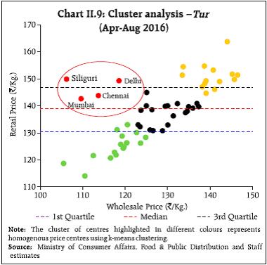 In the fuel and light sub-group, Inflation softened steadily through April-August. Electricity demand underwent a sustained moderation in an environment of subdued offtake from the manufacturing sector as well as from stress-laden distribution companies (DISCOMs). With the resulting compression in the demand supply gap, spot electricity prices fell below the average price in the power purchase agreement (PPA) contracts. LPG prices also declined sharply, largely influenced by the softening of international gas prices. International kerosene prices have hardened during the financial year so far, driving a wedge between the administered kerosene price which has been increased by ₹0.25 per litre per month beginning July 2016; under-recoveries on account of kerosene prices rose to ₹10.5 per litre effective October 1, 2016 from ₹6.5 per litre for March 2016. Inflation in respect of fuel items has diverged significantly between rural and urban areas with the latter, in fact, going into deflation in August. Items of fuel consumption in rural areas like firewood and dung cake reveal stickiness; on the other hand, fuel items in urban consumption are increasingly getting indexed to international prices (Chart II.10). CPI Inflation excluding food and fuel eased unevenly through April-August from 5.0 per cent in April to 4.6 per cent in August, with most of the sub-groups imbibing this halting moderation. Housing, clothing and footwear, and health were the main drivers (with a combined weight of 48 per cent in CPI excluding food and fuel), contributing 54 per cent of Inflation in this category (Chart II.11). Included in this sub-group under transportation, however, are petrol and diesel4; if they are excluded, Inflation excluding food and fuel (and petrol and diesel) would have moved down by less – from 5.3 per cent in April to 5.0 per cent in August (Chart II.12a). As alluded to in Chapter I, the implementation of the 7th CPC award starting August 2016 is expected to have a significant and drawn out impact on the CPI Inflation trajectory through both direct and indirect channels. These effects will be magnified as implementation spreads at the state level, as the experience with the 5th and 6th CPC awards have shown (Box II.1 of the April 2016 MPR provides a comprehensive assessment), playing out over a period of two years. These developments will have to be carefully monitored on account of the risks of getting generalised. Other Measures of Inflation Since outliers like vegetables and pulses impart a strong positive skew, trimming the Inflation distribution by removing specific portions of upper and lower tails of the distribution is widely used to understand underlying Inflation movements5, with the weighted median being a specific case of trimming. Trimmed means, the weighted median and exclusion-based measures of CPI Inflation reveal a central tendency at around 5 per cent during April-August 2016 (Chart II.12b). Inflation measured by other sectoral CPIs broadly tracked the movements in headline CPI. The wholesale price index (WPI), which had been in negative territory for 17 successive months, registered Inflation of 1.4 per cent in Q1 of 2016-17 that rose to 3.7 per cent in August 2016. As a result, the divergence between CPI and WPI Inflation, which was at 7.4 percentage points in 2015-16, narrowed down to 1.3 percentage points in August 2016. This reflected the bottoming out of the prolonged downturn in international commodity prices. Given the stickiness observed in services Inflation in the CPI, and the impending HRA effects of the 7th CPC award, it is unlikely that the divergence would reduce further. GDP and GVA deflators, which had been in the negative zone for two consecutive quarters, also started rising since Q4 of 2015-16 (Chart II.13). II.3 Costs Domestic farm and non-farm input costs embedded in the WPI have risen sequentially beginning October 2015, although the rates of increase are still benign (Chart II.14). In the farm sector, price rises in respect of high speed diesel, pesticides, tractors, fodder and cattle feed have contributed to the hardening of costs. Interventions such as ‘Make in India’ and the Government’s initiative to bring down prices of fertilisers by (a) reduction in non-urea prices for the first time in the last 15 years; and (b) increasing domestic production of fertilisers will have positive effects on the farm sector. 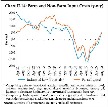 In the case of industrial inputs, sequential price increases in respect of mineral oil, metallic minerals and non-food articles – especially fibre and oil seeds – have started imposing cost pressures. The 75th round of the Reserve Bank’s industrial outlook survey (IOS) pertaining to July-September 2016 suggests that input price pressures are building up, with the rise in raw materials costs expected to continue into Q3. On the other hand, surveys of purchasing managers in manufacturing and services – that provide contemporaneous information – suggest that input and output price pressures still remain weak by histrocial standards. Rural wage growth exhibited divergent movements in its constituents. Rural non-agricultural wage growth has ebbed in recent months, possibly reflecting an increase in supply of non-agricultural labourers in rural areas due to weak construction activity attracting less labour migration to urban areas. In contrast, agricultural labour wage growth rose on the back of demand as sowing conditions improved. At the state level, agricultural wages increased, especially in foodgrain producing states such as Karnataka and Andhra Pradesh (Chart II.15). 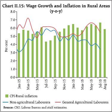 The proposed revision in basic minimum wages of the central sphere for different categories of employees (unskilled, semi-skilled, skilled, highly skilled and clerical)6 would support rural incomes that have been depressed by drought conditions for two successive years (2014-16). At the same time, however, it would push up headline CPI Inflation, as analysed in Chapter I. The expected increase in rural wages is also likely to bring on second round effects on Inflation. The Commission for Agricultural Costs and Prices (CACP) recommends MSP for agricultural commodities, including cereals and pulses, based inter alia on costs of production, labour and other inputs, with labour cost accounting for more than half of the total cost of production. While increases in MSPs for cereals have been moderate in the recent period – partly owing to the subdued growth in farm labour wages – the MSPs of pulses have been raised substantially on top of the sizable hike last year and are set to be raised even higher in the period ahead, with implications for the Inflation outlook. Wages in the organised sector reflected in staff costs per employee remained firm in Q1 of 2016-17 for both the manufacturing and the services sectors. On the other hand, unit labour cost measured by the ratio of staff cost to value of production, continued to rise for firms engaged in both sectors, notwithstanding some moderation in the case of manufacturing companies (Chart II.16). Looking ahead, Inflation developments are likelyto be shaped by the implementation of the GST.While the creation of a unified goods and servicesmarket in the country would reduce supply chainrigidities, cut down on transportation costs and alsobring down costs in general through improvementsin productivity, it could also produce a short-livedpass-through to the Inflation trajectory. The cross-countryexperience suggests that, controlling forcountry-specific characteristics, one-off effects tend todissipate after a year of its implementation (Box II.1). Box II.I: Inflation Impact of GST – Cross Country Evidence Internationally, 160 countries have some form of value added tax (World Bank, 2015). The experiences of the United Kingdom, Canada, New Zealand and Malaysia suggest that Inflation did increase in the period when GST was introduced (Table 1). Eventually, the Inflation impact moderated over a year, except in the case of United Kingdom where it remained elevated, due mainly to the oil crisis in 1973. Estimates of passthrough of changes in the VAT rate to consumer prices for 17 Euro zone countries for the period 1999-2013 show that, on average, the pass-through is much less than full and is highly sensitive to the type of VAT change. For changes in the standard rate, for instance, the final pass-through is about 100 per cent; for reduced rates, however, it is significantly less at around 30 per cent. The short-term effects on Inflation depend upon a host of factors, including the tax rate at which GST is implemented, the tax base and efficiency of the administrative machinery. | Table 1: Inflation Before and After GST Implementation (per cent) | | | t-1 | t | t+1 | t+2 | t+3 | t+4 | United Kingdom
[t =Q2:1973] | 7.9 | 9.3 | 9.2 | 10.3 | 12.9 | 15.9 | Canada
[t = Q1:1991] | 5.0 | 6.4 | 6.2 | 5.8 | 4.1 | 1.6 | New Zealand
[t = Q4:1986] | 10.7 | 18.7 | 18.6 | 18.9 | 16.6 | 8.6 | Australia
[t = Q3:2000] | 3.1 | 6.1 | 5.8 | 6.0 | 6.1 | 2.5 | Malaysia
[t = Q2: 2015] | 0.7 | 2.2 | 3.0 | 2.6 | 3.4 | 1.9 | | Source: OECD.Stat, Reserve Bank of Australia, Reserve Bank of New Zealand and Bank Negara Malaysia. | References: Benedek, Dora, Ruud De Mooij, Michael Keen and Philippe Wingender (2015), “Estimating VAT Pass-Through”, IMF Working Paper Series, WP/15/214, September. Government of India (2015), “Report on the Revenue Neutral Rate and Structure of Rates for the Goods and Services Tax”, Ministry of Finance, December 4. World Bank (2015), “Fiscal Policy for Equitable Growth,” India Development Report. The impact of the implementation of GST on CPI Inflation in India would largely depend on the standard rate that would be decided by the GST Council. The dual rate GST structure with a standard rate of 18 per cent and a low rate of 12 per cent (consistent with a revenue neutral rate (RNR) of about 15-15.5 per cent) is expected to have a minimal impact on Inflation (GoI, 2015)7. If the standard rate is increased to 22 per cent8 (consistent with an RNR of 17-18 per cent), the impact on aggregate Inflation would be in the range of 0.3-0.7 per cent, concentrated in select groups like healthcare (excluding medicines). As the standard rate increases from 22 per cent to 26 per cent and 30 per cent, the impact on CPI would increase from 0.6- 1.3 per cent and to 1.0-1.9 per cent (with input tax credit), respectively7. The general consensus is that the impact on consumer price Inflation is likely to be moderate if the standard GST rate is at 18 per cent – in fact, overall price levels may go down due to more efficient allocation of factors of production (NCAER, 2009)9. 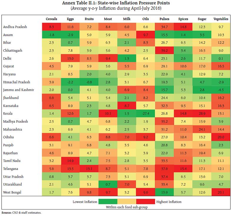
III. Demand and Output Aggregate demand slowed down in the first quarter of 2016-17, restrained by weak investment, but consumption spending is gradually improving. Aggregate supply conditions are poised to receive a strong boost from a reinvigoration of agriculture with some support from services, but industrial activity remains subdued. Economic activity lost some pace in the first half of 2016-17, relative to the preceding six months and a year ago. A deeper moderation has been cushioned by robust public spending. A retrenchment of investment has been underlying the slowdown; although public investment has been stepped up, crowding-in effects on private investment are not yet discernible. Private consumption spending has moderated somewhat, but a revival of agricultural activity and incomes and a sizable upward revision in wages and salaries in the public sector are set to boost it and regenerate growth impulses across the economy in the rest of 2016-17 and in the next year. While the weakness in domestic demand has sent imports into a prolonged contraction, the weakening global economy and financial market turbulence constitute the biggest risks to net exports and to overall economic activity, going forward. III.1. Aggregate Demand Measured by year-on-year (y-o-y) changes in real gross domestic product (GDP) at market prices, aggregate demand decelerated to a five-quarter low in Q1 of 2016-17, unable to sustain the strength of the upturn in the immediately preceding quarter (Table III.1). | Table III.1: Real GDP Growth (2011-12 Prices) | | (Per cent) | | Item | 2014-15 | 2015-16 | Weighted contribution 2015-16 * | 2014-15 | 2015-16 | 2016- 17 | | Q1 | Q2 | Q3 | Q4 | Q1 | Q2 | Q3 | Q4 | Q1 | | I. Private Final Consumption Expenditure | 6.2 | 7.4 | 4.1 | 8.2 | 9.2 | 1.5 | 6.6 | 6.9 | 6.3 | 8.2 | 8.3 | 6.7 | | II. Government Final Consumption Expenditure | 12.8 | 2.2 | 0.2 | 9.0 | 15.4 | 33.2 | -3.3 | -0.2 | 3.3 | 3.0 | 2.9 | 18.8 | | III. Gross Fixed Capital Formation | 4.9 | 3.9 | 1.3 | 8.3 | 2.2 | 3.7 | 5.4 | 7.1 | 9.7 | 1.2 | -1.9 | -3.1 | | IV. Net Exports | 11.7 | -36.6 | -0.5 | 62.8 | -72.5 | -111.0 | -6.6 | -47.6 | -41.3 | -29.0 | -11.0 | 93.5 | | (i) Exports | 1.7 | -5.2 | -1.2 | 11.6 | 1.1 | 2.0 | -6.3 | -5.7 | -4.3 | -8.9 | -1.9 | 3.2 | | (ii) Imports | 0.8 | -2.8 | -0.7 | -0.6 | 4.6 | 5.7 | -6.1 | -2.4 | -0.6 | -6.4 | -1.6 | -5.8 | | GDP at Market Prices | 7.2 | 7.6 | 7.6 | 7.5 | 8.3 | 6.6 | 6.7 | 7.5 | 7.6 | 7.2 | 7.9 | 7.1 | *: In percentage points. Component-wise contributions do not add up to GDP growth because change in stocks, valuables and discrepancies are not included here.
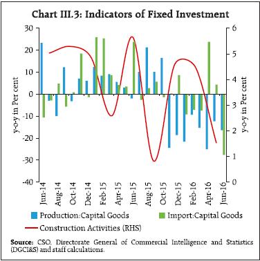
Source: Central Statistics Office (CSO). | The weakening of momentum was evident even on a seasonally adjusted basis (Chart III.1). In fact, aggregate demand was propped up by the front-loading of plan revenue expenditure; excluding the support from government final consumption expenditure, real GDP growth would have slumped to 5.7 per cent in Q1 of 2016-17, the lowest since Q4 of 2014-15 (Chart III.1). Demand conditions were undermined by a deepening of the contraction in gross fixed capital formation that set in from Q4 of 2015-16, besides a slowdown in private final consumption expenditure after two consecutive quarters of relatively robust growth. Weak domestic demand was also reflected in a sizable shrinking of imports, which enabled a positive contribution of net exports to aggregate demand after negative contributions for seven consecutive quarters. 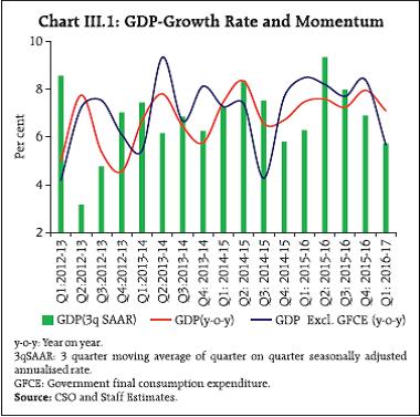 Investment demand has been muted through the first half of 2016-17, juxtaposing the absolute decline in gross fixed capital formation in Q1 of 2016-17 with more recent higher frequency indicators. Capex spending remains moribund even as industry is operating marginally below the long-term average of capacity utilisation on a seasonally adjusted basis (Chart III.2). Still significant financial stress in large brown field projects, especially in sectors such as iron and steel, construction, textiles and power continues to inhibit bank credit flows. Depressed construction activity and lacklustre demand for plant and machinery more generally is being mirrored in the coincident decline in production and imports of capital goods (Chart III.3). 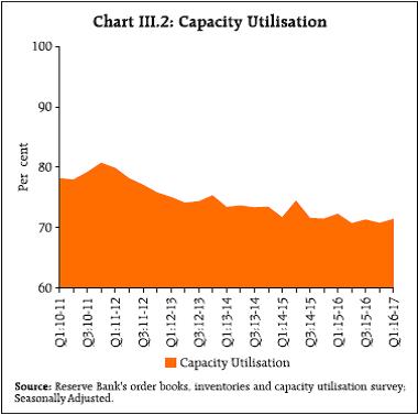
 reflecting the lacklustre investment climate, new investment intentions have slowed down by 19 per cent on y-o-y basis in Q2 of 2016-17 (Chart III.4). It needs to be noted, however, that the Project Monitoring Group is striving to galvanise new investments; it cleared 65 large projects in 2016-17 (up to September, 2016) worth ₹3.05 trillion (as compared with 89 projects worth ₹2.7 trillion in April- September, 2015-16). When these clearances fructify, these will increase the value of investment, with the majority of these projects in the roads, power, coal and petroleum sectors. While the stock of stalled projects declined by 44 per cent in Q1 and 28 per cent in Q2 of 2016-17 on a sequential basis – propelled by faster clearances, particularly in respect of non-environmental permissions – on-streaming of investment spending in these projects is yet to materialise, largely due to unfavourable market conditions. Meanwhile, sales of non-government non-financial companies have contracted, and both foreign direct investment and external commercial borrowings have slowed down in relation to their levels a year ago. 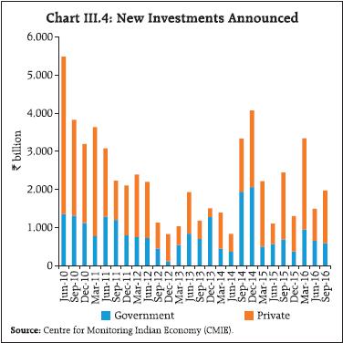 Even though private final consumption expenditure (PFCE) growth decelerated in Q1 in relation to immediately preceding quarters in tandem with the production of consumer goods, it continued to anchor the evolution of aggregate demand in the economy, contributing 52.3 per cent of real GDP growth. For the first half of the year cumulatively, a modest improvement in consumption spending may be taking root. Overall, consumer goods production slowed in July, but remained in positive territory for the third consecutive month on an improvement in the production of durables – reflective of the underlying resilience of urban consumption. Sales of passenger vehicles – another indicator of urban consumption demand – posted double-digit growth in July-August. Urban spending is poised to pick up with the implementation of the 7th CPC award on wages, salaries and pensions from August as well as from the ongoing preference of banks for relatively less risky retail and personal lending. Manufacturing purchasing managers index continued to point to modest expansion in employment since July 2016. Rural incomes and consumption spending should also receive a strong boost from the satisfactory spread and intensity of the south west monsoon, with the robust improvement in foodgrains production and acceleration in sales of tractors (excluding exports) and two-wheelers in August providing lead indications. While rural wage growth in April-July was slightly slower than a year ago, the implementation of the increase in minimum wages in the central sphere (see Chapter II) should improve rural incomes, going forward. Turning to government final consumption expenditure (GFCE) which provided strong support to aggregate demand in Q1, information gleaned from central government finances during Q2 so far (July-August, 2016) indicates this was sustained by a growth of 19.3 per cent in Plan revenue expenditure, largely in the form of spending on social and physical infrastructure1. Consequently, plan revenue expenditure in April- August rose as a proportion to budget estimates (BE) and on a year-on-year basis. Non-plan revenue expenditure was somewhat lower than a year ago in relation to BE for the first five months of 2016-17, with the expenditure on major subsidies and interest payments going through contractions in July-August 2016. Overall capital expenditure, however, increased in July-August, both on the plan and non-plan account, even as capital expenditure fell back marginally in relation to BE in April-August (Table III.2). | Table III.2: Key Fiscal Indicators – Central Government Finances (April-August) | | Indicator | Actual as per cent of BE | | 2015-16 | 2016-17 | | 1. Revenue Receipts | 30.3 | 28.0 | | a. Tax Revenue (Net) | 22.8 | 26.6 | | b. Non-Tax Revenue | 61.5 | 32.5 | | 2. Total Non-Debt Receipts | 29.7 | 27.3 | | 3. Non-Plan expenditure | 41.6 | 39.6 | | a. On Revenue Account | 42.0 | 39.9 | | b. On Capital Account | 37.0 | 35.3 | | 4. Plan expenditure | 40.1 | 43.0 | | a. On Revenue Account | 40.6 | 44.8 | | b. On Capital Account | 38.9 | 38.1 | | 5. Total Expenditure | 41.2 | 40.5 | | 6. Fiscal Deficit | 66.5 | 76.4 | | 7. Revenue Deficit | 74.7 | 91.8 | | 8. Primary Deficit | 206.9 | 565.9 | | Source: Controller General of Accounts (CGA), GoI. | Gross tax revenue recorded significant growth during April-August, led by buoyant income tax and excise duty collections (Chart III.5). The sharp growth in income tax collections in April-August reflected the change in advance tax payment requirements for individuals2, lower refunds by the Government than in the previous year and increase in surcharge3 on high net worth individuals. Within indirect taxes, while union excise duty collections were buoyed by higher consumption of petroleum products, the growth in the service tax receipts was significantly higher than a year ago due to the imposition of Krishi Kalyan cess at 0.5 per cent with effect from June 1, 2016. Non-tax revenue was, however, lower than last year as disinvestment failed to pick up despite conducive stock market conditions. In view of these developments, there was deterioration in the gross fiscal deficit (GFD) as a proportion to BE during April-August, mainly on account of a sharp increase in the revenue deficit. The Medium Term Expenditure Framework (MTEF) statement indicates that in order to absorb the complete impact of pay revisions in 2016-17, the provision for salary payments made in the Union Budget will require some enhancement in the revised estimates. The first batch of supplementary demands for grants for 2016-17 announced in August entails a net cash outgo of ₹209 billion over and above the BE. Therefore, fiscal spending may have to be restrained going forward in order to adhere to the target. The secondary impact of additional pay-out due to the Pay Commission recommendations on aggregate demand is likely to be muted as the revenue expenditure multiplier is found to be less than one in the Indian context4, partly reflecting the dampening impact of leakages through direct and indirect taxes. Moreover, as disbursements under the Pay Commission are undertaken without compromising the ongoing fiscal consolidation process, the growth enhancing impact will be moderate unlike the 5th and 6th Pay Commission awards. Taking into account the surge in Q1, net exports contributed to the increase in aggregate demand in the first quarter of 2016-17 through a large saving on account of cutbacks in major merchandise imports such as petroleum, oil and lubricants (POL), gold, iron and steel, and fertilisers. This was also reflected in the current account deficit narrowing to near-balance (0.1 per cent of GDP in Q1 from 1.2 per cent a year ago). Merchandise exports declined by 3 per cent in April- August in an environment of subdued global trade and output, and net terms of trade gains were eroded by the firming up of commodity prices. Emerging market economies (EMEs), which account for more than half of India’s export receipts, have suffered a persistent decline in their import volume (Chart III.6). 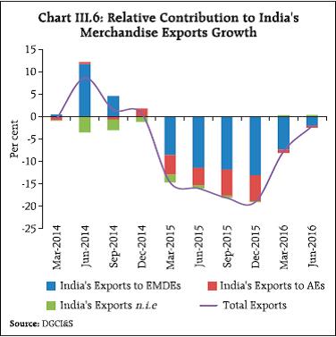 Gold import volume declined in April-August to almost a third of its level a year ago due to destocking of gold purchased earlier, subdued rural demand due to two consecutive poor monsoons and possibility of some supply through informal channels. The fall in non-oil non-gold imports in the year so far, particularly in the capital goods segment, reflects the weak domestic investment climate. Consequently, the merchandise trade deficit shrank sharply to US$ 34.7 billion in the first five months of 2016-17 from US$ 58.4 billion a year ago. Net services exports declined by over 10 per cent (April-July) as all major segments, except software services, were in contractionary mode. The prospects of private transfers, which had declined by about US$ 2 billion (a y-o-y decline of 11 per cent) in Q1, are uncertain as the prolonged softness in crude prices takes its toll on remittances from the Middle East. Disconcerting evidence has been forming for some time now that the engine of trade liberalisation that powered global output and trade since the 1980s in a rapidly integrating world marketplace is stalling. The ratio of world trade to GDP has been languishing since 2012, the longest phase of stagnation in the post-World War II period. The volume of world trade has plateaued since the beginning of 2015, even as underlying financial flows are coming off their pre-global crisis peaks. More recent evidence is pointing to a sharp drop in the demand for EME exports from AEs, particularly from the US, notwithstanding the recovery in US demand and the strength of the US dollar. While the biggest contraction of US demand is in respect of imports from China, imports from India have also fallen in value terms during 2016 so far. According to the International Monetary Fund (IMF), US imports from EMEs excluding China have been in contraction since 2015. This is being regarded as confirmation of the weakening of US manufacturing spreading to EMEs through the channel of trade5. Imports from EMEs by the European Union have also been contracting since 2015. Trade as a driver of world growth is on the wane, and instead a steady rise in protectionism is turning the tide of globalisation, possibly reversing it. India’s trade sector has also faced considerable protectionism in major partner economies. According to the Global Trade Alert database, Indian exports have been mainly impacted directly or indirectly through various types of measures, both tariff and non-tariff, in partner countries. III.2 Aggregate Supply Output measured by gross value added (GVA) at basic prices moderated marginally in Q1 of 2016-17 on a sequential y-o-y basis, although it was still a little above the average quarterly GVA growth recorded in 2015-16 (Table III.3). Seasonally adjusted q-o-q annualised growth indicates, however, a strengthening of momentum in Q1 relative to the immediately preceding quarter (Chart III.7a)6. | Table III.3: Sector-wise Growth in GVA | | (Per cent) | | Item | 2014-15 | 2015-16 | 2015-16 | 2014-15 | 2015-16 | 2016-17 | | Growth | Share | Q1 | Q2 | Q3 | Q4 | Q1 | Q2 | Q3 | Q4 | Q1 | | I. Agriculture, Forestry and Fishing | -0.2 | 1.2 | 15.4 | 2.3 | 2.8 | -2.4 | -1.7 | 2.6 | 2.0 | -1.0 | 2.3 | 1.8 | | II. Industry | 6.5 | 8.8 | 22.7 | 9.2 | 6.2 | 3.4 | 6.9 | 7.1 | 8.5 | 10.3 | 9.2 | 7.7 | | (i) Mining & quarrying | 10.8 | 7.4 | 3.1 | 16.5 | 7.0 | 9.1 | 10.1 | 8.5 | 5.0 | 7.1 | 8.6 | -0.4 | | (ii) Manufacturing | 5.5 | 9.3 | 17.5 | 7.9 | 5.8 | 1.7 | 6.6 | 7.3 | 9.2 | 11.5 | 9.3 | 9.1 | | (iii) Electricity, gas, water supply & other utilities | 8.0 | 6.6 | 2.2 | 10.2 | 8.8 | 8.8 | 4.4 | 4.0 | 7.5 | 5.6 | 9.3 | 9.4 | | III. Services | 9.4 | 8.2 | 61.9 | 8.0 | 9.9 | 11.7 | 8.3 | 8.3 | 7.9 | 8.5 | 8.1 | 8.4 | | (i) Construction | 4.4 | 3.9 | 8.5 | 5.0 | 5.3 | 4.9 | 2.6 | 5.6 | 0.8 | 4.6 | 4.5 | 1.5 | | (ii) Trade, hotel, transport, communication and services | 9.8 | 9.0 | 19.2 | 11.6 | 8.4 | 6.2 | 13.1 | 10.0 | 6.7 | 9.2 | 9.9 | 8.1 | | (iii) Financial, real estate & professional services | 10.6 | 10.3 | 21.6 | 8.5 | 12.7 | 12.1 | 9.0 | 9.3 | 11.9 | 10.5 | 9.1 | 9.4 | | (iv) Public administration, defence and other services | 10.7 | 6.6 | 12.6 | 4.2 | 10.3 | 25.3 | 4.1 | 5.9 | 6.9 | 7.2 | 6.4 | 12.3 | | IV. GVA at basic prices | 7.1 | 7.2 | 100.0 | 7.4 | 8.1 | 6.7 | 6.2 | 7.2 | 7.3 | 6.9 | 7.4 | 7.3 | | Source: CSO. |
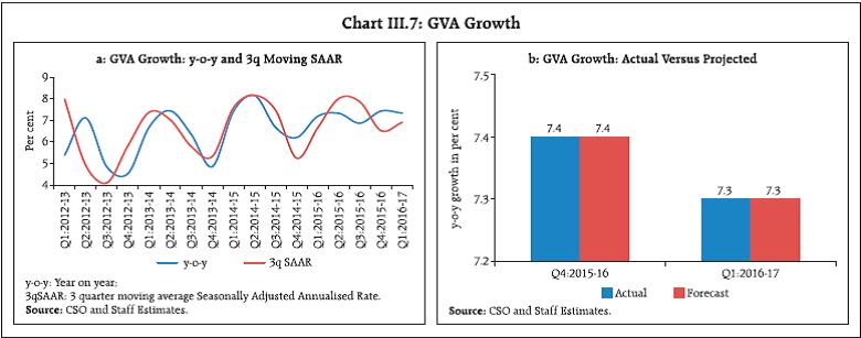 The April 2016 MPR had projected a gradual improvement in GVA growth from 7.3 per cent in Q1 to 7.7 per cent in Q2. With most of the initial assumptions underlying these projections materialising, the actual outcome for Q1 has matched the projection (Chart III.7b) (see Chapter I).Turning to Q2, the deceleration in value added in agriculture and allied activities in Q1 is well-positioned to reverse, although the upturn could undershoot the April 2016 projection slightly. The south-west monsoon commenced with a delay but soon gathered momentum and by mid-July, it had covered 89 per cent of the country’s meteorological sub-divisional area with excess/normal rainfall. From the second week of August, it waned in intensity and by end-September, precipitation was 3 per cent below the long period average (LPA) and was excess /normal across 85 per cent of the country’s meteorological sub-divisional area7. reflecting the initial delay in the monsoon’s onset, kharif sowing started on a low note, lagging behind last year’s acreage till first week of July. It picked up vigorously thereafter and by the end of September, it was 3.5 per cent higher than last year’s sown area, most notably under pulses (29.2 per cent), but also with respect to rice, coarse cereals and oilseeds. This has brightened the prospects of kharif crops production. According to the first advance estimates, the production of kharif foodgrains during 2016-17 at 135.0 million tonnes was 8.9 per cent higher than last year. The production of kharif pulses was a record high at 8.7 million tonnes. Among commercial crops, the production of oilseeds and cotton increased by 41.0 per cent and 6.6 per cent, respectively, over last year, even as that of sugarcane contracted. The satisfactory performance of the south west monsoon augurs well for the prospects of the rabi crops. The significant improvement in reservoir levels, especially in the Central and Western region, which accounts for around 64 per cent of irrigated area from these reservoirs, and the improvement in soil moisture conditions should enable the achievement of the rabi foodgrains target of 137.4 million tonnes (higher than that of 128.2 million tonnes last year). Growth of value added in the industrial sector in Q1 was pulled down by a contraction in mining and quarrying caused inter alia by a deceleration in the production of coal and absolute declines in the output of crude petroleum and natural gas. Turning to Q2, industrial production contracted in July, though a caveat is in order. Since the second half of 2015-16, movements in the index of industrial production (IIP) have been unduly influenced by a sharp contraction in the lumpy and large order-driven output of insulated rubber cables (IRC). It has produced strong and overwhelming effects on the headline index as well as on capital goods of which it is a component. Trimmed of IRC, industrial production would have risen by 3.2 per cent during April-July 2016 instead of contracting by 0.2 per cent. This is corroborated by the movements in a truncated IIP8 (Chart III.8). Manufacturing output contracted in July, although excluding IRC, it would have posted an expansion of 2.1 per cent. Nonetheless, manufacturing performance continues to face headwinds from the subdued business and investment environment. Illustratively, while sales of non-government manufacturing companies contracted in Q1 of 2016-17, profitability was shored up by other income and still soft input costs rather than a durable strengthening of output, with some indications of improvement in Q2. The corporate sector is challenged by high levels of leverage, relative to debt servicing capacity and concentration of risks. In this context, the vulnerability of the corporate sector to external debt has been amplified by low debt servicing capacity. 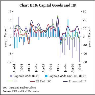 As regards other components of the IIP, electricity generation dipped in July after growing at a healthy pace in preceding months. It has fallen further in August due to contraction in thermal power generation – the first time in 16 months – with the plant load factor falling to a low of 52 per cent. Electricity demand has also been experiencing a sustained moderation in an environment of subdued offtake from the manufacturing sector as well as from stress-laden distribution companies (DISCOMs). The demand-supply gap narrowed to 0.5 per cent of total demand from 2.5 per cent a year ago. Consequently, suppliers sold electricity in the spot exchange – volumes reached a record high of 3,580 million units in July before dipping to 3,445 million units in August – bringing down exchange-traded spot prices to ₹2.20 per kilowatt hour (kWh), lower than prices under long-term power purchase agreements (PPAs). In terms of use-based activity, consumer nondurables slipped back into negative territory in July – a nine-month long slump had been interrupted by tentative positive growth in June – indicating that rural consumption is still weak. On the other hand, consumer durables have been supported by the abiding strength of urban consumption. While, basic goods decelerated, capital goods excluding IRC rose by barely 0.5 per cent in July, reflecting subdued investment demand. The recent momentum in core industries was sustained by a sharp pick-up in steel production in August 2016 reflecting inter alia low base and imposition of minimum import price, anti-dumping and safeguard duties. This, in consonance with the positive trend in cement production, augurs well for construction sector – even though the output of core industries as a whole was constrained by a decline in the production of coal, crude oil and natural gas, and deceleration in refinery products and electricity generation. The environment for industrial activity should improve with recent policy initiatives like liberalisation of foreign direct investment (FDI) policy in defence, civil aviation, pharmaceutical and broadcasting. This is being reflected in the manufacturing purchasing managers index which has remained in the expansionary zone since January 2016 mainly driven by new and export orders. Value added in the services sector, which constitutes around 63 per cent of total GVA, accelerated in Q1 on the back of stronger growth in public administration, defence and other services, supported by financial, real estate and professional services. On the other hand, activity in the construction sector slowed down and GVA growth in trade, hotels, transport and communication slowed sequentially. In Q2, public administration and defence services would have been boosted by the implementation of the 7th CPC award and one rank one pension (OROP) from August. The robust improvement in sales of two wheelers, passenger cars and tractors in recent months suggests that GVA in the transportation sub-sector is picking up (Table III.4). 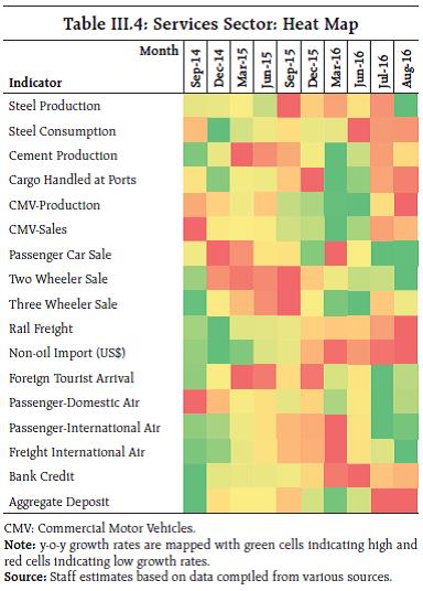 Construction activity remained subdued on account of stalled projects in the sector and onset of monsoon. As monsoon winds up, the construction sector is set for a turnaround on the package of measures approved by the Cabinet Committee on Economic Affairs (CCEA) to revive stalled projects, and especially the unclogging of cash flows. Available information shows that the construction of highways and capital expenditure under Railways are picking up and there are similar signs in respect of the sales of commercial properties in main cities. Though backed by low base, the consumption of steel accelerated in August after two months of contraction. Port cargo continues to decelerate, mostly on account of slowdown in imports of coal as domestic production picked up, and also due to contraction in tonnage of iron ore and fertilisers. Railway freight contracted due to low haulage of coal, and foodgrains, but it is expected to turn around once kharif procurement of foodgrains starts. Growth of foreign tourist arrivals accelerated on account of the e-visa facility. Accordingly, the services PMI improved further, driven by new business and improved business expectations in Q2. III.3 Output Gap The above assessments of the formation of aggregate demand and aggregate supply provide insights into the state of the economy vis-a-vis the underlying business cycle and, in turn, the trade-off between growth and Inflation confronting the setting of monetary policy. In this context, measurement of the potential level of output i.e., the sustainable level of output in which the intensity of resource use is non-Inflationary, becomes crucial. Bearing in mind that potential output is unobservable, that it has to be estimated and that these estimations are highly sensitive to the choice of period and methodology and the availability of data, staff has been employing the pragmatic approach. It combines a battery of methodologies, including different univariate filters - Hodrick–Prescott (HP); Baxter-King (BK); Christiano- Fitzgerald(CF); multivariate Kalman filter – with estimates of the production function approach in a principal components framework to derive a proximate view of potential output, while cautioning about the limitations with which these estimates have to be used (see MPRs of September 2015 and April 2016). The non-availability of a historical profile of GVA/GDP under the new series is also a major handicap to the accuracy of these estimates. Given these caveats, updated estimates of potential output suggest that the output gap – the deviation of actual output from its potential level and expressed as a percentage of potential output – remains negative, as it has been since 2015-16, but is slowly closing (Chart III.9). This is corroborated by the latest round of the Reserve Bank’s order books, inventory and capacity utilisation survey which shows capacity utilisation plateauing, after declining from 2011-12 (Chart III.2). 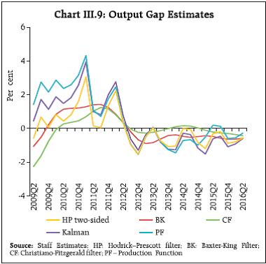 Economic activity is evolving in close alignment with staff’s projections, still below its underlying potential. Persisting slack in the economy has restrained a fuller expression of aggregate demand, which remains essentially consumption-driven. The continuing weakness in investment poses a risk not only to the prospects of the recovery gaining momentum on a durable basis but also to potential output itself. There is also some evidence, anecdotal and estimation-based, that productivity is getting impaired. Key to breaking out of this low-level trap is a revival of investment, especially private, in a conducive environment of reforms in product and factor supplies that unlock productivity and competitiveness, and raise the economy’s potential itself. This acquires urgency in view of the prolonged weakening of the global economy and the sense that global potential output may have become lastingly debilitated.
IV. Financial Markets and Liquidity Conditions Liquidity conditions have eased significantly, consistent with the accommodative stance of monetary policy. Bond yields touched multi-year lows. Commercial paper (CP) and corporate bond markets witnessed stronger transmission of monetary policy relative to the credit market, with issuances of CPs and corporate bonds increasing. Bank credit growth remains sluggish, albeit consistent with the nominal GDP growth outturn. Spells of turbulence have kept global financial markets unsettled since the April MPR, mainly sparked by worries about weakening global growth and diminishing confidence in the ability of central banks to nurture a sustainable recovery. In Q1 of 2016-17, equity, bond and commodity markets traded on a subdued note, with higher volatility and investor differentiation having widened credit spreads on EME and corporate assets. The universe of negative yields expanded rapidly in this risk-averse environment. The Brexit vote of June 23, however, took markets by surprise, causing equity, currencies and bonds to plunge across the globe. Yet, recovery too was surprisingly quick, especially in the context of a black swan type event. In Q2, volatility has subsided, commodity prices have firmed up, credit spreads have narrowed, equity markets have rallied to new highs and portfolio flows to EMEs have resumed. Although uncertainty around the Fed’s decision of September 21 did push up bond yields, other market segments maintained poise and risk appetite has intensified. Domestic financial markets have been resilient to these global developments and have, in fact, shown greater sensitivity to domestic cues. Even in the equity and foreign exchange segments, which are most vulnerable to global spillovers, the impact of international events has been transient. The Indian rupee turned out to be among the most stable currencies, notwithstanding fears about FCNR(B) redemptions commencing in September. In the money markets, interest rates have eased in the first half of 2016-17 propelled by comfortable liquidity conditions, and volatility has fallen. Bond yields touched multi-year lows, responding to abundant liquidity and expectations of falling Inflation cheered by a satisfactory monsoon. By contrast, credit markets have remained isolated in this generalised softening, with lending rate movements reportedly inhibited by asset quality concerns and balance sheet repair. Although deposit rates have also imbibed these rigidities, they have declined more than lending rates in recent months. IV.1 Financial Markets Q1 commenced with money markets fully transmitting the 25 bps cut in the repo rate of April 5. Liquidity conditions were influenced by restraint in government expenditure and a sustained elevation in currency demand entailing a leakage from the banking system during rabi procurement period of April and May. Open market purchases and term repos of varying tenors, in addition to the Reserve Bank’s normal liquidity operations, assuaged liquidity pressures. Consequently, the weighted average call money rate (WACR) and collateralised overnight rates traded tightly around the repo rate with a slight softening bias (Chart IV.1). The return of currency to the system towards the end of May and a pick-up in government expenditure in June helped to ease liquidity conditions. 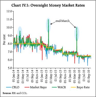 Two developments are noteworthy in the evolution of money market in this period. First, with the relaxation in reserve maintenance norms (to a daily minimum of 90 per cent from 95 per cent earlier) as part of the refinements in the liquidity management framework in April (see section IV.2), there was a moderation in banks’ holdings of excess reserves (Chart IV.2). Secondly, the market response to the narrowing of the policy rate corridor to +/-50 bps on April 5 was reflected in a compression of money market spreads vis-à-vis the repo rate and a decline in volatility (Chart IV.3). 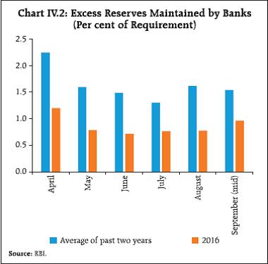
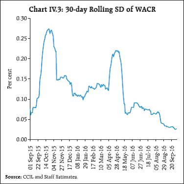 With the evolution of liquidity condi tions passing a tipping point in June, a new phase was evident in Q2, aided by the return of currency to the banking system, stepped up government expenditure – necessitating ways and means advances (WMA) from the Reserve Bank – and stronger mobilisation of deposits. Accordingly, the Reserve Bank switched into a liquidity absorption mode with variable rate reverse repo operations, including of 28-day tenor for the first time. Surplus transfer from the Reserve Bank was quickly followed by large coupon payments and redemptions in mid-August. The WACR remained below the repo rate throughout, tracked by other overnight money market rates. In fact, on 95 per cent of the trading days in the first half of 2016-17 (excluding Saturdays), the WACR traded marginally below the repo rate (by about 11 bps on an average). The benign effects of comfortable liquidity conditions in the overnight segments spread through the continuum of money market rates, easing term premia and softening three-month CP and certificate of deposit (CD) rates to intra-year lows. In fact, CP rates fell well below the weighted average lending rate (WALR) on fresh rupee loans of up to one-year maturity, rendering CP issuances an attractive alternative for raising working capital funds in an environment characterised by risk aversion among banks (Chart IV.4). Higher rated corporates raised ₹1.37 trillion in the first half of the year (up to mid- September 2016) through CPs. 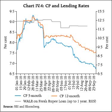 The implementation of the Basel III liquidity coverage ratio (LCR) has impacted liquidity in money markets across the world. In order to cushion these pressures, the Reserve Bank has been providing banks headroom by allowing carve-outs in the prescription of SLR cumulating to 11 per cent of NDTL, including 2 per cent available under the marginal standing facility (MSF). In this sense, the SLR has enabled a frictionfree transition to the LCR relative to the cross-country experience (Box IV.1). Box IV.1: Basel III Liquidity Coverage Ratio and the Operating Target of Monetary Policy The phased introduction of the Basel III Liquidity Coverage Ratio (LCR) since January 2015 across jurisdictions has altered volume and rates in the unsecured segment of the money market, posing challenges for the implementation of monetary policy (Bonner and Eijffinger, 2012; and Schmitz, 2013). Under the LCR regulation, a bank’s stock of high quality liquid assets (HQLA) must exceed its projected total net cash outflows over the next 30 calendar days under a stress scenario. Any borrowing from the uncollateralised market of less than 30 days maturity attracts a run off rate of 100 per cent, i.e., to be repaid within 30 days, and therefore, would require 100 per cent HQLA backing. A bank can borrow and retain cash as part of HQLA to avoid a fall in LCR, but in that case borrowed liquidity cannot be used for non-HQLA asset financing. This is observed to have altered banks’ activity in the call money market in the post-LCR regime. Generalised method of moments (GMM) estimates in a dynamic panel data regression framework involving monthly data on bank-wise LCR positions relative to the prescribed norm, capital to risk weighted asset ratios (CRAR), gross non-performing assets (GNPA) as a ratio of total assets and a dummy* to capture the impact of the LCR on the money market show that banks operating closer to the prescribed LCR norm tend to borrow at a higher rate in the call market (Table 1). Banks with higher CRAR seem to have the advantage of borrowing at a lower rate, while banks with higher GNPA have to pay higher rates on their call borrowings. While the WACR (and call volumes) are sensitive to the LCR regulation, the overall impact on the WACR is limited to 7 bps. Thus, the accommodation provided to banks within the prescribed SLR has been critical in mitigating adverse effects of the LCR on the WACR. | Table 1: Estimated Impact of LCR on Call Market Spread and Volumes | | WACR Spread over Repo Rate | Call Market Borrowing to Total Asset Ratio | | Dep. Var. | Dynamic GMM | Dep. Var. | Dynamic GMM | | Coeff. | P-val | Coeff. | P-val | | Constant | -0.090 | 0.18 | Constant | 12.180 | 0.05 | | Spread(-1) | -0.200 | 0.00 | CallVol(-1) | 0.180 | 0.00 | | LCRD(-1) | 0.070 | 0.02 | CallVol(-2) | -0.400 | 0.00 | | CRAR (-3) | -0.004 | 0.00 | LCRD(-1) | 6.150 | 0.08 | | GNPA (-3) | 0.060 | 0.01 | CDratio | 0.0004 | 0.00 | | | Wald Chi-square | 33.03 (0.00) | | Wald Chi-square | 167.1 (0.00) | | | AR(1) | -5.51 (0.00) | | AR(1) | -2.29 (0.02) | | | AR(2) | -1.66 (0.10) | | AR(2) | -0.35 (0.72) | | | Sargan stat. (2-step) | 58.89 | | Sargan stat. (2-step) | 61.1 | | * The dummy assigns a value of one to banks with LCR positions within 10 per cent above the prescribed norm and zero otherwise; given that the prescribed LCR in India was raised to 70 per cent in January 2016, banks operating at less than 80 per cent LCR could be expected to borrow in the call market at a higher rate relative to others. | References: Bonner, Clemens and Sylvester Eijffinger (2012), “The Impact of the LCR on the Interbank Money Market?”, De Nederlandsche Bank Working Paper No.364, December. Schmitz, Stefan W (2013), “The Impact of the Liquidity Coverage Ratio (LCR) on the Implementation of Monetary Policy”, Economic Notes, Wiley Blackwell, June. Bond markets began Q1 on a firm note as investors engaged in consolidation and profit-booking, although by early May, a softening bias set in as fears of a hike in the US federal funds rate receded and the Reserve Bank’s open market operations lifted sentiment. As Inflation moved up higher than expected, however, gilt yields hardened and rising international crude prices added an upside. Foreign portfolio investors (FPIs) sold net debt amounting to ₹106 billion during May and June. Bond markets were least impacted by Brexit, with 10-year FIMMDA generic yields moving up by eight basis points only on June 23, and softening immediately thereafter. With Inflation in India rising beyond the usual seasonal upturn at this time of the year, yields remained range-bound in June, although open market purchase operations continued to provide comfort. Starting in mid-June, gilt yields softened into Q2 with abundant liquidity and optimism generated by the satisfactory progress of the monsoon lifting sentiment, notwithstanding the peaking of Inflation in July which the market had fully priced in. The post-Brexit resumption of portfolio flows into the gilt segment of the bond markets also softened yields. Trading volumes in the secondary market increased from a daily average of ₹489 billion in June to ₹1057 billion in July and ₹935 billion in August. A substantial part of the increase in activity was on account of global funds, pushed out of advanced economies by negative yields, and also profit booking by banks. The new 10-year benchmark announced on August 29, 2016 had a dramatic effect. In the ‘when issued’ market, it closed at 6.98 per cent on September 2, when trading ceased in that segment, setting the stage for the OTC market. The 10-year benchmark yield touched a multi-year low of 6.80 per cent in the secondary market on September 23. In H1 of 2016-17, gilt yields have eased by more than 50 bps as against a policy repo rate cut of 25 bps (Chart IV.5). Market sentiment was also buoyed by the announcement of a number of measures by the Reserve Bank and SEBI to improve depth and liquidity in the market1. 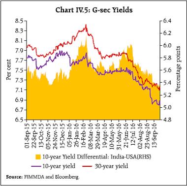 In the corporate bond segment, issuances fell by 4.1 per cent in Q1 indicating subdued corporate investment with a preference for refinancing rather than investing in new capacities. Corporate bond yields – especially on AAA corporate bonds – declined significantly in Q2, tracking gilts. This galvanised a spate of issuances to take advantage of the rate differential vis-à-vis bank lending rates. Overall resources mobilised through private placement increased by around 12 per cent in H1 (up to August) over the corresponding period of last year. While FPI investment in corporate bonds witnessed net outflows till August 2016 mainly due to narrowing of interest rate differentials and stable hedging costs, investment by mutual funds (excluding PSU bonds) increased by around 31 per cent over March 2016. Corporates also raised resources through issuances of masala bonds. These bonds are denominated in rupees and entail no exchange rate risk for the issuers. In the financial year so far, companies have raised around ₹88 billion through masala bonds. With these alternative avenues, corporates have cut down substantially on their recourse to external commercial borrowings. Equity markets experienced choppy trading in Q1. The Brexit referendum triggered some panic FPI selling, but in the last week of the month, the Sensex recovered these losses and posted increases on the back of optimism over the progress of the monsoon and the Cabinet’s approval of the 7th Pay Commission recommendations. Equity markets turned up in Q2, supported by rejuvenation of FPI buying interest and recovery in global equity markets over expectations of expanded accommodation in monetary policies of systemic central banks. The prospects of the GST coming into force also lifted market sentiment. Overall, the benchmark BSE Sensex posted a gain of around 21 per cent over its February 2016 level in the first half of 2016-17. Mid-cap and small-cap stocks outperformed the benchmark indices, pointing to a greater significance of domestic macroeconomic conditions relative to the global economy for these firms. These developments have focused interest in market valuations. The price-to-earnings (PE) ratio of the Sensex was at 20.7 at end-September as against a range between 7.3 (Russia) and 25.7 (South Africa) for other EMEs. Through the first half of 2016-17, resource mobilisation through IPOs and right issues has been high – 32 companies raised ₹162.9 billion in H1 as against ₹126.6 billion during the same period a year ago. What is interesting is that this recent buoyancy in IPOs also evinced strong retail interest – the average number of times the retail portion of the IPO subscription rose from about 2.4 in 2015-16 to 7.7 in 2016-17 so far. The gains made on listing mirrored this surge in retail participation – the average listing premium rose from 5.1 per cent in 2015-16 to 22.5 per cent in 2016-17. In the foreign exchange market, the rupee traded with a depreciating bias against the US dollar in Q1, mainly reflecting the strengthening of the US dollar against EME and commodity currencies and the yen on the back of weak macroeconomic data out of China and renewed political turmoil in Brazil. Higher than expected Inflation readings and import payment-related foreign currency buying by oil marketing companies and PSUs also impacted the rupee’s movements. FPI outflows, particularly from the debt segment, kept the rupee under downward pressure, which intensified with the Brexit vote; however, the rupee recovered ground swiftly, as sentiment improved and FPI flows returned vigorously. Viewed in relation to EME peers, rupee moved in a narrow band, even as several other currencies appreciated in nominal terms, some of them going through corrections of sizable past depreciation. The bounce back from Brexit sustained an appreciating bias in the rupee’s movements into Q2, with intermittent downsides from the strength of the US dollar. Nonetheless, an overall optimism in the rupee was evident in the strong resumption of FPI inflows in both the equity and debt markets. While the rupee traded range-bound in the rest of Q2, uncertainty reflected in one-month implied volatility increased. The rupee moved in a narrow range against the US dollar and the euro in H1. It appreciated strongly against the pound sterling, but depreciated against the Japanese yen, mirroring cross-currency movements against the US dollar (Chart IV.6). In terms of the nominal effective exchange rate index (36-currency basket), the rupee exhibited stability through H1, whereas in terms of the real effective exchange rate index, it appreciated by 3.6 per cent since March 2016 (Table IV.1). | Table IV.1: Nominal and Real Effective Exchange Rates: Trade-Based (Base: 2004-05=100) | | Item | Index: September 23, 2016 (P) | Appreciation (+) / Depreciation (-) (per cent) | | September 23 over March 2016 | March 2016 over March 2015 | | 36-currency REER | 114.59 | 3.6 | -2.3 | | 36-currency NEER | 74.50 | 1.1 | -4.1 | | 6-currency REER | 126.42 | 3.7 | -3.1 | | 6-currency NEER | 66.97 | 0.7 | -6.6 | | ₹/ US$ (As on September 30, 2016) | 66.66 | 0.5 | -6.8 | P: Provisional.
Note: REER figures are based on Consumer Price Index (Combined). | In the credit market, activity weakened as non-food credit growth remained sluggish through H1 (Chart IV.7). Movements in credit flows, however, need to be juxtaposed against two developments which suggest that underlying credit market activity may not have been as feeble as the headline numbers suggest. First, banks have written-off/sold loans to asset reconstruction companies (ARCs), which effectively compressed their loan books. Second and more importantly, more than half of the Ujawal DISCOM Assurance Yojana (UDAY) bond issuances during the financial year so far represent conversion/swapping of bank credit into special securities. Adjusting for the UDAY bond issuances, the flow of non-food credit to the economy during H1 (up to September 16, 2016) was comparable to that in the corresponding period of last year (Chart IV.8). In terms of industry sub-sectors, bank credit to chemicals, textiles, food processing and mining further contracted. Non-banking sources of funding for the commercial sector, both foreign and domestic, also remained subdued. As a result, the total flow of resources to the commercial sector during the year (up to September 16, 2016) was lower by about 15 per cent than a year ago. 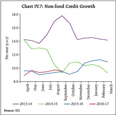
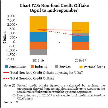 The Reserve Bank instituted a new lending rate system for banks – the marginal cost of funds based lending rate (MCLR) system – effective April 1, 2016 (Box IV.2). During H1 of 2016-17, the median one-year MCLR of PSBs and private sector banks declined by 15 bps and 25 bps, respectively (Chart IV.9). Banks have, however, increased the spread and term premia over the same period, effectively leaving the WALR on outstanding rupee loans unchanged. For fresh rupee loans, the WALR declined by 5 bps (April-August). Rupee loans that are being disbursed since April 1, 2016 are priced at the MCLR, and therefore, the base rate continues to account for a substantial share in the pricing of outstanding credit. 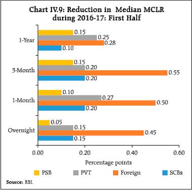 A comparison of the behaviour of key components of the MCLR reveals that the marginal cost of funds has moderated in respect of both PSBs and private sector banks, driven down by the marginal cost of borrowings (Chart IV.10). On the flip side, the expected return on net worth has increased from an already elevated level. Box IV.2: Transmission under the BPLR, Base Rate and MCLR Regimes The benchmark prime lending rate (BPLR) system introduced in 2003 fell short of its original intent of serving as the reference rate for pricing loan products linked to the actual cost of funds. Perversely, the share of sub-BPLR lending rose as high as 77 per cent by September 2008, concentrated at longer term tenors (above three years), effectively undermining the BPLR. Residential housing and consumer durables were outside the purview of the BPLR and sub-BPLR lending became a source of distortion in terms of cross-subsidization across borrower categories. The base rate system, which came into effect in July 2010, was meant to guard against the arbitrary pricing of loans prevalent under the BPLR system by disallowing loans at sub-prime rates. However, discrimination in the pricing of credit between new and old customers continued as banks often tweaked the spread over the base rate. The flexibility accorded to banks in the determination of cost of funds – average, marginal or blended cost – rendered assessment of transmission difficult. The MCLR system introduced on April 1, 2016 was designed taking into account limitations of both the BPLR and the base rate regimes. Under the MCLR system, banks determine their benchmark lending rates linked to marginal cost of funds. The MCLR consists of four components: (a) marginal cost of funds (i.e., marginal cost of borrowings comprising deposits and other borrowings, and return on net worth), (b) negative carry on account of cash reserve ratio (CRR), (c) operating costs and (d) term premium/discount for prescribed maturities. The MCLR plus spread is the actual lending rate for a borrower. The spread comprises two components, viz., business strategy and credit risk premium. In principle, the role of each component of the MCLR can be monitored and analysed. Different components of the MCLR vary widely across banks at any point in time, reflecting: (i) differences in the composition and maturity profile of their liabilities – current, savings and time deposits - and the extent of reliance on retail vis-a-vis wholesale customers, which has a bearing on the cost of funds; (ii) divergences in the operating cost environment of banks arising from differences in the use of technology, quality of human capital and the geographical spread of bank branches; and (iii) the return on net worth expected by banks. An inter-temporal comparison of monetary policy transmission shows that the magnitude of transmission varies across regimes and policy cycles. The transmission of monetary policy is marked by long and variable time lags with asymmetric market responses to policy impulses – generally higher during a tightening phase and lower during an easing phase, irrespective of the prevailing regime for pricing of credit (Table 1). In the current environment, factors that continue to impede transmission include: (i) fixed interest rates offered on savings deposits (though deregulated) which, along with current accounts, constitute around 35 per cent of aggregate deposits, thereby stifling transmission to more than a third of deposits; (ii) no reduction in interest rates on small savings in Q2 of 2016-17, followed by a marginal reduction of 10 bps in Q3, notwithstanding a notable decline in G-sec yields; (iii) stressed asset quality of banks and pricing of risk premium reflecting risk aversion; and (iv) sluggish demand for bank credit. | Table 1: Transmission Under Different Regimes and Policy Cycles (Change in median rate in basis points) | | Phase | Policy Variables | Public Sector Banks | Private Sector Banks | Foreign Banks | | CRR | Repo Rate | Reverse Repo Rate | BPLR | Base Rate | MCLR
(1 Year) | BPLR | Base Rate | MCLR
(1 Year) | BPLR | Base Rate | MCLR
(1 Year) | | Tightening | | | | | | | | | | | | | | Apr 2004- Sep 2008 | 450 | 300 | 150 | 300 | | | 337 | | | 132 | | | | Easing | | | | | | | | | | | | | | Oct 2008- Feb 2010 | -400 | -425 | -275 | -200 | | | -37 | | | 13 | | | | Tightening | | | | | | | | | | | | | | Mar 2010-June 2010 | 100 | 50 | 50 | 0 | | | 0 | | | 0 | | | | Jul 2010- Mar 2012 | -50 | 325 | 375 | 300 | 275 | | 262 | 283 | | 12 | 250 | | | Easing | | | | | | | | | | | | | | Apr 2012-June 2013 | -150 | -125 | -125 | -25 | -50 | | 0 | -8 | | 25 | -30 | | | Tightening | | | | | | | | | | | | | | July 2013-Dec 2014 | 0 | 75 | 75 | 0 | 0 | | 33 | 25 | | 0 | 30 | | | Easing | | | | | | | | | | | | | | Jan 2015-Mar 2016 | 0 | -125 | -125 | 0 | -55 | | -8 | -50 | | 0 | -62 | | | Apr 2016- Sep 2016 | 0 | -25 | 25 | -7 | -5 | -15 | -125 | 0 | -25 | 0 | -13 | -28 | IV.2 Liquidity Conditions and the Operating Procedure of Monetary Policy Under the amended RBI Act, 1934 and related notifications, the Reserve Bank is enjoined to set out the operating procedure of monetary policy and any changes thereto in the public domain. This operating procedure – embodied in the Reserve Bank’s liquidity management framework – was published in the April 2015 MPR, Box IV.I. The central premise of the operating procedure is to achieve the operating target of monetary policy – to align the weighted average call money rate (WACR) with the repo rate through active liquidity management, consistent with the stance of monetary policy. Based on continuous assessment of the performance of the operating framework in pursuit of this objective and the evolving nature of liquidity demand in the economy, major changes were introduced in the framework in April 2016, which included: (a) narrowing the liquidiy adjustment facility (LAF) corridor around the policy repo rate from +/- 100 bps to +/-50 bps; (b) smoothening the supply of liquidity through timely use of open market purchase/ sale auctions in conjunction with normal liquidity facilities and fine-tuning operations; (c) progressively lowering the ex ante liquidity deficit in the system to a position closer to neutrality; and (d) reducing the minimum daily maintenance of the CRR from 95 per cent of the requirement to 90 per cent. Since the introduction of these refinements in the liquidity management framework, the Reserve Bank has injected liquidity of ₹1.01 trillion through open market operations (OMOs) in the first half of the year. Including the liquidity impact of foreign exchange market operations, the net injection of permanent liquidity was of the order of about ₹1.6 trillion (Chart IV.11), which has significantly offset the influence of the two key autonomous drivers of liquidity – cash balances of the Government and currency demand (Chart IV.12). 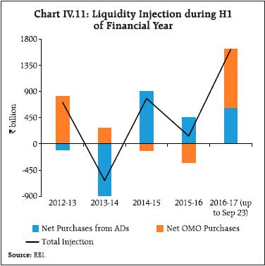
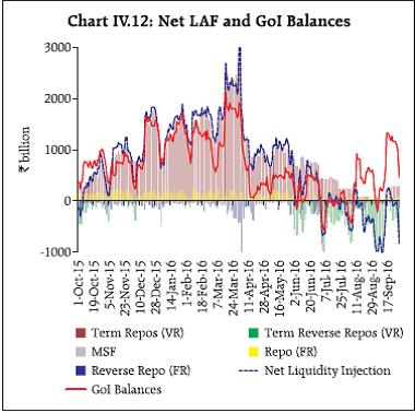 In Q1, currency demand increased by ₹600 billion in the first three weeks of April. Accordingly, ₹300 billion was injected through open market purchases in April and ₹400 billion in May to accommodate the higher liquidity deficit in the system, given the access to the LAF averaging around ₹1 trillion. Gyrations in liquidity conditions were influenced by fluctuations in Government cash balances and other frictional factors which were evened out through fine-tuning operations involving variable rate repo auctions of tenors ranging between 5 days and 21 days. In Q2, with the Government taking recourse to WMA and overdrafts (ODs) in the first week of July, the liquidity conditions moved to a surplus. Fine-tuning term reverse repo auctions – the key instrument for absorbing surpluses – exceeded ₹1 trillion around this time. Easy liquidity conditions persisted in early August, reaching near balance when the Reserve Bank transferred its surplus to the Government on August 11. With government spending picking up, subdued currency demand during July and August, and proactive front-loading of liquidity by the Reserve Bank in anticipation of potential pressure associated with redemptions of FCNR(B) deposits kept liquidity conditions in surplus mode. In the early part of September, with the Government resorting to WMA again, the net LAF absorption reached ₹1 trillion. In anticipation of liquidity pressures arising from advance tax payments in September, the Reserve Bank conducted an OMO purchase auction of ₹100 billion on September 8. Liquidity deficit returned to a surplus mode by the end of the month. Structural and cyclical factors impeding transmission to bank lending rates, particularly stressed balance sheets of banks and sluggish credit growth, may require a review of the MCLR implementation by banks, given the context of significant softening of long-term yields. In this scenario, the Reserve Bank would continue to manage liquidity proactively and consistent with the stance of monetary policy, while taking timely and appropriate measures to insulate the system from shocks.
V. External Environment Global economic activity and trade remain subdued in 2016 so far. While advanced economies (AEs) confront persisting slack and low inflation, several key emerging market economies (EMEs) have had to contend with slower economic activity and sluggish investment. Since the MPR of April 2016, global growth and trade have weakened and new risks to the outlook have slanted the balance further to the downside. Industrial activity, in particular, has slumped, going into contraction in some AEs. Rising protectionism is threatening to accentuate the compression of trade volumes. While commodity prices have firmed up, the outlook remains subdued. Crude oil prices rose to a recent peak in Q2 of 2016 but mostly on supply disruptions across geographies. In Q3, this upturn has been curbed by higher inventories. Prices of precious metals have been buoyed by safe haven demand, a telling insight into the state of the global economy. Food prices remain elevated on harvest failures in several parts of the world. Inflation remains subdued in AEs and has started to edge down in EMEs. International financial markets were shocked by the outcome of Brexit referendum in Q2, with equity markets plunging worldwide, currency volatility heightening and investors herding into safe havens. Markets quickly stabilised, and moved up in Q3. However, incoming data can dispel this uneasy calm, as the uptick in bond yields – out of a widening negative universe – in the run-up to the Fed’s September meeting has shown. Equity prices regained lost ground and currencies recovered, but uncertainty surrounding the monetary policy stances of systemic central banks will likely continue to impart volatility to currency and equity markets. Capital flows are returning to EMEs, though foreign direct investment has not sustained the pace it achieved a year ago. V.1 Global Economic Conditions The US economy slowed in the first half of 2016, despite the higher than expected upturn in Q2. The impetus from private consumption, non-residential fixed investment and exports was offset by drops in inventory accumulation, residential fixed investment and government spending. Investment in Q2 declined for three consecutive quarters as companies cut back spending on oil wells, equipment and inventories. In Q3, factory activity contracted for the first time in six months in August amidst slumping orders and production. Labor market conditions, on the other hand, rebounded to positive territory in July from a six-month slump and continued to improve in the rest of Q3 with low levels of layoffs in August and a drop in jobless claims to a two-month low in September. In the Euro area, growth decelerated from Q1 to Q2, both sequentially and y-o-y. Net exports and consumer spending supported growth, but fixed investment and inventories operated as drags. Industrial production contracted in July. The re-emergence of stress in some parts of the banking sector in Q3 tightened financial conditions. However, economic sentiment improved in September in its major economies. The Japanese economy decelerated in Q2 after a modest improvement in Q1, as weak domestic consumption and sluggish external demand prompted companies to cut capital spending. In the UK, economic growth was stronger in Q2 than Q1, even as industrial growth was partly offset by a fall in construction activity. The outlook for Q3 is subdued with the fuller effects of Brexit yet to play out (Table V.1). | Table V.1: Real GDP Growth (q-o-q, annualised) | | (Per cent) | | | 2015: Q2 | 2015: Q3 | 2015: Q4 | 2016: Q1 | 2016: Q2 | 2016 (P) | 2017 (P) | | Advanced Economies (AEs) | | | | | | | | | US | 2.6 | 2.0 | 0.9 | 0.8 | 1.4 | 2.2 | 2.5 | | Euro Area | 1.6 | 1.2 | 1.6 | 2.4 | 1.2 | 1.6 | 1.4 | | Japan | -1.9 | 2.1 | -1.7 | 2.1 | 0.7 | 0.3 | 0.1 | | UK | 2.0 | 1.2 | 2.8 | 1.6 | 2.8 | 1.7 | 1.3 | | Canada | -0.5 | 2.2 | 0.5 | 2.5 | -1.6 | 1.4 | 2.1 | | Emerging Market Economies (EMEs) | | | | | | | | | China | 7.2 | 7.2 | 6.0 | 4.8 | 7.2 | 6.6 | 6.2 | | Brazil | -9.1 | -6.2 | -5.1 | -1.7 | -2.2 | -3.3 | 0.5 | | Russia* | -4.5 | -3.7 | -3.8 | -1.2 | -0.6 | -1.2 | 1.0 | | South Africa | -2.0 | 0.3 | 0.4 | -1.2 | 3.3 | 0.1 | 1.0 | | Korea | 1.6 | 4.8 | 2.8 | 2.0 | 3.2 | 2.7 | 2.9 | | Thailand | 2.1 | 3.6 | 3.4 | 4.0 | 3.2 | 3.0 | 3.2 | | Malaysia | 3.6 | 3.6 | 4.8 | 4.0 | 2.8 | 4.4 | 4.8 | | Mexico | 3.3 | 2.8 | 1.8 | 2.0 | -0.7 | 2.5 | 2.6 | | Saudi Arabia** | -4.7 | 2.1 | 5.9 | 2.8 | - | 1.2 | 2.0 | | Memo | | | | | 2015 | 2016 (P) | 2017 (P) | | World Output | | | | | 3.1 | 3.1 | 3.4 | | World Trade Volume | | | | | 2.7 | 1.7 | 1.8 - 3.1 | P : Projection, * year-on-year, **: Seasonally Unadjusted.
Source: Bloomberg, IMF, WTO and Eurostat. | Among major EMEs, growth performance in recent quarters remains divergent. The recent uptick in commodity prices has provided some relief to commodity exporters, while net terms of trade gains for commodity importers are moderating. In China, growth held steady at 6.7 per cent y-o-y in Q2 on the back of strong policy stimulus. Private investment growth, however, shrank to a record low. In Q3, factory output and retail sales grew faster than expected in August, underpinned by housing market and government infrastructure spending. By contrast, the Brazilian economy continues to face deep recession in the midst of political uncertainty undermining consumer and business confidence, but the recent uptick in commodity prices could alleviate some stress. In Russia, recessionary conditions are diminishing as reflected in the economy contracting at a slower rate in Q2 on the support of a modest pick-up in the industrial sector and transportation services. The South African economy continued to weaken in Q2, following a contraction in Q1, due to slowing demand from China and low commodity prices. China and India are projected to contribute more than half of global growth in 2016 (Chart V.1). The OECD’s composite leading indicators point to stable growth in the US, the Euro area and Japan, and a pick up in growth momentum in China, Russia, Brazil and India (Chart V.2). 
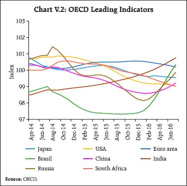 Global trade decelerated further in H1 of 2016 in an environment of subdued demand and rising protectionism, exacerbated by uncertainties surrounding Brexit, the Fed’s monetary policy stance and volatile financial markets (Chart V.3a). While the pace of contraction in trade volume of EMEs reduced markedly in Q2, the slowdown in the trade volume of AEs has continued since Q1 of 2015. Within EMEs, trade volume contracted in all major regions in Q2, except Central and Eastern Europe where weakening currencies have given a significant boost to exports. The pace of contraction reduced sharply in Emerging Asia, with currency depreciation supporting exports in a number of countries, and stimulus driven demand boosting imports in China (Chart V.3b). The World Trade Organisation projects that global trade volume growth in 2016 would be the lowest since the global financial crisis. V.2 Commodity Prices and Global Inflation Global commodity prices have been largely driven by supply conditions even as demand remains soft, barring those of precious metals lifted by safe haven buying. Crude oil prices rallied between January and May on account of supply disruptions in several OPEC countries and North America and a softening of the US dollar, but eased thereafter on the build-up of inventories, particularly in the US. Prices have remained range bound since early September (Chart V.4a). Prices of precious metals have rallied on strong investor demand, weak dollar and safe haven buying. Persistently weak US economic data have been driving up investment demand for precious metals, with Brexit providing a further boost. Post Brexit, gold prices surged to a two-year high and have remained elevated so far. Iron ore prices, which soared in 2016 due to stimulus and property boom driven demand from China, have subsided lately due to increased supply from Brazil and Australia. Food prices have been generally trended upwards since January 2016, with sugar, in particular, showing a sharp increase due to drought in Brazil (Chart V.4b). 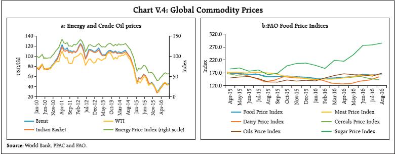 Global Inflationary pressures remain contained by weak global growth and soft commodity prices. In AEs, the general price level remained virtually unchanged despite monetary easing, although core Inflation was firmer (Chart V.5a). In the US, barring medical care and shelter, most of the remaining sectors of the economy faced negative price pressures. In the Euro area, deflation risks increased as the economic outlook deteriorated and business and consumer sentiment weakened, with declining energy prices, strengthening of the euro, subdued wage growth and weak productivity growth accentuating these risks. Japan has also remained in deflation mode for the past five months, induced by faltering consumption and an unrelentingly strong yen. By contrast, Inflation remains diverse among major EMEs. In Brazil, Russia and South Africa, Inflation has been well above the target due to weak currency, food Inflation and structural rigidities, though these pressures have been easing in recent months. On the other hand, China, Korea, Indonesia, Malaysia and Thailand face benign and ebbing Inflationary situations (Chart V.5b). By and large, Inflation in EMEs has benefitted from low commodity prices, ebbing currency depreciation pressures and slack in demand, both at home and abroad (Box V.1). Box V.1: Exchange Rate and Commodity Prices Pass-through to Inflation in EMEs Exchange rate and commodity prices are two important transmission channels of Inflation across open economies. By what percentage Inflation changes in response to a percentage change in exchange rate and commodity prices – the pass-through – is, however, determined by several factors, of which the credibility of monetary policy in anchoring Inflation expectations is an important one (Taylor, 2000). It is imperative to have a good measure of this pass-through in order to understand the Inflationary process and fashion appropriate monetary policy responses. In this context, recent years have seen increased EME currency volatility, driven by policy and political uncertainties emanating from several parts of the globe. There has also been a significant decline in global commodity prices, particularly crude oil, following supply-demand mismatches, though supply disruptions have led to some firming up since January 2016. How much of these currency and commodity prices movements have influenced Inflation in some select EMEs is examined by estimating a reduced form equation derived from a partial equilibrium micro-founded pricing behavior of firms. specifically, the pricing decision of a firm is determined by marginal costs, mark-ups, exchange rate changes, wage costs and income in the exporting and importing countries. In reduced form, this can be specified as:  where, p= consumer prices; e = exchange rate; c = costs; pc = commodity prices (crude oil), y = income (demand) and superscripts d and f are domestic and foreign country, respectively. Estimates carried out in difference form for a panel of 17 EMEs1 employing a battery of estimation methods for the period 2005:Q1 to 2016:Q2 reveal that exchange rates, commodity prices, exporting country’s costs and domestic demand influence Inflation in these EMEs (Table 1). However, the extent of this influence has declined in the post-crisis period, even while Inflation has become more persistent. The pass-through of exchange rate depreciation is far stronger than that of appreciation. Despite the weakening of pass-through, Inflation in EMEs has benefitted from the decline in commodity prices and relative currency stability in the post-crisis period. References: Aron, J., Macdonald, R. and Muellbauer, J. (2014), “Exchange rate pass-through in developing and emerging markets: A survey of conceptual, methodological and policy issues, and selected empirical findings”, Journal of Development Studies, 50(1), pp.101-143. Taylor, B. J. (2000), “Low Inflation, pass-through and the pricing power of firms”, European Economic Review, 44(7), pp. 1389–1408. V.3 Monetary Policy Stance Globally, monetary policy stances remained accommodative in Q2 of 2016. In Q3 so far, some AEs have eased further, as Brexit paralysed markets and added to global uncertainty. The Fed has kept its policy rate unchanged since end-2015; however, in its September meeting, it indicated that the case for a rate hike has strengthened. After pausing for several months, both the UK and Japan have renewed monetary easing as a response to Brexit. The Bank of England cut its policy rate in August and also expanded its asset purchase programme. The Bank of Japan doubled its exchange traded funds (ETF) purchases in July to contain the surge in yen to an almost two year high. In September, it shifted its policy focus from targeting base money to targeting 10-year government bond yields at zero per cent. The ECB has kept its monetary policy stance unchanged since the last cut in the policy rate in March 2016. Monetary policy stances in EMEs have varied. South Korea and Indonesia cut policy rates in Q2, with the latter easing further in September to support the economy as expectations of a rate increase by the US Fed diminished. Russia cut its policy rate by 50 basis points each in June and September on ebbing Inflationary pressures. In contrast, Colombia and Mexico increased policy rates by 200 bps and 150 bps, respectively, during 2016 so far to counter Inflationary pressures emanating from depreciating currencies. Brazil kept its policy rate unchanged in the face of a crippling recession even though Inflation remained well above the target (Charts V.6a & b). V.4 Global Financial Markets Global financial markets rebounded from mid-February through June 23 as positive sentiments prevailed due to continuing accommodative monetary policy stances by central banks in AEs and the widely held expectation that the UK would remain in the European Union. Better than expected global economic conditions, recovery in oil price, stimulus in China, and pushing back of a rate hike by the US Fed reinforced the calm in the financial markets. The unexpected outcome of the Brexit referendum surprised financial markets in June. The initial reactions were severe with large movements in bond yields, equity prices and exchange rates. However, financial markets stabilised quickly, stock markets climbed to intra-year highs in August, and bond yields came off recent lows with volatility easing. Equity markets gained steadily during Q2 of 2016, as risk sentiment improved despite Brexit uncertainties and US economic data providing mixed signals. However, the sharp sell-off around the world triggered by Brexit on June 23 led to a record loss of US$ 3 trillion in market capitalisation in the next two trading days. Volatility surged immediately, but also receded quickly when markets realised that the exit would be a long drawn process. Equity markets subsequently recouped losses, barring UK and European banks. Japanese equity markets rebounded quickly as various measures to stabilise markets were announced. Euro area equity prices, which dropped by around 9 per cent immediately after Brexit, gradually returned to mid-June levels. The impact was less pronounced in the US, as market expected a delay in policy tightening by the Fed even as US payrolls data and corporate earnings beat expectations. EME equity markets performed relatively well in Q2 of 2016 supported by global low policy rates and low volatility. In May, they were impacted by anticipation of a rate hike by the Fed and concerns relating to growth and political risks in some economies. The initial risk-off and flight-to-safety response to the Brexit referendum in June was fully offset by mid- July. In Q3, equity prices have gained by about 4.4 per cent in AEs and 8.3 per cent in EMEs (Chart V.7).  Sovereign bond yields, which had been falling in major AEs, rose in the later part of April due to a global sell-off triggered from Europe, which spread to the US. In May, bond markets traded range-bound, though US treasury securities remained more attractive relative to sovereign securities of other AEs offering negative yields. Post Brexit, increased risk-off behaviour of investors led to a sharp fall in bond yields across major AEs that continued till about mid-July. Thereafter, yields recovered and hardened till mid-September on concerns over major central banks’ ability to continue with unconventional asset purchases. They have recently softened again after the FOMC held rates unchanged in September. Bond yields in EMEs have also eased, buoyed by dovish monetary policy stances of some central banks and rise in commodity prices. Inflows to EME bond markets were modest in May on rising prospects of a Fed rate hike and concerns about growth and political risks in a number of EMEs. However, in June, inflows turned up sharply following dovish signals from the ECB and reduced expectations on tightening by the US Fed, barring some transitory sell-offs around the Brexit referendum. The search for yields in the bond markets of EMEs has further intensified in Q3, with investors taking advantage of record low interest rates in AEs and chasing carry trade. Consequently, yields consistently eased in major EMEs, except in Turkey and South Africa. In currency markets, the divergence in growth and monetary policy in AEs remained the major driving factors. The US dollar depreciated against trading partner currencies during March to late April, largely reflecting revised expectations on the path of the US policy rate. It strengthened subsequently with the widening of long-term bond yield spreads between the US and the Euro area. The appreciation of the yen against major currencies continued through Q2 and Q3, reflecting changing perceptions about monetary policy in Japan vis-a-vis other reserve currencies, and on safe haven flows. The pound sterling, which strengthened against the US dollar in April, started weakening in May on Brexit concerns and fell sharply on the day of the outcome. Since then, it has depreciated by 12.4 per cent against the US dollar (Chart V.8).  Emerging market currencies have remained susceptible to both global and domestic factors. While the Chinese renminbi has depreciated modestly since April, the Turkish lira and the Mexican peso have weakened significantly. The South African rand has turned weaker since mid-August due to economic weakness and escalation of political concerns. By contrast, the Brazilian real gained against the US dollar in Q2 and Q3, driven by global liquidity, bottoming commodity prices and changing domestic political dynamics. The Russian ruble, which rallied between January and June, has stabilised, barring some pressures in mid-July and early August due to bearish oil market conditions and political tensions. In sum, risks to global economic activity and trade are skewed to the downside. While EMEs seem to be recovering, growth in major AEs remains subdued. Inflation is expected to remain benign. Financial markets, despite the recent calm, remain vulnerable to swings in investor sentiment, driven by policy and political uncertainty.
ABBREVIATIONS | ADs | Authorised Dealers | | AEs | Advanced Economies | | ANOVA | Analysis of Variance | | ARCs | Asset Reconstruction Companies | | BBL | Barrel | | BE | Budget Estimates | | BK | Baxter-King | | BPLR | Benchmark Prime Lending Rate | | bps | Basis Points | | BSE | Bombay Stock Exchange | | CACP | Commission for Agricultural Costs and Prices | | CBLO | Collateralised Borrowing and Lending Obligation | | CCEA | Cabinet Committee on Economic Affairs | | CD | Certificate of Deposit | | CF | Christiano-Fitzgerald | | CGA | Controller General of Accounts | | CI | Confidence Interval | | CII | Confederation of Indian Industry | | CMIE | Centre for Monitoring Indian Economy | | CP | Commercial Paper | | CPB | Central Planning Bureau | | CPC | Central Pay Commission | | CPI | Consumer Price Index | | CPI-AL | Consumer Price Index - Agricultural Labourers | | CPI-IW | Consumer Price Index - Industrial Workers | | CPI-RL | Consumer Price Index - Rural Labourers | | CRAR | Capital to Risk Weighted Asset Ratio | | CRR | Cash Reserve Ratio | | CSO | Central Statistics Office | | CVD | Countervailing Duty | | DFM | Dynamic Factor Model | | DGCI&S | Directorate General of Commercial Intelligence and Statistics | | DISCOMs | Distribution Companies | | ECB | European Central Bank | | EMDEs | Emerging Market and Developing Economies | | EMEs | Emerging Market Economies | | ERPT | Exchange Rate Pass-through | | ETF | Exchange Traded Funds | | FAO | Food and Agriculture Organisation | | FCNR(B) | Foreign Currency Non-Resident (Bank) | | FDI | Foreign Direct Investment | | FICCI | Federation of Indian Chambers of Commerce and Industry | | FIMMDA | Fixed Income Money Market and Derivatives Association of India | | FOMC | Federal Open Market Committee | | FPIs | Foreign Portfolio Investors | | FR | Fixed Rate | | FY | Financial Year | | GDP | Gross Domestic Product | | GFCE | Government Final Consumption Expenditure | | GFD | Gross Fiscal Deficit | | GMM | Generalised Method of Moments | | GNDI | Gross National Disposable Income | | GNPA | Gross Non-Performing Assets | | GoI | Government of India | | G-Sec | Government Security | | GST | Goods and Services Tax | | GVA | Gross Value Added | | H1 | First Half of the Year | | H2 | Second Half of the Year | | HP | Hodrick-Prescott | | HQLA | High Quality Liquid Asset | | HRA | House Rent Allowance | | IIP | Index of Industrial Production | | IMF | International Monetary Fund | | INR | Indian Rupee | | IOS | Industrial Outlook Survey | | IPO | Initial Public Offering | | IRC | Insulated Rubber Cables | | kWh | kiloWatt hour | | LAF | Liquidity Adjustment Facility | | LCR | Liquidity Coverage Ratio | | LPA | Long Period Average | | LPG | Liquefied Petroleum Gas | | MCLR | Marginal Cost of Funds Based Lending Rate | | m-o-m | Month-on-Month | | MPC | Monetary Policy Committee | | MPR | Monetary Policy Report | | MSCI | Morgan Stanley Capital International | | MSF | Marginal Standing Facility | | MSP | Minimum Support Price | | MTEF | Medium Term Expenditure Framework | | NCAER | National Council of Applied Economic Research | | NDS-OM | Negotiated Dealing System – Order Matching | | NDTL | Net Demand and Time Liabilities | | NEER | Nominal Effective Exchange Rate | | OD | Overdraft | | OECD | Organisation for Economic Co-operation and Development | | OMCs | Oil Marketing Companies | | OMOs | Open Market Operations | | OPEC | Organisation of the Petroleum Exporting Countries | | OROP | One Rank One Pension | | OTC | Over the Counter | | PE | Price-to-Earnings | | PF | Production Function | | PFCE | Private Final Consumption Expenditure | | PMI | Purchasing Managers’ Index | | POL | Petroleum, Oil and Lubricants | | PPA | Power Purchase Agreement | | PPAC | Petroleum Planning & Analysis Cell | | PRN | Production Weighted Rainfall | | PSB | Public Sector Bank | | PSU | Public Sector Undertaking | | Q | Quarter | | q-o-q | Quarter-on-Quarter | | RBI | Reserve Bank of India | | REER | Real Effective Exchange Rate | | RHS | Right Hand Side | | RMSE | Root Mean Square Error | | RNR | Revenue Neutral Rate | | RW | Random Walk | | SAAR | Seasonally Adjusted Annualised Rate | | SCB | Scheduled Commercial Bank | | SD | Standard Deviation | | SEBI | Securities and Exchange Board of India | | SLR | Statutory Liquidity Ratio | | UDAY | Ujwal DISCOM Assurance Yojana | | UK | United Kingdom | | US | United States | | US$ | Unites States Dollar | | VAR | Vector Auto Regression | | VDA | Variable Dearness Allowance | | VR | Variable Rate | | WACR | Weighted Average Call Money Rate | | WALR | Weighted Average Lending Rate | | WMA | Ways and Means Advances | | WPI | Wholesale Price Index | | WTO | World Trade Organisation | | y-o-y | Year-on-Year | |