A.2.1 Corporate sector Corporate sector stability indicator and map The corporate sector stability indicator and map have been constructed using the following method: Data: The balance sheet data of non-government non-financial (NGNF) companies. Frequency: Annual (1992-93 to 2011-12). From 2012-13 to 2016-17, the half-yearly balance sheet data is used for the analysis. The ratios used under each dimensions are given in the Table A.2.1. | Table A.2.1: Ratios used for constructing the corporate sector stability map and indicator | | Dimensions | Ratios | | Profitability | RoA (Gross Profit/Total Assets)#, Operating Profit/Sales#, Profit After Tax/Sales# | | Leverage | Debt/ Assets, Debt/ Equity; (Debt is taken as Total Borrowings) | | Sustainability | Interest Coverage Ratio (EBIT to interest expenses)#, interest expenses/total expenditure; | | Liquidity | Quick Assets/ Current Liabilities (quick ratio)#; | | Turn-Over | Total Sales / Total Assets#. | | # Negatively related to risk. | Each ratio (Xt) was normalised for the sample period using relative distance transformation given below: For (#) negatively related ratios (to risk), one’s complement was used. For each dimension a composite index was derived as a simple average of relevant d’s (principal component analysis (PCA) also gives equal weights). The Map is constructed using composite index for each dimension. The overall corporate sector stability indicator is a weighted average of 5 dimensions. The weights are obtained using PCA. The derived weights for five dimensions are as follows: | Profitability | Leverage | Sustainability | Liquidity | Turn-Over | | 25% | 25% | 25% | 10% | 15% | Sensitivity Analysis-Stress test The resilience of the NGNF listed companies to potential shocks to domestic interest rates and operating profits were assessed using sensitivity tests. A set of common companies were taken for three years. The tests were done for the following three scenarios: Scenario 1: Operating profit decreased by 25 per cent. Scenario 2: Domestic interest rates increased by 250 basis points (bps). Scenario 3: Combined effect of the above two scenarios. The number of weak and weak leveraged companies and share of debt of such companies in the total debt of all companies in the sample were calculated by imparting shocks on half-yearly balance sheet and profit and loss statements of each company for the last three half years. In scenario 1, the operating profit is decreased by 25 per cent, which impacted the earnings before interest, tax and depreciation (EBITDA). This resulted in a decline in earnings before taxes (EBT) and thus lowered the provisions. Tax provision is decreased by using tax by EBT ratio for companies reporting positive EBT. Tax provisions of companies reporting negative EBT were not adjusted. The decline in net profits is adjusted in the reserves and surplus of the balance sheet. Under scenario 2, the cost of borrowings of each company is computed using interest payable to the average total borrowings of the companies. Cost of borrowings of each company is increased by 250 bps and the increased interest expenses is computed. Increase in interest expenses resulted in decline in EBT. The tax provision and reserve and surplus were adjusted using the same procedure as described in scenario 1. A.2.2 Scheduled commercial banks Banking stability map and indicator The banking stability map and indicator present an overall assessment of changes in underlying conditions and risk factors that have a bearing on the stability of the banking sector during a period. The five composite indices used in the banking stability map and indicator represent the five dimensions of soundness, asset-quality, profitability, liquidity and efficiency. The ratios used for constructing each composite index are given in Table A.2.2. | Table A.2.2: Ratios used for constructing the banking stability map and indicator | | Dimension | Ratios | | Soundness | CRAR # | Tier-I Capital to Tier-II Capital # | Leverage Ratio as Total-Assets to Capital and Reserves | | Asset- Quality | Net NPAs to Total- Advances | Gross NPAs to Total- Advances | Sub-Standard-Advances to Gross NPAs # | Restructured-Standard- Advances to Standard- Advances | | Profitability | Return on Assets # | Net Interest Margin # | Growth in Profit # | | Liquidity | Liquid-Assets to Total-Assets # | Customer-Deposits to Total-Assets # | Non-Bank-Advances to Customer-Deposits | Deposits maturing within-1-year to Total Deposits | | Efficiency | Cost to Income | Business (Credit + Deposits) to Staff Expenses # | Staff Expenses to Total Expenses | | Note: # Negatively related to risk. | Each composite index, representing a dimension of bank functioning, takes values between zero and 1. Each index is a relative measure during the sample period used for its construction, where a higher value means the risk in that dimension is high. Therefore, an increase in the value of the index in any particular dimension indicates an increase in risk in that dimension for that period as compared to other periods. For each ratio used for a dimension, a weighted average for the banking sector is derived, where the weights are the ratio of individual bank assets to total banking system assets. Each index is normalised for the sample period using the following formula: 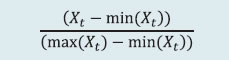 Where, Xt is the value of the ratio at time t. A composite index of each dimension is calculated as a weighted average of normalised ratios used for that dimension where the weights are based on the marks assigned for assessment for the CAMELS rating. The banking stability indicator is constructed as a simple average of these five composite indices. Macro-stress testing To ascertain the resilience of banks against macroeconomic shocks, a macro-stress test for credit risk was conducted. Under this, the impact of macro shock on GNPAs ratio of banks (at system and major bank-groups level) and finally on their capital adequacy (bank-by-bank and system level for the sample of 55 banks) were seen. Impact of GNPA ratio Here, the slippage ratio (SR)1 was modelled as a function of macroeconomic variables, using various econometric models that relate the select banking system aggregates to macroeconomic variables. The time series econometric models used were: (i) multivariate regression to model system level slippage ratio; (ii) Vector Autoregression (VAR) to model system level slippage ratio; (iii) quantile regression to model system level slippage ratio; (iv) multivariate regression to model bank group-wise slippage ratio; and (v) VAR to model bank group-wise slippage ratio. The banking system aggregates include current and lagged values of slippage ratio, while macroeconomic variables include real gross value added (GVA) at basic price growth, weighted average lending rate (WALR), CPI (combined) inflation, exports-to-GDP ratio (EXGDP), current account balance to GDP ratio (CABGDP) and gross fiscal deficit-to-GDP ratio (GFDGDP). While multivariate regression allows evaluating the impact of select macroeconomic variables on the banking system’s asset quality, the VAR model also takes into account the feedback effect. In these methods, the conditional mean of slippage ratio is estimated and it is assumed that the impact of macro-variables on credit quality will remain the same irrespective of the level of the credit quality, which may not always be true. In order to relax this assumption, quantile regression was adopted to project credit quality, wherein conditional quantile was estimated instead of the conditional mean and hence it can deal with tail risks and takes into account the non-linear impact of macroeconomic shocks. The following econometric models were used to estimate the impact of macroeconomic shocks on the slippage ratio: System level models The system level GNPAs were projected using three different but complementary econometric models: multivariate regression, VAR and quantile regression. The average of projections derived from these models was presented. • Multivariate regression The analysis was carried out on the slippage ratio at the aggregate level for the commercial banking system as a whole. • VAR model In notational form, mean-adjusted VAR of order p (VAR(p)) can be written as: In order to estimate the VAR model, slippage ratio, WALR, CPI (combined) inflation, GVA at basic price growth and gross fiscal deficit-to-GDP ratio were selected. The appropriate order of VAR was selected based on minimum information criteria as well as other diagnostics and suitable order was found to be 2. The impact of various macroeconomic shocks was determined using the impulse response function of the selected VAR. • Quantile regression In order to estimate the conditional quantile of slippage ratio at 0.8, the following quantile regression was used: Bank group level models The bank groups-wise SR were projected using two different but complementary econometric models: multivariate regression and VAR. The average of projections derived from these models was presented. • Multivariate regression In order to model the slippage ratio of various bank groups, the following multivariate regressions for different bank groups were used: Public Sector Banks (PSBs): Private Sector Banks (PVBs): Foreign Banks (FBs): Where, dummy is time dummy. • VAR model In order to model the slippage ratio of various bank groups, different VAR models of different orders were estimated based on the following macro variables: PSBs: GVA at basic price growth, CPI (combined)-inflation, WALR, CAB to GDP Ratio and GFD to GDP ratio of order 2. PVBs: GVA at basic price growth, real WALR and Exports to GDP ratio of order 1. FB: CPI (combined)-inflation, WALR and CAB to GDP ratio of order 2. Estimation of GNPAs from slippages Once, slippage ratio is projected using above mentioned models, the GNPA is projected using the identity given below: GNPAT+1=GNPAT + Slippage(T,T+1) – Recovery(T,T+1) – Write-off(T,T+1) – Upgradation(T,T+1) Derivation of GNPAs from slippage ratios, which were projected from the above mentioned credit risk econometric models, were based on the following assumptions: credit growth of 7 per cent; recovery rate of 3.6 per cent, 2.7 per cent, 3.3 per cent and 2.3 per cent during March, June, September and December quarters respectively; write-off rates of 4.5 per cent, 4.1 per cent, 4.0 per cent and 3.9 per cent during March, June, September and December respectively; Up-gradation rates of 2.9 per cent, 3.2 per cent, 2.9 per cent and 2.5 per cent during March, June, September and December respectively. Impact on capital adequacy The impact of macro shocks on capital adequacy of banks was captured through the following steps; i. The impact on future capital accumulation was captured through projection of profit under the assumed macro scenarios, assuming that only 25 per cent of profit after tax (PAT) (which is minimum regulatory requirements) goes into capital of banks. ii. The requirement of additional capital in future and macro stress scenarios were projected through estimating risk-weighted assets (RWAs) using internal rating-based (IRB) formula. The formulas used for the projection of capital adequacy are given below: Where, PAT is projected using satellite models which are explained in the subsequent section. RWAs (others), which is total RWAs minus RWAs of credit risk, was projected based on average growth rate observed in the past one year. RWAs (credit risk) is estimated using the IRB formula given below: IRB Formula: Bank-wise RWAs for credit risk were estimated using the following IRB formula; Where, EADi is exposure at defaults of the bank in the sector i (i=1,2….n). Ki is minimum capital requirement for the sector i which is calculated using the following formula: Where, LGDi is loss given default of the sector i, PDi is probability of default of the sector i, N(..) is cumulative distribution function of standard normal distribution, G(..) is inverse of cumulative distribution function of standard normal distribution, Mi is average maturity of loans of the sector (which is taken 2.5 for all the sector in this case), b(PDi) is smoothed maturity adjustment and Ri is correlation of the sector i with the general state of the economy. Calculation of both, b(PD) and R depend upon PD. The above explained IRB formula requires three major inputs, namely, sectoral PD, EAD and LGD. Here, sectoral PDs was proxies by annual slippage of the respective sectors using banking data. PD for a particular sector was taken as same (i.e. systemic shocks) for each sample of 55 selected banks, whereas, EAD for a bank for a particular sector was total outstanding loan (net of NPAs) of the bank in that particular sector. Further, assumption on LGD was taken as follows; under the baseline scenario, LGD = 60 per cent (broadly as per the RBI guidelines on ‘Capital Adequacy – The IRB Approach to Calculate Capital Requirement for Credit Risk’), which increases to 65 per cent under medium macroeconomic risk scenario and 70 per cent under severe macroeconomic risk. Selected sectors: The following 17 sectors (and others) selected for the stress test. | Table A.2.3: List of selected sectors | | Sr. No. | Sector | Sr. No. | Sector | | 1 | Engineering | 10 | Basic Metal and Metal Products | | 2 | Vehicles, Parts and Transport Equipments | 11 | Mining | | 3 | Cement | 12 | Paper | | 4 | Chemicals | 13 | Petroleum | | 5 | Construction | 14 | Agriculture | | 6 | Textiles | 15 | Retail-Housing | | 7 | Food Processing | 16 | Retail-Others | | 8 | Gems and Jewellery | 17 | Services | | 9 | Infrastructure | 18 | Others | The stochastic relationship of sectoral annual slippage ratio (i.e. sectoral PDs) with macro variables was estimated using multivariate regression for each sector. Using these estimated regressions, sectoral PDs of each sector were projected for upto four quarters ahead under assumed baseline as well as two adverse scenarios, namely, medium stress and severe stress. The sectoral regression models are presented in the next section. In order to project capital adequacy under assumed macro scenarios, credit growth on y-o-y basis was assumed which was based on the trend observed in the last two years. The bank-wise PAT was projected using the following steps: • Components of PAT (i.e. net interest income, other operating income, operating expenses and Provisions) of each bank-groups were projected under baseline and adverse scenarios using the method explained in the subsequent section. • Share of components of PAT of each banks (except income tax) in their respective bank-group was calculated. • Each components of PAT (except income tax) of each bank were projected from the projected value of component of PAT of respective bank-group and applying that bank’s share in the particular component of PAT. • Finally, bank-wise PAT was projected by appropriately adding or subtracting their components estimated in the previous step and using rate of income tax at 35 per cent. Using the above formulas, assumptions and inputs, impact of assumed macro scenarios on the capital adequacy at bank level was estimated and future change in capital adequacy under baseline from the latest actual observed data and changed in the capital adequacy of banks from baseline to adverse macro shocks were calculated. Finally, these changes appropriately applied on the latest observed capital adequacy (under Standardised Approach) of the bank. Projection of Sectoral PDs Projection of bank-group wise PAT The various components of PAT of major bank-groups (namely, PSBs, PVBs and FBs), like, interest income, other income, operating expenses and provisions were projected using different time series econometric models (as given below). Finally, PAT was estimated using the following identity: Where, NII is net interest income, OOI is other operating income and OE is operating expenses. Net Interest Income (NII): NII is the difference between interest income and interest expense and was projected using the following regression model: LNII is log of NII. LNGDP_SA is seasonally adjusted log of nominal GDP. Adv_Gr is the y-o-y growth rate of advances. Spread is the difference between average interest rate earned by interest earning assets and average interest paid on interest bearing liabilities. Other Operating Income (OOI): The OOI of SCBs was projected using the following regression model: LOOI is log of OOI. Operating Expense (OE): The OE of SCBs was projected using the Autoregressive Moving Average (ARMA) model. Provision: The required provisioning was projected using the following regression: P_Adv is provisions to total advances ratio. RGVA_Gr is the y-o-y growth rate of real GVA. GNPA is gross nonperforming advances to total advances ratio and hence impact of deteriorated asset quality under assumed macro shocks on income is captured this equation. Dummy is a time dummy. Income Tax: The applicable income tax was taken as 35 per cent of profit before tax, which is based on the past trend of ratio of income tax to profit before tax Single factor sensitivity analysis – Stress testing As a part of quarterly surveillance, stress tests are conducted covering credit risk, interest rate risk, liquidity risk etc. and the resilience of commercial banks in response to these shocks is studied. The analysis is done on individual SCBs as well as on the system level. Credit risk To ascertain the resilience of banks, the credit portfolio was given a shock by increasing GNPA levels for the entire portfolio as well as for few select sectors. For testing the credit concentration risk, default of the top individual borrower(s) and the largest group borrower(s) for each individual bank was assumed. The analysis was carried out both at the aggregate level as well as at the individual bank level. The assumed increase in GNPAs was distributed across sub-standard, doubtful and loss categories in the same proportion as prevailing in the existing stock of NPAs. However, for credit concentration risk the additional GNPAs under the assumed shocks were considered to fall into sub-standard category only. The provisioning norms used for these stress tests were based on existing average prescribed provisioning for different asset categories. The provisioning requirements were taken as 25 per cent, 75 per cent and 100 per cent for substandard, doubtful and loss advances respectively. These norms were applied on additional GNPAs calculated under a stress scenario. As a result of the assumed increase in GNPAs, loss of income on the additional GNPAs for one quarter was also included in total losses, in addition to the incremental provisioning requirements. The estimated provisioning requirements so derived were deducted from banks’ capital and stressed capital adequacy ratios were computed. Interest rate risk Under assumed shocks of the shifting of the INR yield curve, there could be losses on account of the fall in value of the portfolio or decline in income. These estimated losses were reduced from the banks’ capital to arrive at stressed CRAR. For interest rate risk in the trading portfolio (HFT + AFS), a duration analysis approach was considered for computing the valuation impact (portfolio losses). The portfolio losses on these investments were calculated for each time bucket based on the applied shocks. The resultant losses/gains were used to derive the impacted CRAR. In a separate exercise for interest rate shocks in the HTM portfolio, valuation losses were calculated for each time bucket on interest bearing assets using the duration approach. The valuation impact for the tests on the HTM portfolio was calculated under the assumption that the HTM portfolio would be marked-to-market. Evaluation of the impact of interest rate risk on the banking book was done through the ‘income approach’. The impact of shocks were assessed by estimating income losses on the exposure gap of rate sensitive assets and liabilities, excluding AFS and HFT portfolios, for one year only for each time bucket separately. This reflects the impact on the current year profit and loss. Equity price risk Under the equity price risk, impact of a shock of a fall in the equity price index, by certain percentage points, on profit and bank capital were examined. The fall in value of the portfolio or income losses due to change in equity prices are accounted for the total loss of the banks because of the assumed shock. The estimated total losses so derived were reduced from the banks’ capital. Liquidity risk The aim of the liquidity stress tests is to assess the ability of a bank to withstand unexpected liquidity drain without taking recourse to any outside liquidity support. Various scenarios depict different proportions (depending on the type of deposits) of unexpected deposit withdrawals on account of sudden loss of depositors’ confidence along with a demand for unutilised portion of sanctioned/committed/ guaranteed credit lines (taking into account the undrawn working capital sanctioned limit, undrawn committed lines of credit and letters of credit and guarantees). The stress tests were carried out to assess banks’ ability to fulfil the additional and sudden demand for credit with the help of their liquid assets alone. Assumptions used in the liquidity stress tests are given below: • It is assumed that banks will meet stressed withdrawal of deposits or additional demand for credit through sale of liquid assets only. • The sale of investments is done with a haircut of 10 per cent on their market value. • The stress test is done under a ‘static’ mode. Bottom-up stress testing: Select banks Bottom-up sensitivity analysis was performed by 25 select scheduled commercial banks. A set of common scenarios and shock sizes were provided to the select banks. The tests were conducted using March 2017 data. Banks used their own methodologies for calculating losses in each case. Bottom-up stress testing: Derivatives portfolios of select banks The stress testing exercise focused on the derivatives portfolios of a representative sample set of top 22 banks in terms of notional value of the derivatives portfolios. Each bank in the sample was asked to assess the impact of stress conditions on their respective derivatives portfolios. In case of domestic banks, the derivatives portfolio of both domestic and overseas operations was included. In case of foreign banks, only the domestic (Indian) position was considered for the exercise. For derivatives trade where hedge effectiveness was established it was exempted from the stress tests, while all other trades were included. The stress scenarios incorporated four sensitivity tests consisting of the spot USD/INR rate and domestic interest rates as parameters | Table A.2.4: Shocks for sensitivity analysis | | | Domestic interest rates | | Shock 1 | Overnight | +2.5 percentage points | | Up to 1yr | +1.5 percentage points | | Above 1yr | +1.0 percentage points |
| | Domestic interest rates | | Shock 2 | Overnight | -2.5 percentage points | | Up to 1yr | -1.5 percentage points | | Above 1yr | -1.0 percentage points |
| | Exchange rates | | Shock 3 | USD/INR | +20 per cent |
| | Exchange rates | | Shock 4 | USD/INR | -20 per cent | A.2.3 Scheduled urban co-operative banks Single factor sensitivity analysis – Stress testing Credit risk Stress tests on credit risk were conducted on scheduled urban co-operative banks (SUCBs). The tests were based on a single factor sensitivity analysis. The impact on CRAR was studied under following four different scenarios, using the historical standard deviation (SD). • Scenario I: 1 SD shock on GNPA (classified into sub-standard advances). • Scenario II: 2 SD shock on GNPA (classified into sub-standard advances). • Scenario III: 1 SD shock on GNPA (classified into loss advances). • Scenario IV: 2 SD shock on GNPA (classified into loss advances). Liquidity risk A liquidity stress test based on a cash flow basis in the 1-28 days time bucket was also conducted, where mismatch [negative gap (cash inflow less cash outflow)] exceeding 20 per cent of outflow was considered stressful. • Scenario I: Cash outflows in the 1-28 days time bucket goes up by 50 per cent (no change in cash inflows). • Scenario II: Cash outflows in the 1-28 days time bucket goes up by 100 per cent (no change in cash inflows). Non-banking financial companies Single factor sensitivity analysis – Stress testing Credit risk Stress tests on credit risk were conducted on non-banking financial companies (including both deposit taking and non-deposit taking and systemically important). The tests were based on a single factor sensitivity analysis. The impact on CRAR was studied under three different scenarios, based on historical SD: • Scenario I: GNPA increased by 0.5 SD from the current level. • Scenario II: GNPA increased by 1 SD from the current level. • Scenario III: GNPA increased by 3 SD from the current level. The assumed increase in GNPAs was distributed across sub-standard, doubtful and loss categories in the same proportion as prevailing in the existing stock of GNPAs. The additional provisioning requirement was adjusted from the current capital position. The stress test was conducted at individual NBFC level as well as at the aggregate level. A.2.5 Interconnectedness – Network analysis Matrix algebra is at the core of the network analysis, which uses the bilateral exposures between entities in the financial sector. Each institution’s lendings to and borrowings from all other institutions in the system are plotted in a square matrix and are then mapped in a network graph. The network model uses various statistical measures to gauge the level of interconnectedness in the system. Some of the important measures are given below: 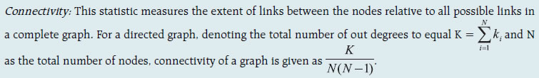 Cluster coefficient: Clustering in networks measures how interconnected each node is. Specifically, there should be an increased probability that two of a node’s neighbours (banks’ counterparties in case of a financial network) are neighbours to each other also. A high clustering coefficient for the network corresponds with high local interconnectedness prevailing in the system. For each bank with ki neighbours the total number of all possible directed links between them is given by ki (ki-1). Let Ei denote the actual number of links between agent i’s ki neighbours, viz. those of i’s ki neighbours who are also neighbours. The clustering coefficient Ci for bank i is given by the identity: Shortest path length: This gives the average number of directed links between a node and each of the other nodes in the network. Those nodes with the shortest path can be identified as hubs in the system. In-betweeness centrality: This statistic reports how the shortest path lengths pass through a particular node. Eigenvector measure of centrality: Eigenvector centrality is a measure of the importance of a node (bank) in a network. It describes how connected a node’s neighbours are and attempts to capture more than just the number of out degrees or direct ‘neighbours’ that a node has. The algorithm assigns relative centrality scores to all nodes in the network and a nodes centrality score is proportional to the sum of the centrality scores of all nodes to which it is connected. For a NxN matrix there will be N different eigen values, for which an eigenvector solution exists. Each bank has a unique eigen value, which indicates its importance in the system. This measure is used in the network analysis to establish the systemic importance of a bank and by far it is the most crucial indicator. Tiered network structures: Typically, financial networks tend to exhibit a tiered structure. A tiered structure is one where different institutions have different degrees or levels of connectivity with others in the network. In the present analysis, the most connected banks (based on their eigenvector measure of centrality) are in the innermost core. Banks are then placed in the mid-core, outer core and the periphery (the respective concentric circles around the centre in the diagrams), based on their level of relative connectivity. The range of connectivity of the banks is defined as a ratio of each bank’s in degree and out degree divided by that of the most connected bank. Banks that are ranked in the top 10 percentile of this ratio constitute the inner core. This is followed by a mid-core of banks ranked between 90 and 70 percentile and a 3rd tier of banks ranked between the 40 and 70 percentile. Banks with a connectivity ratio of less than 40 per cent are categorised as the periphery. Colour code of the network chart: The blue balls and the red balls represent net lender and net borrower banks respectively in the network chart. The colour coding of the links in the tiered network diagram represents the borrowing from different tiers in the network (for example, the green links represent borrowings from the banks in the inner core). Solvency contagion analysis The contagion analysis is in nature of stress test where the gross loss to the banking system owing to a domino effect of one or more banks failing is ascertained. We follow the round by round or sequential algorithm for simulating contagion that is now well known from Furfine (2003).2 Starting with a trigger bank i that fails at time 0, we denote the set of banks that go into distress at each round or iteration by Dq, q= 1,2, …For this analysis, a bank is considered to be in distress when its Tier I CRAR goes below 7 per cent. The net receivables have been considered as loss for the receiving bank. Liquidity contagion analysis While the solvency contagion analysis assesses potential loss to the system owing to failure of a net borrower, liquidity contagion estimates potential loss to the system due to the failure of a net lender. The analysis is conducted on gross exposures between banks. The exposures include fund based and derivatives ones. The basic assumption for the analysis is that a bank will initially dip into its liquidity reserves or buffers to tide over a liquidity stress caused by the failure of a large net lender. The items considered under liquidity reserves are: (a) excess CRR balance; (b) excess SLR balance; and (c) available marginal standing facility. If a bank is able to meet the stress with liquidity buffers alone, then there is no further contagion. However, if the liquidity buffers alone are not sufficient, then a bank will call in all loans that are ‘callable’, resulting in a contagion. For the analysis only short-term assets like money lent in the call market and other very short-term loans are taken as callable. Following this, a bank may survive or may be liquidated. In this case there might be instances where a bank may survive by calling in loans, but in turn might propagate a further contagion causing other banks to come under duress. The second assumption used is that when a bank is liquidated, the funds lent by the bank are called in on a gross basis, whereas when a bank calls in a short-term loan without being liquidated, the loan is called in on a net basis (on the assumption that the counterparty is likely to first reduce its short-term lending against the same counterparty). Joint solvency-liquidity contagion analysis A bank typically has both positive net lending positions against some banks while against some other banks it might have a negative net lending position. In the event of failure of such a bank, both solvency and liquidity contagion will happen concurrently. This mechanism is explained by the following flowchart: The trigger bank is assumed to have failed for some endogenous reason, i.e., it becomes insolvent and thus impacts all its creditor banks. At the same time it starts to liquidate its assets to meet as much of its obligations as possible. This process of liquidation generates a liquidity contagion as the trigger bank starts to call back its loans. The lender/creditor banks that are well capitalised will survive the shock and will generate no further contagion. On the other hand, those lender banks whose capital falls below the threshold will trigger a fresh contagion. Similarly, the borrowers whose liquidity buffers are sufficient will be able to tide over the stress without causing further contagion. But some banks may be able to address the liquidity stress only by calling in short term assets. This process of calling in short term assets will again propagate a contagion. The contagion from both the solvency and liquidity side will stop/stabilise when the loss/shocks are fully absorbed by the system with no further failures.
|