Public finances of states deteriorated in 2013-14 and 2014-15 (RE). While revenue receipts slowed in 2013-14 as overall economic activity slackened, they were shored up in 2014-15 by grants in aid through enhanced transfers under ‘State Plan Schemes’. Despite higher devolution of taxes, central transfers-GDP ratio is budgeted to decline in 2015-16 due to discontinuation of many centrally sponsored schemes (CSSs). Expenditure rationing measures have been budgeted to arrest the erosion in state finances in 2015-16 (BE), but adverse implications for the quality of consolidation raise concerns.

1. Introduction

3.1 Against the backdrop of some slippages in key deficit indicators during 2013-14 and 2014-15 (RE), most states have budgeted for reverting back to the path of fiscal consolidation in 2015-16 (BE). This is sought to be achieved by increasing the surplus in the revenue account and a marginal decline in capital outlay (as a proportion to GDP) (Table III.1).

2. Accounts: 2013-14

3.2 The fiscal position of states deteriorated during 2013-14, leading to re-emergence of a revenue deficit (RD) after a gap of three years (Table III.1).² The reduction in consolidated revenue expenditure was more than offset by a reduction in revenue receipts, reflecting the slowdown in overall economic activity. The fiscal position of both special category (SC) and non-special category (NSC) states deteriorated, although the SC states continued to post a modest surplus (Table III.2).

3.3 The consolidated revenue receipts-GDP ratio of states declined due to reduction in both own revenue and central transfers (Table III.3). In particular, revenue from stamps and registration fees, sales tax/value added tax (VAT) and state excise as well as shares in central taxes decelerated in 2013-14 from a year ago (Table III.4). On the other hand, debt receipts have increased (Table III.3).

3. Revised Estimates: 2014-15

3.4 Latest available data show an increase in states’ consolidated capital outlay-GDP ratio and a deterioration in the GFD-GDP ratio in 2014-15 (RE). The increase in revenue receipts was commensurate with the increase in revenue expenditure resulting in an unchanged revenue deficit from 2013-14 which, however, exceeded the budgeted level for 2014-15.

The revenue accounts of 14 states deteriorated while the GFD-GSDP ratio worsened in 23 states.

3.5 A sharp increase in central transfers in 2014-15 reflected the year-on-year increase by 1.3 per cent of GDP in grants from the Centre for state plan schemes. This reflected the changing pattern of funding for CSS.³

3.6 Revenue expenditure increased significantly during 2014-15 on account of higher expenditure on certain social and economic services (Table III.5).⁴ Education, sports, art and culture and rural development received higher disbursements. Non-development revenue expenditure also increased, primarily due to the increase in administrative services and pensions. Interest payments remained unchanged in 2014-15.⁵

3.7 Capital outlay increased significantly in 2014-15 over the previous year. Expenditure on social services such as education, sports, art and culture, medical and public health, water supply and sanitation, housing and economic services viz., food storage and warehousing and rural development also accelerated during the year.

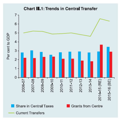
4. Budget Estimates: 2015-16

Key Deficit Indicators

3.8 All key deficit indicators are budgeted to improve in 2015-16 at the aggregate level. The consolidated revenue account of state governments is projected to be in surplus during 2015-16, indicative of the intent to resume fiscal consolidation. An improvement in the revenue account and a marginal decline in capital outlay is expected to provide the necessary fiscal space for a reduction in the GFD-GDP ratio by 0.5 percentage point from its level a year ago. A reduction of 0.6 percentage point in the primary deficit is envisaged, which is conducive for long-run sustainability of state finances.

3.9 While 20 states have budgeted for revenue surplus, 18 have budgeted for improvements in their revenue accounts in terms of GSDP. The GFD and the PD are budgeted to decline in 16 and 17 states, respectively (Table III.6).

3.10 The FC-XIV suggested a ceiling for states’ GFD at 3 per cent of GSDP for the award period. An additional borrowing limit of 0.25 per cent each was allowed if (i) states’ debt-GSDP is less than or equal to 25 per cent and/or (ii) interest payment/ revenue receipts are less than or equal to 10 per cent. These two options can be availed by a state either separately or simultaneously if both criteria are fulfilled. Thus, a state can effectively have a maximum GFD-GSDP limit of 3.5 per cent in a year. Availing additional borrowing is contingent upon the state recording a zero revenue deficit in the year for which the borrowing limit has to be fixed and the immediately preceding year.

Gross Fiscal Deficit

3.11 Market borrowings would continue to remain the major source of financing the GFD of states, with its share set to increase significantly. Over the years, the contribution of public account items like ‘deposits and advances’ and ‘suspense and miscellaneous’ in GFD financing has declined (Table III.7).

Revenue Receipts

3.12 The decline in consolidated central transfers is budgeted to counterbalance the marginal increase in states’ own revenue receipts, resulting in a lower revenue receipts-GDP ratio. Despite an increase in the share of tax devolution from 32 per cent to 42 per cent of the divisible pool on the recommendations of the FC-XIV, the central transfers-GDP ratio is budgeted to decline due to the sharp reduction in grants-in-aid. This could be an outcome of discontinuation of many CSS schemes in the Union Budget 2015-16, resulting in a decline of funds under the state plan scheme.⁶ Instead of increasing the funds available to state governments, these changes have led to a decline in central transfers to states by 0.3 per cent of GDP (Chart III.1).

Expenditure Pattern

3.13 The consolidated revenue expenditure-GDP ratio of state governments is budgeted to be smaller by 0.7 percentage points due to lower growth in its developmental component (both social and economic services). Almost all heads of development revenue expenditure under social and economic services are budgeted to grow at a slower pace in 2015-16 than a year ago. There has been a decline in projected (absolute terms) revenue expenditure for important items such as housing, urban development, soil and water conservation, rural development, irrigation and flood control and energy, which is a cause for concern. On the other hand, committed expenditure is budgeted to marginally increase in 2015-16, primarily due to rise in pension liabilities. The increase in committed expenditure is higher for special category states vis-a-vis the non-special category.

3.14 Capital expenditure⁷ is budgeted to decelerate in 2015-16. The major concern is not only the deceleration of developmental capital outlay on social and economic services, but an absolute decline in capital outlay on services like family welfare, water supply and sanitation, housing, food storage and warehousing, industry and minerals and science, technology and environment.

3.15 As a consequence, social sector expenditure (SSE), which had increased in 2014-15, is budgeted to decline in 2015-16 in as many as 21 states (Chart III.2 and Table III.8). This does not augur well for the quality of human development.

5. Outstanding Liabilities of State Governments

3.16 The outstanding liabilities of state governments have experienced double digit growth since 2012-13 (Table III.9). However the consolidated debt – GDP ratio remains below the target recommended by FC-XIII for states (Table III.10). SC states continue to confront geographical constraints which not only impact their expenditure through higher costs but also inhibit their revenue raising capacity, notwithstanding higher grants from the Centre.

These features of SC states impart downward rigidities to their GFD and debt ratios.

3.17 Despite the budgeted reduction in GFD-GDP ratio in 2015-16, outstanding liabilities would increase on account of the phased takeover of bonds issued by power discoms under the Financial Restructuring Plan (FRP). As the participating states in the FRP would have to progressively take over the entire bond liabilities of the discoms by extending guarantees by 2017-18, their liabilities would increase in the coming years. In this regard, the new initiative of the Government to financially turnaround discoms – Ujjwal Discom Assurance Yojana (UDAY) – may likely alleviate the non-performing asset (NPA) problem of banks, but would increase the liabilities of participating states (See Box IV.1 in Chapter IV).

Composition of Debt

3.18 Outstanding liabilities of states’ reveal the steady increase in market borrowings in recent years (Tables III.11). A steady decline in net collections under NSSF combined with increasing repayment obligations has resulted in a decline in fresh investments by NSSF in state government special securities. Similarly, states’ dependence on loans from the Centre continued to decline.

3.19 The weighted average interest rate on state government securities moderated to 8.28 per cent in 2015-16 from 8.58 per cent in 2014-15. The interest rate spreads over the benchmark 10-year central government security were in the range of 21-109 basis points in 2015-16 vis-a-vis 20-57 basis points in 2014-15. The weighted average spread at 50 basis points in 2015-16 was higher than that in 2014-15 (38 basis points). Among the states, Odisha and Himachal Pradesh issued securities of less than 10 years maturity while Gujarat issued security for 15 years in 2015-16.

Maturity Profile of State Government Securities

3.20 At the end of March 2015 around 68.5 per cent of state development loans (SDLs) were in the maturity bucket of five years and above⁸ (Table III.12). The increase in market borrowings of state governments since 2008-09 entails large repayment obligations from 2017-18 onwards.

Liquidity Position and Cash Management

3.21 Several state governments have been accumulating sizeable cash surpluses in recent years. Liquidity pressures during 2015-16 were thus confined to only a few states. While states’ intermediate treasury bills (ITB) balance was higher at ₹1492.42 billion as on March 31, 2016 (provisional data) as against ₹841.85 billion a year ago, balances on auction treasury bills (ATB) were lower at ₹383.28 billion as against ₹394.26 billion.

3.22 The magnitude of availment of ways and means advances (WMA) and overdrafts (ODs) was marginally higher in 2015-16 than in the previous year notwithstanding intermittent fluctuations (Chart III.3). The WMA scheme has been periodically reviewed, keeping in view states’ requirements, evolving fiscal, financial and institutional developments as well as the objectives of monetary and fiscal management. In this context, an Advisory Committee (Chairman: Shri Sumit Bose) reviewed the existing WMA scheme for state governments, particularly the formula for fixation of limits, and submitted its report on November 20, 2015. Based on the recommendations of the Committee, the aggregate WMA limit for all state governments were increased from ₹153.60 billion to ₹322.25 billion effective February 1, 2016. These limits would continue for two years.

6. Conclusion

3.23 The fiscal health of states deteriorated in 2013-14 with their consolidated revenue account turning into a deficit after a gap of three years. States’ fiscal situation further weakened in 2014-15 (RE) as GFD and PD increased as proportions to GDP. The overall fiscal performance of states is expected to improve with the revenue account turning back to surplus thus enabling a reduction in GFD-GDP ratio during 2015-16. Such improvement, if sustained, would reduce the debt burden of states and facilitate their progress on the path of fiscal consolidation.

¹ The analysis of various fiscal indicators is in proportion to GDP, unless otherwise stated. Moreover, the analysis pertains to Final Accounts for 2013-14, Revised Estimates for 2014-15 and Budget Estimates for 2015-16.

² Earlier, the consolidated revenue account of states was in deficit during 2009-10.

³ Starting with 2014-15 (BE), the entire financial assistance to states for CSS is being routed through the consolidated funds of states under the head ‘central assistance to state/UT plans’. As per the Union Budget 2015-16, funds for CSS which were hitherto directly transferred to district rural development agencies (DRDA) and independent societies are now routed through the state budgets, accounting for over 60 per cent of the total central assistance to state/ UT plans for 2014-15(BE).

⁴ Revenue expenditure-GDP ratio increased by 2.4 percentage points in 2014-15(RE) over the previous year.

⁵ Interest payments has remained at 1.5 per cent of GDP for the last four years.

⁶ Consequent to the higher devolution of Union Taxes to states, the FC-XIV identified over 30 CSS to be delinked from Central support. The Central Government, however, has proposed to continue its support to schemes which represent national priorities, legal/constitutional obligations and are meant for the benefit of disadvantaged people in society. Consequently, eight schemes have been delinked from support of the Centre.

⁷ Includes capital outlay and loans and advances by state governments.

⁸ Effective from October 6, 2015, a separate limit for investment by foreign portfolio investors (FPIs) in the SDLs (besides the limits for FPI investment in the Central Government securities) have been introduced. Through a phased increase, it is expected to reach 2 per cent of outstanding stock amounting to an additional limit of about ₹500 billion by March 2018.