Press Release

RBI Working Paper Series No. 07

Concentration, Competition and Soundness of the Banking System in India

Pradip Bhuyan^@

Abstract

¹ This paper examined certain important aspects of concentration, competition and soundness of banks during the period from 1994-95 to 2019-20. Herfindahl-Hirschman Index suggested that the banking system in India did not have a high degree of concentration during the study period. Application of the Martinez-Miera and Repullo (2010) model revealed an inverse U-shaped relationship between the market power of a bank and its financial soundness during the period under study. A non-linear relationship was found between the market share of a bank and its soundness underlining an optimal threshold level of market share for a given bank. The paper, thus, upheld both the competition-stability as well as competition-fragility views for banks in India depending upon how the given bank was placed with respect to the estimated threshold. Based on this threshold, the paper provided evidence in support of the recent attempts at consolidation among public sector banks and upheld these attempts as prudent.

JEL Classification: C20, G21, L10

Keywords: Competition, concentration, market share, market power, soundness and stability

Introduction

Financial intermediation is a vital component in supporting the country’s economic growth. The Indian banking sector has been constantly evolving and a major impetus came from the nationalisation of commercial banks with social objectives, subsequently, it has been witnessing a wide range of policy-induced reforms and structural changes since the early 1990s. The new steps toward consolidation of the public sector banks (PSB) are among the most distinguished events in the financial landscape of the country in recent years which would result in a major transformation, in line with the Narasimham Committee report (1991) to create a few but strong banks that can compete at the national as well as at the international level (Das, 2019).

The recent spate of consolidation of PSBs started with the merger of a few associate banks of State Bank of India (SBI) and another PSB with SBI in April 2017. Exactly after two years, i.e., in April 2019, two more PSBs were amalgamated with Bank of Baroda (BoB). The purpose was to form strong and competitive banks through consolidation among PSBs as announced by the Government of India (GoI, 2019). In April 2020, the Government of India (GoI) consolidated ten PSBs into four and termed it as mega consolidation (GoI, 2020). Punjab National Bank (PNB) and Union Bank of India (UBI) amalgamated two PSBs each while Canara Bank and Indian Bank merged one PSB each into them. Consequently, the number of PSBs went down from 27 in March 2017 to 12 in April 2020. It is, thus, observed that consolidation of PSBs, although recommended in 1991, was implemented since 2016 (GoI, 2017). The mega consolidation is expected to enhance the competitiveness of the PSBs and stimulate the banking activity in the country (GoI, 2020). Referring to the benefits enjoyed by large banks due to risk diversification, Gandhi (2016) mentioned losses of such benefits if the size of a bank exceeded a threshold. Pointing out the absence of clear research on the issue, he also emphasised the need for such research to determine the ideal size of a bank in a country.

Motivated by these developments, this paper investigated the relationship between the market share of a bank and its soundness in the Indian context. It also attempted to identify optimal thresholds for market share and market power of a bank in the system. These are the objectives of the paper and also its contributions to the literature. The findings of the paper could be useful policy inputs as market share and/or market power (lack or low level of competition) beyond such thresholds can have implications for its soundness. Furthermore, the size or market power of a bank beyond a threshold can impact not only its own soundness but also the stability of the banking system, if it assumes the too-big-to-fail character. OECD (2010) underlined the importance of ideal size for financial establishments to evade systemic crisis emanating from too-big-to-fail entities. It is observed from OECD (2010) that consolidation-stability or consolidation-fragility, competition-stability or competition-fragility in the banking system are widely debated hypotheses. While the consolidation (competition) stability theories favour higher consolidation (competition) in the market for greater stability of the banking system, the views of consolidation (competition) fragility hypotheses believe in destabilising the impact of higher consolidation (competition) on banking system stability (OECD, 2010). As shown in the next section, the paper could not find a unified view on consolidation (competition) -stability or consolidation (competition) -fragility in the banking sector. Some of the views state that a banking system with high degree of concentration allows more diversification and thus help banks to increase stability through larger profit and better risk management. Some other views, however, argue that such a system could tempt large banks enjoying high market power and too-big-to-fail status towards riskier assets. Regarding the impact of competition on stability, certain views state that high competition could encourage the banks to take undue risk. Some other views, however, argue that a competitive banking system would yield a high return on investments for entrepreneurs due to low interest rates on loans and thus, would reduce default risk for banks. In the next section, it has been discussed in more detail how concentration and competition impact financial soundness and stability based on existing literature. An investigation for inverse U-shaped relationship between market share/ power and soundness of banks has assumed importance as observed from recent literature to identify the optimum level of concentration and competition (Cuestas et al., 2017).

The study was done based on annual accounts data of scheduled commercial banks (SCBs) [excluding regional rural banks (RRBs)] for the period from 1994-95 to 2019-20. The reasons for selecting this period were the following. The banking sector made a turnaround in 1994-95 with a net profit of 27 PSBs after incurring losses in the previous two financial years (Talwar, 1998). Moreover, eight new private sector banks started functioning during the period from May 1994 to April 1995 (RBI, 1995). 2019-20 was the latest year up to which data on annual accounts of SCBs were available at the time of preparation of the paper.

The rest of the paper is organised as follows: the next section is devoted to a review of the relevant literature. Section III discusses the methodologies used in the paper. Section IV describes the data used while empirical findings are discussed in section V. Section VI presents the conclusion of the paper.

II. Review of Literature

The Group of Ten Report (2001) noted that there could be an increase in efficiency from an increase in the size of relatively small banks; although scale, as well as the scope of economies, could be affected because of changes in technology and also in the market structure. BIS (2001) highlighted that size helped larger banks in better portfolio diversification and engagement of high-skilled labour force for more efficient risk management. The report, however, stated that market power, high-interest margin, commission etc., were some of the probable concerns associated with a high level of concentration.

Regarding consolidation in the financial sector in emerging economies, the IMF (2001) suggested that consolidation facilitated relatively small-sized banks to expand activities, and thus, helped to increase efficiency in terms of cost and revenue. It, however, suggested that the consolidation of financial institutions added new dimensions in their regulation and supervision. Public policy and also theoretical views on the link between consolidation and fragility in the banking system are not uniform (Beck et al., 2005).

The OECD (2010) presented a rich review of analytical findings on the impact of concentration on banking system stability. Theoretical findings in the report suggested banking systems with a high degree of concentration as being profit worthy and less risk prone. The report also stated that banks were well-protected from concentration risk due to more diversification through a geographical spread and a higher range of products. The larger size also helped the banks in a system with a high degree of concentration on the deployment of advanced risk management tools. On the other hand, high market power might increase portfolio risk on account of higher lending rate, tempting towards riskier assets and implicit guarantee for too-big-to-fail status. Moreover, an increase in size could also create issues relating to transparency, regulation and internal control.

Allen and Gale (2000a), Boyd et al. (2004), Boot and Thakor (2000), Boyd and Prescott (1986) and Méon and Weill (2005) found that increase in concentration had a favourable impact on soundness at an individual as well as systemic level (OECD, 2010). Calice and Leonida (2018) found that with an increase in concentration, soundness of banks improved when concentration was at a low level, but fragility increased with a higher level of concentration. This indicated an inverse U-shaped relationship of soundness/stability with levels of concentration. Allen and Gale (2000b) observed that the US experienced more financial instability in comparison to the UK and Canada given that the banking system in the US was marked by a higher number of banks while that in the other two countries were led by some large banks. On the other side, Mishkin (1999), Boyd and De Nicoló (2005), Beck et al. (2006 a, b), Cetorelli et al. (2007) suggested that an increase in concentration had an adverse impact on stability at an individual as well as system level (OECD, 2010).

A banking system with higher concentration could also face the risk of contagion (Beck, 2008). Some of the views claimed that stability was more in a banking system with higher concentration, as banks in a competitive environment might take undue risks due to excessive pressure on profits that could cause fragility concern in the system, while banking system with a high degree of concentration due to a smaller number of banks facilitated better portfolio diversification and lesser burden on the supervisor (Beck, 2008). Some other views, however, suggested that policymakers were likely to focus more on bank failures in a banking system with a lesser number of banks and hence would give higher subsidies due to ‘too big/ important to fail’ policy which would tempt the banks to take higher risks that might eventually result in fragility in the system (Mishkin,1999).

It was observed from OECD (2010) that views on the link between competition and financial stability were not uniform - one segment of literature argued that competition worsened soundness/stability, while another segment favoured competition for soundness, as discussed below. The charter value hypothesis suggested that competition adversely impacted soundness from the asset side as extreme competition would promote exposure to undue risk due to narrow profit margins. Another argument stated that higher competition might create fragility issues from the liability side also due to a possible increase in the interest rate on deposits by banks.

Views in favour of competition for soundness explained that the possible reduction in rates of interest on loans due to higher competition would give higher benefits on investments for all those entrepreneurs who borrow money. This would inspire entrepreneurs to take more care to achieve success in their entrepreneurship and thus, reduce default risk for the bank. Keeley (1990), Allen and Gale (2000b, 2004) argued for adverse relation between competition and stability while Boyd and Nicoló (2005) argued that competition had a favourable impact on stability (OECD, 2010). Vives (2016) did not hold competition responsible for instability in banking but believed competition to be in a trade-off relationship with stability.

Theory as well as empirical research, are thus, yet to find a clear relationship or link of soundness/stability with concentration and competition. OECD (2010) suggested that appropriate design and regulation could be more useful than controlling competition or promoting concentration. It also stated that competition in the market could not be assessed looking at concentration alone as the intensity of competition in a market was influenced by a host of many other factors. OECD (2010) also acknowledged the co-existence of concentration and competition in a banking system although the two were different in concept. It highlighted the findings of many academic studies that revealed a probable decline in competition due to consolidation. It also emphasised an optimal size for financial organisations to avoid too-big-to-fail problem if the objective was to evade systemic crisis.

Regarding consolidation in the banking sector in India, Talwar (2001) did not find a significant impact of consolidation on the banking system, possibly because there were fewer instances of consolidation in the 2000s. Bhattacharya and Das (2003) also found that in spite of some mergers in the late 1990s, the impact on concentration in banking was not significant. Regarding competition in the Indian banking system, Prasad and Ghosh (2005) found it as monopolistic for the period 1997-2004. RBI (2008) rejected the monopoly and perfect competition hypotheses and favoured the view that revenue generation by Indian banks happened under monopolistic competition, where the period covered was from 1990 to 2007. Misra (2011) found monopolistic competition for the Indian banking system in his study that covered the period from 1997 to 2008. It was also indicated by Subbarao (2013) about a monopolistic situation in view of significant asymmetry in the size of banks in the country. Ansari (2013) found monopolistic competition among banks in India for the period 1996–2011 based on an augmented Boone indicator. Dutta (2013)’s study that covered the period from 1997-98 to 2004-05, found improvement in a competitive environment in the banking sector in India during post-reform. Sarkar and Sensarma (2016) found monopolistic competition for the period from 1999-2000 to 2012-13.

Based on concentration ratios and Herfindahl-Hirschman Index values, Bishnoi and Devi (2017) found an indication of oligopolistic condition in Indian banking in their study for the period from 1991-92 to 2014-15. They further argued that the value of their H-statistic also supported their findings. Sinha et al. (2015) found monopolistic competition for Indian banks in their study that covered the years 2000-2014. Sinha and Sharma (2016) found a non-linear relationship between stability index and competition for Indian banks based on their study for the period from 2000 to 2015. They suggested that concentration and competition worked simultaneously to support the competition-fragility view for Indian banks. In their 2018 paper, they found that the Indian banking market operated under monopolistic competition for the period 2000-2014 but observed a decline in the intensity of competition in 2008-14 vis-à-vis that in 2000-07 (Sinha and Sharma, 2018).

Kumar and Gulati (2019) also found monopolistic competition in the banking sector in India in their study for the period from 1998-99 to 2015-16. Based on the risk-adjusted Lerner Index, Arrawatia et al. (2019) found improvement in competitive condition for the overall period 1996 to 2016 in Indian banking. Rakshit and Bardhan (2019) found that the Indian banking system was competitive in general in their study for the period 1996-2016 based on the Lerner index, adjusted Lerner index, and Boone indicator. Li et al. (2019) also found monopolistic competition for the banking sector in India in their study for the period 2005 to 2018.

It may, however, be observed that most of the studies referred to above were on assessment of the level of competition in the banking sector in the country. Besides investigating the relationship between the market share of a bank and its soundness, between its market power and soundness, this paper also attempted to derive the threshold level for market share and market power of a bank in the sector - market share or power of a bank beyond the threshold may have a negative impact on its soundness/stability. This paper, thus, contributes to the existing literature by estimating the non-linear relationships between market share/ power and soundness of banks and identifying the threshold levels beyond which the relationships change.

III. Methodology

The methods popularly used to measure concentration, competition and soundness/stability in a banking system and that are applied in this paper are discussed in this section. Methods used to derive relationships between market share and soundness, market power (alternatively lack or low level of competition) and soundness of a bank are also presented. The section also deliberates on the methods used to derive threshold values for market share and market power of a bank in the sector.

III.1. Measurement of concentration

Herfindahl-Hirschman Index (HHI) is a commonly used method for the measurement of concentration. HHI for a banking sector with ‘N’ number of banks is compiled using the formula shown below:

where, MS_i (i= 1,2,…, N) is the market share of bank i in total assets in the banking sector, measured in the fraction or in percentage form. Values of HHI move from close to 0 to 1 if measured in the fraction (or from close to 0 to 10,000 if market share is measured in percentage). Table 1 presents the values of HHI classifying market concentration (U.S. Department of Justice, 2010).

III.2. Measurement of competition

It is observed from a review of literature that common approaches for measuring bank competition are mainly two, viz., structural and non-structural. As found in World Bank (2020) and many research articles, HHI belongs to the structural approach, known as a structure-conduct-performance (SCP) paradigm. The SCP approach is a result of the earlier study derived from traditional industrial organisations and is based on the notion that the probability of collusion rises with the concentration in the market (L´eon, 2014). OECD (2010) concluded from a review of cross-country studies that concentration was not an appropriate substitution for competition.

Non-structural measures of competition belong to the school of new empirical industrial organisation (NEIO). In this approach, the assessment of competition among the firms is assessed directly. Panzar-Rosse (PR) model, Lerner Index and Boone Indicator belong to this school of measurement (World Bank, 2020). Unlike the SCP approach, the NEIO method does not explicitly make use of information on market structure (Anzoategui et al., 2010). It accounts for more aspects like elasticity of demand and dynamism in the market (Dubovik and Kalara, 2018). Non-structural measures are, however, based on the assumption that goods as well as services homogeneous in nature are offered by banks (L´eon, 2014).

The concept of PR model (Rosse and Panzar, 1977; Panzar and Rosse, 1982, 1987) is based on the relationship between revenue and cost of firms (prices of input, control variables specific to a firm) under the assumption of long-run equilibrium. With this theoretical underpinning, underlying competition in the market is defined based on a measure known as H-statistic. It is derived by summing the elasticity of revenue to the cost of all the input. H-statistic equals the value 1 for perfect competition, while for monopoly it is equal to 0. A value between 0 and 1 defines the market as monopolistic. The H-statistic is derived based on the following equation for a production function with multiple inputs but one output (Bikker et al., 2012):

where TR represents total revenue, ω_i and CF_k are, respectively, the price (cost) of the i^th input factor and k^th firm-specific control factor. It is assumed that E(ε | ω₁, ω₂, …, ω_n, CF₁, CF₂, …, CF_K) = 0. The H-statistic is calculated as follows:

Validity of the H-statistic is conditional on the existence of a long-run equilibrium in the market which is based on the notion that market return on assets (RoA) of a bank is not dependent on prices of input (Shaffer, 1982). The test is done by replacing the total revenue by pre-tax RoA in equation (2) (Demirgüç-Kunt and Martínez Pería, 2010). The equilibrium test is thus done based on the following equation: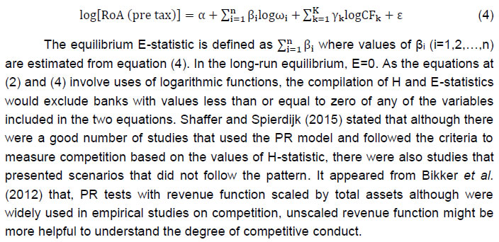

Bikker et al. (2012), however, clarified that uses of unscaled revenue function would require certain additional information, which might not be a straightforward exercise. Bikker and Haaf (2000) used interest revenue (IR) as a dependent variable while Shaffer (1982) and Nathan and Neave (1989) used total revenue (TR) as a dependent variable in their PR models. In view of this, H-statistic for this paper was derived based on two models. The model shown at (5.1) used TR as a dependent variable (referred as PR model 1 in the paper) while the other model shown at (5.2) (to be referred as PR model 2) used IR as a dependent variable.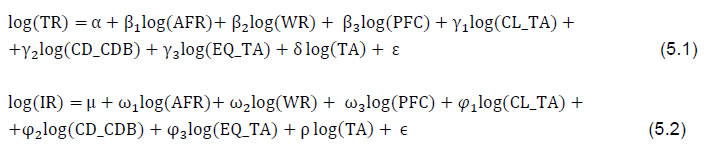

Variables that were used in the equations at (5.1) and (5.2) are defined below. TR was total income, sum of IR and other income. IR was the interest income generated from financial intermediation. AFR, WR and PFC were prices (cost) of input pertaining to fund, labour and fixed capital, respectively. AFR was average funding rate defined as percentage ratio of expenses incurred on payment of interest to total fund (deposits and borrowings), WR was wage rate (per employee cost defined as the ratio of total expenses incurred on employees to total number of employees), PFC (price of fixed capital) was the percentage ratio of other operating expenses (operating expenses excluding expenses on employees) to fixed assets. CL_TA, CD_CDB, EQ_TA and TA were the bank specific control variables. CL_TA was percentage ratio of customer loans (total loans excluding interbank loans) to total assets (TA), CD_CDB was percentage ratio of customer deposits (total deposits excluding interbank deposits) to total of customer deposits and short-term borrowings (borrowings with residual maturity up to one year) and EQ_TA was defined as percentage ratio of capital and reserves & surplus to TA. The behaviour of banks and their risk profile would be reflected through these control variables (Bikker et al., 2012).

The condition of long-run equilibrium was verified using the equation at (4). The operating profit as a percentage of total assets was used as pre-tax RoA. Operating profit is defined as total income (interest and non-interest income) net of total expenses (interest and non-interest expenses). Generalised least squares (GLS) method was used to estimate the equations. GLS method considers information in the unequal variability of the dependent variable across classes and is capable to produce the best linear unbiased estimator (Gujarati and Sangeetha, 2007). The equations were estimated using banks as fixed effects.

Lerner Index (LI) is a popularly used indicator to measure competition developed based on the concept of market power (World Bank, 2020). LI is different from H-statistics (PR Model) validity of which is dependent on market equilibrium. H-statistics is based on gross revenues and thus can be computed with less statistics than LI. An important advantage of LI is that application of the index is not dependent on market equilibrium (Demirgüç-Kunt and Martínez Pería, 2010; L´eon, 2014). LI is an indicator suitable for measuring market power rather than for competition (L´eon, 2014). Variation between price and marginal cost (MC) of the product of a firm is an indicator of the market power enjoyed by the firm. In a market with perfect competition, price and MC will be identical. Variation between the two is inversely related to the intensity of competition (L´eon, 2014). Higher is the value of LI, lower would be the competition. Values of LI lie in the range from 0 to 1. The divergence decreases with an increase in the intensity of competition and increases with a decrease in competition. It is computed based on the following formula that measures the level, by which price exceeds MC.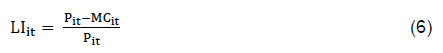

where, LI_it is the value of LI of bank i at time t, P_it and MC_it are, respectively, the price and MC of output of bank i at time t. P_it is taken as the ratio of revenue of bank i to its total assets at time t. MC for a bank at time t is computed from the derivative of a translog cost function as shown below following Demirgüç-Kunt and Martínez Pería (2010):

Variables used in the equation at (7) are defined below. C_it and Q_it, respectively, are the total costs and output of bank i at time t. W_kit is the price of k_th input of bank i at time t. The variable Trend accounts for the impact of technical changes over the period. Total expenses (TE) (interest and non-interest) and total assets of a bank i at time t are used for C_it and Q_it, respectively. u_it is a random error. The MC is then compiled based on the equation shown at (8).

Values of LI in this paper were estimated using the method stated above. GLS method was used to estimate the equation at (7) using banks as fixed effects. AFR, WR and PFC (defined earlier) of bank i for year t were used for W_1it, W_2it and W_3it, respectively.

III.3. Measurement of Stability

Z-score is popularly used to measure stability at an individual bank level. Z-score of a bank is defined as follows (OECD, 2010).

where, sd(RoA) is the standard deviation of RoA of a bank. Profit after tax as percentage to total assets is used for RoA. Higher Z-score implies lower risk and hence higher stability. It is also inferred as accounting-based distance to default measure (Li et al., 2017). A three-year rolling time window is used to calculate standard deviations of RoA allowing time variation (Beck et al., 2013; Cuestas et al., 2017; Kanga et al., 2020). This paper also followed a similar approach to compute sd(RoA) to derive bank-wise values of Z-scores using the formula at (9).

III.4. Models used for derivation of relationships between market share and soundness, market power and soundness of a bank and threshold values for its market share and market power

The relationship between market share and soundness in this paper was examined based on bank-wise values of market shares (in total assets) and Z-scores. Bank wise values of LI and Z-scores were used to investigate the relationship between market power (alternatively lack or low level of competition) and soundness. Higher values of LI indicate lower competition as stated earlier. This paper followed the theoretical stipulations by Martinez-Miera and Repullo (2010) to investigate the relationships. Martinez-Miera and Repullo (2010) model regressed Z-score on the linear and quadratic terms of a measure of concentration or of market power (e.g. LI). It recommended a non-linear relationship of inverse U-shape if the coefficient of level (the linear term) is positive and that of the quadratic term is negative. Lind and Mehlum (2010), however, argued in their paper that quadratic approximation could generate a threshold inaccurately, and hence, a U shape in a situation where the relationship actually was convex but monotone. They also suggested a test to find U shape relationship in their paper. As Martinez-Miera and Repullo (2010) model is popularly used to investigate U shaped relationships, this paper also used this theoretical model as shown in equation (10) (Berger et al., 2008).

where Z_it represents the Z-score of bank i in period t. Market structure is proxied by the market share or LI of bank i in period t. The variables Business Environment_kt (k=1,2, …,n) are used to represent the macro-economic situation in period t. The threshold, also termed as a turning point, for market share or market power is derived using the formula at (11) (Jiang et al., 2008; Berger et al., 2008; Cuestas et al., 2017):

where β₁ and β₂, respectively are the coefficients of linear and quadratic terms in the equation at (10). Market share or market power beyond the threshold may have an unfavourable impact on the stability of the banking system (Cuestas et al., 2017). Principles commonly used in empirical literature to conclude inverse U-shaped relationship are the following - estimated values of the coefficients should be significant statistically and the derived threshold value should fall inside the data range (Lind and Mehlum, 2010; Cuestas et al., 2017).

III.4.1. Model used for derivation of relationships between market share and soundness

The relationship between market share and soundness of a bank in the banking system in India in this paper was examined based on the equation at (12).

The equation at (12) was derived from the equation at (10) with the following modifications. A dummy variable and one year lag of the dependent variable were included among the explanatory variables. Definitions of the variables used in the equation at (12) were as follows. Z_it was the Z-score of bank i in year t, MS_it was the market share of bank i in year t defined as a percentage share of assets of bank i in total assets of the banking system in year t.

Amalgamation_it was a dummy variable used in the model to control for amalgamation. Quite a few amalgamations/mergers of banks took place during the period under reference (Table A1 in the annex furnishes the list of amalgamations during the period under study). Amalgamation_it was assigned value 1 for bank i for year t if bank i amalgamated any other bank into it in year t, otherwise, it was assigned the value 0. The variable ‘real GDP growth_t’ was the annual growth in GDP (at constant prices) of India in year t and was used to represent the business environment. Growth in GDP at constant prices defines real rate of growth in GDP and indicates variations in economic development.

Financial soundness/stability of a bank in the past may impact its soundness/ stability in future. Accordingly, one year lagged value of Z-score was also used as an explanatory variable. ɛit was the random error term. Threshold value for the market share of a bank was derived using the formula given at (11).

Generalised method of moments (GMM) was used to estimate the equations at (12). For a dynamic panel data model, a general approach is to employ GMM to take care of the endogeneity problem (Greene, 2002). The author would like to clarify that there are various statistical software that facilitate the use of GMM employing various specifications for transformation, instrument variables, lags etc. The software and specifications used for GMM estimations in the paper are stated below². The paper used dynamic panel wizard (DPW) in EViews 11 software for estimating the equations. DPW facilitates the use of dynamic panel data methods to develop models that deploy lagged endogenous variables, cross-section fixed effects and multiple lags etc. (IHS Markit, 2019). There is a likelihood of serial correlation of first-order in dynamic panel (Canarella and M. Miller, 2017). Arellano and Bond (1991) first difference method was used to test for serial correlation of first and second order. The corresponding test statistics for first and second order follow normal distribution under the null hypothesis of no first order autocorrelation and no second-order autocorrelation, respectively (Canarella and M. Miller, 2017).

This paper applied the two step GMM approach using transformations based on forward orthogonal deviations (FOD) proposed by Arellano and Bover (1995). Variables that are endogenous in nature, not normal and suffer from unnoticed heterogeneity, can also be used in two step GMM approach (Canarella and M. Miller, 2017). FOD transformations were used following Hayakawa (2009). First lags of the variables on market structure and multiple lags of the dependent variable were used as instrumental variables for GMM³. This means that the model may be over-identified. J statistic (Sargan test) was used to test the null hypothesis that over-identification was valid. Results derived based on GMM were also validated using GLS method.

Equations were estimated using banks as fixed effects for GLS as Hausman test rejected random effect model. It would be worthwhile here to mention an important characteristic of the banking sector in the country. The sector is highly skewed in terms of the sizes (total assets) of banks (Chart 1). In the banking sector in India, over 16 per cent of its total assets were held by SBI during the period covered in the study. Sizes of all other banks in terms of their individual shares in total assets were less than 10 per cent during the same period. In view of such skewed distribution, the relationship between the market share and soundness in the sector was examined with and then without SBI in the sample.

III.4.2. Model used for derivation of relationship between market power and soundness

The equation at (13) was used to examine the relationship between market power and soundness. It was derived from the equation at (12) by replacing bank wise values of market share by bank wise values of LI, used as proxies for market power.

where, LI_it is the value of LI for bank i in year t, all other variables were as defined for the equation at (12). Threshold value for the market power of a bank was derived in terms of LI using the formula given at (11). The equation at (13) was estimated using the same approach followed to estimate the equation at (12) stated in detail above.

IV. Data

The paper used data on annual accounts of SCBs, excluding RRBs, during the period from 1994-95 to 2019-20. All these banks (henceforth referred to as banking system in India) accounted for around 88 per cent of the total assets of the banking sector in the country that comprised of all SCBs, local area banks, non-scheduled payments banks, urban co-operative banks and rural co-operatives at end-March 2020. Banks amalgamated/merged were taken as separate entities until the point of amalgamation/merger. For the compilation of HHI in the paper, all these banks were considered.

It was felt that it would be appropriate to consider only those banks that were in operation in the system at least for a few years to study the level of competition (as it involved examination of long-term equilibrium) and to study the relationships of the market share/ power with soundness. Accordingly, banks that were in operation only for a short period and banks that were licensed in recent years were excluded for assessment of competition and soundness. Banks that were, thus, considered for the PR models and to examine the relationships between market share/ power and soundness were found to be in operation at least for seven years during the period under reference. All these banks accounted for at least 98 per cent of the total assets of all SCBs (excluding RRBs) during the period under study. Data were taken from the publication titled ‘Statistical Tables Relating to Banks in India’ (STRBI) maintained in the RBI website [(RBI, 2020a) and (RBI, 2020b)].

V. Results and Discussion

Values of HHI, H-statistic, market share, LI and Z-scores were compiled for the period under study based on the methodologies and data described in Sections III and IV, respectively. HHI and H-statistic were compiled to assess the level of concentration and competition at a system level. Values of market share, LI and Z-score were compiled at individual bank level to examine the relationships between market share/ power and soundness.

V.1. Level of concentration - values of HHI

Estimated values of HHI for deposits, loans and assets remained between 0.05 and 0.08 for the banking system in India during the period under study (Table A2 in annex). HHI did not change much despite a number of consolidations during the period of study, suggesting a high level of fragmentation and diffusion in the banking sector of the country (Gandhi, 2016). It, thus, may be argued that the banking sector in India was characterised by a low level of concentration during the period under study following the definition on classification of market concentration presented in Table 1 above.

V.2. Level of competition – values of H-statistic

Estimated values of H-statistic for the banking system in India are presented in Table 2. Values of the H-statistic were found between 0 and 1. Wald test rejected the hypotheses of perfect competition (H=1) and that of monopoly (H=0). The equilibrium test failed to reject the null hypothesis E=0, indicating long term equilibrium in the market. The results thus suggested monopolistic competition of the banking system in India during the period under reference.

Estimated values of the coefficients of the variables of the PR models used are presented in Table 3. Regarding the signs of the input prices, Bikker et al. (2012) stated that it would depend on the competitive environment. Bikker and Haaf (2000) found the coefficient of the variables AFR and WR as significant and mostly positive in their PR model applied to 23 countries that used interest income as dependent variable. Signs of the coefficients of these two variables were found as positive in this paper also. They were found significant at 1 per cent level for the PR model 1. For the PR model 2, coefficient of AFR was found significant at 1 per cent level while that of WR was found not significant. Regarding the coefficient of the variable PFC, Bikker and Haaf (2000) found it to differ in size, sign and level of significance across countries and also stated that this variable was probably the least important part of H-statistic.

This paper found the values of the coefficients of this variable to be negligible and not significant for both models. Regarding the sign of the coefficient of the variable CL_TA, this paper found it as positive for both the models as expected in Bikker et al. (2012). Coefficients of the variable were significant at 1 per cent level for both the models. For the variable CD_CDB, Bikker et al. (2012) stated that the exact impact of this variable on interest income was not clear. This paper found a positive impact of CD_CDB on TR and IR, significant at the10 per cent level for both models. Regarding the variable EQ_TA, the signs of its coefficients were found negative for both models. This was in line with the findings in Bikker et al. (2012). Values of the coefficients were, however, not significant for both models. The coefficients of TA were found positive and significant at 1 per cent level for both models.

V.3. Relationship between market share and soundness and estimation of threshold for market share of a bank in the banking system in India

The relationship between market share and soundness in the banking system in India was examined based on bank-wise values of market share in total assets and bank-wise values of Z-score. The relationship was examined applying the model at (12) using GMM, with SBI (the largest Indian bank) as well as without SBI in the sample as explained in detail in section III. The Arellano-Bond test for AR(1) in the first differences showed the presence of serial correlation of first order (p values < 0.05, for both the samples, including SBI and excluding SBI) but the test for AR(2) revealed no presence of serial correlation of second order (p value was 0.73 for the sample including SBI and 0.71 when the sample excluded SBI).

Estimated values of the coefficients derived using GMM (FOD) are presented in Table 4. When the sampled banks included SBI, the estimated value of the coefficient of the linear term of market share was found positive and that of its quadratic term was found negative, both significant at 1 per cent level. P values of J-statistics confirmed that the instruments used for estimation were valid. To validate the results, relationship was also examined applying the model at (12) using GLS as explained in Section III.

Findings were similar to those derived under GMM stated above. It was, however, observed from the results (GMM and GLS) that, absolute values of the coefficients of the quadratic terms of market share were very small in size and also much smaller as compared to absolute values of the coefficients of its linear term. It may, therefore, be suggested as per the model used in this paper that the relationship between market shares and soundness for the banking system in India was possibly non-linear during the period under study. The threshold for market share for a bank in total assets was found at around 19 per cent under GMM (around 14 per cent under GLS). Values of the threshold were inside the data range of bank wise values of market shares observed during the period under study. Market share of a bank in the country in total assets of banking sector beyond the level of 19 per cent may have a negative impact on its soundness/stability.

When the relationship was examined excluding SBI from the sample, estimated value of the coefficient of the linear term of market share was found positive and significant at 5 per cent level and that of the coefficient of its quadratic term also was found positive but not significant under GMM. Under GLS, estimated value of the coefficient of the quadratic term was also found positive and significant at 5 per cent level, but that of the coefficient of the quadratic term was found negative but not significant. GMM results, thus, encourage consolidation among banks sans SBI. The paper, therefore, would like to suggest that consolidation without SBI is desirable. In respect of control variables, coefficient of the variable ‘amalgamation’ was found positive but not significant under GMM as well as under GLS for both the samples considered as mentioned above. Coefficient of the variable ‘annual real growth in GDP’ was also found positive, but significant only under GMM at 10 per cent for the sample including SBI. Coefficient of ‘one year lagged value of Z-score’ was found positive and significant at 1 per cent level under GMM as well as under GLS for both the samples referred above. Positive values of the coefficients of the control variables suggest their favourable impact on soundness/ stability.

Amalgamation of PSBs implemented by GoI after April 2017 involved banks other than SBI. Market share of SBI in total assets already exceeded the threshold value of 19 per cent while shares of all other banks individually in total assets were much lower than the threshold⁴. Share of BoB that amalgamated two PSBs into it in April 2019, increased from slightly above 4.5 per cent as at end-March 2019 to slightly below 6.5 per cent in March 2020. As mentioned earlier, PNB, UBI, Canara Bank and Indian Bank also amalgamated a few other PSBs in April 2020. Shares of each of these banks in total assets of the banking sector in the country, taking into account also the assets of the respective bank(s) each of them amalgamated, were found at around 3 to 7 per cent as per end-March 2020 data. The shares were much below the threshold value derived in the paper.

Results found in the paper as discussed above, thus, suggested that it was a prudent decision by GoI to exercise consolidation of PSBs after April 2017 excluding SBI. The paper would, however, like to suggest that it may also be appropriate to implement the consolidation policy keeping in view the threshold value for the market share of a bank found in the paper so that a bank post amalgamation does not face stability issues.

V.4. Relationship between market power and soundness and estimation of threshold for market power of a bank in the banking system in India

The relationship between market power (alternatively lack or low level of competition) and soundness in the banking system in India was examined based on the relationship between bank wise values of LI and Z-scores. Bank-wise values of LI were estimated using the method presented in Section III. Results of the translog cost function are presented in Table A3 in annex. The relationship between market power and soundness was then examined using the model at (13) in a similar manner followed to examine the relationship between the bank’s market share and its soundness explained above. Arellano-Bond test for AR(1) showed the presence of serial correlation of first order (p values < 0.05, for both the samples, including SBI and excluding SBI) and the test for AR(2) revealed an absence of serial correlation of second order (p values were 0.86 and 0.48, respectively, for the samples including SBI and excluding SBI).

Table 5 presents the estimated values of the coefficients derived using GMM (FOD). Values of the coefficients of the linear terms of LI were found positive and that of its quadratic terms were found negative under all the scenarios (sampled banks including and excluding SBI). Values of the coefficients of the linear terms of LI were found significant at 1 per cent level under GMM as well as under GLS. For the quadratic terms, values of the coefficients were found significant at 1 per cent level for the sample including SBI and at 5 per cent level for the sample excluding SBI under GMM. Coefficients were found significant at 1 per cent level for both the samples under GLS.

Moreover, absolute values of the coefficients of the quadratic terms of LI were not small in size and also not much different from that of its linear terms unlike the results found above in examination of the relationship between market share and soundness. P values of J-statistics confirmed the validity of the instruments used for estimation. The findings thus indicated an inverted U-shaped relationship between bank-wise values of LI and Z-scores and hence between market power (lack or low level of competition) and soundness for a bank in India during the period under study as per Martinez-Miera and Repullo (2010) model.

Threshold values for market power in terms of LI were found at 0.60 under GMM (0.57 under GLS). Values were inside the data range of estimated values of LI during the period under reference. Market power of a bank in the banking system in the country beyond the threshold may impinge upon its soundness. Ninety-five per cent of the banks had their LI values below 0.60 at end-March 2020. Most of the banks with LI values above 0.60 were small in size and with negligible shares in total assets as at end-March 2020. In respect of control variables, observations were almost similar to that found in the study of the relationship between market share and soundness discussed above. The findings above thus suggest that both the views viz., competition-stability and competition-fragility could probably be applicable for a bank in the banking sector in India depending on the level of market power (competition). Both these views probably exist in the banking system in India at different sides of the threshold. There is no clear evidence in the existing literature in favour of either view for the Indian banking system as shown in the paper.

VI. Conclusion

The findings from the paper suggested that the Indian banking system did not have a high degree of concentration, and it broadly suggested a monopolistic competitive structure during the period under study.

The paper found an inverted U-shaped relationship between the market power of a bank and its soundness. Non-linear relationship was also found between the market share of a bank and its soundness during the study period underlining an optimal threshold level of market share for a given bank. The threshold level of market share estimated in the paper can be taken as a guide for any future attempts at consolidation. The findings from the paper supported the recent attempts at consolidation among public sector banks.

While the paper provided broad evidence in support of the strategy of bank consolidation based on its estimated threshold, it did not examine each individual attempt of consolidation in detail. Further research may be necessary to judge whether or not a given attempt of consolidation has been successful depending on the pre-consolidation synergies and post-consolidation performance of the merged entity.

^@ Pradip Bhuyan (pbhuyan@rbi.org.in) is Director in the Department of Currency Management, Reserve Bank of India (RBI).

¹ The author gratefully acknowledges the comments received from an anonymous reviewer, and Radheshyam Verma, Assistant Adviser, Department of Economic and Policy Research (DEPR), who discussed the paper and offered his comments in DEPR Study Circle Seminar. The author is also thankful for the suggestions received in an earlier version of the paper presented in the Department of Statistics & Information Management, RBI. The author sincerely thanks Dr. Pallavi Chavan, Director and her team in Development Research Group, DEPR for their valuable suggestions. The views expressed in the paper are those of the author and do not necessarily reflect the views of RBI.

² Author tried various specifications while applying GMM and presented results of those specifications in the paper that he found more useful.

³ Author could not find good results using single lag of dependent variable as instrumental variable.

⁴ SBI along with ICICI Bank and HDFC Bank are designated as Domestic Systemically Important Banks (D-SIBs) at present (RBI, 2021). All these three banks are therefore subjected to additional Common Equity Tier 1 (CET1) requirement. The additional CET1 requirement is the highest for SBI at 0.60 per cent of risk weighted assets (RWAs); it is 0.20 per cent of RWAs for the other two D-SIBs (RBI, 2021).

⁵ data for the period from 1994-95 to 2003-04 were taken from this source.

References

Allen, F. and Gale, D. (2000a). Financial contagion, Journal of Political Economy 108: 1-33.

Allen, F. and Gale, D. (2000b). Comparing financial systems. Cambridge, MA: MIT Press.

Allen, F. and Gale, D. (2004). Competition and financial stability. Journal of Money, Credit and Banking, 36:3 Pt.2: 433-80.

Ansari, J (2013). A new measure of competition in Indian loan markets, International Journal of Finance & Banking Studies, 2(4): 60-77.

Anzoategui, D., Soledad, M., Pería, M. and Rocha, R. (2010). Bank competition in the Middle East and Northern Africa Region, Policy Research Working Paper 5363, World Bank.

Arellano, M. and Bond, S. (1991). Some tests of specification for panel data: Monte Carlo evidence and an application to employment equations. The Review of Economic Studies.

Arellano, M. and Bover, O. (1995). Another look at the instrumental variable estimation of error components models. Journal of Econometrics.

Arrawatia, R., Misra, A., Dawar, V. and Maitra, D. (2019): Bank competition in India: some new evidence using risk-adjusted Lerner Index approach.

Beck, T., Demirgüç-Kunt, A. and Levin, R. (2005). Bank concentration and fragility: impact and mechanics, Working Paper 11500, National Bureau of Economic Research, June, https://www.nber.org/papers/w11500 accessed on June 15, 2020.

Beck, T., Demirgüç-Kunt, A. and Levine, R. (2006a). Bank concentration, competition, and crises: first results, Journal of Banking and Finance 30: 1581-1603.

Beck, T., Demirgüç-Kunt, A. and Levine, R. (2006b). Bank concentration and instability: impact and mechanics, in: Carey, M., Stulz, R. (Eds.), The Risks of Financial Institutions, Chicago, University of Chicago Press.

Beck, T. (2008). Bank competition and financial stability: friends or foes? https://siteresources.worldbank.org/INTFR/Resources/BeckBankCompetitionandFinancialStability.pdf accessed on June 15, 2020.

Beck, T., Jonghe, O. D., and Schepens, G. (2013). Bank competition and stability: cross-country heterogeneity. Journal of Financial Intermediation, 22(2):218–244.

Berger, A. N., Leora, F. K. and Rima, T. (2008). Bank competition and financial stability, The World Bank, Development Research Group, Finance and Private Sector Team, https://www.researchgate.net accessed on June 15, 2020.

Bhattacharya, K. and Das A. (2003). Dynamics of market structure and competitiveness of the banking sector in India and its impact on output and prices of banking services, Reserve Bank of India Occasional Papers Vol. 24, No. 3, Winter 2003.

Bikker J., and Haaf, K. (2000). Competition, concentration and their relationship: an empirical analysis of the banking industry, Research Series Supervision no. 30, De Nederlandsche Bank, https://www.dnb.nl/en/binaries/ot030_tcm47-146046.pdf.

Bikker, J., Shaffer, S. and Spierdijk, L. (2012). Assessing competition with the Panzar-Rosse model: the role of scale, costs and equilibrium, The Review of Economics and Statistics, 94(4): 1025-1044.

Bishnoi, T. R. and Devi, S. (2017). Banking reforms in India - consolidation, restructuring and performance, Cham: Palgrave Macmillan.

BIS (2001). The banking industry in the emerging market economies: competition, consolidation, and systemic stability, BIS Papers No 4, August; Bank for International Settlements; https://www.bis.org.

Boot, A.W.A. and Thakor, A. (2000). Can relationship lending survive competition?, Journal of Finance, 55: 679-713.

Boyd, J.H., De Nicoló, G. and Smith, B.D. (2004). Crises in competitive versus monopolistic banking systems, Journal of Money, Credit and Banking 36, 487-506.

Boyd, J.H. and De Nicoló, G. (2005). The theory of bank risk-taking and competition revisited. Journal of Finance, 60: 1329-343.

Boyd, J.H. and Prescott, E.C. (1986). Financial intermediary-coalitions, Journal of Economic Theory, 38: 211-232.

Calice, Pietro and Leonida, Leone (2018). Concentration in the Banking Sector and Financial Stability, New Evidence, Policy Research Working Paper, World Bank Group.

Canarella, Giorgio and M. Miller, Stephen (2017). The Determinants of Growth in the Information and Communication Technology (ICT) Industry: A Firm-Level Analysis, Department of Economics working paper series, University of Connecticut, https://www.econ.uconn.edu/.

Cetorelli, N., Hirtle, B., Morgan, D., Peristiani, S. and Santos, J. (2007). Trends in financial market concentration and their implications for market stability, Federal Reserve Bank of New York Policy Review, 33-51.

Cuestas, J. C., Lucotte, Y. and Reigl, N. (2017). Banking sector concentration, competition and financial stability: the case of the Baltic countries, Bank of Estonia (Eesti Pank), https://www.eestipank.ee/en/publications/series/working-papers accessed on June 15, 2020.

Das, S. (2019). Indian banking at crossroads: some reflections, speech delivered at the first annual economics conference, Amrut Mody School of Management, Ahmedabad University, https://www.rbi.org.in, November.

Demirgüç-Kunt, A. and Martínez Pería, S. M. (2010). A framework for analyzing competition in the banking sector, The World Bank, Development Research Group, Finance and Private Sector Development Team, December.

Dubovik, A. and Kalara, N. (2018). Can we measure banking sector competition robustly? CPB Discussion Paper, October, CPB Netherlands Bureau for Economic Policy Analysis.

Dutta, N. (2013). Competition in Indian commercial banking sector in the liberalized regime: An empirical evaluation, International Journal of Banking, Risk and Insurance.

Gandhi, R. (2016). Consolidation among public sector banks, speech delivered at the MINT South Banking Enclave, Bangalore, https://www.rbi.org.in, RBI Bulletin, May.

GoI (2017). Cabinet gives in-principle approval for public sector banks to amalgamate through an alternative mechanism, Press Information Bureau, Government of India, https://pib.gov.in/newsite/PrintRelease.aspx?relid=170187 accessed on June 15, 2020.

GoI (2019). Roadmap for PSBs growth and consolidation, Press Information Bureau, Government of India, https://pib.gov.in/newsite/PrintRelease.aspx?relid=191797 accessed on June 15, 2020.

GoI (2020). Cabinet approves mega consolidation in public sector banks with effect from 1.4.2020, Press Information Bureau, Government of India, https://pib.gov.in/PressReleaseIframePage.aspx?PRID=1605147.

Greene, William H. (2002). Econometric analysis, fifth edition.

Group of Ten (2001). Report on consolidation in the financial sector, Bank for International Settlements, January, https://www.bis.org; https://www.imf.org; https://www.bis.org; accessed on June 15, 2020.

Gujarati, D. and Sangeetha, N. (2007). Basic econometrics, fourth edition.

Hayakawa, K. (2009). First Difference or Forward Orthogonal Deviation- Which Transformation Should be Used in Dynamic Panel Data Models?: A Simulation Study'', Economics Bulletin, 29 (3).

IMF (2001). Financial sector consolidation in emerging markets, Chapter V, International Capital Market Report, International Monetary Fund.

IHS Markit (2019). EViews 11 User’s Guide II.

Jiang, Yi., Lin, Tun and Zhuang, Juzhong (2008). Environmental kuznets curves in the people’s republic of china: turning points and regional differences, December, Asian Development Bank, https://www.adb.org accessed on June 15, 2020.

Kanga, D., Murinde, V., Soumaré, I. (2020). Capital, risk and profitability of WAEMU banks: does bank ownership matter, Journal of Banking and Finance, 114.

Keeley, M.C. (1990). Deposit insurance, risk and market power in banking. American Economic Review, 80: 1183-1200.

Kumar, S. and Gulati, R. (2019). Did the global financial crisis alter the competitive conditions in the Indian banking industry?, Applied Economics Letters, 26:10, 857-865; DOI: 10.1080/13504851.2018.1502865.

L´eon, F. (2014). Measuring competition in banking: a critical review of methods, Etudes et Documents 12, Serie Etudes et documents du CERDI.

Li, Z., Liu, S., Meng, F. and Sathye, M. (2019). Competition in the Indian banking sector: a panel data approach; Journal of Risk and Financial Management, https://www.mdpi.com/journal/jrfm, accessed on October 18, 2020.

Li, X., Tripe, D., and Malone, C. (2017). Measuring bank risk: an exploration of z-score, Massey University, Palmerston North, New Zealand.

Lind, J. T. and Mehlum, H. (2010). With or without u? the appropriate test for a u-shaped relationship, Oxford Bulletin of Economics and Statistics, 72(1):109-118.

Martinez-Miera, D. and Repullo, R. (2010). Does competition reduce the risk of bank failure?, Review of Financial Studies, 23(10): 3638–3664.

Méon, P.G. and Weill, L. (2005). Can mergers in Europe help banks hedge against macroeconomic risk?, Applied Financial Economics, 15: 315-326.

Mishkin, F.S. (1999). Financial consolidation: dangers and opportunities, Journal of Banking and Finance, 23: 675-691.

Misra, A.K. (2011). Competition in banking: the Indian experience, International Conference on Economics and Finance Research, IPEDR Vol.4, IACSIT Press, Singapore.

Nathan, A., and Neave, E.H. (1989). Competition and contestability in Canada’s financial system: empirical results, Canadian Journal of Economics 22, 576-594, https://www.jstor.org/stable/pdf/135541.pdf.

OECD (2010). Policy round tables - competition, concentration and stability in the banking sector, Organisation for Economic Co-operation and Development, https://www.oecd.org/regreform/sectors/46040053.pdf accessed on June 15, 2020.

Panzar, J. and Rosse, J. (1982). Structure, conduct, and comparative statistics, Bell Laboratories Economics Discussion Paper.

Panzar, J. and Rosse, J. (1987). Testing for ‘monopoly’ equilibrium, The Journal of Industrial Economics, 35(4): 443-456.

Prasad, A. and Ghosh, S. (2005). Competition in Indian banking, IMF Working Paper, WP/05/141, July; https://www.imf.org accessed on June 15, 2020.

Rakshit B. and Bardhan S. (2019). Bank competition and its determinants: evidence from Indian banking; International Journal of the Economics of Business, 26 (2): 283–313.

RBI (1995). Annual report, Reserve Bank of India, https://www.rbi.org.in.

RBI (2008). Report on currency and finance, Reserve Bank of India, https://www.rbi.org.in.

RBI (2020a). Statistical tables relating to banks in India (for the period from 2004-05 to 2019-20), Database on Indian economy, Reserve Bank of India, www.rbi.org.in.

RBI (2020b)⁵. Statistical tables relating to banks in India, 1979-2009, https://www.rbi.org.in/Scripts/OccasionalPublications.aspx?head=Statistical%20Tables%20Relating%20to%20Banks%20in%20India%201979-2009, Reserve Bank of India.

RBI (2021). RBI releases 2020 list of Domestic Systemically Important Banks (D-SIBs), Reserve Bank of India, https://www.rbi.org.in.

Rosse, J. and Panzar, J. (1977). Chamberlin vs. Robinson: an empirical test for monopoly rents, Bell Laboratories Economic Discussion Paper.

Sarkar, S., and Sensarma, R. (2016). The relationship between competition and risk-taking behaviour of Indian banks, Journal of Financial Economic Policy, 8 (1): 95–119. doi:10.1108/JFEP-05-2015-0030.

Shaffer, S. (1982). A nonstructural test for competition in financial markets, Federal Reserve Bank of Chicago, Proceedings of a Conference on Bank Structure and Competition, 225–243.

Shaffer, S. and Spierdijk, L. (2015). The Panzar–Rosse revenue test and market power in banking, Journal of Banking & Finance, 61.

Sinha, P., Sharma, S. and Ghosh, S. (2015). An empirical analysis of competition in the Indian Banking Sector in dynamic panel framework, https://mpra.ub.uni-muenchen.de/68556/MPRA Paper No. 68556.

Sinha, P. and Sharma, S. (2016). Relationship of financial stability and risk with market structure and competition: evidence from Indian banking sector, https://mpra.ub.uni-muenchen.de/72247/MPRA Paper No. 72247.

Sinha, P. and Sharma, S. (2018). Dynamics of competition in the Indian banking sector; Economic & Political Weekly, LIII (13).

Subbarao, D. (2013). Banking structure in India – looking ahead by looking back, speaking notes at the FICCI-IBA Annual Banking Conference in Mumbai on August 13, 2013, https://www.rbi.org.in.

Talwar, S.P. (1998), The changing dimensions of supervision and regulation, speech delivered in bank economists' conference, https://www.rbi.org.in accessed on June 15, 2020.

Talwar, S. P. (2001). Competition, consolidation and systemic stability in the Indian banking industry. BIS Papers No 4, August, Bank for International Settlements; https://www.bis.org.

Vives, Xavier (2016). Competition and Stability in Banking: The Role of Regulation and Competition Policy, Princeton University Press.

U.S. Department of Justice (2010). Horizontal merger guidelines, U.S. Department of Justice and the Federal Trade Commission, August.

World Bank (2020). Banking competition, World Bank, https://www.worldbank.org, accessed on June 15, 2020.

Annex