Money market plays an important role in the well-functioning of an economy by providing short-term capital to a wide class of financial entities. The article examines the different money market segments in India and analyses the changes witnessed in the Indian money market during January 2016 to March 2021. The constructed dispersion index that reveals the behaviour of cross-sectional rate dispersion in the money markets, indicates a frictionless market with efficient pass-through during the period before the declaration of the pandemic in January 2020-February 2020. The decreasing trend in the dispersion index in the recent times suggests stabilisation of the markets and adaptation to the new normal. Introduction Money market is an integral part of the financial system and includes instruments that provide short-term funds with maturity ranging from overnight to one year. As the short-term money market rates often serve as operational targets of central banks, the money market plays a key role in the transmission of monetary policy. Money market has emerged as the router for the transmission of policy impulses across the financial system and is essential for extracting important information related to the expectations of future movements in interest rates (Bhattacharyya et al., 2009). As the money market rates serve as benchmarks for the pricing of credit, it plays an important role in determining the credit conditions in the economy and in turn the level of lending rates faced by firms and households (Corradin et al., 2020). Money market generally includes short-term unsecured (uncollateralised) interbank loans, secured (collateralised) loans (including repurchase agreements), treasury bills (T-bills), commercial papers (CPs) and certificates of deposit (CDs). Participants in these markets typically include, banks, investment funds and non-financial corporations. A well-functioning interbank market (where banks borrow from and lend to each other) can ensure efficient liquidity transfer between surplus and needy banks (Furfine, 2001; Acharya et al., 2012). During the recent episodes of financial distress induced by the Covid-19 pandemic, money market too came under stress with volatile interest rate spreads and trading activity. In the past, tension in the money market has resulted in banks replacing money market funding with central bank funding globally. Further, central bank interventions conducted in the wake of a financial crisis, are known to impact money markets. For instance, large-scale asset purchases conducted during the Global Financial Crisis (GFC) had a significant impact on money markets. During the GFC and Euro area’s sovereign debt crisis, cross-sectional dispersion in the interbank money market rates raised the lending rates banks charge to firms (Altavilla et al., 2019). Therefore, in addition to studying the changes in volumes, rates and microstructure, money market dispersion (deviation of cross-sectional distribution of money market rates) is also of importance to the central banks as this can indicate market segmentation and provide an understanding of the funding cost of banks. With this background, it would be interesting to examine the different money market segments in India and analyse the changes witnessed in the Indian money market. In India, money markets have gone through substantial changes in the past five years. The volumes and rates in the money market segments have broadly evolved with changing monetary policy stance and banking system liquidity conditions. The period considered for the study — January 2016 to March 2021, provides an opportunity to examine the shifts experienced in the money markets in view of the adoption of the inflation targeting regime, change in the liquidity conditions during November 2016 following the Indian banknote demonetisation, availability of payment systems on a 24x7 basis, adoption of the revised liquidity management framework in February 2020, and the different policy measures (including the unconventional monetary policy measures to provide liquidity in the financial system) undertaken by the Reserve Bank (since end- February 2020) to mitigate the stress induced by the Covid-19 pandemic. The article is structured as follows: Section II provides an overview of the different segments of the Indian money market. Section III presents stylised facts related to money markets, collected from literature and examines the relevance of these theories in the Indian context. Section IV measures dispersion of money market rates using an index termed as the Dispersion Index (proposed by Duffie and Krishnamurthy, 2016), which combines information of money market rates and volumes. This is followed by an analysis to determine the important factors that influence dispersion of money market rates in the Indian setup. Section V provides the concluding observations. II. Salient Features of the Indian Money Market The Reserve Bank undertakes monetary operation under the Liquidity Adjustment Facility (LAF) and manages liquidity in the banking system. For providing short-term funds, the Indian money market includes call money, triparty repo [erstwhile collateralised borrowing and lending obligation (CBLO)1], market repo, repo in corporate bonds, CPs, CDs and T-Bills. The details of these segments are presented in Annex-Table A.1 In India, commercial banks, co-operative banks, primary dealers (PDs), insurance companies, mutual funds (MFs), non-banking financial companies (NBFCs), corporates are permitted to participate in money markets. The share of each money market segment in the overall volume along with the trend in the average daily volume in the money markets is given in Chart 1a. The average volume has increased, with the increase being steeper in the recent times. Further, CBLO/triparty repo dominate in terms of volume with a share of around 58 per cent (during the period from January 2016 to March 2021). The rates in the different money market segments tend to move in tandem and the CP rates generally trade at the highest (Chart 1b). In the call money segment2, the overnight segment dominates in terms of volume. Despite several measures taken by the Reserve Bank, the volume in the term money segment remains very low. However, the share of the term money in the total call money volume increased marginally in 2020-21 and stood at 3.6 per cent in comparison to 2.5 per cent in 2019-20. In the term money segment, trading is mainly concentrated in the tenor of 15-30 days (Chart 1c). Some of the reasons for the general under development of the term segment include: (i) the inability of market participants to build interest rate expectations over the medium term; (ii) the skewed distribution of liquidity; and (iii) the preference of banks for LAF reverse repo operations over term money market to deploy their surplus funds (Patra et al., 2016). Further, market repo may be categorised into two − Basket Repo and Special Repo. Basket repo is the general collateral repo and special repo helps in obtaining a particular security for meeting any delivery obligation against short sale position. Basket repo accounts for the larger market share in comparison to special repo, although volume in the latter has shown a steady increase in the recent years (Chart 1d). As the rate in the special repo segment depends on the availability of a particular security, any short supply can push down the borrowing rates, thus making basket repo a better representative of the money market than special repo (Nath, 2018). III. Stylised Facts This section presents the important stylised facts related to money markets available in the literature and focus is mainly kept on the behaviour of money markets during times of financial crisis. The relevance of these theories is checked for in the Indian context. Stylised Fact 1: Money markets experience bouts of volatility during financial crisis and increasing the amount of excess reserves lowers overnight rate volatility (Corradin et al., 2020; Bech and Monnet, 2016). A review of volatility is important as lower volatility in the overnight interbank rate would reduce the uncertainty about funding costs (Kavediya and Pattanaik, 2016). The important drivers of volatility of the overnight call money rate (the operating target of monetary policy) are system liquidity and policy repo rate (RBI, 2021). These two factors are bound to undergo changes as a result of the measures taken by the central bank to mitigate the risks arising from uncertainty during a financial crisis. Volatility in the overnight money market (call/notice, CBLO/triparty repo, market repo), measured as the coefficient of variation3 of the volume-weighted rates increased after the declaration of the Covid-19 pandemic (Chart 2). After the volatility peaked in March 2020, it declined subsequently. Stylised Fact 2: During financial crisis, there is a shift away from unsecured markets and towards the secured markets (Corradin et al., 2020). The volume shares of the unsecured segment (call money) and the secured segment (CBLO/triparty repo and market repo) in the overall volume are given in Chart 3a. The increase in the share of secured volume in 2020-21 (from 93 per cent to 97 per cent) and the subsequent decline in the share of unsecured volume validates the shift away from unsecured markets during uncertain times. Further, the decline in the average daily volume in the unsecured money market segment after the declaration of the Covid-19 pandemic is evident in Chart 3b. Stylised Fact 3: Increasing the amount of excess reserves drives the overnight interbank rate towards the floor of an interest rate corridor (Bech and Monnet, 2016). From the plot of surplus liquidity [net LAF outstanding, (+) absorption] and overnight volume-weighted average rates along with the policy corridor, it can be seen that as the magnitude of system liquidity increased, resultant on the proactive measures taken by the Reserve Bank in order to mitigate the risks arising from the Covid-19 pandemic, the rates have dipped below the reverse repo rate (Chart 4a). Further, the scatter plot based on daily observations of surplus liquidity and overnight volume-weighted average rates indicate an inverse relationship (Chart 4b). Stylised Fact 4: Increasing the amount of excess reserves does not impact the recourse to the central bank lending facility (Bech and Monnet, 2016). The causal relationship in the Indian context is explored by considering the utilisation of marginal standing facility (MSF), a window provided by RBI to banks for borrowing in emergency situations, against banking system liquidity. Consideration of a long time period may not be indicative of the relationship due to changes in system liquidity, availability of payment systems for 24x7, discontinuation of the daily conduct of fixed rate repo operations as a part of the adoption of the revised liquidity management framework etc. Interestingly, the correlations between MSF utilisation and system liquidity during the recent period (January 2020-March 2021), when the liquidity was in surplus and a distant period (November 2013-June 2015), when the liquidity was in deficit are (-) 0.511 and (-) 0.510 respectively. Further, three pairs of Granger causality tests conducted for the period from November 2013 to March 2021 on the variables −system liquidity, MSF volume and overnight money market volume suggest that system liquidity causes overnight money market volume, but not MSF volume (Annex-Table A.2). Moreover, overnight money market volume does not impact MSF volume. The utilisation of MSF is therefore independent of the prevalent liquidity conditions. Stylised Fact 5: Financial crisis impact the intraday interest rate causing different average interest rates in the morning session and afternoon session (Baglioni and Monticini, 2013). For this, intraday rates are calculated in the call money, CBLO/triparty repo and market repo segments of the money market. Due to changing liquidity conditions and policy rates, intraday rates are calculated separately for four scenarios that capture the period when the system liquidity was in deficit; period after demonetisation, when the system turned to surplus mode; and the periods before and after the declaration of the Covid-19 pandemic. Also, scenarios are chosen in such a way that within each scenario, the policy repo rate has remained unchanged. Accordingly, the scenarios are: scenario 1: April 2016-June 20164; scenario 2:-November 2016-July 20175; scenario 3: October 2019-February 20206; and scenario 4: May 2020-March 20217. The movement of intraday average trading volume and weighted average rate (WAR) in the four considered scenarios are shown separately for the call money, triparty repo and market repo segments (Charts 5, 6 and 7). 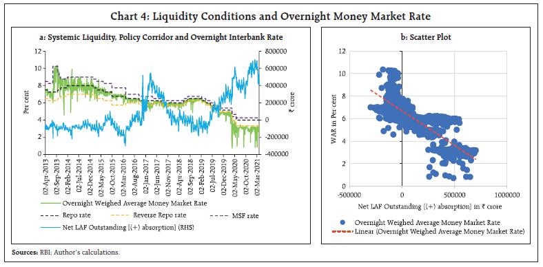 In scenarios 1, 2 and 3, it can be seen that the intraday call money trading is largely concentrated in the first and last hour and has a U-shape. Trading increases in the last hour after the closing of CBLO/ triparty repo and market repo segments. It can be seen that when the system liquidity was in deficit, trading is highest in the first hour (Chart 5a). However, as the system liquidity turned to surplus, trading reduced in the first hour and was highest in the last hour (Charts 5b, 5c). Further, in scenario 4, after adoption of truncated market hours, trading activity is not seen to follow the earlier U-shaped curve (Chart 5d). 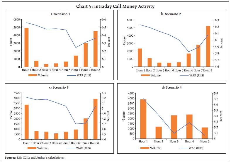 In the case of WAR, it can clearly be seen that in scenarios 1, 2 and 3, rates are the highest in the first hour and witnesses a slump in the sixth hour only to increase later in the last hour. During the first three scenarios, the average difference between the WAR in the first hour and sixth hour range between (-) 31 to (-) 51 bps. In scenario 4, in the period after the declaration of the Covid-19 pandemic, the pattern is different and WAR drops by 61 bps in the third hour and drops further in the last hour after experiencing an increase in the fourth hour. During the period when the system liquidity was in deficit, trading in the CBLO segment was seen to increase towards the end of the day (Chart 6a). This has changed when the system turned to surplus mode with the first hour dominating in terms of trading activity (Charts 6b, 6c and 6d). Unlike the call money segment, the intraday WARs have not undergone major changes in pattern in scenario 4. This could be attributed to the fact that the important participants like MFs and insurance companies in the triparty repo do not maintain current accounts with the Reserve Bank and do not have direct access to the liquidity facilities of the Reserve Bank. However, the steep rises and declines witnessed in the first three scenarios are absent in scenario 4 due to multiple changes in the net asset value (NAV) cut-off timings of MFs for overnight and liquid schemes during 2020-21. 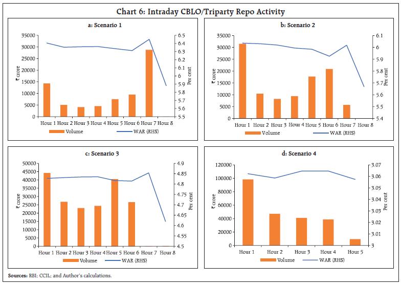
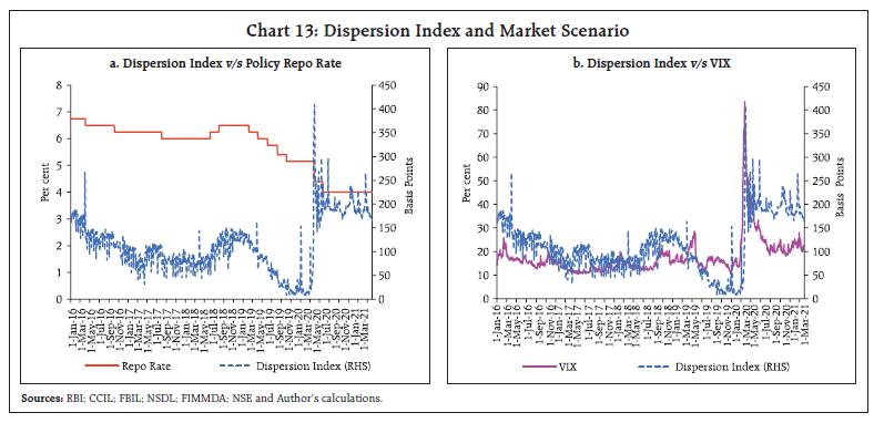
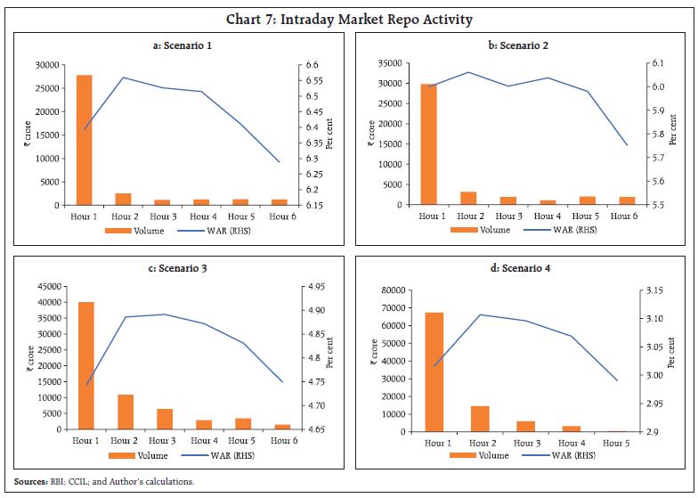 The pattern of increased trading activity in the first hour in the market repo segment followed by a drastic reduction in the subsequent hour has remained unchanged in the considered four scenarios (Charts 7a, 7b, 7c and 7d). Even in the case of WAR, the rates have shown a steady increase in the second hour followed by a drop in the rates in the last hour in all the four scenarios. This constant pattern across all four scenarios in market repo may be due to the inaccessibility of the important market participants to the liquidity facilities of the Reserve Bank, like in the case of triparty repo. Stylised Fact 6: Unconventional Monetary Policy (unprecedented policy measures taken by the central bank that include collateral policies; asset purchase programmes and forward guidance) can significantly change interbank structures (Wolski and van de Leur, 2016). As in the case of the intraday trading activity, the market structure, studied by way of network diagrams, is examined separately for the same four scenarios for the three important money market segments (Charts 8, 9 and 10). Network diagram provides a graphical depiction of the network, with the nodes representing the participants and the link representing the presence of a transaction between the nodes. The graphs prepared are based on the Kamada-Kawai algorithm8. Here, the size of the nodes represents the share of the entity in lending and the links are weighted by the WAR between the nodes. In the call money market, co-operative banks have remained the biggest lender since scenario 2. The network structure which was relatively simple in scenario 1 has become complex in scenario 4 with more interconnections and varying link weights. This suggests that banks have adopted diverse portfolio allocation based on the funding requirements (Chart 8d). In the CBLO/triparty repo segment, MFs followed by insurance companies have dominated as the important lenders in all the four scenarios (Chart 9). On comparing scenarios 1 and 4, it can be seen that interconnections have increased. Although the market has more interconnections in scenario 3 (in the pre-Covid period) in comparison to scenarios 1 and 2, the market structures have not changed significantly from scenario 3 to scenario 4. As the share of lending by banks is nominal in the triparty repo segment, there is reduced impact of liquidity conditions on portfolio diversification. 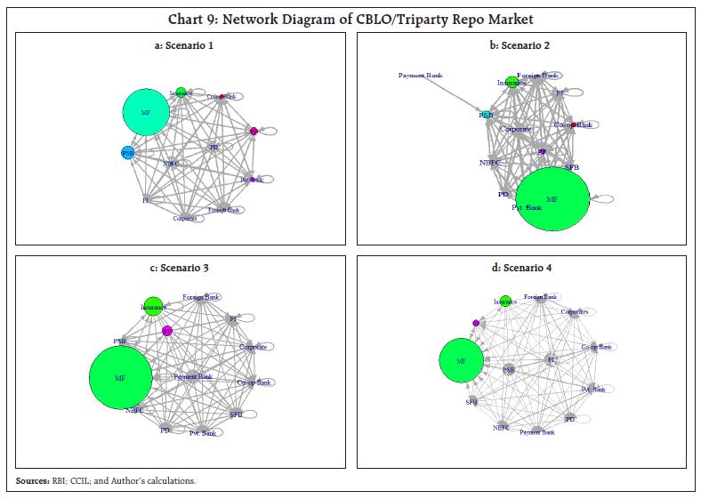 On comparing network diagrams of the market repo segment, it can be seen that public sector banks were displaced by foreign banks as the biggest lender in scenario 2 (Charts 10a and 10b). Foreign banks indulge in short-selling and buy shorter-maturity bonds and trade to make profits. Foreign banks are active on both the borrowing and lending sides in the market repo segment due to the availability of the special repo facility. Further, shares of MFs in lending increased and were dominant in scenarios 3 and 4 (Charts 10c and 10d). The growth of the MF industry has resulted in their increased participation in the market repo segment and the average volume of the overall segment increased from ₹39,669 crore in scenario 1 to ₹85,690 crore in scenario 4. The marginal changes in the interbank connections from scenario 3 to scenario 4 may be attributed to the changes in the composition of special repo facility in the market repo segment (as seen in Chart 1d). 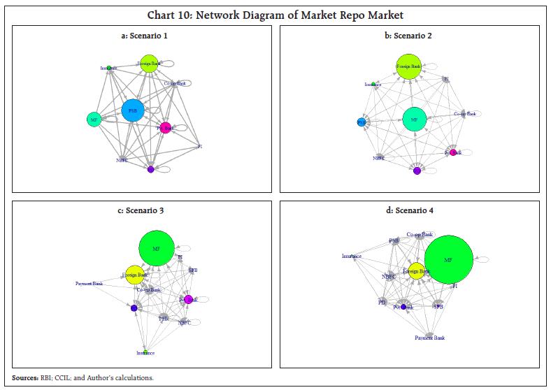 IV. A Dispersion Index for the Indian Money Market Money market activity in secured and unsecured segments is normally measured considering important metrics like volumes, rates and spreads. A dispersion index was designed that explores the behaviour of cross-sectional rate dispersion in the US-dollar money markets (Duffie and Krishnamurthy, 2016). The index is designed in such a way that it would be zero in frictionless market without measurement noise and its actual level would reflect cross-sectional variation in rates caused by pass-through frictions. The dispersion index combines information of money market rates and volumes and is measured as the weighted absolute deviation of the cross-sectional distribution of the overnight rates. Although the constructed index suffers from limitations in terms of availability of data, the dispersion index may serve as an empirical gauge of pass-through efficiency. IV.1 Construction of the Dispersion Index The index construction is based on the methodology outlined in Duffie and Krishnamurthy (2016). However, modifications are made to adapt to the Indian markets. For the construction of the index, daily data on rates and volumes are collected on the different money market segments including call money, CBLO/triparty repo, market repo, CPs, CDs and T-bills for the period from January 01, 2016 to March 31, 20219. Although the focus is on overnight volumes and rates10, due to the non-availability of data for CPs, CDs and T-bills, approximations are made using 3-month rates and overall trading volume. The details are presented in Annex-Table A.3. 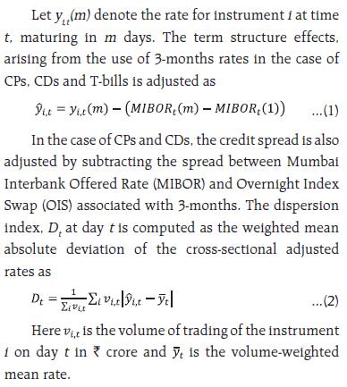 The dispersion index (expressed in basis points) for the considered period is plotted in Chart 11. The index witnessed peaks at the end of every financial year, in end-March, when the money market rates normally increase owing to the demand for funds (due to liquidity management at the end of the annual report disclosure cycle). During the period before the declaration of the pandemic, the dispersion index touched lows in January 2020-February 2020 indicating a frictionless market with efficient pass-through. The onset and declaration of the Covid-19 pandemic caused the dispersion index to peak in March 2020, as extreme risk-aversion gripped investors which resulted in the triparty repo and market repo segments trading at near-zero rate levels. However, dispersion started showing a decreasing trend subsequently, albeit at elevated levels in comparison to the pre-Covid-19 period. Further, towards the end of the period under consideration, the dispersion index started displaying a more prominent decreasing trend suggesting stabilisation of the markets and adaptation to the new system. 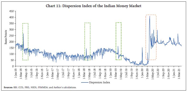 The frequent dips in the index witnessed during the initial period of consideration may be attributed to the effect of Reporting Fridays. As already seen, CBLO is a preferred money market segment with the highest trading volumes on non-Reporting Fridays. The funds borrowed under CBLO qualified for reserve requirements and banks were required to include the CBLO borrowing in their net demand and time liability (NDTL). Further, banks were also required to maintain statutory liquidity ratio (SLR) against the borrowing under CBLO. On the other hand, market repo is exempted from SLR/ Cash Reserve Ratio (CRR) computation. Therefore, the CBLO rates dipped to low levels on Reporting Fridays as liquidity shifted from CBLO to market repo. The rates reverted then to usual levels after the Reporting Friday. However, after triparty repo replaced CBLO in November 2018, this shifting of liquidity to market repo ceased as the borrowing under triparty repo is also exempted from CRR/SLR11. This has resulted in a smoother index since November 2018. This dispersion index is next compared to the banking system liquidity (Chart 12a). From the box plot (Chart 12b), it can be seen that the median of dispersion is higher for the period when the liquidity is in deficit and the distribution of dispersion in the period of surplus liquidity is skewed. It may however be noted that the period under consideration witnessed more episodes of the banking system being in surplus than being in deficit. The dispersion index is then compared with important financial market drivers/indicators — policy repo rate and NSE-Volatility Index (VIX), which indicates stress in the financial markets (Chart 13). The shifts in the mean of the dispersion rate with changes in the policy rate is evident in Chart 13a. The correlation between dispersion index and policy repo rate is significant at (-) 0.38 for the entire sample period considered. However, the correlation is positive and significant at 0.86 for the period from January 2016 to May 2018 (this period witnessed only rate cuts). On considering a similar period that witnessed only rate cuts – from February 2020 to March 2021, the correlation is significant at (-) 0.70. This disparity during the pandemic is further explored by comparing the dispersion index with the prevalent risk appetite in the financial markets, NSE-VIX, which touched record highs after the declaration of the Covid-19 pandemic. Strong co-movement is visible in the patterns of VIX and dispersion index with the correlation between dispersion index and VIX significant at 0.51 for the entire sample period (Chart 13b). 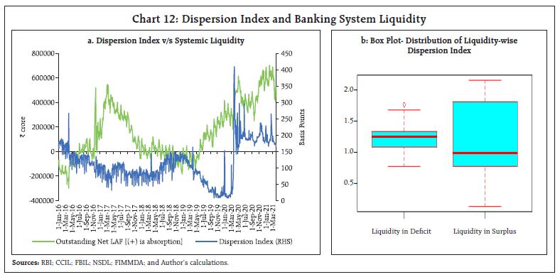
 IV.2 Determinants of the Dispersion Index The determinants of the dispersion index are empirically investigated based on pointers available in literature. Due to the presence of variables of different orders of integration, the model is estimated using the autoregressive distributed lag (ARDL) cointegration procedure (Pesaran et al., 2001). As the results obtained with the use of daily data were not robust due to problems like heteroscedasticity, data is converted to monthly values. The variables considered in the analysis include: (i) average dispersion index (Disp_in); (ii) policy repo rate (Repo); (iii) 1-month realised volatility in SENSEX (Vol); (iv) net liquidity position under LAF12 as a percentage of the banking system’s NDTL (Net_LAF); and (v) net purchase under Open Market Operations (OMO) as a percentage of G-sec market turnover (Net_OMO) and dummies for financial year-end and onset of pandemic. The results of the unit root tests conducted on the variables considered in the analysis are given in Annex-Table A.4. The variables — Net_OMO and Vol are stationary at levels while the other variables are stationary in first difference. A general-to-specific modelling approach guided by Schwartz Bayesian Criterion is used to determine the lag lengths of the ARDL model. The presence of a cointegrating relationship between the dispersion index and the other variables is confirmed by the conduct of Bounds test (Pesaran et al., 2001). The results are provided in Table 1. | Table 1: ARDL Bounds Test Results for Cointegration | | Function | F-statistics | | Disp_in=f(Net_LAF, Net_OMO, Vol, Repo) | 5.82 | | Critical Bounds | 10% | 5% | 1% | | Lower Bounds | 2.2 | 2.56 | 3.29 | | Upper Bounds | 3.09 | 3.49 | 4.37 | | Source: Author’s estimates. | The long-run and short-run estimates of the ARDL model are presented in Table 2. The diagnostic tests indicate absence of serial correlation and heteroscedasticity. The estimated coefficients of the long-run relationship show that system liquidity13 and market uncertainty (measured by SENSEX realised volatility) have a positive and significant impact on the dispersion index. While policy repo rate has a negative and significant impact on dispersion, RBI’s OMO purchases were not found to have an impact on dispersion. From the results of the short-run dynamic coefficients obtained by estimating an error correction model associated with the long-run estimates, it can be seen that RBI’s OMO purchases do not have an impact even in the short run. The signs of the short-run dynamic impacts are maintained in the long-run as well. The dummies for financial year-end and pandemic period have the expected positive and significant coefficients. | Table 2: Results of ARDL(1,1,0,0,2): Long-run and Short-run Estimates | | | Coefficient | P-value | | Long-run estimates | | Net_LAF | 0.0004* | 0.10 | | Net_OMO | 0.0014 | 0.40 | | Vol | 0.0107* | 0.06 | | Repo | -0.1968*** | 0.00 | | Short-run estimates | | ∆Disp_in(-1) | -0.2933*** | 0.01 | | Σ∆Net_LAF(0 to -1) | 0.0009*** | 0.00 | | ∆Net_OMO | 0.0007 | 0.29 | | ∆Vol | 0.0048*** | 0.00 | | Σ∆Repo(0 to -2) | -0.2112** | 0.04 | | ecm(-1) | -0.4436** | 0.04 | | Constant | -0.0251* | 0.05 | | Diagnostics | | Breusch-Godfrey LM test for autocorrelation p-value | 0.2429 | | | LM test for autoregressive conditional heteroscedasticity p-value | 0.3853 | | Source: Author’s estimates. Note: Δ is the difference operator. | The equilibrium correction coefficient [(-) 0.4436] is statistically significant with the expected negative sign and suggests a moderate speed of adjustment to equilibrium after a shock. The cumulative sum (CUSUM) from a recursive estimation of the model also indicate stability in the coefficients (Chart 14). Financial market volatility positively impacts dispersion index in the long-run and short-run which are in expected lines. The positive impact of surplus liquidity may be due to the segmentation between entities that have access to the liquidity facilities extended by the Reserve Bank and those that do not have access. However, as the Reserve Bank started undertaking sector-specific, institution-specific and instrument-specific liquidity measures, dispersion started showing a decreasing trend. Although positive, the OMO purchases undertaken by the Reserve Bank did not impact dispersion. This suggests that there is no collateral scarcity in India which was considered as an important reason for increased dispersion witnessed in the Euro area in the wake of asset purchases by the central bank during the crisis period. (Corradin et al., 202014). Further, the sample period under consideration witnessed multiple trends in OMO operations, with prolonged periods of OMO sales in mid-2017 followed by a period when no operation was undertaken (Annex-Chart A.1). Since December 2019, RBI has undertaken OMO purchases and simultaneous sale and purchase of OMOs. A better understanding of the impact of OMO operations on dispersion would therefore require a separate scenario analysis with more data points that are not currently available. Similarly, the impact of decreasing repo rate on increasing dispersion needs to be further explored for a longer period as the policy rate has undergone more rate cuts in the period under consideration and has fallen from 6.75 per cent in January 2016 to 4 per cent in March 2021. 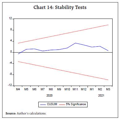 V. Conclusion Money market is an integral part of the financial system and plays a key role in the implementation and transmission of monetary policy. In India, money markets have broadly evolved with changing monetary policy stance and banking system liquidity conditions. The different segments of the money markets were analysed in terms of volume, rates, microstructure and dispersion during the period from January 2016 to March 2021, with a special focus on the period after the onset of Covid-19 pandemic. The article showed an increase in overnight money market volatility after the declaration of the Covid-19 pandemic that peaked in March 2020 and a shift away from unsecured markets and towards the secured markets. Further, the intraday market activity and network structure have undergone changes after the onset of the pandemic with the changes being more prominent in the call money market. The constructed dispersion index that reveals the behaviour of cross-sectional rate dispersion in the money markets, indicated a frictionless market with efficient pass-through during the period before the declaration of the pandemic in January 2020-February 2020. Market uncertainty was found to be associated with increasing money market dispersion. The impact of decreasing repo rate on increasing dispersion needs to be further explored for a longer period as the policy rate has undergone more rate cuts in the period under consideration and has fallen from 6.75 per cent in January 2016 to 4 per cent in March 2021. Although the impact of surplus liquidity on money market dispersion was found to be positive, the sector-specific, institution-specific and instrument-specific liquidity measures undertaken by the Reserve Bank have resulted in a decreasing trend in the dispersion index in the recent times. This suggest stabilisation of the money market with the market adapting to the new normal. References Acharya, V. V., Gromb, D., & Yorulmazer, T. (2012). Imperfect competition in the interbank market for liquidity as a rationale for central banking. American Economic Journal: Macroeconomics, 4(2), 184-217. Altavilla, C., Brugnolini, L., Gürkaynak, R. S., Motto, R., & Ragusa, G. (2019). Measuring euro area monetary policy. Journal of Monetary Economics, 108, 162-179. Baglioni, A., & Monticini, A. (2013). Why does the interest rate decline over the day? evidence from the liquidity crisis. Journal of Financial Services Research, 44(2), 175-186. Bech, M., & Monnet, C. (2016). A search-based model of the interbank money market and monetary policy implementation. Journal of Economic Theory, 164, 32-67. Bhattacharyya, I., Roy, M., Joshi, H., & Patra, M. D. (2009). Money market microstructure and monetary policy: the Indian experience. Macroeconomics and Finance in Emerging Market Economies, 2(1), 59-77. Corradin, S., Eisenschmidt, J., Hoerova, M., Linzert, T., Schepens, G., & Sigaux, J. D. (2020). Money markets, central bank balance sheet and regulation (No. 2483). ECB Working Paper. Duffie, D., & Krishnamurthy, A. (2016). Passthrough efficiency in the fed’s new monetary policy setting. In Designing Resilient Monetary Policy Frameworks for the Future. Federal Reserve Bank of Kansas City, Jackson Hole Symposium (pp. 1815-1847). Furfine, C. H. (2001). Banks as monitors of other banks: Evidence from the overnight federal funds market. The Journal of Business, 74(1), 33-57. Kavediya, R., & Pattanaik, S. (2016). Operating Target Volatility: Its Implications for Monetary Policy Transmission. RBI Occasional Papers, 37(1), 63-85. Nath, G.C. (2018). Repo market and market repo rate as a collateralized benchmark rate. In CCIL Monthly Newsletter-August 2018. Patra, M. D., Kapur, M., Kavediya, R., & Lokare, S. M. (2016). Liquidity Management and Monetary policy: From corridor play to marksmanship. In Monetary Policy in India (pp. 257-296). Springer, New Delhi. Pesaran, M. H., Shin, Y., & Smith, R. J. (2001). Bounds testing approaches to the analysis of level relationships. Journal of applied econometrics, 16(3), 289-326. RBI (2021). Report on Currency and Finance (RCF) 2020-21. February 2021. Wolski, M., & van de Leur, M. (2016). Interbank loans, collateral and modern monetary policy. Journal of Economic Dynamics and Control, 73, 388-416
Annex | Annex-Table A.1: Money Market Timings | | Segment | Type | Reporting Platform | Eligible Participants/Issuers | Market Timings | Revised Existing Timings | | Call Money | Purely unsecured interbank market | NDS-CALL | Scheduled Commercial Banks (including Small Finance Banks), Payment Banks and Regional Rural Banks (RRBs), Co-operative Banks and PDs | 9:00 AM to 5:00 PM | 10:00 AM to 3:30 PM | | CBLO/Triparty Repo | Collateralised borrowing/ lending with the eligible collateral as central government securities and T-bills | Triparty Repo (Dealing) System (TREPS) | Commercial banks, co- operative banks, PDs, financial institutions, insurance companies, mutual funds, NBFCs, corporates and provident/pension funds etc. | 9:00 AM to 3:00 PM* | 10:00 AM to 3:00 PM | | Market Repo | Collateralised borrowing/ lending undertaken among the market participants, with CCIL providing guarantee of settlement of all deals | Clearcorp Repo Order Matching System (CROMS) | Commercial banks, co- operative banks, PDs, financial institutions, insurance companies, mutual funds, NBFCs, listed and unlisted companies, subject to certain conditions | 9:00 AM to 2:30 PM** | 10:00 AM to 2:30 PM | | Repo in Corporate Bond | Repos collateralised by corporate bonds to manage liquidity and asset-liability mismatches | CCIL-Financial Market Trade Reporting and Confirmation Platform (F-TRAC) | Scheduled commercial banks [excluding RRBs and Local Area Banks (LABs)], PDs, NBFCs, All India Financial Institutions (AlFIs), MFs, Housing Finance Companies (HFCs), and insurance companies | 9:00 AM to 6:00 PM | 10:00 AM to 3:30 PM | | Commercial Papers (CPs) | Unsecured money market instrument issued in the form of a promissory note by corporate borrowers | F-TRAC | Companies and AIFIs (subject to the conditions laid out by RBI and SEBI) | 9:00 AM to 5:00 PM | 10:00 AM to 3:30 PM | | Certificates of Deposit (CDs) | Negotiable money market instrument with minimum amount of ₹ 1 lakh and the maturity not less than 7 days and not more than a year15 | F-TRAC | Scheduled commercial banks (excluding RRBs and LABs) and select AlFIs | 9:00 AM to 5:00 PM | 10:00 AM to 3:30 PM | | Treasury Bills | Short-term debt instruments issued by the Government of India | NDS-OM | Government of India. Commercial banks (including Bank-PDs) hold the major share in ownership of T-bills (Annex-Chart A.2) | 9:00 AM to 5:00 PM*** | 10:00 AM to 3:30 PM | Notes: In order to minimise the risks from Covid-19, the trading hours were revised in 2020.
* The timings for the entities settling through Designated Settlement Banks (DSB) is from 9:00 AM to 2:30 PM and the timings for the settlement on T+1 basis is from 9:00 AM to 5:00 PM.
** The timings for the settlement on T+1 basis is from 9:00 AM to 5:00 PM.
*** The timings for the settlement on T+0 basis is from 9:00 AM to 2:30 PM.
Sources: RBI; RBI (2021); CCIL. |
| Annex-Table A.2: Pairwise Granger Causality Tests | | Null Hypothesis | P-value | | System liquidity does not cause MSF volume | 0.1721 | | MSF volume does not cause system liquidity | 0.9438 | | Surplus liquidity does not cause overnight money market volume | 0.0050 | | Overnight money market volume does not cause surplus liquidity | 0.3057 | | Overnight money market volume does not cause MSF volume | 0.5608 | | MSF volume does not cause overnight money market volume | 0.4129 |
| Annex-Table A.3: Details of Main Components of Dispersion Index | | S.No. | Market Segment | Data Used for Rate and Volume | Sources | | 1. | Call Money | Rate and volume of call/notice segments | RBI; CCIL | | 2. | CBLO/Triparty Repo | Rate and volume of overnight and term segments | RBI; CCIL | | 3. | Market Repo | Rate and volume of overnight and term segments | RBI; CCIL | | 4. | Commercial Paper | 3-month rate and overall issuance in primary market | FIMMDA; CCIL; NSDL; Author’s calculations | | 5. | Certificate of Deposit | 3-month rate and overall issuance in primary market | FIMMDA; CCIL; NSDL; Author’s calculations | | 6. | T-bill | 91-day rates and overall trading volume in secondary market | CCIL; FBIL |
| Annex-Table A.4: Results of the Unit Root Tests | | Variable | Augmented Dickey Fuller Test Statistic | Phillips-Perron Test Statistic | | Disp_in | -2.13 | -1.96 | | ∆( Disp_in) | -5.74*** | -5.72*** | | Net_LAF | -1.75 | -1.51 | | ∆( Net_LAF) | -6.37*** | -6.40*** | | Net_OMO | -4.07*** | -4.07*** | | Repo | -0.45 | 0.09 | | ∆(Repo) | -3.61*** | -8.48*** | | Vol | -4.06*** | -3.89*** | | Note: ***, **, and * indicate 1 per cent, 5 per cent and 10 per cent levels of significance, respectively. |
|