by Richa Rawat^, Tarun Kumar Saxena^
and Vivek Kumar^ This study examines the determinants of household borrowings (measured as credit to GDP ratio) and constructs vulnerability indices to assess sustainability of household borrowings in different episodes of time including the epochs of global financial crisis and the pandemic. It is observed that the estimated vulnerability scores for India have generally been low indicating that financial liabilities of household remained within the sustainable range during the last three decades. Introduction Household sector plays a major role in the Indian economy as the supplier of financial resources in the form of savings. As per the National Accounts Statistics (NAS) 2022, the share of Households (HHs) in Gross Savings was 78.5 per cent and the sector contributed 43.5 per cent of Gross Value Added (GVA) at basic prices during 2020-21. While HH sector is the leading lender in the economy in the form of financial savings, it also is the foremost borrower in the form of loans taken from financial institutions. Given the development objectives, access to affordable credit for the HH sector can alleviate the liquidity constraint and enable them to smoothen their consumption and therefore borrowing by HHs play a critical role. On the other hand, excessive leverage by the HH sector in terms of borrowings beyond sustainable levels may impact the health of the financial system adversely causing economic disruptions. This could be exacerbated by external shocks such as the global financial crisis and the COVID pandemic which could detrimentally impact HHs’ income and borrowings. For example, the HH financial liabilities from institutional sources as percentage of GDP increased sharply to 39.5 per cent in Q4:2020-21 during pandemic as compared to 35.4 per cent in Q4:2019-20. In this context, it is important to assess the trend in borrowings of households in India for a relatively larger time period to assess its sustainability. The present study is an attempt to bridge this gap in the literature. It has already been documented that the credit growth of HH sector has been steady and rapid during recent years. Commentators have pointed out that a continuous rise in HH credit growth accompanied by the alternate periods of expansion and retrenchment in initial three quarters of 2021-22 could result in household strain (SBI, 2021). Therefore, identifying determinants of credit growth will assist in designing appropriate policy response. Assessing HH sector for its financial sustainability also provides insights into the dynamics of economic growth as HH indebtedness affects the sensitivity of aggregate expenditure which matters for both macroeconomic and overall financial stability (Ramadorai, 2017). Also, the level and distribution of HH borrowings may affect the responsiveness of aggregate demand and aggregate supply to shocks in the wider economy (Zabai, 2017). Given these critical channels, this article supplements the literature by empirically identifying the factors that determine the trend in HH credit to GDP ratio in India and constructs vulnerability indices to examine sustainability of household borrowings during period of stress. Issues related to the measurement of insolvency were explored within the domain of HH finances using predictive models and financial ratios by De Vaney and Lytton (1995). Leigh et al., (2012) showed that housing market crashes and recessions tend to be more severe if the boom was accompanied by larger run ups in HH borrowings. Meniago et al. (2013) examined the factors responsible for significant increase in household borrowings in South Africa using a Vector Error Correction (VEC) model and showed that the house prices, household savings, gross domestic product, household consumption and consumer price index (CPI) were positively related to robust growth in household borrowings. Similar findings were also reported by Samad et al. (2020) while studying the macroeconomic determinants of the household borrowings in emerging economies. Thus, this article is placed in the broader literature related to the empirical assessment of sustainability of HH borrowings. The rest of the article is organized as follows: Section 2 deals with stylised facts about indebtedness of Indian HHs and presents a cross country comparison, especially the BRICS countries. Section 3 evaluates HH borrowings sustainability by looking at a number of sustainability indicators. Section 4 empirically examines the determinants of household borrowing using Principal Component Regression analysis and compute vulnerability index for analysing sustainability of household financial liabilities. Section 5 concludes the article. 2. Some Stylised Facts 2.1 HH Indebtedness: HH borrowings consist of institutional and non-institutional credit; with institutional agencies1 working as the dominant source for HH loans. Of the total institutional credit extended to the HH sector, more than 70 per cent is extended by scheduled commercial banks (SCBs). The other institutional sources are co-operative banks, non-banking financial corporations (NBFCs) and housing finance companies (HFCs). Total borrowings of the HH sector from institutional sources has risen by 28.3 per cent from ₹ 62 lakh crores in March 2019 to ₹ 79 lakh crores in September 2021.The article focuses on HHs’ credit from SCBs which constitute the single largest source of credit to HHs. The share of HH credit from SCBs in GDP increased to 30.1 per cent in March 2021 as compared to 23 per cent in March 2015 (Chart 1). 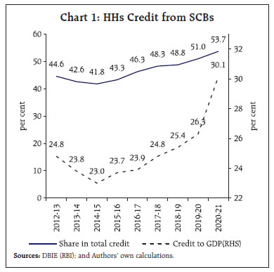 The share of non-banking credit by NBFCs, HFCs and others have grown in the recent period. The share of HH borrowings from all these institutions (SCBs, NBFCs, HFCs and Co-operatives banks) increased to 35.4 per cent of GDP in March 2020 from 32.9 per cent of GDP in March 2019. During the first phase of the pandemic-induced lockdown, households were striving hard for survival and borrowed to fulfil their basic needs due to the loss of jobs which brought up the ratio acutely to 38.5 per cent within a quarter (June 2020). The rising trend continued till March 2021 when it stood at 39.5 per cent, thereafter, the HH credit to GDP ratio started declining (Chart 2). 2.2 De composition of HHs’ Credit according to activity: Credit extended by SCBs to the HH sector consists of both personal and non-personal loans to Individuals including Hindu Undivided Family (HUF), un-incorporated enterprises such as proprietary and partnership concerns, Joint Liability Groups, NGOs, Trusts and Groups, etc. In March 2021, the personal loans constituted 25.9 per cent of the total bank credit and included mainly housing loans, vehicle loans, credit cards and educational loans; non-personal loans to HH sector constituted 27.8 per cent of the total bank credit and comprised mainly agricultural loans, industrial loans, and trade loans (Chart 3). 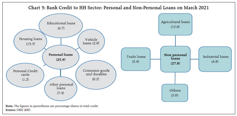
 The share of personal loans in total credit to HHs has risen steadily in recent years. Personal loans in HH credit increased to 48.1 per cent in March 2021 from 42.3 per cent in March 2019 i.e., the share rose remarkably by 5.7 percentage points during pandemic (Chart 4). The share of credit for agricultural activities reduced to 22.4 per cent in March 2021 as compared to 26.1 per cent during 2018-19 and trade remained around 10 per cent in total credit of HHs during the period of last 9 years. 2.3 Comparison with household borrowings position in BRICS nations India’s credit to GDP ratio of HHs is catching up with its peers among the emerging economies, however, there are marked heterogeneities in the internal forces driving them viz., HHs’ deposits, pattern of consumption/ expenditure, disposable income, and demographic dividend. A cross-country analysis based on the available data in World Bank and BIS database for Brazil, Russia, India, China, and South Africa (BRICS nations) is carried out to assess the empirical significance of such factors. 2.3.1 HH Credits and Deposits as percentage of GDP in BRICS The ratio of HH credit to GDP is lower in India than China but higher than the other three countries in BRICS as per BIS data (Chart 5). The ratio is relatively stable from 2015 onwards for India. Indian position appears moderate with respect to the credit to GDP ratio at 37.7 per cent as compared to China’s 61.7 per cent in 2020 but coinciding with South Africa from 2017 onwards. Recently, Brazil has also converged to India’s level. The data on HHs’ deposits for other BRICS countries are not available. Hence, as a proxy measure of liquidity, the ratio of broad money2 to GDP is considered. India’s broad money to GDP ratio is at a modest level among BRICS nations (Chart 6). The ratio in India has been relatively stable that may be considered as stable means for HHs to repay their loans besides fulfilling basic needs. 2.3.2 Working age population and unemployment rates in BRICS The credit demand of HHs may also depend upon demography viz., the proportion of working age population3 (WAP) in total population and the unemployment rate in the country. The comparable position across the BRICS nations is shown below in Charts 7 and 8. The proportion of working age population (WAP) in India is increasing unlike other BRICS countries and unemployment rate in India is quite lower than that prevailing in Brazil and South Africa. In year 2012, the Indian WAP was 64.8 per cent which gradually increased and reached at the level of 67.3 per cent in 2020. Considering the proportion of WAP along with the unemployment rates is important to analyse the credit demand by the HH sector from the perspectives of both the eligibility for credit and the economic burden of funding the basic needs. Increase in WAP with a constant rate of employment may help HHs to meet their needs better. 2.3.3 HH expenditure (as per cent of GDP) in BRICS In the pre-pandemic period, HH expenditure as percentage of GDP has exhibited relatively stable trend for India (Chart 9). The share of consumption expenditure by the sector in GDP was progressively rising and reached approximately 60 per cent in 2019 from 56.5 per cent in 2012. However, it experienced a sharp decline to 58.6 per cent in 2020. Nevertheless, India has a higher HH expenditure to GDP ratio than China and Russia. 3. HH borrowings: Sustainability Indicators 3.1 HH share in total domestic savings: Savings is an important indicator for assessing the sustainability of borrowings as it contributes to building up of assets which can be used for discharging future liabilities. In the recent period, liabilities of the HH sector have increased and their assets in the form of accumulated savings have also enlarged. The share of HH savings in Gross Domestic Savings (GDS) declined from 68.2 per cent in 2011-12 to 57.8 per cent in 2015-16 but increased thereafter to 78.5 per cent in 2020-21 (Chart 10). Of the total savings by the HH sector, 46.7 per cent are in the form of physical savings and 52.5 per cent in the form of financial savings in 2020-21(Chart 11) and these have become the most preferred source of savings for the sector.
3.2 Gross financial liability (GFL) to gross financial assets (GFA) ratio: The ratio of GFL to GFA, as a proxy for leverage, measures the strength of the financial balance sheet of HHs. In 2019-20, the financial liabilities of HH sector grew faster (12.2 per cent) than their financial assets (6.9 per cent), whereas in 2020-21 financial assets (17.5 per cent) grew more than the financial liabilities (11.3 per cent) in the sector (Chart 12). On a stock basis, gross financial liabilities remained less than 40 per cent of their gross financial assets during the last decade (Chart 13). Also, a sizable share of loans to HHs is in the form of housing loans (around 50 per cent), with the house itself working as the underlying collateral.
3.3 HH Credit to Deposit ratio: HH liabilities to SCBs and their assets with them can be captured in the ratio of their bank credit to bank deposit. The ratio provides insights into imbalances between credit and deposits; availability of liquidity and reliance on credit; and shifts in liquidity preferences and demand for credit. The ratio is important to assess the impact of any financial stress arising in the HHs’ balance sheet and spilling over to the banking sector. This ratio has been continually increasing in recent years and reached to 59.1 per cent in 2020-21, suggesting that the HH sector remains net lender to the banking sector despite the continuous increase in its CD ratio (Chart 14). Bank deposits remain the main form of HH savings among the major three components (Bank deposits, life insurance funds and currency) with a share of around 60 per cent (chart 15). 3.4 Composition of secured-unsecured loans and NPAs: Bank credit is the major component of HH liabilities. More than four fifths of HHs’ credit is secured and collateralised. In 2012-13 the share of secured loans in total HHs’ credit was 79 per cent which rose to 81 per cent in 2020-21 (Chart 16). NPA ratio for the sector indicates a rising trend in the recent past from 3.3 per cent in 2014-15 to 6.6 per cent in 2019-20 but reduced to 6 per cent in 2020-21 and it is falling well below the overall NPA ratio of 7.3 per cent in 2020-21 (Chart 17).
4. Data preparation, Methodology and Empirical Results Six factors viz., weighted average lending rates (WALR), change in the working age population (WAP), inflation (INF), HH deposits to GDP ratio (DEP_GDP), HH NPA ratio at first lag (HHNPA_lag1), private final consumption expenditure (PFCE) to GDP ratio as a proxy for HH expenditure to GDP ratio (HH_EXPGDP) are considered as covariates for HH credit to GDP (CR_TO_GDP), which is the HH sector borrowings indicator. Data are sourced from RBI (DBIE) and World Bank. Annual Data for all the regressors and HH credit to GDP ratio relate to the period 2002 – 2021. The ratio of change in the flow of financial liabilities of HH sector to its financial assets (HH FL/FA ratio) has been used for a longer time - period 1990-2020. Before investigating the relationship of these factors with the HH borrowings indicator, the pairwise correlations are computed among all the variables (Table 1, Annexure 1) and the problem of multicollinearity is identified. Consequently, all the chosen macro-economic factors were difficult to put in the analysis. Besides, this problem could have caused the estimates of coefficients to have higher variance and made them unreliable too. To avoid these consequences, principal component regression (PCR) is employed in the study (first suggested by Kendall, 1957). The basic idea under the technique is to reduce the dimension of the data while introducing orthogonality among the covariates using the principal component analysis (PCA). In the present study, it is applied with a sole purpose of using all the covariates without any loss of information and avoid misleading outputs due to multicollinearity. 4.1 Principal Component Regression (PCR) Analysis All the regressors are evaluated as correlated with HH borrowings indicator (CR_TO_GDP). PCR is applied and found significant at 5 per cent level. The model explains more than 80 per cent variation in HH credit to GDP ratio (i.e., CR_TO_GDP). Through reverse transformation, the original regression coefficients are obtained corresponding to original factors. The empirical results show that WALR is negatively related to HHs’ credit to GDP ratio as the cost of borrowing is expected to negatively affect the credit demand (H.O. et al ,2016). Household sector is more subtle to changes in interest rates (Debelle, 2004) and financial sector liberalisation along with increased private participation have also instilled strong competition among lenders compelling them to offer competitive interest rates on loans to attract potential borrowers (Fulwari ,2018). Change in working age population and inflation are also found inversely related to HHs’ borrowings. An increase in WAP in a stable labour market is expected to reduce the burden of financing consumption in a representative HH as its income gets boosted after the addition of more wage earners in the family. Further, higher inflation may increase interest rates, thus discouraging the demand for credit, but this is a short - term criteria. So, increase in both the covariates suppresses the need for credit in the short term. Lagged NPAs are also negatively related to the dependent variable as reduction in HHs’ NPA would encourage lenders (banks) to provide more credit to a wider range of HH borrowers. HH Deposits to GDP and PFCE_TO_GDP are found positively related to HHs’ credit to GDP ratio. The increase in deposit (financial assets) as a share of GDP may be taken as an increase in structural liquidity for banks which creates space for more leverage and the increase in consumption expenditure creates demand for credit. The diagnostic checking of the model is performed by plotting the standardized residuals against the predicted values of the HH borrowings indicator which is found as random indicating that the model has a best fit. 4.2 Sustainability Analysis Vulnerabilities are defined as pre-existing conditions that make the occurrence of an economic or financial crisis/stress more likely when an adverse shock hits (Dahlhaus and Lam, 2018). This definition is consistent with other academic literature (Christensen et al., 2015). Many researchers have previously analysed EMEs for assessing vulnerabilities. Their approaches are often similar, which is the Balance Sheet Approach introduced by IMF (IMF, 2002, 2004 and 2011). This article also employs the same idea but follows the approach of Pradhan (2018) which provides the simple algorithm to compute the vulnerability index on the scale of 0 to 10 and comprehensive interpretation of it. The vulnerability index (VI) has been computed for both indicators under our study - HH credit to GDP ratio and HH FL/ FA ratio during 2002-2021 and 1990–2020, respectively (Annexure 2). The latter ratio helps in assessing the flow side of imbalance in HH sector, if any. The entire period is divided suitably into different episodes. Five-year period starting with external payments crisis (1990-91 to 1994-95) and seven - year period covering 1995-96 to 2001-02. Rest of the episodes are constructed using the period prior to the Global financial crisis (GFC) (2002-03 to 2007-08), during GFC (2008-09 to 2011-12) and post GFC (2012-13 to 2019-20) for HH FL/HH FA ratio. Similarly, HH credit to GDP ratio (CR_TO_GDP) for the entire period from 2002 till 2021 is assessed for three episodes:2002-03 to 2007-08; 2008-09 to 2011-12; and 2012-13 to 2020-21. Since the annual values were not able to completely capture the volatility in the vulnerability index due to pandemic-induced mobility restrictions, therefore, additional computation of vulnerability index is performed using quarterly data of HH borrowings indicator (CR_TO_GDP) considering two mutually exclusive time epochs taken as pre pandemic (December 2018 to March 2020) and amid pandemic (June 2020 to September 2021), each comprising of six quarters. | Table 1: Computed Vulnerability Index for HH FL/ FA ratio | | Period | Vulnerability Index | | 1990-91 to 1994-95 | 5.21 | | 1995-96 to 2001-02 | 3.36 | | 2002-03 to 2007-08 | 4.91 | | 2008-09 to 2011-12 | 4.85 | | 2012-13 to 2019-20 | 4.81 | | Authors’ calculations. | Vulnerability index may take values from 0 to 10. Index value ranging from 5 to 10 indicates higher degree of financial risk/vulnerability, whereas the value ranging from 0 to 5 specifies absence of vulnerability. Both the vulnerability indices (based on the annual data) for the latest period were lower than 5, suggesting that HH borrowings in India does not indicate any sustainability concerns. In fact, other than the period from 1990-91 to 1994-95, the vulnerability index for HH financial liabilities to financial assets has always been less than 5, suggesting that HH borrowings have generally remained sustainable (Table 1). The value of the index was the lowest during the post external payments crisis episode (1995-96 to 2001-02). During the period of GFC (2008-09 to 2011-12), the index value at 4.85 did not pose any vulnerability for the HH sector. The vulnerability index (based on the quarterly data) during pandemic stood at 4.76, thus indicating unperturbed sustainability (Table 2). | Table 2: Computed Vulnerability Index for HH credit to GDP ratio | | Period | Vulnerability Index | | 2002-03 to 2007-08 | 4.89 | | 2008-09 to 2011-12 | 4.86 | | 2012-13 to 2020-21 | 4.66 | | Based on Quarterly data | | Pre-Pandemic (Dec-18 to Mar-20) | 4.96 | | Amid Pandemic (Jun-20 to Sep-21) | 4.76 | | Authors’ calculations. | 5. Conclusion This paper looked at the trends in borrowing of the households in India in order to understand what factors determine the household borrowing as well as examined its sustainability during periods of stress due to aggregate economic shocks. Our results show that household credit to GDP ratio has increased over the years. Ratio of household deposits to GDP and private final consumption expenditure are found to be positively related to household credit to GDP ratio whereas lending rate, inflation, lagged NPAs and increase in working age population are negatively associated with the same. The sustainability index shows that borrowing of Indian households remained within sustainable levels in the last three decades including the times of stress such as the pandemic. References Christensen, et al. (2015), “Assessing vulnerabilities in the Canadian financial system”, Bank of Canada, Financial system review, June 2015. Dahlhaus, T. and Lam, A. (2018), “Assessing Vulnerabilities in Emerging – Market Economies”, Bank of Canada Staff Discussion Paper 2018-13, October 2018. Debelle, G. (2004). Macroeconomic implications of rising household debt. BIS Quarterly Review, 3(153), 51–64. Retrieved from October 7, 2020. De Vaney, S. A. and Lytton, R. H. (1995),” Household Insolvency: A review of household debt repayment, Delinquency and bankruptcy”, Financial Services review, 4(2):137-156. Fulwari, A. (2018), “A review of literature on the determinants of the demand for home loans”, International education and research journal, E-ISSN No: 2454-9916 | Volume: 4 | Issue: 4 | April 2018. Ho, S. F. C., Yusof, J. M., & Mainal, S. A. (2016). Household debt, macroeconomic fundamentals and household characteristics in Asian developed and developing countries. The Social Science, 11(18), 4358–4362 IMF (2002), “A Balance Sheet Approach to Financial Crisis”, Policy development and Review Department, IMF, December 2002. IMF (2004), “Debt-Related Vulnerabilities and Financial Crises—An Application of the Balance Sheet Approach to Emerging Market Countries”, Policy development and Review Department, IMF, July 2004. IMF (2011), “Managing Volatility: A Vulnerability Exercise for Low-Income Countries”, Policy development and Review Department, IMF, Mar 2011. Kendall, M. G. (1957), “A Course in Multivariate Analysis”, Hafner, NY. Leigh, D. et al – IMF (2012), “Dealing with HH debt”, World Economic outlook: Growth resuming, Dangers remain, Ch 3, April 2012. Meniago, C. et al (2013), “What causes household debt to increase in South Africa”, Economic Modelling, 33 (2013) 482-492. Pradhan, K. (2018), “Assessment of India’s Fiscal and External Sector Vulnerability: A Balance Sheet Approach”, The Journal of Applied Economic Research, 12: 3 (2018): 308–332 Sage Publications Los Angeles/London/New Delhi/Singapore/Washington DC/Melbourne; DOI: 10.1177/0973801018768988 Ramadorai, P. (2017),” Indian HH Finance”, Committee report, Jul 2017. Samad, K.A. et al. (2020), “Determinants of household debt in emerging economies: A macro panel analysis”, Cogent Business & Management, 7: 1831765 (2020):1-14. SBI (2021), “FY21 GDP estimates at -8% may see upward revision: FY22 deposit growth of banking system reveals periods of alternate expansion & contraction”, ECOWRAP,13 (2021), pg 1-3. Zabai, A. (2017), “HH Debt: recent developments and challenges”, BIS quarterly review, Dec 2017.
Annexure 1 Pairwise Correlations are evaluated before applying the PCR and summarised in the following matrix. | Table 1 - Correlations | | | CR_TO_GDP | HHNPA_LAG1 | WALR | HH_EXPGDP | INF | WAP | DEP_GDP | | CR_TO_GDP | 1 | | | | | | | | HHNPA_LAG1 | -0.619 | 1 | | | | | | | WALR | -0.834 | 0.513 | 1 | | | | | | HH_EXPGDP | 0.321 | 0.833 | 0.302 | 1 | | | | | INF | -0.184 | -0.506 | 0.128 | -0.659 | 1 | | | | WAP | -0.379 | -0.119 | 0.497 | -0.301 | 0.449 | 1 | | | DEP_GDP | 0.874 | -0.564 | -0.825 | -0.347 | 0.375 | -0.267 | 1 | Principal components Regression (PCR) – Methodology: Let the linear regression model be given by: Y = βX + €, where Y is the vector of observations on dependent variable, X is the matrix of independent observations, β is the vector of regression coefficients and € is the vector of errors. First step is to standardize the variables, both dependent and independent variables. To perform PCR, we transform the independent variables to their principal components. Mathematically we write X’X = PDP’ = Z’Z, where D is the diagonal matrix of the eigen values of X’X, P is the eigenvector matrix of X’X, and Z is a data matrix (similar in structure to X) made up of the principal components. P is orthogonal so that P’P = I. We have created new variables Z as weighted averages of the original variables X. If we begin with variables X1, X2, and X3, we will end up with Z1, Z2, and Z3. Since these new variables are principal components, their correlations with each other are all zero. Severe multicollinearity will be detected by very small eigen values. To rid the data of the multicollinearity, we omit the components (the z’s) associated with small eigen values. Usually, only one or two relatively small eigen values will be obtained. For example, if only one small eigen value were detected on a problem with three independent variables, we would omit Z3 (the third principal component). When we regress Y on Z1 and Z2, multicollinearity is no longer a problem. We can then transform our results back to the X scale to obtain estimates of β. The mean squared error of these estimates is less than that for least squares. Mathematically, the estimation formula becomes Results: Principal components analysis is run for obtaining orthogonal set of data(regressors). Three components PC1, PC2 and PC3 together explained more than 90% variation in the data set. The choice of only three components is cross validated using the root mean squared error of prediction (RMSEP) (See the graph 1 below). RMSEP is declining till component 3 (i.e. Comp 3) and then it starts rising. Therefore, only first three components are chosen. Utilising the chosen components, the data of six covariates are transformed to the new data set with three variables that are orthogonal to each other. Linear regression is run for HH credit to GDP upon V1, V2 and V3 (the new regressors). PCR is found to be significant at 5% level of significance. Reverse transformation is done to get regression coefficients corresponding to each original variable. And the transformed regression model can explain 80.32 per cent of variation in HH credit to GDP. | Table 2: Regression Results | | Regressors | Regression Coefficients | Regression Statistics | | V1 | -3.416 | F (3,17) | 278.36 | | V2 | -5.264 | p value | 0.0355 | | V3 | -1.057 | Adjusted R-square | 0.8032 | Finally, the following regression model is obtained: Y= -1.713*WALR -1.097*WAP - 0.292*INF + 1.687*Dep_GDP - 0.69*HHNPA_LAG1 + 0.24* HHEXP_GDP Diagnostic checking of the applied PCR is also worked upon. For validation of PCR, plot of standardised residuals against Predicted Y values is utilised and found to be random which validates the PCR study.
Annexure 2 Methodology of Sustainability Analysis: The underlying methodology for computation of VI is as follows: Divide the entire period for each indicator in to small and relevant episodes of say 5-10 years suitably. To build VI, all observations Xi’s under each indicator are standardised into new Z scores as – where μ and σ are the mean and standard deviation of X during the episode. A Z-score close to zero indicates that an indicator is close to the average. A higher positive value implies a worse performance. To derive the index for each indicator, Z scores during each episode are transformed into cumulative distribution function of Normal Distribution and is so scaled that the values may range only between 0-10 with average score of 5. Finally, VI is obtained by taking the unweighted average of these values for each episode. An index ranging from 5 towards 10 indicates presence of higher degree of financial risk/ vulnerability.
|