Letter of Transmittal September 25, 2017 Dr. Viral V. Acharya,
Deputy Governor,
Reserve Bank of India,
Mumbai. Dear Sir, We herewith submit the Report of the Internal Study Group to Review the Working of the Marginal Cost of Funds Based Lending Rate (MCLR) System.
Executive Summary An internal Study Group was constituted by the Reserve Bank on July 24, 2017 to study the various aspects of the MCLR system from the perspective of improving the monetary transmission and exploring linking of the bank lending rates directly to market determined benchmarks. The constitution of the Study Group was announced in the Statement on Developmental and Regulatory Policies of the Reserve Bank of India on August 2, 2017. The Study Group submitted its report on September 25, 2017. The key findings emerging from the analysis undertaken by the Study Group and the recommendations made are set out below. Key Findings Monetary Transmission – the Base Rate and the MCLR Systems 2. A review of banks’ deposit and lending rates undertaken by the Study Group indicates that the transmission from the changes in the policy repo rate has been slow and incomplete under both the base rate and the marginal cost of funds based lending rate (MCLR) systems. The monetary transmission has improved since November 2016 under the pressure of large surplus liquidity in the system post demonetisation. While the transmission to interest rates on fresh loans was significant, it was muted to outstanding loans (base rate and MCLR). The transmission was also uneven across borrowing categories. Furthermore, the transmission to lending rates was asymmetric over monetary policy cycles – higher during the tightening phase and lower during the easing phase – irrespective of the interest rate system. For instance, the pass-through to outstanding loans from the repo rate was around 60 per cent during the tightening phase (July 2010 to March 2012), while it was less than 40 per cent during the subsequent easing phase (April 2012 to June 2013). 3. Analysis conducted by the Study Group suggests that banks deviated in an ad hoc manner from the specified methodologies for calculating the base rate and the MCLR to either inflate the base rate or prevent the base rate from falling in line with the cost of funds. These ad hoc adjustments included, inter alia, (i) inappropriate calculation of the cost of funds; (ii) no change in the base rate even as the cost of deposits declined significantly; (iii) sharp increase in the return on net worth out of tune with past track record or future prospects to offset the impact of reduction in the cost of deposits on the lending rate; and (iv) inclusion of new components in the base rate formula to adjust the rate to a desired level. The slow transmission to the base rate loan portfolio was further accentuated by the long (annual) reset periods. 4. Overall, monetary transmission has been impeded by four main factors: (i) maturity mismatch and interest rate risk in the fixed rate deposits but floating rate loan profile of banks; (ii) rigidity in saving deposit interest rates; (iii) competition from other financial saving instruments; and (iv) deterioration in the health of the banking sector. A major factor that impeded transmission was the maturity profile of bank deposits. Deposits with maturity of one year and above constituted 53 per cent of banks’ total deposits at end- March 2016, most of which were at fixed rates of interest. Another source of weak transmission was rigidity in interest rates on banks’ saving deposits, which remained notoriously stubborn even as the policy repo rate and interest rates on term deposits moved in either direction. The third factor, which hindered monetary transmission was the competition that banks faced from other saving instruments. It appears that banks were reluctant to reduce interest rates sharply for fear of losing deposits to other financial saving instruments such as mutual funds and small saving schemes. Although bank deposits have some distinct advantages in the form of stable returns (vis-à-vis mutual fund schemes) and liquidity (vis-à-vis small saving schemes), bank deposits are in a disadvantageous position in terms of tax-adjusted returns in comparison with these schemes. Banks, therefore, often appeared to be reluctant to reduce interest rates on deposits in line with the reduction in the policy rate by the Reserve Bank. These factors imparted rigidity to the liability side of banks’ balance sheet. Finally, empirical analysis suggests that the extent of responsiveness of interest earnings and interest expenses to the changes in the policy repo rate is broadly the same, making the net interest margins (NIMs) impervious to monetary policy changes. The deterioration in the health of the banking sector and the expected loan losses in credit portfolios induced large variability in spreads in pricing of assets, severely impacting monetary transmission as banks’ NIMs have remained broadly unchanged in the face of large stressed assets. Thus, rigidities on the liability side such as longer-term maturity pattern of deposits with fixed interest rates, along with the expected loan losses on the asset side, have been reflected in higher pricing on the asset side, i.e., lending rates. Spreads charged over the Base Rate and the MCLR 5. Median spreads charged over the MCLR by all bank groups remained broadly stable in the case of fresh rupee loans from April 2016 to December 2016. However, median spreads charged rose sharply in January 2017. Median spreads of public and private sector banks declined by June 2017. However, while the median spread of private sector banks declined to the pre-January 2017 level, the median spread of public sector banks remained significantly above the pre-January 2017 level. 6. Spreads charged by private sector banks on fresh rupee loans were consistently the largest, followed by public sector banks and foreign banks. Spreads charged varied significantly across banks and also temporally. Spreads of foreign banks were relatively more volatile than those of public and private sector banks. 7. The transmission from the reduction in the MCLR to lending rates occurred with a lag. In the case of private sector banks, it took almost six months for the transmission from the lower MCLR to actual lending rates. However, in the case of public sector banks, the transmission was not complete even after six months. 8. The transmission to interest rates on outstanding rupee loans was significantly lower than on fresh rupee loans. The median spread in the case of outstanding rupee loans remained significantly higher than that of fresh rupee loans, reflecting the dominance of base rate loan portfolio in outstanding loans and lagged interest rate reset (normally one year) for the existing borrowers under the MCLR system. Spreads on outstanding loans were also more volatile than those on fresh loans. 9. Being an internal benchmark, the MCLR is expected to vary across banks. The spread over the MCLR could also vary from bank to bank due to idiosyncratic factors. However, variations in the spreads across banks appear too large to be explained based on bank- level business strategy and borrower-level credit risk. In particular, spreads charged by some banks seem excessively and consistently large. The analysis suggests that the spreads were mostly changed arbitrarily by banks for similar quality borrowers. While the spread over the MCLR was expected to play only a small role in determining the lending rates by banks, it turned out to be the key element in deciding the overall lending rates. This has made the entire process of setting lending interest rates by banks opaque and impeded the monetary transmission. 10. That many banks tended to charge the spreads over the MCLR arbitrarily is evident from a special study of select banks conducted by the Study Group. The key findings of the study are: (i) large reduction in MCLR was partly offset by some banks by a simultaneous increase in the spread in the form of business strategy premium ostensibly to reduce the pass-through to lending rates; (ii) there was no documentation of the rationale for fixing business strategy premium for various sectors; (iii) many banks did not have a board approved policy for working out the components of spread charged to a customer; (iv) some banks did not have any methodology for computing the spread, which was merely treated as a residual arrived at by deducting the MCLR from the actual prevailing lending rate; and (v) the credit risk element was not applied based on the credit rating of the borrower concerned, but on the historically observed probability of default (PD) and loss given default (LGD) of the credit portfolio/sector concerned. Recommendations 11. The recommendations made by the Study Group are detailed below. 12. The lower transmission from the policy rate to the base rate loan portfolio was mainly due to the reason that banks followed different methods to calculate the base rate. Banks, therefore, could be advised to re-calculate the base rate immediately by removing/readjusting arbitrary and entirely discretionary components added to the formula. It needs to be ensured that the calculation of the base rate is not compromised in any way. The methodology adopted by banks should be subject to a regular supervisory review. 13. In the absence of any sunset clause on the base rate, banks have been quite slow in migrating their existing customers to the MCLR regime. Most of the base rate customers are retail/SME borrowers. Hence, the banking sector’s weak pass-through to the base rate is turning out to be deleterious to the retail/SME borrowers in an easy monetary cycle. To address this concern, besides immediate recalculation of base rates (as recommended in para II.15), banks may be advised to allow existing borrowers to migrate to the MCLR if they so choose to do without any conversion fee or any other charges for switchover on mutually agreed terms. However, after the adoption of an external benchmark from April 1, 2018 as recommended by the Study Group (refer paras IV.43 - IV.45), banks may be advised to migrate all existing benchmark prime lending rate (BPLR)/base rate/MCLR borrowers to the new benchmark without any conversion fee or any other charges for switchover on mutually agreed terms within one year from the introduction of the external benchmark, i.e., by end-March 2019. 14. The Study Group recommends that it should be made mandatory for banks to display prominently in each branch the base rate/MCLR (tenor-wise) and the weighted average lending rates on loans across sectors separately for loans linked to the base rate and the MCLR. The same information should also be hosted prominently on each bank’s website. The Reserve Bank could prescribe the format and the manner in which a minimum set of standardised data needs to be displayed in branches/hosted on banks’ websites. The Indian Banks’ Association (IBA), or any other agency considered appropriate by banks, could also disseminate bank-wise information on its website in the same manner in which each bank is required to disseminate information on its own website so as to facilitate easy comparison of lending rates across sectors and banks. The same system of dissemination of information on the benchmark and the weighted average lending rate could be followed under the external benchmark system recommended by the Study Group (see paras IV.43 - IV.45). 15. An evaluation of 13 possible candidates [weighted average call rate (WACR), collateralised borrowing and lending obligation (CBLO) rate, market repo rate, 14-day term repo rate, G-sec yields, T-Bill rate, certificates of deposit (CD) rate, Mumbai inter- bank outright rate (MIBOR), Mumbai inter-bank forward offer rate (MIFOR), overnight index swap (OIS) rate, Financial Benchmark India Ltd. (FBIL) CD rates, FBIL T-Bill rates and the Reserve Bank’s policy repo rate)] suggests that no instrument in India meets all the requirements of an ideal benchmark. Each instrument has certain advantages as also limitations. After carefully analysing the pros and cons of 13 possible candidates as a benchmark, the Study Group narrowed down its choice to three rates, viz., a risk-free curve involving T-Bill rates, the CD rates and the Reserve Bank’s policy repo rate. The T-Bill rate and the CD rate1 were further assessed on three parameters, viz., (i) correlation with the policy rate; (ii) stability; and (iii) liquidity. The Study Group is of the view that the T-Bill rate, the CD rate and the Reserve Bank’s policy repo rate are better suited than other interest rates to serve the role of an external benchmark. 16. The T-bill rates are risk free and also transparent. They also have a reliable term money market curve. CD rates relate to the credit market directly in the sense that banks could meet their marginal requirement of funds from this market. CDs also have a reliable term money market curve. Unlike the T-Bill market where the money market term curve is available up to 12 months, in the CD market, the term curve is generally up to six months (and up to 9 months occasionally). The main challenge in using either T-bill rates or CD rates as the benchmark is that the current level of market depth in the T-Bill and CD markets can make such benchmarks potentially susceptible to manipulation. Also, T-Bill rates may at times reflect fiscal risks which will automatically get transmitted to the credit market when used as a benchmark. CD rates also have their own limitations - high sensitivity to liquidity conditions, credit cycles, and seasonality. Liquidity in the CD market is inadequate because there are no large and frequent issuances by a sufficient number of highly rated banks. The Reserve Bank’s policy repo rate has the primary advantage that it is robust, reliable, transparent and easy to understand. It reflects the appropriate rate for the economy at any point in time based on the MPC’s assessment of macroeconomic conditions and the outlook. With the repo rate as the benchmark, the transmission of the repo rate changes to lending rates of banks will be quick, direct and strong. The repo rate as a benchmark, however, can constrain future changes in the monetary policy framework. Banks also have limited access to funds at the repo rate. Being an overnight rate, the repo rate also lacks a term structure. 17. The Study Group recognised that internal benchmarks such as the base rate/MCLR have not delivered effective transmission of monetary policy. Arbitrariness in calculating the base rate/MCLR and spreads charged over them has undermined the integrity of the interest rate setting process. The base rate and MCLR regimes are also not in sync with global practices on pricing of bank loans. Given that there has not been much forward movement on the external benchmark even after seventeen years from the time when it was first allowed in the country, the development of an external benchmark would need guidance from the Reserve Bank. Accordingly, there is a need for switching over to one of the external benchmarks recommended by the Study Group, after wider public debate and taking into account the feedback from all stakeholders. Given the scope of arbitrariness under the MCLR system, however, the switchover to an external benchmark needs to be pursued in an expedient and time-bound manner. 18. The Study Group recommends that all floating rate loans extended beginning April 1, 2018 could be referenced to one of the three external benchmarks selected by the Reserve Bank after receiving and evaluating the feedback from stakeholders. 19. The Study Group is of the view that the decision on the spread over the external benchmark should be left to the commercial judgment of banks. However, the spread fixed at the time of sanction of loans to all borrowers, including corporates, should remain fixed all through the term of the loan, unless there is a clear credit event necessitating a change in the spread. 20. Banks may be encouraged to accept deposits, especially bulk deposits at floating rates linked directly to one of the three external benchmarks selected by the Reserve Bank after receiving the feedback from stakeholders as recommended by the Study Group. 21. The Study Group recommends that the corporates and banks be encouraged to actively manage interest rate risks once the external benchmark is introduced. It should also help deepen the IRS market, going forward. 22. Finally, but equally importantly, the reset clause, which is typically one year, impedes monetary transmission as the pass-through of monetary policy changes to existing floating rate loans is delayed. The Study Group, therefore, recommends that the periodicity of resetting the interest rates by banks on all floating rate loans, retail as well as corporate, be reduced from once in a year to once in a quarter.
Chapter I
Introduction I.1 The efficacy of monetary policy depends on the magnitude and the speed with which policy rate changes are transmitted to the ultimate objectives of monetary policy, viz., inflation and growth. With the deepening of financial systems and growing sophistication of financial markets, most monetary authorities use interest rate as the key instrument to achieve the ultimate objectives of monetary policy. Adjustments in the policy interest rate, for instance, directly impact short-term money market rates which then transmit the monetary policy impulses across financial markets and maturity spectrum, including banks’ deposit and lending rates. These, in turn, influence consumption, saving and investment decisions of firms and households, which ultimately influence aggregate demand, and hence, output and inflation. The interest rate channel of transmission – supported by liquidity management operations – is the leading channel of transmission in several countries, including many emerging market economies. I.2 In a bank dominated system like India, the transmission to banks’ lending rates is the key to the successful implementation of monetary policy. However, the issue of transmission from the policy rate to banks’ lending rates has all along been a matter of concern for the Reserve Bank. The transmission to banks’ lending rates has been impeded by a variety of factors, the major one being the opacity in the process by which the banks set their lending interest rates. To address this concern, the Reserve Bank has refined the interest rate setting methodology of banks from time to time. I.3 In 1994, when the lending interest rates were deregulated, the Reserve Bank prescribed that banks should disclose their prime lending rates (PLRs), which will be the interest rate charged for the most creditworthy borrowers. Keeping in view the request from banks that the PLR should be converted into a reference or benchmark rate for banks, the Reserve Bank advised banks in April 2003 to announce a Benchmark PLR (BPLR) with the approval of their boards. The dominance of sub-BPLR lending, however, defeated the very purpose for which the BPLR system was introduced. I.4 The Reserve Bank replaced the BPLR system with the base rate system in July 2010 under which the actual lending rate charged to borrowers was the base rate plus borrower- specific charges. However, the flexibility accorded to banks in the determination of cost of funds – average, marginal or blended cost – caused opacity in the determination of lending rates by different banks and rendered the assessment of monetary transmission difficult. I.5 The Reserve Bank instituted a new lending rate system for banks – the marginal cost of funds based lending rate (MCLR) system – effective April 1, 2016 with a view to improving transmission. The BPLR, the base rate and the MCLR were internal benchmarks set by each bank for pricing of credit. However, unlike the BPLR and the base rate, the formula for computing the MCLR was prescribed by the Reserve Bank. Since 2000, banks are also free to price credit linked to external benchmarks. However, the share of rupee loans linked to external benchmarks has been miniscule. I.6 The experience with the MCLR system has not been satisfactory, even though it has been an improvement over the base rate system. The transmission has remained uneven in terms of its pace and magnitude: (i) across the sectors of the economy; (ii) between deposit and lending rates; and (iii) between fresh rupee loans and outstanding rupee loans. The base rates of different banks, in particular, have remained rigid since introduction of the MCLR. While the extent of change in base rate may not necessarily mirror the changes in the MCLR, the rigidity of the base rate is a matter of concern for efficient transmission of monetary policy to the real economy. Also, a large portfolio of banks’ loans – about one-fourth – continues at the base rate and does not show the expected sensitivity to changes in the policy rate of the Reserve Bank. I.7 The spread, as measured by the difference between the lending rate and the 1-year MCLR, which was expected to be by and large stable, has shown large variations from month to month, from bank to bank and from sector to sector. While some variability in the spread over the MCLR was expected, large variations in the spreads are difficult to explain. Accordingly, an internal Study Group was constituted to study the various aspects of the MCLR system and explore linking of bank lending rates directly to market- determined benchmarks. The announcement of the Constitution of the Study Group was made in the Statement on Developmental and Regulatory Policy of the Reserve Bank on August 2, 2017. The Study Group comprised the following officials: Dr. Janak Raj,
Principal Adviser,
Monetary Policy Department | Chairman | Smt. Parvathy V. Sundaram,
Chief General Manager-in-Charge,
Department of Banking Supervision | Member | Shri S.S. Barik,
Chief General Manager-in-Charge,
Department of Banking Regulation | Member | Shri T. Rabi Sankar,
Chief General Manager,
Financial Markets Regulation Department | Member | Shri R. Gurumurthy,
Chief General Manager,
Financial Stability Unit | Member | Terms of Reference of the Study Group I.8 The terms of reference for the Study Group were as under: -
To study whether the MCLR has achieved the objective for which it was introduced. -
To look into the practices followed by banks for fixing the spread over the MCLR. -
To suggest appropriate modification in the MCLR system with a view to strengthening the monetary transmission. -
To make any other recommendation with regard to setting of interest rates by banks for improving the monetary transmission. I.9 The Study Group was required to submit the report within two months (Annex I.1). Acknowledgements I.10 The Study Group expresses its sincere gratitude to Dr. Viral V. Acharya, Deputy Governor, for giving it an opportunity to work on the critical issue of MCLR as also for sharing his perspectives on the challenges to transmission under the MCLR regime and the evolving benchmark related reforms internationally. The Study Group also thanks Dr. M.D Patra, Executive Director, for his continuous guidance, which helped the Study Group to understand the transmission related challenges in the conduct of monetary policy in India. I.11 The Secretariat of the Study Group comprised three officials of the Monetary Policy Department (MPD), viz., Shri Sitikantha Pattanaik, Director, Shri Muneesh Kapur, Director and Shri A.K. Mitra, Director. I.12 The Study Group is appreciative of the feedback it received from the representatives of select banks with whom the Study Group held discussions on August 22, 2017 (Annex I.2). I.13 The Study Group benefitted in the form of comments/suggestions received from Dr. D.P. Rath, Adviser, MPD; Shri K. Rajkumar, Adviser, MPD; Dr. Praggya Das, Director, MPD; Dr. Nishita Raje, Director, Department of Banking Regulation (DBR); Shri P.K.Seth, General Manager, DBR; Shri Indranil Chakraborty, General Manager, Financial Stability Unit; Shri S.R. Pattanaik, General Manager, Department of Banking Supervision; and Shri Manoj Kumar, Deputy General Manager, Financial Markets Regulation Department. I.14 The Study Group wishes to place on record its deep appreciation for the resource persons from MPD – Shri S.M. Lokare, Assistant Adviser; Shri Rajesh Kavediya, Assistant Adviser; Dr. Harendra Behera, Assistant Adviser; Shri Joice John, Assistant Adviser; and Smt. Abhilasha, Assistant Adviser – who worked on specific aspects covered in the report. The Study Group also thankfully acknowledges the administrative and data-related support provided by Smt. Rita Maheshwari, Manager; Shri M.H. Ahuja, Assistant Manager; Smt. S.R. Apte, Senior Special Assistant; Smt. G.S. Parab, Senior Special Assistant; Shri P.V. Khadye, Senior Special Assistant; and Shri Nilesh Dalal, Assistant. I.15 The Report is organised in five chapters. Chapter II examines whether the MCLR has achieved the objective for which it was introduced. The performance of the base rate system is also assessed in this Chapter. Chapter III looks into the practices followed by banks for fixing the spread over the base rate/MCLR. Chapter IV explores market rates as the possible candidates for an external benchmark for pricing of floating rate loans. Chapter V sets out the recommendations of the Group for strengthening the monetary transmission.
Chapter II
Monetary Transmission: The Base Rate and the MCLR Systems I. Introduction II.1 In India, banks are the main conduits through which monetary impulses are transmitted to the real economy. Hence, it has been the endeavour of the Reserve Bank to strengthen the monetary transmission by focussing on the design of the lending interest rates of the banking system. It was in keeping with this that the Reserve Bank introduced the base rate system in July 2010, which was replaced by the marginal cost of funds based lending rate (MCLR) system in April 2016. This chapter undertakes a detailed review of the working of the base rate and the MCLR systems with a view to (i) assessing how monetary transmission has worked under these two regimes; and (ii) understanding the various factors that impede the monetary transmission. II. Banks’ Lending Rate Systems since the Early 1990s: An Overview Prime Lending Rate (PLR) System II.2 After the introduction of the financial sector reforms in the early 1990s, the Reserve Bank initiated various measures to progressively deregulate the interest rates – both deposit and lending rates. In a major initiative in October 1994, the Reserve Bank deregulated lending rates for credit limits over Rs.2 lakh. Banks were also required to declare their prime lending rates (PLR), i.e., the interest rate charged for the most creditworthy borrowers. The PLR was to be computed taking into account factors such as cost of funds and transaction costs, and was expected to act as a floor for lending above Rs.2 lakh. The experience with the working of the PLR system, however, was not satisfactory mainly for two reasons: (i) both the PLR and the spread charged over the PLR varied widely across banks; and (ii) the PLRs of banks were rigid and inflexible in relation to the overall direction of interest rates in the economy. Benchmark Prime Lending Rate (BPLR) System II.3 In order to improve transparency and ensure appropriate pricing of loans, the Reserve Bank advised banks in April 2003 to announce Benchmark PLRs (BPLRs). Banks were required to compute BPLRs taking into account the cost of funds, operational costs, minimum margin to cover regulatory requirements (provisioning and capital charge), and profit margin. The BPLR system also fell short of its original intent of enhancing transparency and serving as the reference rate for pricing of loan products. The transparency aspect, in particular, was hit by the fact that a large part of the lending actually took place at interest rates below the announced BPLRs. The share of sub-BPLR lending was as high as 77 per cent in September 2008, concentrated at long-term tenors (above three years), rendering it difficult to assess the transmission of policy rate changes of the Reserve Bank to lending rates of banks. The residential housing loans and the consumer durable loans were outside the purview of the BPLR. As such, sub-BPLR lending became a major distortion in terms of cross-subsidisation across borrower categories. The Base Rate System II.4 The drawbacks of the BPLR system called for a further refinement of the lending rate system and the base rate system was introduced in July 2010. Under this framework, each bank was required to announce its base rate, taking into account, inter alia, the costs of borrowed funds (Table II.1). The base rate was to be the minimum rate for all loans, except for some specified categories1. The actual lending rate charged to the borrowers was to be the base rate plus borrower-specific charges. The base rate system, with a link to the banks’ cost of funds, was expected to facilitate better pricing of loans, enhance transparency in lending rates and improve the assessment of the transmission of monetary policy. In practice, flexibility accorded to banks in the determination of cost of funds – average, marginal or blended cost – caused opacity in the determination of lending rates by banks and clouded an accurate assessment of the speed and strength of the transmission. Moreover, the discrimination in the pricing of credit between the new and old customers continued, as banks often adjusted the spread over the base rate to benefit the new borrowers. | Table II.1: The Base Rate and the MCLR Methodologies – A Comparison | Base Rate System
(effective July 1, 2010) | MCLR System
(effective April 1, 2016) | (a) Cost of (Borrowed) Funds (b) Negative Carry on cash reserve ratio (CRR)/statutory liquidity ratio (SLR) (c) Unallocatable Overhead Cost (d) Average Return on Net Worth Base Rate = a+b+c+d - One base rate for each bank
- Any benchmark could be used
- Frequency: Quarterly review with Board’s approval
- No prescribed reset period
- Fixed rate loan – not below base rate
| (a) Marginal Cost of Funds
[= 92% of Marginal Cost of Deposits and Other Borrowings + 8% of Return on Net Worth] (b) Negative Carry on CRR (c) Operating Cost (d) Tenor Premium/Discount MCLR = a+b+c +d - Tenor-linked benchmark
- No discretion allowed on benchmark
- Frequency: Monthly on a pre-announced date
- Reset period indicated in contract. Maximum one year reset period for floating rate loans
- Fixed rate loan over 3 year tenor – exempt from MCLR.
| Marginal Cost of Funds based Lending Rate (MCLR) System II.5 The weaknesses and rigidities observed with the transmission under the base rate system were intended to be addressed through marginal cost of funds based lending rate (MCLR) system for new loans, effective April 1, 2016. The base rate system, however, was expected to be in operation concomitantly for the loans already contracted, pending their maturity or a shift to the MCLR system at mutually agreeable terms between the bank and the borrower. The parallel operation of the MCLR and the base rate systems has considerably impacted the transmission in respect of the outstanding loans linked to the base rate as detailed later in this report. II.6 The MCLR consists of four components: (a) marginal cost of funds [marginal cost of borrowings (comprising deposits and other borrowings) and return on net worth]; (b) negative carry on account of cash reserve ratio (CRR); (c) operating costs; and (d) term premium (Table II.1). Under the MCLR system, banks are required to determine their benchmark lending rates linked to their marginal cost of funds [unlike the base rate system where banks had the discretion to choose between the average cost or the marginal cost (or blended cost) of funds]. As such, lending rates were expected to be more sensitive to the changes in the policy rate under the MCLR system vis-à-vis its predecessor (the base rate). The MCLR plus spread is the actual lending rate charged to a borrower. The spread comprises only two components, viz., business strategy and credit risk premium. III. Transmission under the Base Rate and the MCLR Systems: An Analysis II.7 The MCLR regime has been in operation for almost 18 months and the transmission under the system has, like the earlier systems, remained below expectations. The extent and pace of reduction in MCLRs have been uneven since April 2016, and a large part of the observed transmission was due to the demonetisation-induced surge in the balances under current and savings accounts (CASA). While the transmission to interest rates on fresh rupee loans has been significant, it has been partial to existing loans (both at the base rate and outstanding MCLR) (Table II.2 and Chart II.1). Fresh Rupee Loans -
As against the total reduction in the policy repo rate of 200 basis points (bps) between December 2014 and August 2017, the weighted average lending interest rate (WALR) on fresh rupee loans declined by 193 bps. A significant part of transmission (96 bps), however, occurred post-demonetisation. -
Between January 2015 and August 2017, the median base rate of banks declined by only 75 bps vis-à-vis 158 bps decline in the banks’ median term deposit rate, and 195 bps decline in the weighted average domestic term deposit rate (WADTDR). -
Between April 1, 2016 (when the MCLR became operational) and October 2016 (i.e., prior to demonetisation), the reduction in the 1-year median MCLR (15 bps) trailed significantly the reduction in the median term deposits rate (around 27 bps) and the policy repo rate (50 bps). The median base rate remained almost unchanged during this period. -
During the post-demonetisation period (November 2016 onwards), while the weighted average term deposit rate (69 bps) and the median MCLR (80 bps) declined significantly, the median base rate of banks declined only marginally by 14 bps (Table II.2). | Table II.2: Transmission from the Policy Repo Rate to Banks’ Deposit and Lending Rates | | (Variation in percentage points) | | Period | Repo Rate | Term Deposit Rates | Lending Rates | | Median Term Deposit Rate | WADTDR | Median Base Rate | Median MCLR (1-year) | WALR - Outstanding Rupee Loans | WALR - Fresh Rupee Loans | | August 2017 over end-December 2014 | -2.00 | -1.58 | -1.95 | -0.75 | * | -1.25 | -1.93 | | August 2017 over April 1, 2016 | -0.75 | -0.86 | -1.04 | -0.15 | -0.95 | -0.61 | -0.95 | | Memo: | | Pre-Demonetisation | | January 2015 to October 2016 | -1.75 | -0.99 | -1.26 | -0.61 | * | -0.75 | -0.97 | | April 1, 2016 to October 2016 | -0.50 | -0.27 | -0.35 | -0.01 | -0.15 | -0.11 | 0.01 | | Post Demonetisation | | November 2016 to August 2017 | -0.25 | -0.59 | -0.69 | -0.14 | -0.80 | -0.50 | -0.96 | WADTDR: Weighted Average Domestic Term Deposit Rate.
WALR: Weighted Average Lending Rate.
MCLR: Marginal Cost of Funds based Lending Rate.
*: MCLR system was put in place in April 2016.
Source: Special Monthly Return VIAB, RBI. |
Outstanding Rupee Loans II.8 The transmission to outstanding rupee loans was significantly lower than the policy rate. As against the cumulative policy rate cut of 200 bps during December 2014 and August 2017, the weighted average lending rate (WALR) declined by 125 bps, of which 50 bps reduction was post-demonetisation. The transmission to outstanding rupee loans was also weak in relation to the reduction of 195 bps in the weighted average term deposit interest rate and notwithstanding a significant increase in low cost CASA deposits (Box II.1). Box II.1: Demonetisation: Impact on Transmission As banks credited the depositors’ accounts with the value of surrendered demonetised bank notes, post-demonetisation, CASA deposits of banks rose sharply. The share of the low cost CASA deposits in total bank deposits increased from 35.2 per cent in October 2016 to 40.6 per cent in March 2017, before declining to 38.6 per cent in June 2017 (Table A). The surge in deposits during November- December 2016 led to a large surplus liquidity – with a peak of near Rs.8 trillion – with the banking system. With credit demand remaining sluggish, banks reduced their term deposit rates significantly towards end-December 2016/early-January 2017; interest rates on saving deposit accounts, however, were left unchanged. In an environment of surplus liquidity, weak credit demand, lower cost of term deposits, and a surge in low cost CASA deposits, banks announced a large cut in their MCLRs in January 2017. Thus, a large part of the transmission was facilitated by a large surplus liquidity on account of demonetisation. | Table A: Share of CASA in Aggregate Deposits – Scheduled Commercial Banks # | | As on the last Reporting Friday | Share (Per cent) | | March 2013 | 33.1 | | March 2014 | 32.8 | | March 2015 | 32.7 | | March 2016 | 34.1 | | October 2016 | 35.2 | | March 2017 | 40.6 | | June 2017 | 38.6 | | #: Excluding Regional Rural Banks. | | Transmission: Bank Group-wise II.9 The transmission was uneven across bank groups. The transmission to the WALR on outstanding rupee loans was relatively better in the case of private sector banks vis-à-vis public sector banks and foreign banks (Table II.3). | Table II.3: Transmission – Weighted Average Lending Rate*: Bank Group-Wise | | (Variation in Percentage Points) | | Period | Repo Rate | Public Sector Banks | Private Sector Banks | Foreign Banks | SCBs# | | January 2015 to June 2017 | -1.75 | -1.09 | -1.52 | -1.14 | -1.17 | Pre-Demonetisation
(January 2015 to October 2016) | -1.75 | -0.70 | -1.00 | -0.98 | -0.75 | Post-Demonetisation
(November 2016 to June 2017) | 0.00 | -0.39 | -0.52 | -0.16 | -0.42 | *: Relates to outstanding rupee loans. #: excluding Regional Rural Banks.
Source: Special Monthly Return VIAB, RBI. | Transmission: Borrowing Categories-wise II.10 The extent of transmission was also asymmetric across sectors (Table II.4). The decline in the WALR on outstanding loans during December 2014-June 2017 was greater for large industrial entities (despite higher NPAs) vis-à-vis retail housing and retail vehicle loans. Even in an environment of easy monetary policy, interest rates on credit cards increased by almost 100 bps, touching almost 40 per cent per annum. | Table II.4: Weighted Average Lending Rates*: Sector-wise | | (Per cent) | | End-Month | Rupee Export Credit | Trade | Industry (Large) | Profes-sional Services | Infra-struc-ture | Personal Other@ | Personal Education | MSMEs | Personal Housing | Personal Vehicle | Agriculture | Personal Credit Card | | 1 | 2 | 3 | 4 | 5 | 6 | 7 | 8 | 9 | 10 | 11 | 12 | 13 | | Dec-14 | 12.16 | 13.09 | 12.95 | 12.39 | 13.05 | 14.24 | 12.90 | 13.05 | 10.76 | 11.83 | 10.93 | 37.86 | | Mar-15 | 12.04 | 13.07 | 12.80 | 12.46 | 12.89 | 13.94 | 12.87 | 12.91 | 10.99 | 11.62 | 10.96 | 37.88 | | Mar-16 | 11.46 | 12.50 | 12.36 | 11.81 | 12.06 | 13.90 | 12.48 | 12.25 | 10.56 | 11.65 | 10.74 | 38.00 | | Mar-17 | 10.98 | 11.59 | 11.57 | 11.21 | 11.80 | 12.85 | 11.70 | 11.88 | 9.78 | 11.05 | 10.95 | 39.02 | | Jun-17 | 9.78 | 11.41 | 11.28 | 10.91 | 11.59 | 12.85 | 11.53 | 11.75 | 9.59 | 10.87 | 10.78 | 38.88 | | Variation (Percentage Points) | | Jun-17 over Dec14 | -2.38 | -1.68 | -1.67 | -1.48 | -1.46 | -1.39 | -1.37 | -1.30 | -1.17 | -0.96 | -0.15 | 1.02 | | Jun-17 over Oct-16 | -1.00 | -0.45 | -0.36 | -0.65 | -0.30 | -0.13 | -0.87 | -0.48 | -0.41 | -0.58 | -0.10 | -0.13 | *: Relates to outstanding rupee loans, at which 60 per cent or more business is contacted.
@: Other than housing, vehicle, education and credit card loans.
Source: Special Monthly Return VIAB, RBI. | Transmission: Monetary Policy Cycles II.11 The transmission to lending rates over different monetary policy cycles was asymmetric. It was somewhat higher during the tightening phase of monetary policy and lower during the easing phase, irrespective of the interest rate regime (Table II.5). | Table II.5: Transmission – Tightening and Easing Policy Cycles | | (Variation in Percentage Points) | | Phase | Repo Rate | Public Sector Banks | Private Sector Banks | Foreign Banks | SCBs | | DR | LR-O | LR-F | DR | LR-O | LR-F | DR | LR-O | LR-F | DR | LR-O | LR-F | | Tightening | | | | | | | | | | | | | | | April 2004- September 2008 | 3.0 | 2.41 | 0.09 | - | 2.96 | -0.60 | - | 2.95 | -1.90 | - | 2.53 | -0.23 | - | | Easing | | | | | | | | | | | | | | | October 2008- February 2010 | -4.25 | -1.43 | -1.84 | - | -2.47 | -1.56 | - | -3.63 | -2.00 | - | -1.74 | -1.81 | - | | Tightening | | | | | | | | | | | | | | | March 2010- June 2010 | 0.50 | - | - | - | - | - | - | - | - | - | - | - | - | | July 2010- March 2012 | 3.25 | 2.06 | 2.29 | - | 2.72 | 1.29 | - | 3.58 | 1.03 | | 2.22 | 2.03 | - | | Easing | | | | | | | | | | | | | | | April 2012- June 2013 | -1.25 | -0.40 | -0.60 | - | -0.73 | -0.08 | - | -0.84 | 0.39 | | -0.46 | -0.44 | - | | Tightening | | | | | | | | | | | | | | | July 2013- December 2014 | 0.75 | -0.10 | -0.35 | -0.16 | -0.10 | 0.01 | 0.45 | 0.35 | -0.46 | 0.09 | -0.09 | -0.28 | 0.05 | | Easing | | | | | | | | | | | | | | | January 2015- March 2016 | -1.25 | -0.93 | -0.58 | -0.98 | -0.85 | -0.88 | -1.12 | -0.88 | -0.72 | -0.68 | -0.91 | -0.64 | -0.98 | | April 2016- October 2016 | -0.50 | -0.34 | -0.12 | 0.05 | -0.34 | -0.12 | 0.02 | -0.27 | -0.26 | -0.47 | -0.35 | -0.11 | 0.01 | | November 2016- June 2017 | 0 | -0.57 | -0.39 | -0.97 | -0.63 | -0.52 | -1.24 | -0.51 | -0.16 | -0.57 | -0.57 | -0.42 | -0.98 | DR: Weighted Average Domestic Term Deposit Rate.
LR-O: Weighted Average Lending Rate on Outstanding Rupee Loans.
LR-F: Weighted Average Lending Rate on Fresh Rupee Loans.
Source: Special Monthly Return VIAB, RBI. | II.12 The above analysis suggests that the transmission to fresh rupee loans was significant, especially post demonetisation. However, the transmission to outstanding rupee loans, especially base rate portfolio, was significantly lower. The transmission was uneven across bank groups and sectors. It was also asymmetric across monetary policy cycles. Working of the Base Rate System: Some Concerns II.13 The Study Group conducted a study of the methodology of the base rate calculation of a few major banks. The study revealed that the banks took recourse to many ad hoc adjustments in the methodology, which either inflated the base rate or prevented the base rate from falling in line with the cost of funds (Box II.2). Box II.2: Base Rate Methodology of Select Banks: Key Findings The key findings of a study of four major banks (two public sector banks and two private sector banks) revealed the following discrepancies: -
For calculating the cost of deposits/funds, one major public sector bank took average of the card rates of retail term deposits (7 days to 1 year) only, ignoring fully the low cost CASA deposits [current account (no interest cost) and saving account (interest cost of 4 per cent)], which formed a significant portion of the total deposits of the bank. -
Another major public sector bank kept the base rate unchanged between September 2016 and March 2017 even as its cost of deposits declined by around 40 bps. The bank, however, increased its return on net worth by almost 45 bps; as a result, the base rate remained unchanged. -
The actual base rate worked out by one major private sector bank in March 2017 was almost 80 bps higher than suggested by the base rate formula. In April 2017, the bank’s actual base rate was close to the formula, as the bank tweaked the formula-based base rate, by adding two new components to the formula. -
The cost of deposits of another private sector bank declined by almost 120 bps between Q3:2016-17 and Q4:2016-17, but the bank offset a large chunk of this decline by increasing its return on net worth by almost 100 bps. As a result, the decline in the base rate was just a fraction of the decline in the cost of deposits. | II.14 Even 15 months after the introduction of the MCLR regime, a sizable part of loans (around 30 per cent) is still at the base rate. The progress of migration of borrowers from the base rate system to the MCLR regime has been tardy (Box II.3). Box II.3: Migration of Borrowers to the MCLR Regime – Why is the Progress Slow? Though the base rate system replaced the BPLR system with effect from July 1, 2010, and the MCLR system replaced the base rate system from April 1, 2016, some past loans based on the BPLR system and the base rate system have continued in the system. The switchover from one system to another can take place only on mutually agreed terms between the bank and the borrower. Customers who shifted from the BPLR regime to the base rate regime were charged a spread higher than the borrowers who entered the base rate system directly, leading to issues of discrimination amongst existing and new customers. Banks insist on charging the same interest rate (in nominal terms) if a customer wishes to switch from the base rate regime to the MCLR regime. In other words, an existing customer who wants to convert his base rate linked loan to a MCLR linked loan would be required to pay a higher spread than the new borrower even though all other factors that go into the pricing of credit (risk profile, maturity, and loan type) remain the same. This discrimination with the existing borrowers is a direct consequence of a modest downward revision in the base rate as against a much sharper decline in the MCLR during the most recent easing cycle. In an easy monetary policy environment, where the average cost of deposits is higher than the marginal cost, the lenders – motivated to attract new business – prefer to pass on the benefits of lower cost of marginal funds primarily to the new customers, while they continue to charge higher interest rates from the existing customers. In other words, while banks provide all the incentives to new borrowers to attract them, they deny such benefits to existing borrowers. This way, banks are able to grow their new business and protect their balance sheets from the interest rate risk, and maintain their NIMs. Hence, banks have little incentive to nudge their existing base rate borrowers to switch to the MCLR system. Banks have also been slow in reducing their base rates and in some cases the base rate was arbitrarily inflated, as alluded to before. As a result, floating rate loans contracted during the base rate regime still carry higher rates of interest than the floating rate loans contracted during the MCLR regime. In fact, the initial wedge that existed between the base rate and MCLR in April 2016 has widened further. The MCLR guidelines did not provide for any sunset clause for loans linked to the BPLR/base rate. While existing loans based on the BPLR/base rate system could run till their maturity, the existing borrowers desirous of switching to the MCLR system, before expiry of the existing contracts, were given an option to migrate on mutually agreed terms. Further, in terms of existing guidelines, no fee was allowed to be charged for switch over from the BPLR system to the base rate system. However, in the case of a shift of BPLR/base rate linked loans to MCLR linked loans, fees can be charged. It is significant that: (i) banks do not widely publicise the option to shift to MCLR linked loans; (ii) banks can charge a fee for facilitating the shift; and (iii) there is no reduction in the interest rate immediately following the shift. For all these reasons, customers are either ignorant of the option or are discouraged from shifting to MCLR linked loans. | Recommendations II.15 The lower transmission from the policy rate to the base rate loan portfolio was mainly due to the reason that banks followed different methods to calculate the base rate. Banks, therefore, could be advised to re-calculate the base rate immediately by removing/readjusting arbitrary and entirely discretionary components added to the formula. It needs to be ensured that the calculation of the base rate is not compromised in any way. The methodology adopted by banks should be subject to a regular supervisory review. II.16 In the absence of any sunset clause on the base rate, banks have been quite slow in migrating their existing customers to the MCLR regime. Most of the base rate customers are retail/SME borrowers. Hence, the banking sector’s weak pass-through to the base rate is turning out to be deleterious to the retail/SME borrowers in an easy monetary cycle. To address this concern, besides immediate recalculation of base rates as recommended in paragraph II.15, banks may be advised to allow existing borrowers to migrate to the MCLR if they so choose to do without any conversion fee or any other charges for switchover on mutually agreed terms. However, after the adoption of an external benchmark starting from April 1, 2018 as recommended by the Study Group (refer paras IV.43 - IV.45), banks may be advised to migrate all existing benchmark prime lending rate (BPLR)/base rate/MCLR borrowers to the new benchmark without any conversion fee or any other charges for switchover on mutually agreed terms within one year from the introduction of the external benchmark, i.e., by end-March 2019. Working of the MCLR System: Some Concerns II.17 The implementation of the MCLR regime at the bank level raises some concerns (Box II.4). Box II.4: The MCLR Regime in Practice – A Study of Select Banks: Major Findings Several banks have resorted to a number of practices which have been at variance with the guidelines prescribed by the Reserve Bank and have hampered the smooth implementation of the MCLR regime. A special study conducted by the Study Group suggests several disconcerting practices followed by banks, which, among others, include the following: -
Even after 18 months of its introduction, in most banks, only around 40 per cent of the corporate portfolio and one fourth of retail portfolio are under the MCLR regime. -
A few banks made little effort to migrate small and retail customers from the base rate system to the MCLR regime, as there was no proper dissemination of switchover option through the branches of the banks or their websites. -
A number of banks levied a one-time switchover fee on migration of advances from the base rate to the MCLR regime. Moreover, it was observed that the effective interest rate burden on the borrower remains the same even after switching to the MCLR regime from the base rate regime. In a few cases, interest rates were raised by as much as 300 basis points. -
The calculation methodology followed by banks raises some concerns: -
Some banks had inflated the return on net worth (RoNW), which was neither in tune with market conditions nor with their track record. This was done presumably to bring MCLR close to the prevailing base rate of the concerned bank. -
Capital Asset Pricing Model (CAPM) was arbitrarily used with varying assumptions to compute the cost of capital to arrive at the RoNW. -
Some banks did not have a cost accounting system for their loan products and loaded the entire operational cost – components such as clearing house rent, corporate social responsibility spending – which were not directly associated with lending, thereby overstating the operating costs. -
The definition of operating cost followed by some banks was not in accordance with the guidelines prescribed by the Reserve Bank. As per the guidelines, the operating cost component was to be used for computing MCLR at the bank-wide level, while the operating cost used by some banks was different for various loan products. -
Computation of core and volatile portion of saving deposit accounts in some banks was at variance with the guidelines. -
A large portion of increase in CASA deposits post-demonetisation was not considered as a core component of deposits by a bank. -
A bank computed the MCLR for one-year tenor, even though it was not the single largest maturity bucket for the total funds. -
Some banks considered a lower part of saving deposits as core deposits for computation of marginal cost of funds. -
Some banks determined tenor premia/discounts subjectively in the absence of any method/market benchmarks. -
Some banks have not reviewed tenor premia/discounts determined since March 2016. -
In the case of one bank, loan pricing was determined based on fund transfer pricing instead of being determined as per the mandated base rate/MCLR methodology. | MCLR and Lending Rates II.18 Different components of MCLR vary across banks reflecting: (i) differences in the composition and maturity profile of their liabilities – current, savings and time deposits - and the extent of reliance on retail vis-à-vis wholesale customers, which has a bearing on the cost of funds; (ii) divergences in the operating cost arising out of differences in the use of technology, quality of human capital and the geographical spread of bank branches; and (iii) the return on net worth expected by banks. II.19 What matters for monetary policy is the transmission from the policy rate to actual lending rates, which consist of MCLR and the spread charged over the MCLR, as alluded to earlier. Thus, the transmission to MCLRs may not necessarily lead to transmission to lending rates, if banks make offsetting adjustments in spreads charged along with the changes in their MCLRs. It is noteworthy that in the case of fresh loans, spreads charged by SCBs narrowed between April 2016 and June 2017. However, in the case of outstanding loans, spreads widened, suggesting that banks adjusted the spreads charged over MCLRs upwards such that the reduction in lending rates was lower than that in MCLRs. This was mainly on account of widening of spreads by public sector banks and foreign banks, while spreads charged by private banks declined (Chart II.2). Thus, for assessing the effectiveness of monetary transmission, it is important to study the MCLR and the spreads charged separately. 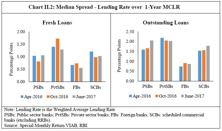 II.20 While the practices followed by banks with regard to setting of spreads over the base rate/MCLR are detailed in the next chapter, the main factors that appeared to have impeded monetary transmission are detailed in the following section. IV. Factors Impeding Monetary Transmission II.21 A number of factors impede a fuller and speedier pass-through from the Reserve Bank’s policy repo rate to banks’ deposit and lending rates. Maturity Profile of Deposits and Loans II.22 As at end-March 2016, more than half of the deposits of commercial banks were in a maturity bucket of ‘one year and above’ and almost 20 per cent of the deposits were in a maturity bucket of ‘five years and above’ (Chart II.3)2. During the easy cycle of monetary policy, banks reduced their deposits rates on new deposits, which lowered the marginal cost of funds. However, more than 50 per cent of deposits with a maturity of one year and above continued to attract high interest rates. The high cost and long maturity deposits kept the average cost of deposits elevated, which, in turn, appeared to have constrained banks from lowering their lending interest rates. The constraint was felt more acutely by public sector and private sector banks as they held more than 20 per cent of their deposits with maturity five years and above; foreign banks held only a negligible share of their deposits with maturity of five years and above. 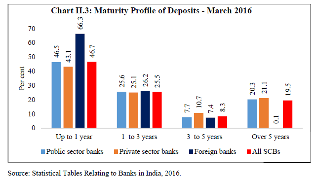 II.23 The rigidity in interest rate on savings accounts (detailed in the followingsection) observed during 2011-17 was another major factor that kept the average (asalso marginal) cost of funds high during the easy phase and low during the tight phase. II.24 While almost all bank deposits were at fixed rates, most of banks’ loans (almost 80 per cent) were at floating rates. The maturity profile of loans and advances extended by public sector and private sector banks was skewed towards longer-term loans (one year and more), while that of foreign banks was towards shorter loans (one year and less) (Chart II.4). The asymmetry in the interest rate setting (fixed for deposits and largely floating for loans) combined with a substantial part of deposits in longer maturities appeared to have constrained banks from quickly transmitting the policy rate cuts to their lending rates, especially on past loans. 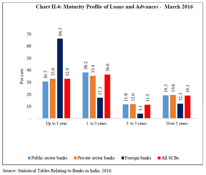 II.25 Base rate-linked loans currently account for around 30 per cent of the outstanding bank credit, with wide variation across bank groups (negligible in the case of foreign banks and 41 per cent in the case of public sector banks). The base rate loan portfolio also varied widely within the same bank group (Table II.6). A sizable proportion of loans at the base rate combined with the slow pace of reduction in the base rate impaired the pace of monetary transmission to interest rates on outstanding loans. | Table II.6: Bank Credit at Floating Rates: Benchmark-based Shares | | (Per cent to total credit) | | Group | BPLR | Base Rate | MCLR | LIBOR | | Mar-17 | Jun-17 | Mar-17 | Jun-17 | Mar-17 | Jun-17 | Mar-17 | Jun-17 | | Public Sector Banks (21) | | | | | Minimum | 0.04 | 0.03 | 34.39 | 28.11 | 18.23 | 27.06 | - | - | | Maximum | 15.69 | 13.25 | 62.67 | 56.55 | 56.54 | 62.56 | - | - | | Median | 1.40 | 1.48 | 47.23 | 41.39 | 31.57 | 39.51 | - | - | | Private Sector Banks (20) | | | | Minimum | 0.00 | 0.01 | 7.32 | 5.01 | 20.50 | 22.38 | 0.61 | 1.78 | | Maximum | 2.30 | 1.75 | 53.00 | 42.00 | 100.00 | 100.00 | 7.37 | 9.13 | | Median | 0.39 | 0.24 | 32.38 | 25.19 | 44.43 | 50.37 | 3.99 | 5.46 | | Foreign Banks (28) | | Minimum | 0.00 | 0.00 | 0.00 | 0.00 | 0.00 | 0.00 | 0.00 | 0.00 | | Maximum | 0.55 | 0.44 | 71.00 | 27.11 | 100.00 | 100.00 | 60.12 | 80.21 | | Median | 0.00 | 0.00 | 9.04 | 0.07 | 49.74 | 52.75 | 16.78 | 23.20 | | Scheduled Commercial Banks (69) | | Minimum | 0.00 | 0.00 | 0.00 | 0.00 | 0.00 | 0.00 | 0.00 | 0.00 | | Maximum | 15.69 | 13.25 | 71.00 | 56.55 | 100.00 | 100.00 | 60.12 | 80.21 | | Median | 0.78 | 0.44 | 34.41 | 26.43 | 36.68 | 43.42 | 13.89 | 18.36 | | Source: Special survey of commercial banks conducted by RBI. | II.26 The transmission to outstanding rupee loans was also adversely impacted as one fifth of outstanding bank credit was at fixed rates at end-June 2017, with wide dispersion across bank groups and also within bank groups (Table II.7). The proportion of fixed rate loans was around 35 per cent in the case of foreign banks and relatively moderate (15 per cent) in the case of public sector banks. Fixed rate loans weakened the overall transmission of monetary policy. | Table II.7: Share of Fixed Rate Loans | | (Per cent in total credit) | | | PSBs | PvtSBs | Foreign Banks | SCBs | | | Mar-17 | Jun-17 | Mar-17 | Jun-17 | Mar-17 | Jun-17 | Mar-17 | Jun-17 | | Minimum | 0.46 | 0.86 | 0.00 | 0.00 | 0.00 | 0.00 | 0.00 | 0.00 | | Maximum | 27.54 | 28.80 | 100.00 | 100.00 | 100.00 | 100.00 | 100.00 | 100.00 | | Median | 15.00 | 15.27 | 24.00 | 26.47 | 41.59 | 34.50 | 19.02 | 19.15 | Note: Data pertain to 69 scheduled commercial banks (21 PSBs, 20 private sector banks and 28 foreign banks).
Source: Special survey of commercial banks conducted by RBI. | II.27 Even in the case of floating rate loans, the benefit of the realised reduction in the MCLR was available mostly to fresh rupee loans after a lag, of about one year, since interest rates on floating rate loans were reset at fixed periodicity, which is typically one year. This was one of the reasons that the reduction in WALR on outstanding rupee loans between April 2016 and August 2017 was only 61 bps vis-à-vis a reduction of almost 100 bps in the one-year median MCLR rate. Recommendation II.28 The reset clause, which is typically one year, impedes monetary transmission as the pass-through of monetary policy changes to existing floating rate loans is delayed. The Study Group, therefore, recommends that the periodicity of resetting the interest rates by banks on all floating rate loans, retail as well as corporate, be reduced from once in a year to once in a quarter. Rigidity in Saving Deposit Rates II.29 Saving deposits constitute more than three-fourth of CASA balances of commercial banks (Chart II.5). II.30 In the run up to the deregulation of savings deposit interest rates in India in 2011, banks had expressed apprehension that the deregulation would lead to a rate war among banks. In contrast, however, interest rates on saving deposits of major banks remained sticky at 4 per cent (until very recently), barring some minor adjustments by some smaller and private and foreign banks and some new banks. This is despite the fact that monetary policy switched from a tightening mode to an accommodative mode twice over the period and term deposit interest rates moved in either direction (Chart II.6). Between October 2011 and June 2017, 11 SCBs, with a market share of 4.1 per cent in aggregate deposits, increased their saving deposit rates in a range of 10 bps to 300 bps. 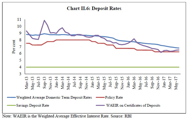 II.31 It was only on July 31, 2017 that the State Bank of India (SBI), the largest bank in the country, slashed interest rate on saving deposits by 50 bps to 3.5 per cent on balances of Rs.1 crore and below. The decline in the share of CASA balances in the post-March 2017 period (reversing a part of the sharp rise witnessed in November- December 2016, due to demonetisation) (see Box II.1) pushed up banks’ cost of funds and 'would have necessitated an increase in MCLRs. However, this option was not easy given the low credit offtake. Hence, some banks, led by the SBI, decided to reduce the interest rate on saving deposits. In all, 28 banks, accounting for a market share of 82.8 per cent in aggregate deposits, reduced their savings deposit rates in a range of 25 bps to 150 bps during August–September 2017. Despite the recent reduction in the saving deposit interest rate by some banks, the spreads between savings deposit interest rate on the one hand, and term deposit interest rates on the other, have remained wide (Chart II.7). 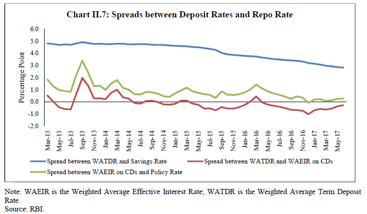 II.32 The observed rigidity in the interest rate on saving deposits can be due to the following factors. First, saving deposit balances are almost 30 per cent of banks’ total deposits. Therefore, any change in the interest rate on these balances is applicable to all outstanding balances, which has an immediate and sizable impact on banks’ cost of funds. In contrast, changes in interest rates on time deposits impact only incremental deposits contracted at the new rate, the impact of which on the overall cost of funds is limited. Hence, banks chose not to raise interest rate on saving deposits during the tightening phase of monetary policy. II.33 Second, some banks with whom the Study Group held discussions indicated that saving deposits entail high operating costs. Given the higher overall costs, most banks chose not to increase their interest rates on saving deposits during the tightening phase of monetary policy (2011-12). Since banks did not increase the interest rate on saving deposits during the tightening phase, it appeared that there was reluctance by banks to reduce saving deposit rates during the easing phase of monetary policy. II.34 It is intriguing that saving deposit interest rates remained sticky even when the policy repo rate and banks’ own term deposit interest rates moved in either direction significantly after deregulation of the saving deposit interest rate in October 2011. On the one hand, banks appear reluctant to reduce interest rate on saving deposits as they face competition from mutual funds and small savings. On the other hand, banks chose not to raise saving deposit interest rates when all other interest rates in the system moved up significantly during 2011-12. Had banks raised saving deposit interest rates during the tight monetary policy phase, it would not have been so difficult to reduce the interest rates on such deposits during the easy monetary policy cycle. That the saving deposits carry high operational cost cannot be a good enough reason for banks not to change interest rate on such deposits in line with other interest rates. This is not to suggest that the saving deposit interest rates need to be changed to the same extent as term deposit interest rates. However, there is certainly a strong case for adjusting such rates regularly in line with other interest rates in the system. Competitive Pressures from other Financial Saving Instruments II.35 While modulating their deposit rates in response to monetary policy signals, commercial banks also take into account returns available to depositors on alternative instruments of financial savings. In particular, banks in India take into account interest rates on small saving schemes and returns available on mutual fund schemes. II.36 Small savings by the government compete directly with bank deposits. Although the government has been periodically adjusting downwards the interest rates on these instruments since April 2016, these still remain well above those being offered by the banking system. Interest rates on small saving schemes also remain higher than the rates based on the formula indicated by the Government in its press release of February 16, 2016 (Table II.8). The tax adjusted rate of return on select small savings schemes (viz., 5-year time deposits, public provident fund, national savings certificates and senior citizen’s savings scheme) are even higher. A large interest rate differential in favour of small savings can lead to a significant migration of deposits away from banks, with an adverse impact on banks’ lending capacity. Hence, this appeared to have constrained banks from reducing their deposit interest rates in consonance with the changes in the monetary policy rate, especially during the easing phase of monetary policy. | Table II.8: Interest Rates: Select Small Saving Schemes and Commercial Bank Term Deposits | | (Per cent) | | Small Savings | Commercial Banks | Difference (7 - 3) (Percentage Points) | Difference (7 - 4) (Percentage Points) | | Small Saving Scheme | Maturity (years) | Formula based Rate of Interest* | Govern-ment Announced Rate of Interest* | Maturity (years) | Interest Rate Range (August 2017) | Median (August 2017) | | 1 | 2 | 3 | 4 | 5 | 6 | 7 | 8 | 9 | | Saving Deposit | - | | 4.00 | - | 3.50-7.25 | 4.00 | 0.00 | 0.00 | | Term Deposits | | | | | | | | | | 1 Year | 1 | 6.2 | 6.8 | 0-1 | 2.00-9.75 | 5.32 | -0.88 | -1.48 | | 2 Year | 2 | 6.3 | 6.9 | 1-2 | 3.50-10.50 | 6.75 | 0.45 | -0.15 | | 3 Year | 3 | 6.4 | 7.1 | 2-4 | 4.75-10.50 | 6.63 | 0.23 | -0.47 | | 5 Year | 5 | 7 | 7.6 | 4-5 | 5.00-10.50 | 6.55 | -0.45 | -1.05 | | Senior Citizens Saving Scheme | 5 | 7.7 | 8.3 | 5 | 5.50-11.00 | 7.05 | -0.65 | -1.25 | *: Applicable for July-September 2017.
Source: Government of India, Special Monthly Return VIAB, RBI. | II.37 Mutual funds have recently emerged as a major source of competition to the banks for financial savings. Assets under management (AUM) of mutual funds grew at a (compound) rate of 18.3 per cent per annum during the 10-year period 2007-17, outpacing the growth of 15.3 per cent in bank deposits during the same period. As a result, assets under management of mutual funds as percentage of bank deposits (outstanding) increased in the recent period (Chart II.8). II.38 Funds mobilised under debt oriented schemes also increased sharply. During 2016-17, inflows under such schemes were about 20 per cent of incremental deposits mobilised by banks. The surge of inflows into mutual funds has continued in 2017-18 so far. Returns on mutual fund debt oriented schemes are generally higher than interest rates on bank deposits. II.39 The investor base of mutual funds is also becoming more broad-based3. There were 59 million accounts at end-July 2017. Of these, 48 million accounts related to the equity, equity-linked savings scheme (ELSS) and balanced schemes, with mostly retail investors. Individual investors (including high net worth individuals) accounted for almost one-half of total assets of the industry (48.1 per cent) as of July 2017 (Chart II.9). II.40 Banks face competition from mutual funds mainly from debt oriented and liquid schemes, especially because such schemes carry tax benefits. In the case of bank deposits (savings or fixed), interest income gets taxed at the applicable marginal slab tax rate of the depositor (the peak rate is 30 per cent at present). On the other hand, returns from the long-term debt funds (held for more than three years) are taxable at 20 per cent with indexation benefit and 10 per cent without indexation (again well below the peak marginal income tax rate of 30 per cent). II.41 Investments in banks’ fixed deposits with a lock-in period of 5 years as well as in the equity linked saving schemes (ELSS) of mutual funds enjoy tax benefits under Section 80C of the Income Tax Act. However, the overall tax benefits are loaded in favour of mutual funds. First, the lock-in period associated with the ELSS is lower (3 years) than that of bank deposits (5 years). Second, ELSS returns are tax free, while interest income on deposits is taxable at the applicable tax slab in the hands of the depositor. II.42 In the case of fixed deposits, there is a penalty associated with premature withdrawal. Mutual funds, on the other hand, offer higher liquidity and exit load is typically charged only for withdrawal under a year (most liquid funds do not charge an exit load). Thus, mutual fund schemes are also liquid like bank deposits. II.43 Falling interest rates on bank deposits and tax benefits in favour of mutual funds have made mutual fund investments highly attractive relative to bank deposits. This appeared to have constrained banks from reducing their interest rates on fresh deposits, blunting even the first leg of the transmission (from the policy repo rate to bank deposit rates). The weaker first stage transmission, in conjunction with other rigidities noted in this chapter, then dampens the second leg of the transmission (from the bank funding costs to lending rates). II.44 A level-playing field for all the competing financial saving instruments is necessary for enhanced monetary transmission. Any tax benefit in favour of a particular saving instrument distorts the risk-return perception of a saver, which is not conducive for developing a balanced and diversified financial system. Deterioration in Asset Quality of Banks II.45 There has been a significant deterioration in the asset quality of banks in recent years. Gross non-performing assets (NPAs) of scheduled commercial banks (SCBs) increased more than three times from 2.9 per cent (of gross advances) in March 2012 to 9.6 per cent in March 2017. Total stressed assets (i.e., NPAs plus restructured assets) increased sharply from 7.5 per cent to 12.0 per cent over the same period (Chart II.10). II.46 The increase in stressed assets, however, was largely concentrated in public sector banks (Chart II.11). II.47 Since a sharp deterioration in the asset quality has implications for their net interest income and profitability, banks could be expected to be reluctant to fully pass on the reduction in their MCLRs to their lending rates. Significantly, NIMs of public sector banks have declined marginally since 2012, reflecting rising NPAs. NIMs of private sector banks, on the other hand, have risen, suggesting more pricing power. Although NIMs of foreign banks have declined – albeit from a fairly high level – they are still the highest among all bank groups. Return on assets (RoA) of PSBs has declined, reflecting higher provisioning/write-offs against bad assets. On the other hand, RoA of private sector banks and foreign banks has remained broadly stable over past six years (Chart II.12). Net Interest Margins and Monetary Policy Stance II.48 In principle, fluctuations in interest rates are expected to have some impact on banks’ net interest income, given the maturity and interest rate mismatches. Cross-country evidence, however, indicates that banks’ net interest margins are impervious to interest rate cycles. This appears to be true for both conventional and unconventional monetary policies. Aggregate net interest margins in the US have been near-constant for the past six decades (1955-2013), despite substantial maturity mismatch and wide variation in interest rates4. This could be due to banks' market power in deposit markets, which allows banks to pay deposit rates that are low and relatively insensitive to interest rate changes. Banks hedge these liabilities by investing in long-term assets, whose interest payments are also relatively insensitive to interest rate changes. II.49 Turning to the experience with the unconventional monetary policies, policy interest rates have been close to zero and even negative in some euro area countries and Japan over the last few years. In these countries, the available evidence, albeit limited, indicates that despite negative interest rates, banks have been able to largely protect their NIMs5. In the euro area and Japan, NIMs have declined somewhat, though not significantly. In Denmark and Sweden, margins have remained stable, and in Switzerland they even increased somewhat. Although deposit rates have been largely sticky in these countries, banks have been able to maintain their NIMs due to a variety of factors: ‘tiering system’ by the respective central banks for the remuneration of reserve balances (Japan and Switzerland); incomplete pass-through of negative rates to lending rates (Denmark); a counterintuitive increase (although temporary) in mortgage rates (Switzerland); and, more generally, cheaper wholesale funding. II.50 Regression analysis indicates that banks in India, like those in other countries, are able to insulate their net interest margins from the monetary policy actions (Annex II.1). The following key findings emerged from the empirical analysis. -
Although policy repo rate changes have an impact on banks’ interest income as well as interest expenses, the impacts are largely off-setting leaving no statistically significant impact on their net interest margins. -
The impact of repo rate changes on banks’ interest income and expenses is substantially lower than proportional. An increase of 100 bps in the policy repo rate is estimated to increase banks’ interest income ratio (relative to assets) as well as interest expenses ratio (relative to assets) by only about 50 bps. -
Banks are able to match the interest rate sensitivities of their assets and liabilities. This finding is in line with that in the US banking system, where banks are “able to engage in substantial maturity transformation without bearing the interest rate risk it would normally entail”.6 II.51 The finding of less than proportional sensitivity of interest expenses to the variations in the repo rate in the Indian context can be explained by the following factors: (a) extreme rigidity in interest rates on saving accounts (accounting for nearly 30 per cent of total bank deposits) throughout the sample period; (b) almost all term deposits are at fixed interest rates, which reduce the sensitivity of interest expenses to repo rate changes; and (c) reluctance at times on the part of banks to change their interest rates on new deposits in the face of competition from small savings and mutual funds. II.52 Similarly, the low sensitivity of interest income to repo rate changes for the Indian banking system can be explained by the following factors: (a) a substantial share of lending (over one-fourth) is still at the base rate, which is mostly priced on average (and not marginal) cost of funds and the base rate has declined only moderately in recent quarters; (b) the annual resetting periodicity (which delays the decline in actual lending rates) and an arbitrary upward adjustment of spreads reduce the response of interest income to policy rate changes; and (c) almost one-fifth of banks’ assets are in government securities (as mandated by the SLR requirement) with a large part being in the ‘held to maturity’ category, making the earnings less sensitive to repo rate changes. II.53 These findings have important implications for monetary policy transmission. First, banks in India have been able to protect their NIMs in the face of large stressed assets. This would suggest that the deterioration in asset quality of banks impacted monetary transmission. Second, if banks’ NIMs were not impacted by the monetary policy changes, it would suggest that rigidities on the liability side of banks’ balance sheets were reflected in pricing on the asset side of banks, thereby impeding monetary transmission. II.54 Although the recourse by banks to the repo window is limited, the empirical evidence suggests that the Indian banking system has been effective in managing the monetary policy cycles well. This would suggest that the policy repo rate has the potential to serve as an external benchmark for pricing of loans (as well as deposits).
Chapter III
Spreads Charged over the Base Rate and the MCLR:
A Review of Practices followed by Banks I. Introduction III.1 Internal benchmarks for pricing of rupee loans1 such as the base rate and the marginal cost of funds based lending rate (MCLR) include all those cost elements which can be clearly identified and are common across borrowers2. The actual lending rate includes the base rate/MCLR plus a spread representing borrower-specific charges. Under the base rate system, borrower-specific charges include credit risk, tenor premium and allocable portion of the operating costs. The spread charged to an existing borrower is not allowed to be increased except on account of deterioration in the credit risk profile of the borrower or a change in the tenor premium. In the case of MCLR system, banks charge a spread for two elements, viz., business strategy and credit risk. The spread charged to an existing borrower cannot be increased except on account of deterioration in the credit risk profile of the borrower. Any change in the business strategy element under the MCLR system affects only the new borrowers. III.2 While the spread should ideally reflect business strategy and credit risk, the discretion available to the banks in fixing spreads can potentially be used in a manner that could impair transmission. Examining how spreads are fixed by the banks is essentially a data intensive process. The analysis in this chapter is based on two approaches: (a) a deep dive into bank-wise and sector-wise spreads based on data reported by banks to the Reserve Bank; and (b) special studies conducted by the Study Group on practices followed by select banks in fixing the spreads. III.3 In the case of floating rate fresh rupee loans linked to MCLR, any change in the MCLR should be reflected in actual lending rates of the borrowers, unless there is a change in the business strategy of the bank and/or credit risk profile of the customer. In the case of existing borrowers, any change in the MCLR should be reflected in actual lending rates unless it is neutralised by a corresponding change in the credit risk profile. III.4 To clearly understand the practices followed by banks in setting the spreads over MCLR/base rate, data have been analysed for the period from April 2016 to June 2017 in four dimensions. First, the analysis is carried out based on the median rate in respect of each bank group. However, the median rate alone does not tell the whole story as it is concentrated at the middle. It also does not give an idea about the variability and the outliers. For understanding these aspects, box plot charts3 have been used which depict changes in the distribution of spreads charged by banks over time. This is the second dimension of the analysis. The third dimension of the analysis is based on the temporal distribution of spreads of each bank, again using the box plot charts. While a useful tool of analysis, box plot charts do not capture how the spreads of individual banks have moved over a period of time. For this purpose, data relating to 14 select major banks (six public sector, four private sector and four foreign banks) have been analysed. The analysis is carried out separately for fresh rupee loans and outstanding rupee loans (comprising both fixed rate and floating rate loan portfolio). The analysis based on outstanding loans, however, is undertaken only along the first two dimensions. II. Fresh Rupee Loans: Spreads charged by Banks Analysis based on Median Spreads III.5 An examination of monthly data on the median spread4 of bank groups indicates that spreads charged by public sector banks and private sector banks declined during April-December 2016. The decline was more pronounced in the case of public sector banks with the WALR-F falling faster than the decline in the median MCLR in an environment of low credit growth and ample liquidity (Chart III.1). In January 2017, spreads charged by public sector banks and private sector banks, however, widened significantly following the sharp reduction in the 1-year MCLR on account of a spurt in CASA deposits as also reduction in term deposit rates post demonetisation. This lowered the marginal cost of funds and hence, the MCLRs of both the bank groups. 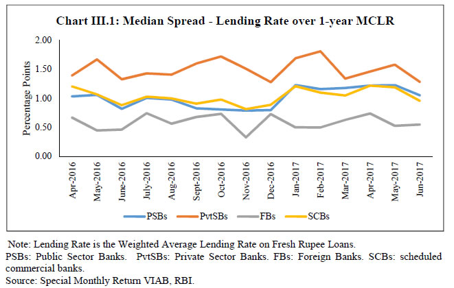 III.6 Banks, however, passed on the reduction in their MCLRs to WALR-F only partly. As against the decline of 65 bps in the 1-year median MCLR of public sector banks in January 2017, the reduction in the median WALR-F was only 10 bps, resulting in an increase in the median spread by 43 bps (Table III.1). In the case of private sector banks, the increase in the spread was of the order of 41 bps in January 2017. During the period February-June 2017, the 1-year median MCLR of public sector banks declined by a modest 10 bps, while that of private sector banks remained unchanged. However, during this period, the WALR-F declined significantly, resulting in the narrowing of the spreads by 18 bps of public sector banks and 41 bps of private sector banks. The median spreads charged by foreign banks (FBs) declined by 23 bps in January and remained low in subsequent months. III.7 The median spread charged by the banking sector as a whole increased sharply by 34 bps in January 2017, but declined by 21 bps in subsequent months, suggesting incomplete pass through to lending rates. During the period from April 2016 to June 2017, however, the median spread of the banking sector declined by 19 bps. Table III.1: Changes in the Median Spread - Fresh Rupee Loans
(Lending Rate over 1-year MCLR) | | (Basis points) | | Period | Public Sector Banks | Private Sector Banks | Foreign Banks | Scheduled Commercial Banks | | April-December 2016 | -23 | -11 | 6 | -32 | | January 2017 | 43 | 41 | -23 | 34 | | February-June 2017 | -18 | -41 | 5 | -21 | | April 2016 - June 2017 | 2 | -11 | -12 | -19 | Note: Lending Rate is the Weighted Average Lending Rate on Fresh Rupee Loans.
Source: Special Monthly Return VIAB, RBI. | Distribution of Spreads – Temporal Variations III.8 The following points emerge from the analysis based on distribution in spreads across banks and over time (Chart III.2). First, spreads charged (on fresh rupee loans) have varied significantly across banks and over time. For instance, in April 2016, when the MCLR system was introduced, spreads charged by individual banks varied in the range of 45 bps to 295 bps for public sector banks, 45 bps to 707 bps for private sector banks and 15 bps to 393 bps for foreign banks. Second, spreads charged continued to show large variations across banks in subsequent months. In fact, divergences increased in some months after December 2016. For instance, spreads charged by public sector banks varied in the range of 16-348 bps in June 2017, and that by private sector banks in the range of 14-792 bps. Of all the three bank groups, variations were relatively larger in the case of foreign banks, followed by private sector banks. Variations in spreads were relatively small across public sector banks. Third, in all the three bank groups, some banks were outliers5 throughout the period, suggesting that these were clear anomalies. Outliers, however, were more in the case of private sector banks (two to three) than in the case of foreign banks and public sector banks (generally one). 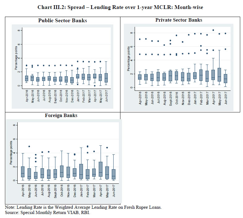 Bank-wise Analysis III.9 The distribution of monthly spreads of individual banks across bank groups during April 2016 – June 2017 did not show any clear pattern (Chart III.3). This was reflected in (i) large differences in the median spread charged by different banks; (ii) large divergence in the minimum and maximum spreads charged by individual banks across all bank groups; and (iii) excessively volatile spreads (as reflected by the length of the box) of some banks, particularly private sector and foreign banks. Spreads Charged – Select Individual Banks III.10 An analysis of spreads of 14 major individual banks (public, private and foreign) suggests that spreads charged on fresh rupee loans varied significantly across banks during the period (April 2016 to June 2017). Spreads charged widened in January 2017 in 12 out of 14 selected banks; the spread declined in the case of one bank and remained unchanged for another bank. Banks were slow to pass on the reduction in their MCLRs in January 2017 to their actual lending rates. Of the 12 banks whose spreads widened, six banks took up to six months to pass on the benefit of lower MCLRs to their lending rates; the remaining six banks passed on the benefit of their lower MCLRs, but only partially even after six months. This is intriguing as changes in MCLRs are expected to be passed on to at least fresh borrowers immediately (Chart III.4). III. Outstanding Rupee Loans6: Spreads Charged by Banks Analysis Based on Median Spreads III.11 An examination of monthly data on the median spread7 of bank groups suggests that public sector banks maintained a relatively steady spread of 159-178 bps during April 2016 to December 2016 (Chart III.5). However, the median MCLR declined by 65 bps in January 2017, which resulted in the median spread widening by around 58 bps to 228 bps in January 2017 (from 170 bps in December 2016). In subsequent months, the median spread charged by public sector banks declined gradually to 206 bps in June 2017, but it was above the level that prevailed in December 2016. III.12 The median spread charged by private sector banks peaked at 234 bps in January 2017 (from 219 bps in April 2016). However, the median spread declined sharply to 202 bps in June 2017 and was lower than the level that prevailed in December 2016. It is significant that the median spread of private sector banks remained consistently higher than that of public sector banks during the entire period April 2016 – May 2017, but was marginally lower in June 2017. III.13 The median spread charged by foreign banks was much lower than that by public and private sector banks. The median spread of foreign banks, which was 74 bps in April 2016, increased to 107 bps in January 2017, before declining to 86 bps in June 2017. The median spread of foreign banks during April 2016-June 2017 moved in a narrow range in comparison with that of public and private sector banks. III.14 The median spread for the banking industry as a whole widened significantly in January 2017 and remained elevated broadly at that level till May 2017 before declining sharply in June 2017; the spread was 166 bps in December 2016 and 176 bps in June 2017. III.15 On the whole, the spread of public sector banks widened significantly between April 2016 and June 2017 (Table III.2). The sharp reduction in the MCLRs by public sector banks in January 2017, which was reflected in the widening of the spread, was passed on to their lending rates only partly in subsequent months. Table III.2: Change in the Median Spread – Outstanding Rupee Loans
(Lending Rate over 1-year MCLR) | | (Basis points) | | Period | Public Sector Banks | Private Sector Banks | Foreign Banks | Scheduled Commercial Banks | | April-December 2016 | 11 | -1 | 31 | 13 | | January 2017 | 58 | 16 | 2 | 30 | | February - June 2017 | -23 | -32 | -21 | -20 | | April 2016 - June 2017 | 46 | -17 | 12 | 23 | Note: Lending Rate is the Weighted Average Lending Rate on Outstanding Rupee Loans.
Source: Special Monthly Return VIAB, RBI. | Distribution of Spreads - Temporal Variations III.16 Based on distribution of spreads across banks and over time, the following two points emerge. First, in comparison with spreads on fresh rupee loans, variations in spreads on outstanding rupee loans were relatively larger (Chart III.6). Second, of the three bank groups, spreads of foreign banks were more volatile in comparison with the two other bank groups. IV. Sector-wise Spread III.17 Spreads across sectors (i.e., sectoral WALR – median 1-year MCLR) need not be uniform due to idiosyncratic factors as reflected in credit risk and business strategy followed by banks. For instance, spreads are expected to be the lowest for those sectors where loans can be easily collateralised (e.g., mortgages and vehicle loans). The availability of subvention and mandated lending under priority sector norms also contribute to lower spreads (e.g., agriculture, low value residential housing loans). On the other hand, spreads are expected to be high in those sectors where there is a higher probability of default (e.g., large industry, infrastructure), or where transaction costs are relatively high and banks enjoy pricing power in the absence of alternative sources of financing (e.g., MSMEs). Spreads could be expected to be high in the case of credit card loans where credit is extended in the form of unsecured advances. Spreads across sectors have indeed varied (Table III.3). However, what is intriguing is the large extent of variation in spreads across sectors (110 bps to 307 bps in April 2016 and 106 bps to 322 bps in June 2017), excluding credit cards. | Table III.3: Spread – Lending Rate and 1-Year MCLR: Sector-wise | | (Basis points) | | Sector | April 2016 | December 2016 | January 2017 | June 2017 | | Agriculture | 128 | 171 | 226 | 225 | | Industry (Large) | 287 | 248 | 294 | 275 | | MSMEs | 284 | 288 | 319 | 322 | | Infrastructure | 281 | 263 | 332 | 306 | | Trade | 307 | 263 | 315 | 288 | | Professional Services | 230 | 234 | 270 | 238 | | Personal Housing | 110 | 80 | 134 | 106 | | Personal Vehicle | 220 | 209 | 256 | 234 | | Education | 297 | 280 | 316 | 300 | | Credit Card | 2891 | 2969 | 3045 | 3035 | Note: Lending Rate is the Weighted Average Lending Rate on Outstanding Rupee Loans.
Source: Special Monthly Return VIAB, RBI. | III.18 Spreads charged by banks widened significantly across sectors in January 2017 from their levels in December 2016. Although spreads declined by June 2017, they were still significantly higher than those prevailing in December 2016 for almost all the sectors. This corroborates the findings of the previous sections of weak transmission from the reduction in MCLRs to lending rates across sectors (Table III.3). V. Spreads Charged by Banks: Some Issues III.19 The issue of effective monetary transmission has been at the center-stage after deposit and lending interest rates were deregulated in the mid-1990s and the Reserve Bank started conducting monetary policy based on interest rates in the second half of the 1990s. The MCLR system, introduced in April 2016, was expected to improve transparency in setting interest rates and strengthen monetary transmission. The MCLR system differed from the base rate system in two major respects, viz., (i) the cost of funds for setting the interest rate was required to be based on marginal cost of funds (instead of marginal or average or a combination thereof under the base rate system); and (ii) the spread to be charged over the base rate was made less discretionary as it contained only two elements, viz., business strategy and credit risk (in the case of base rate, spreads included several elements such as tenor premia, allocable portion of operating costs and credit risk, among others). III.20 The experience with the spreads charged over MCLRs by banks, however, raises several concerns. First, although the spread to be charged by banks was expected to play a role only at the margin, it turned out to be the key element in the determination of the overall lending rates. Banks in general used the flexibility accorded to them arbitrarily, which is evident from (i) large variations in spreads charged across banks; (ii) too large spreads in some cases to be justified based on business strategy and credit risk profile of the borrowers; (iii) slow and incomplete pass-through from reduction in the MCLRs to lending rates even in the case of fresh rupee loans; (iv) increase in spreads charged by some banks at the same time when the MCLRs were reduced, ostensibly to partly compensate for the reduction in MCLRs; and (v) large variations in spreads charged over time. A special study conducted by the Study Group corroborates that banks adjusted the spreads arbitrarily in several ways (Box III.1). Box III.1: Spreads over MCLRs – A Study of Select Banks: Key Findings The Study Group conducted a special study with a view to ascertaining the practices followed by banks in India in fixing the spreads over MCLRs. The key findings that emerged from the study are set out below. -
Many banks indulged in arbitrary adjustment of spreads. The large reduction in MCLRs by some banks was partly offset by an increase in the spread in the form of business strategy premium. This happened in the case of housing loans and unsecured personal loans, among others. -
Some banks did not have a board approved policy for working out the components of the spread charged to a customer. -
In the case of some banks, there was no concept of a “spread” as envisaged in the extant Reserve Bank’s guidelines. Instead, it was only a balancing figure that resulted from the difference between the final rate calculated as per the bank’s own internal interest rate framework and the MCLR calculated by the bank. The pricing framework of some banks also had a provision for factoring in an “ALCO Strategy”, i.e., ALCO’s discretion to increase/decrease rates depending on the market conditions, competitive pressures and product penetration, among others. -
The credit risk premium applied was not individual customer specific, but it was computed on the basis of historically observed probability of default (PD) and loss given default (LGD) on the respective portfolio. -
One bank charged business strategy premium of 10 per cent for start ups, but the rationale was not documented. The same bank indicated that any spread charged over and above the credit spread was the business spread. -
One bank simply loaded a business strategy premium so as to match the MCLR with the existing base rate and the expected market rate. -
Strategy premium in the case of one bank was based on subjective parameters such as negative sector outlook and portfolio performance, concentration risk in the sector, NIM protection, other income/cross selling and market competition, among others. -
Some banks defined risk premium such that the variable component of the business strategy premium was added to the credit risk premium. This allowed them to vary the spread in a range of about 475 basis points for advances to various sectors. -
One bank mispriced credit risk as it had not assigned PD to different grades of its internal ratings. On the other hand, another bank charged a high credit risk spread, notwithstanding a low gross non-performing assets ratio (GNPA). Another bank did not have a unique credit risk spread for the same Credit Information Bureau of India Limited (CIBIL) score. -
One bank included a negative spread under business strategy due to market competition, which was in contravention to regulatory guidelines. -
Some banks applied liquidity premium in spread calculation despite MCLR being a tenor-linked benchmark. -
One bank applied business strategy premium across the portfolio without any discrimination across sectors/industries, which was more like an ‘adjusting factor’ than for any strategic differentiation. | III.21 As per the existing guidelines, the spread charged to an existing borrower under the MCLR cannot be increased except on account of deterioration in the credit risk profile of the customer. Any such decision regarding change in the spread on account of change in credit risk profile is required to be supported by a full-fledged risk profile review of the customer. The Study Group notes with concern that banks have not adhered to the Reserve Bank’s guidelines and have varied the spread charged to individual borrowers independent of any credit event. Further, as per extant guidelines, existing loans and credit limits linked to the Base Rate/BPLR are allowed to continue till repayment or renewal, as the case may be, provided that existing borrowers have the option to move to the MCLR linked loan at mutually acceptable terms. Some banks took advantage of this freedom and revised the spreads upwards at the time of conversion to keep the lending interest rate unchanged. III.22 The base rate and the MCLR systems suffer from a major flaw in that there is lack of transparency in the manner in which banks decide the spreads over the benchmark rates. What matters for the borrower is the actual lending rate charged. However, it is equally important for the borrower to know as to how the interest rate charged to him has been arrived at. This is all the more important when the lending interest rate contains different elements such as base rate/MCLR and the spread based on business strategy and credit risk and other elements (as in the case of the base rate). There have been often complaints from the borrowers about the lack of transparency in charging interest rates by banks, which is also corroborated by a special study of select banks conducted by the Study Group. In view of these reasons, the Study Group is of the view that there is a need for complete transparency about lending interest rates charged by banks. Recommendation III.23 The Study Group recommends that it should be made mandatory for banks to display prominently in each branch the base rate/MCLR (tenor-wise) and the weighted average lending rates on loans across sectors separately for loans linked to the base rate and the MCLR. The same information should also be hosted prominently on each bank’s website. The Reserve Bank could prescribe the format and the manner in which a minimum set of standardised data needs to be displayed in branches/hosted on banks’ websites. The Indian Banks’ Association (IBA), or any other agency considered appropriate by banks, could also disseminate bank-wise information on its website in the same manner in which each bank is required to disseminate information on its own website so as to facilitate easy comparison of lending rates across sectors and banks. The same system of dissemination of information on the benchmark and the weighted average lending rate could be followed under the external benchmark system recommended by the Study Group (see paras IV.43 - IV.45). VI. The Way Forward III.24 Based on the analysis in this and the previous chapters and a review of the practices followed by banks in computing base rates/MCLRs and charging spreads as revealed by the special study of select banks, the Study Group feels that the Reserve Bank’s approach, going forward, needs to keep in view the following factors. First, the experiences with the PLR, the BPLR, the base rate and the MCLR systems suggest that interest rate setting based on an internal benchmark is not transparent as banks find ways to work around. Second, the interest rate setting based on an internal benchmark such as MCLR is not in sync with the practices followed in the modern banking system. Third, for improving transmission and extending equal treatment to the existing and new borrowers, there is a need to make the liability side of banks’ balance sheet more responsive to policy rate changes. The Study Group feels that the liability side may not become adequately responsive to monetary policy impulses unless it is driven by the asset side, the aspect which is covered in the following chapter. ______________________________
Chapter IV
Exploring Market Rates as Benchmarks I. Introduction IV.1 The analysis in previous chapters underlined the limitations of internal benchmarks, viz., the base rate and the MCLR. Internal benchmarks have perpetuated rigidities on the liability side of banks’ balance sheet. These rigidities then feed into higher pricing on the asset side, i.e., lending rates, thereby impeding monetary policy transmission. Both the base rate and the MCLR systems, by overemphasising the cost of funds as the prime mover of monetary policy transmission, have not worked as expected. For effective monetary policy transmission, it is important that lending interest rates are flexible and set in a transparent manner. IV.2 In the modern day financial systems, external benchmarks occupy the position of a central anchor around which the pricing of financial products evolves. Estimated outstanding value of financial contracts using LIBOR as the reference benchmark in the world is pegged at about USD 350 trillion (Debelle, 2017). While more than 90 per cent of the interest rate derivatives use LIBOR as the reference benchmark, corporate loans (30-50 per cent), retail mortgages (15 per cent), floating rate bonds (about 84 per cent) and securitised products (about 24 per cent) also use LIBOR [Alternative Reference Rates Committee (ARRC), 2016]. Financial systems around the world have devoted considerable resources for strengthening and refining market benchmarks in recent years, particularly after the LIBOR fixing episode surfaced. IV.3 In this Chapter, various market-based benchmarks are explored with a view to assessing their suitability for the credit market in India in light of recent international developments. Linking lending interest rates to an external benchmark could play a critical role in introducing necessary flexibility on the liability side of banks. II. Recent Global Developments and Initiatives on External Benchmarks IV.4 Inter-bank offered rates (IBORs) such as London Inter-bank Offered Rate (LIBOR), Euro Inter-bank Offered Rate (EURIBOR) and Tokyo Inter-bank Offered Rate (TIBOR) have been used extensively as benchmarks in both the credit and derivatives markets in major advanced economies (Table IV.1). | Table IV.1: Use of IBORs as Benchmarks | | (Per cent of total volumes) | | Segment | US Dollar
(LIBOR) | Euro
(EURIBOR) | Pound Sterling
(LIBOR) | Japanese Yen
(TIBOR) | Swiss Franc
(LIBOR) | | Credit Market | | Syndicated Loans | 97 | 90 | 100 | High | 50-70 | | Business Loans | 30-50 | 60 | 68 | 20 | 40-60 | | Commercial Mortgages | 30-50 | 60 | Low | NA | 15-25 | | Retail Mortgages | 15 | 28 | 1-2 | NA | 10-20 | | Consumer Loans | Low | Low | Low | NA | NA | | Derivatives Market | | Over the Counter (OTC) | 65 | High | 62 | 58.3 | 98-100 | | Exchange Traded | 92 | 100 | 98.5 | 100 | 100 | | Source: Financial Stability Board (Reforming Major Interest Rate Benchmarks; July 22, 2014). | IV.5 The recent international debate on search for alternative benchmarks was triggered by the unexpected behavior of IBORs under extreme stressed conditions after the global financial crisis and the LIBOR scandal of 2012. After the announcement of the findings of a probe against Barclays in June 2012, the final report of the Wheatley Review of LIBOR, submitted in September 2012, recommended ways to reform the framework for fixing and governing LIBOR. Strikingly, the report highlighted that “…despite the loss of credibility that LIBOR has suffered recently, there has been no noticeable decline in the use of LIBOR by market participants….(for LIBOR) there is no immediately obvious alternative”. In a recent speech, however, Andrew Bailey, Chief Executive of the Financial Conduct Authority (FCA) in the UK (which is the administrator of LIBOR) expressed major concerns about the future of LIBOR. The absence of underlying deep markets for transaction-based LIBOR has posed challenges for the panel banks submitting quotes, who often have to apply expert judgment (considered acceptable under the waterfall approach as elaborated later). While the panel banks are uncomfortable to continue with the current system, they have voluntarily agreed to sustain LIBOR until end-2021. This timeframe allows enough time to jurisdictions to look for alternative robust benchmarks. IV.6 Anticipating the challenges ahead, the Global Financial Market Association (GFMA) finalised in November 2012 a set of principles for financial benchmarks (known as GFMA principles) highlighting the need for development of international standards to govern financial benchmarks. In response, the International Organisation of Securities Commission (IOSCO) developed the IOSCO Principles for financial benchmarks in its final report submitted in July 2013 (Annex IV.1). IV.7 Recognising the integrity of reference rates as a source of financial system vulnerability, the G20 tasked the Financial Stability Board (FSB) to undertake a fundamental review of major interest rate benchmarks and propose reforms. The FSB submitted its report titled “Reforming Major Interest Rate Benchmarks” in July 2014. An Interim report on the implementation of the recommendations in terms of progress in reforming major interest rate benchmarks was submitted by the FSB in July 2015, followed by an update in July 2016. In the US, the Federal Reserve convened the Alternative Reference Rates Committee (ARRC) in November 2014 with specific terms of reference. The interim report was submitted by the ARRC in May 2016. IV.8 In Australia, the Australian Securities and Investments Commission (ASIC) submitted a report in July 2015 on financial benchmarks with recommendations to address potential manipulation of financial benchmarks and related conduct issues. The European Money Market Institute produced a consultative paper on enhancements to the Euro Overnight Index Average (EONIA) benchmark in August 2016. In the Euro area, a new working group was constituted on September 21, 2017 to identify and facilitate adoption of a ‘risk-free overnight rate’ as an alternative to current benchmarks. The ECB announced on the same day that it will publish a new unsecured overnight interest rate by 2020, complementing existing benchmark rates produced by the private sector. In Japan, a study group submitted a report on the identification of a Japanese Yen risk free rate in December 2016, which was preceded by another report submitted in March 2016 aimed at public consultations and seeking comments from a wide range of interested parties. In the UK, the working group on sterling risk-free reference rates submitted its report in May 2016. The Bank of England published a consultation paper on the reform of SONIA in October 2016, followed by an update in February 2017. The BIS published a report in March 2013 setting out a central banking perspective on better reference rate practices. IV.9 The recommendations of the above referred reports broadly cover country-specific reviews aimed at smoother transitions to more appropriate benchmarks. From the standpoint of what may be relevant to the credit market in India, the following important points emerge from a review of these reports: a) There is a global trend to move away from the earlier “quote” based IBOR system to the “transaction” based IBOR+ (or enhanced IBOR) systems. b) From the standpoint of the credit market, the reference benchmark rate must relate to the cost of funds of banks at the margin, which need not include only unsecured inter-bank borrowing, but may also include bank certificates of deposit (CDs) and bonds. Thus, it is now believed that the most appropriate reflection of the marginal cost of unsecured wholesale funding for banks is not only the inter-bank market, but also a wide variety of unsecured borrowing instruments. c) In the absence of adequate transaction level data, a “waterfall” or “hierarchy approach” could be followed: (i) the first level requirement is actual transaction-based data; (ii) if actual transaction data are not available, then at the second level committed/executable quotes (i.e., orders placed at arm’s length by buyers and sellers) could be used; (iii) in the absence of such committed quotes, transaction data from comparable wholesale funding markets could be used; and (iv) in the absence of all three preceding levels, use of expert judgment is advised, which should nevertheless be exercised only on very rare occasions. In a deep market that sets the benchmark, first two levels should ideally not leave any scope for any recourse to the latter two levels. d) An IBOR+ that may involve some bank credit risk (reflecting essentially bank funding costs at the margin) is suitable for the credit market, while a near risk free benchmark is more suitable for derivative products (which currently use IBORs). This is because derivative contracts express trading on interest rate expectations. As such, reference rates for derivative transactions need not incorporate bank credit risk component. e) Most reference rate activity is concentrated at shorter tenors, up to three months. The Wheatley Review highlighted that of the large number of published LIBOR benchmarks, very few could be supported by actual transaction data. Also, not many of them were possibly being heavily used by market participants. It was of the view that on implementation of its recommendations in full, LIBOR benchmarks (covering different tenors and currencies) should decline from 150 to 20. f) Private contracts must reflect private choices on the use of any preferred benchmark. However, the governments, especially regulators for banks and financial markets, need to ensure that market-based benchmarks meet the best global standards such as the IOSCO principles. The final report of the IOSCO has set out 19 principles covering governance and accountability standards for the benchmark administrator to protect the integrity of the benchmark determination process, quality of the benchmarks, oversight mechanisms, quality of the methodology, transparency, and the code of conduct for the submitters (Annex IV.1). III. Desirable Properties of an Ideal Benchmark IV.10 With the financial systems becoming large and increasingly complex over time, no single benchmark could possibly meet the requirements of all market participants. Country experiences, market feedback, and analytical reviews presented in various reports nevertheless suggest the following desirable properties that an ideal benchmark should possess. Robustness and Reliability IV.11 The benchmark must be based on actual transactions, and should emerge from a deep and liquid market. An often quoted axiom in this context is: “a benchmark is as robust as its underlying market”. In a deep and liquid market, no single market player can move the rate. If a benchmark reflects the interaction of demand and supply in a deep and liquid market, then it can anchor the process of efficient allocation of capital and risk, which is so critical for an efficient financial system. IV.12 Preventing any scope for manipulation of the benchmark is important to establish its integrity and reliability. All stakeholders, ranging from regulators and benchmark administrators to banks, dealers, financial institutions and wealth managers, have a responsibility to contribute to fostering the integrity of the benchmark. Market manipulation is now treated as a criminal offence in many countries, punishable by imprisonment of a maximum of seven years (in the UK), minimum four years (in the European Union) and maximum seven years (in Singapore). Benchmark manipulation can benefit the trading positions of individual entities and, therefore, there may be natural incentives to do so. The governance structure and the legal environment must create strong disincentives for anyone to manipulate a benchmark. IV.13 The benchmark should also be resilient in stressed conditions. That is, the underlying market should be able to produce the benchmark even during periods of extreme market stress. Transparent Methodology IV.14 The methodology for calculating the benchmark should be simple and easy to understand. In view of the fact that IBOR+ type benchmarks follow the waterfall approach (as explained above), transparency about the methodology, techniques used for interpolation and extrapolation, and standardisation of parameters used in the construction of a benchmark become critical. The market oversight process, as a critical component of the governance structure, can also help in enhancing the reliability of the benchmark among market participants. Stability IV.15 A volatile benchmark could alter pricing decisions in terms of seeking an extra premium for uncertainty. Some reports reviewed (as referred to earlier), therefore, suggest the use of smoothing techniques to limit volatility, particularly for longer tenor. Term Structure IV.16 A benchmark should have a term curve covering the full spectrum of maturities in the money market. This enables pricing of products for varied tenors. Most transaction-based benchmarks globally do not meet this requirement. Concerns on liquidity beyond one month and three months in most underlying markets have necessitated use of the waterfall approach, as alluded to before. Even the advanced economies (AEs) are struggling to have IBOR+ term structures beyond 3 to 6 months tenor. Relationship with Banks’ Marginal Cost of Funds IV.17 From the standpoint of the credit market, it is important that the benchmark represents the banks’ marginal cost of funds. The LIBOR, which continues to be the prime benchmark in the global credit market, essentially refers to the cost of banks’ borrowings from the unsecured market, i.e., the market where any bank could meet the marginal funding requirements. An unsecured inter-bank market where banks would seek marginal funds, before coming to the lender of the last resort for liquidity, should be a close approximation of banks’ marginal funding cost. The IBOR+ approach highlights that in the event of lack of a term unsecured market, access to broader comparable markets such as CDs and corporate bonds could be used under the waterfall approach. Unlike the Indian MCLR, nowhere else the emphasis is on marginal cost of deposits. High Correlation with the Policy Rate IV.18 This is not a standard requirement of an external benchmark. However, given the focus of the Study Group on examining external benchmarks from the standpoint of strengthening transmission of monetary policy, high correlation with the policy rate was considered an additional desirable property in the Indian context. IV. Benchmark for the Credit Market in India: An Assessment of Possible Candidates IV.19 The Study Group examined the following instruments from the standpoint of their suitability as a benchmark for use in the credit market in India. The pros and cons of possible candidates as a benchmark for the credit market are detailed below. The main points are summed up in Annex IV.2a and IV.2b. Weighted Average Call Money Rate (WACR) IV.20 The weighted average call money rate (WACR) being the operating target of monetary policy tracks closely the policy repo rate. Hence, the transmission from the call rate to the credit market should be quick and strong. The methodology for computing the rate is also transparent. However, the WACR as a benchmark also has several disadvantages. First, it is a part of the operating framework of monetary policy. Hence, it may constrain future changes in the operating framework. The Report of the Expert Committee to Revise and Strengthen the Monetary Policy Framework in India (Chairman: Dr. Urjit R. Patel) had recommended, inter alia, that the 14-day term repo rate may become the operating target in future, replacing the WACR. Second, volumes in this market have declined in the recent period. The low market depth makes the rate susceptible to significant gyrations under extreme liquidity conditions. Also, reported transactions by some market participants below the market rate distort the WACR. Third, since there is no adequate depth in the call money market, banks may be able to raise only limited funds from the unsecured call money market. Fourth, being an overnight rate, the call money rate has no term structure. Fifth, call rates at times could also come under pressure and become volatile. Greater and repeated recourse to this market by banks for meeting higher funding needs could take the WACR closer to the ceiling of the liquidity adjustment facility (LAF) corridor and away from the repo rate. Likewise, in large surplus liquidity conditions, this rate could occasionally drop below the lower bound of the corridor. For instance, the WACR has been trading with a softening bias relative to the repo rate under the influence of persistent liquidity surplus post demonetisation. On some days, the WACR was even below the reverse repo rate. The new Basel III liquidity coverage ratio (LCR) regime also impacted spreads of WACR over the repo rate in the past (Pattanaik et al., 2017). Any future changes in regulations on liquidity risk for banks could impact the WACR. Overnight CBLO Rate and Market Repo Rate IV.21 The collateralised borrowing and lending obligation (CBLO) is the largest overnight segment and has wider participation base on both the lending and borrowing sides. The methodology for computation of the CBLO rate is transparent. It is also closely aligned with the policy repo rate. These features of the CBLO rate are also shared by the market repo rate. Both the rates are also linked to banks’ cost of funds at the margin. There are, however, some drawbacks of both these segments. First, the rate and volumes in the CBLO market drop on every reporting Friday. It is susceptible to pressure on rates from mutual funds as they dominate the market on the lending side. Similarly, the rate and volume drop on non-reporting Fridays in the market repo segment. Variability within a fortnight unrelated to the repo rate (because of market microstructure and regulatory norms) could spill over to the entire credit market, if used as a benchmark. Second, both these markets are collateralised. As such, rates in these segments could also at times reflect the impact of collateral constraints. G-sec/ T-bill Yields, FBIL-TB Rate IV.22 Yields on Government Security (G-sec) and Treasury Bills1 (T-Bills) are transparent, which emerge from the competitive biddings (primary market) and screen-based trading on the negotiated dealing system - order matching (NDS-OM) trading platform (secondary market). G-sec/T-Bill yields move with the policy repo rate. The term structure in these segments also exists, although volumes are low. However, the use of G-sec/T-Bill rates as a benchmark also raises some concerns. First, yields on government papers (whether T-Bills or dated G-sec) are generally not favoured as they are too sensitive to changes in fiscal policies. Second, such rates, if used as benchmarks, can constrain fiscal/debt management/cash management policies of the government. Third, after the sovereign debt crisis, yields on government papers have become susceptible to global spillovers. EMEs with exposure to portfolio debt flows also experienced the risk-on risk-off cycles impacting domestic yields. Spillovers induced market stress may alter yields dramatically, unrelated to the prevailing monetary policy stance. A benchmark based on government papers would not be resilient under stressed conditions. Fourth, if the yield on government paper is used as a benchmark in the credit market, the impact of fiscal policies and global spillovers can get transmitted directly to the credit market. Fifth, the marginal cost of funds raised by banks need not always exhibit a strong relationship with cost of funds raised by the government. Sixth, the G-sec market is also not deep enough to prevent the scope for manipulation by market participants. Lack of liquidity may lead to price changes even when a single market player takes/shifts large positions. IV.23 FBIL-TB rate as a benchmark raises the same concerns as T-Bills and G-sec yields. MIBOR and MIFOR IV.24 Mumbai Interbank Outright Rate (MIBOR) is based on overnight call money market transactions during the first market hour (i.e., 9 AM to 10 AM). Hence, limitations of WACR also apply to MIBOR. Mumbai Inter-bank Forward Offer Rate (MIFOR) is a poll-based rate and as such it is susceptible to manipulation. MIBOR and MIFOR are akin to (near) risk free benchmark rates (RFRs). Internationally, it is recognised that such rates are better suited for derivative transactions than for the credit market. Globally, RFRs such as overnight bank funding rate (OBFR) in the US, euro overnight index average (EONIA) in the Euro-area, Tokyo Overnight Average Rate (TONAR) in Japan, and sterling overnight index average (SONIA) in the UK are essentially overnight (near) risk free rates, which are being increasingly used/explored as alternatives to the LIBOR in derivative transactions. While MIBOR is already being used as a reference rate in the overnight index swap (OIS) market in India, MIFOR is used in the interest rate swap (IRS) market. If MIBOR/MIFOR is used as a benchmark in the credit market, it will create incentives for market participants to manipulate the underlying benchmark rate in one segment to take advantage in the other. Keeping in view recent international developments, the Study Group is of the view that MIBOR and MIFOR are not appropriate benchmarks for the credit market as these rates could be susceptible to manipulation. Overnight Index Swap (OIS) Rate IV.25 The OIS refers to the exchange of overnight floating interest rate with fixed interest rate. The OIS market in India has a term structure up to 10 years, but most segments are not liquid; the market participation is highly concentrated; and the price discovery process has been such that it would require high analytical skills and market specific knowledge to decipher the OIS rates. The fixed rate that market participants exchange for the floating MIBOR may vary over time because of changing interest rate expectations, including monetary policy expectations, which need not always materialise. As such, the OIS rate would not be appropriate for the credit market, especially for retail loans. Loan contracts need to be based on benchmarks that are not driven excessively by interest rate expectations. Certificates of Deposit (CD) Rate and FBIL-CD Rates IV.26 The Study Group is of the view that the CD rate satisfies many of the desirable properties of an ideal benchmark for the credit market. First, these rates are based on actual transactions. Interest rates from both the primary and secondary markets are available. About 30 per cent of the total CDs issued by banks are held by other banks, and as a result it is partly inter-bank in nature. For this reason, it also contains bank credit risk, which is relevant for pricing products in the credit market. CDs could be viewed as a proxy for bank funding cost. Second, it already has a term curve starting from 14-days to nine months. For these reasons, CD rates are akin to IBOR+ which many advanced countries are trying to develop as a replacement of poll-based IBORs. Third, foreign portfolio investors (FPIs) are not permitted to invest in CDs. Therefore, CD rates are also not susceptible to global spillovers directly. Fourth, CD rates exhibit high degree of transmission during both the tightening and easing phases of monetary policy cycles. IV.27 The Study Group, however, recognised several limitations of CD rates. First, the reference rate of Thomson Reuters is based on polls. The FBIL CD rates – though transaction-based and the methodology is to an extent in sync with the waterfall approach – are yet to be tested for robustness. Also, CD rates are based on bilaterally settled trades between parties, rather than order matching anonymous trading platform (see Annex IV.3 for FBIL-CD methodology). For this reason, the second level of waterfall approach (executable bids) is not available. Second, volumes are too low in the CD market as not many large banks issue CDs. Lack of market depth will not be able to insulate the rates from motivated large market transactions, both on the issuing and investment sides. Third, CD rates remain highly sensitive to liquidity conditions. 14-day Term Repo Rate IV.28 Since the first auction of term repos under the revised liquidity management framework about three years ago (September 2014), a time series of 14-day term repo rates (in terms of both cut-offs for every auction and the weighted average rates) has emerged through regular committed auctions. These rates, which are available four times in a fortnight, are close to the policy repo rate, transparent and reliable. However, the 14-day term repo rate as a benchmark has some drawbacks: (a) these rates are not available every day; (b) the intended development of the inter-bank term money market has not materialised as yet; and (c) in persistent surplus liquidity conditions, it may cease to be an effective rate. In surplus liquidity conditions, the term reverse repo rate becomes the effective rate. For these reasons, the 14-day term repo is not appropriate for an external benchmark. Policy Repo Rate IV.29 A major point in favour of the policy repo rate as a benchmark is that it is robust and reliable as it is decided by the monetary policy committee (MPC) keeping in view the macroeconomic conditions. It is also transparent, simple and easy to understand by the general public. Another major advantage is that the transmission from the repo rate to lending rates will be direct, quick and strong. However, the policy repo rate as a benchmark also raises some issues. An important point that goes against the use of policy interest rate as the benchmark is that it might constrain future changes in the monetary policy framework. Going by the past experience, changes in the monetary policy framework in future cannot be ruled out. Should there be any major change in the monetary policy framework with a bearing on the repo rate, it could raise concerns about the stability of the benchmark. In some situations, the policy repo rate may also cease to be an effective policy rate. For instance, after the ‘taper tantrum’ in May 2013, the marginal standing facility (MSF) rate became the effective policy rate. IV.30 If a benchmark has to serve its intended objectives, it should be possible for banks to access funding at the benchmark rate from the market at the margin, which would automatically involve some credit risk in the benchmark. However, individual banks cannot access funding from the Reserve Bank at the repo rate beyond the limit (i.e., 0.25 per cent of their net demand and time liabilities). IV.31 After carefully analysing the pros and cons of each possible candidate, the Study Group is of the view that certain market rates such as MIBOR, MIFOR, OIS rate and the 14-day term repo rate are not suitable as a benchmark for the credit market in India for the reasons already alluded to. The CBLO and market repo rates were also not found suitable as interest rates in these segments often spike. As a result, these two rates are much more volatile than other money market rates (Table IV.4). The WACR is rejected on two main grounds. First, volumes have declined/stagnated in the overnight call money market in the recent period. Second, it is a part of the operating framework of monetary policy. Therefore, if any element of the monetary policy/operating framework is to be considered as a benchmark, then the repo rate is certainly a better choice. Also, international as well as Indian experiences suggest that changes in the policy framework, in general, are far less frequent than those in the operating framework. As the monetary policy framework is now contained in the amended Reserve Bank of India Act, 1934, any changes in the policy framework will require legislative amendments. However, the operating framework could be changed by the Reserve Bank any time. G-sec yields are highly sensitive to fiscal policy changes and global spillovers. As such, they would not be an appropriate anchor for the credit market from the standpoint of transmission of monetary policy impulses. IV.32 A careful process of elimination enabled the Study Group to narrow down its choices to essentially two market-based candidates, viz., the T-Bill rate and the CD rate; and the Reserve Bank’s policy repo rate. The first two rates were further assessed on three criteria, viz., (i) correlation with the policy repo rate; (ii) stability; and (iii) liquidity. Monetary policy transmission has been strong in both these instruments. A cumulative 200 bps cut in the repo rate since January 2015 has been by and large transmitted to these rates (Table IV.2). The transmission was robust in the previous easing cycle of monetary policy as well, suggesting that this transmission may not alter significantly even if liquidity conditions return to neutrality (ex ante). | Table IV.2: Monetary Policy Transmission: Different Phases of the Monetary Policy Cycle | | (Variation in basis points) | | Policy Cycle | Repo Rate | WACR | CBLO | Market Repo | 91-day T-Bills | 3-month CD | MIBOR | 3-month MIFOR | 3-month OIS | 1-year OIS | 1-year G-sec | 5-year G-sec | 10-year G-sec | | Easing Phase | | April 2012 - June 2013 | -125 | -165 | -150 | -136 | -106 | -165 | -179 | -193 | -80 | -37 | -37 | -63 | -90 | | Tightening | | July 2013 - December 2014 | 75 | 118 | 150 | 127 | 80 | 43 | 124 | 148 | 53 | 20 | 71 | 17 | 32 | | Easing | | Since January 2015* | -200 | -225 | -252 | -249 | -222 | -240 | -235 | -266 | -210 | -150 | -207 | -140 | -126 | | *: Up to August 2017. | IV.33 The T-Bill rate and the CD rate are also highly correlated (and statistically significant) with the policy repo rate (Table IV.3). | Table IV.3: Correlation Coefficients – Policy Repo Rate with Other Rates | | | WACR | CBLO | Market Repo | 3M-CD | MIBOR | 3-month MIFOR | 6- month MIFOR | 91-TB | 1-yr G-sec | 5-yr G-sec | 10-yr G-sec | | Lag 0 | 0.82 | 0.74 | 0.81 | 0.83 | 0.81 | 0.69 | 0.59 | 0.80 | 0.77 | 0.82 | 0.84 | | | (0.00) | (0.00) | (0.00) | (0.00) | (0.00) | (0.00) | (0.00) | (0.00) | (0.00) | (0.00) | (0.00) | | Lag 1 | 0.82 | 0.74 | 0.81 | 0.82 | 0.81 | 0.69 | 0.59 | 0.80 | 0.77 | 0.82 | 0.84 | | | (0.00) | (0.00) | (0.00) | (0.00) | (0.00) | (0.00) | (0.00) | (0.00) | (0.00) | (0.00) | (0.00) | | Lag 2 | 0.81 | 0.74 | 0.80 | 0.82 | 0.81 | 0.69 | 0.59 | 0.80 | 0.77 | 0.82 | 0.84 | | | (0.00) | (0.00) | (0.00) | (0.00) | (0.00) | (0.00) | (0.00) | (0.00) | (0.00) | (0.00) | (0.00) | | Lag 3 | 0.81 | 0.73 | 0.80 | 0.82 | 0.81 | 0.69 | 0.59 | 0.80 | 0.77 | 0.82 | 0.84 | | | (0.00) | (0.00) | (0.00) | (0.00) | (0.00) | (0.00) | (0.00) | (0.00) | (0.00) | (0.00) | (0.00) | Notes: 1. Figures in parentheses are p-values.
2. Estimation done on daily data from April 2012 to August 2017. | IV.34 Volatility of the T-Bill rate and the CD rate was assessed in terms of measures of standard deviation and coefficient of variation. Both the CD and T-Bill rates were among the least volatile rates in 2017 (Table IV.4). | Table IV.4: Interest Rate Volatility | | Year | WACR | CBLO | Market Repo | 91-day Treasury | 3-Month CD | MIBOR | 3-month MIFOR | 6-month MIFOR | 1-yr Govt. securities | 5-yr Govt. securities | 10-yr Govt. securities | | Average | | 2012 | 8.33 | 7.98 | 8.13 | 8.36 | 9.22 | 8.38 | 7.79 | 7.35 | 8.06 | 8.24 | 8.26 | | 2013 | 8.27 | 7.99 | 8.22 | 8.57 | 9.02 | 8.35 | 8.41 | 8.03 | 8.43 | 8.24 | 8.12 | | 2014 | 8.10 | 8.17 | 8.22 | 8.61 | 8.83 | 8.26 | 8.69 | 8.61 | 8.54 | 8.59 | 8.57 | | 2015 | 7.22 | 7.25 | 7.27 | 7.64 | 7.85 | 7.37 | 7.58 | 7.63 | 7.66 | 7.83 | 7.76 | | 2016 | 6.43 | 6.39 | 6.46 | 6.68 | 7.02 | 6.57 | 6.90 | 7.06 | 6.88 | 7.17 | 7.21 | | 2017* | 6.01 | 5.97 | 5.97 | 6.13 | 6.31 | 6.20 | 6.17 | 6.27 | 6.38 | 6.68 | 6.64 | | Standard Deviation | | 2012 | 0.51 | 0.87 | 0.63 | 0.29 | 0.84 | 0.48 | 0.76 | 0.54 | 0.09 | 0.15 | 0.16 | | 2013 | 1.03 | 1.31 | 1.08 | 1.15 | 0.97 | 1.03 | 1.12 | 1.04 | 0.94 | 0.58 | 0.54 | | 2014 | 0.36 | 0.47 | 0.37 | 0.24 | 0.43 | 0.40 | 0.48 | 0.43 | 0.21 | 0.29 | 0.29 | | 2015 | 0.46 | 0.43 | 0.62 | 0.43 | 0.51 | 0.41 | 0.57 | 0.39 | 0.34 | 0.13 | 0.09 | | 2016 | 0.25 | 0.36 | 0.27 | 0.39 | 0.68 | 0.27 | 0.84 | 0.66 | 0.34 | 0.44 | 0.46 | | 2017* | 0.08 | 0.27 | 0.28 | 0.15 | 0.12 | 0.12 | 0.19 | 0.21 | 0.11 | 0.17 | 0.20 | | Coefficient of Variation | | 2012 | 6.07 | 10.87 | 7.70 | 3.47 | 9.12 | 5.76 | 9.79 | 7.38 | 1.11 | 1.81 | 1.94 | | 2013 | 12.41 | 16.36 | 13.17 | 13.37 | 10.79 | 12.38 | 13.34 | 12.96 | 11.17 | 7.02 | 6.63 | | 2014 | 4.50 | 5.76 | 4.51 | 2.76 | 4.87 | 4.83 | 5.55 | 5.03 | 2.43 | 3.41 | 3.33 | | 2015 | 6.40 | 5.97 | 8.60 | 5.64 | 6.53 | 5.51 | 7.49 | 5.16 | 4.46 | 1.61 | 1.13 | | 2016 | 3.94 | 5.56 | 4.22 | 5.82 | 9.69 | 4.09 | 12.13 | 9.33 | 5.01 | 6.20 | 6.34 | | 2017* | 1.30 | 4.50 | 4.71 | 2.37 | 1.84 | 2.00 | 3.06 | 3.40 | 1.70 | 2.53 | 2.97 | WACR: Weighted Average Call Rate; CBLO: Collateralised Borrowing and Lending Obligations.
*: Based on daily data up to August 2017. | IV.35 For assessing the market depth, daily average volumes in each segment was normalised by bank deposits (the core source of funding for banks). However, of all segments, the CD and T-Bills segments were the least liquid (Table IV.5). | Table IV. 5: Volumes: Select Markets | | Item | Overnight Call Money Market | CBLO | Market Repo | 91-TB
(outright market) | CDs | OIS | G-sec
(outright market) | | Volumes (Rs. billion) | 148.5 | 614.5 | 276.2 | 19.5 | 52.8 | 84.6 | 340.8 | | As per cent of Bank Deposits | 0.159 | 0.659 | 0.296 | 0.021 | 0.057 | 0.091 | 0.365 | | Note: Pre-demonetisation period (average daily trading volumes in 2015-16) is used here. | IV.36 The analysis in this section suggests that the T-Bill rate and the CD rate are highly correlated with the policy repo rate and these rates are also among the least volatile rates. However, the T-Bill and CD markets are too thin. Of the two instruments, the T-Bill market is less susceptible to manipulation. This is because unlike the CD market, where rates are based on bilateral trades, T-Bill market transactions are based on the rates from both bilateral trades and an order matching anonymous platform2 (see Annex IV.4 for the FBIL methodology). Although inadequate liquidity in both the T-bill and CD segments is an issue, the scope for manipulation could be addressed by putting in place appropriate governance and accountability standards on the lines of IOSCO principles. IV.37 After a detailed analysis of the MCLR system as also the pros and cons of all possible candidates for an external benchmark, the Study Group had to make one of the following three choices for its recommendation: (i) continue with the MCLR as an internal benchmark with refinements as recommended by the Study Group; (ii) phase out the MCLR as an internal benchmark in a time-bound manner and let the external benchmark emerge as a market-driven process; and (iii) suggest the T-Bill rate, the CD rate and the policy repo rate as external benchmarks and the Reserve Bank could take a final view on an external benchmark after getting feedback from all stakeholders. IV.38 The first option, i.e., to continue with the MCLR system was not considered appropriate because of its opaqueness, which has undermined the integrity of the rate setting process and impeded monetary transmission. As alluded to earlier, interest rates based on a formula such as the MCLR is not the international best practice. IV.39 The second option, i.e., to phase out the MCLR in a time-bound manner and let the external benchmark emerge in a market-led process, was also not considered appropriate. The Study Group is of the view that it would be ideal if the external benchmark emerges in a market driven process. External benchmarks in India were allowed way back in 2000. However, there has not been much forward movement. Given the current depth of money markets in India, an external benchmark may not emerge in a time frame desirable for phasing out the MCLR. There is also a risk that multiple benchmarks emerge that may be applied differently across customers and sectors, which could be disorderly. The Study Group, therefore, is of the view that the development of an external benchmark in an orderly manner would need guidance from the Reserve Bank. IV.40 There is no one view as to what should be the role of central banks in reference rate processes. It varies across countries depending on institutional arrangements and other factors, especially the state of the development of the financial market. There are many cases where benchmarks have been driven by markets and central banks did not play any specific role in rate setting or oversight such as LIBOR and EURIBOR. However, more recently, several central banks (such as South African Reserve Bank, Hong Kong Monetary Authority, and Sveriges Riksbank) have been formally involved in reviews of rate setting processes, viz., for reference rates based on the unsecured inter-bank market. Central banks have also directly participated in the production of other reference rates to support market development. For instance, the Swiss National Bank developed the Swiss Reference Rate and related calculation methodology jointly with the Swiss Stock Exchange (SSE) to aid the development of repo markets. Similarly, in response to industry requests to support the development of repo markets, the Bank of Japan started the production of the Tokyo Repo Rate in 2007, before handing over production to the Japan Securities Dealers Association in 2012 (BIS, 2013). IV.41 In the absence of a market-led approach to adoption of a relevant benchmark in the credit market in India – possibly due to the lack of enough market depth to set a market-based reliable benchmark – the Study Group recognises that the Reserve Bank would need to play an active role in producing the benchmark, especially for the credit market, that it feels could best serve the interests of the banking system and the macro economy. This will be necessary for establishing the credibility and integrity of the benchmark. In this context, the observation by the Expert Committee to Revise and Strengthen the Monetary Policy Framework, 2014 (Chairman: Dr. Urjit R. Patel) is very relevant: “…it is necessary to develop a culture of establishing external benchmarks for setting interest rates based on which financial products can be priced. Ideally, these benchmarks should emerge from market practices. However, the Committee is of the view that the Reserve Bank could explore whether it can play a more active supportive role in its emergence”. IV.42 Keeping in view the above mentioned considerations, the Study Group is of the view that it will be desirable to move to an external benchmark. Of all the possible candidates considered, the T-Bill rate, the CD rate and the Reserve Bank’s repo rate are more suited to serve the role of an external benchmark. A final choice of a benchmark could be made by the Reserve Bank after wider public debate and getting feedback from all stakeholders. Recommendation IV.43 An evaluation of 13 possible candidates [weighted average call rate (WACR), collateralised borrowing and lending obligation (CBLO) rate, market repo rate, 14-day term repo rate, G-sec yields, T-Bill rate, certificates of deposit (CD) rate, Mumbai inter-bank outright rate (MIBOR), Mumbai inter-bank forward offer rate (MIFOR), overnight index swap (OIS) rate, Financial Benchmark India Ltd. (FBIL) CD rates, FBIL T-Bill rates and the Reserve Bank’s policy repo rate)] suggests that no instrument in India meets all the requirements of an ideal benchmark. Each instrument has certain advantages as also limitations. After carefully analysing the pros and cons of 13 possible candidates as a benchmark, the Study Group narrowed down its choice to three rates, viz., a risk-free curve involving T-Bill rates, the CD rates and the Reserve Bank’s policy repo rate. The T-Bill rate and the CD rate3 were further assessed on three parameters, viz., (i) correlation with the policy rate; (ii) stability; and (iii) liquidity. The Study Group is of the view that the T-Bill rate, the CD rate and the Reserve Bank’s policy repo rate are better suited than other interest rates to serve the role of an external benchmark. IV.44 The T-bill rates are risk free and also transparent. They also have a reliable term money market curve. CD rates relate to the credit market directly in the sense that banks could meet their marginal requirement of funds from this market. CDs also have a reliable term money market curve. Unlike the T-Bill market where the money market term curve is available up to 12 months, in the CD market, the term curve is generally up to six months (and up to 9 months occasionally). The main challenge in using either T-bill rates or CD rates as the benchmark is that the current level of market depth in the T-Bill and CD markets can make such benchmarks potentially susceptible to manipulation. Also, T-Bill rates may at times reflect fiscal risks which will automatically get transmitted to the credit market when used as a benchmark. CD rates also have their own limitations - high sensitivity to liquidity conditions, credit cycles, and seasonality. Liquidity in the CD market is inadequate because there are no large and frequent issuances by a sufficient number of highly rated banks. The Reserve Bank’s policy repo rate has the primary advantage that it is robust, reliable, transparent and easy to understand. It reflects the appropriate rate for the economy at any point in time based on the MPC’s assessment of macroeconomic conditions and the outlook. With the repo rate as the benchmark, the transmission of the repo rate changes to lending rates of banks will be quick, direct and strong. The repo rate as a benchmark, however, can constrain future changes in the monetary policy framework. Banks also have limited access to funds at the repo rate. Being an overnight rate, the repo rate also lacks a term structure. IV.45 The Study Group recognised that internal benchmarks such as the base rate/MCLR have not delivered effective transmission of monetary policy. Arbitrariness in calculating the base rate/MCLR and spreads charged over them has undermined the integrity of the interest rate setting process. The base rate and MCLR regimes are also not in sync with global practices on pricing of bank loans. Given that there has not been much forward movement on the external benchmark even after seventeen years from the time when it was first allowed in the country, the development of an external benchmark would need guidance from the Reserve Bank. Accordingly, there is a need for switching over to one of the external benchmarks recommended by the Study Group, after wider public debate and taking into account the feedback from all stakeholders. Given the scope of arbitrariness under the MCLR system, however, the switchover to an external benchmark needs to be pursued in an expedient and time-bound manner. IV.46 While recommending the policy repo rate as one of the benchmarks, the Study Group was conscious of the constraints it may impose on future changes in the monetary policy framework. The Study Group, however, feels that the monetary policy framework of the Reserve Bank has recently undergone a major change in line with the best international practices. As such, it is of the view that the policy rate as the benchmark may not constrain changes in the monetary policy framework in the foreseeable future. The Study Group also feels that the repo rate should not be a handicap for term-lending as banks are equipped to factor in tenor premium appropriately, as they have already been doing. Banks may not be able to meet all their marginal requirement of funds at the repo rate. However, there are at least three other segments (overnight call money market, CBLO and market repo) where banks could meet their remaining marginal requirements of funds close to the repo rate. IV.47 The Study Group is of the view that there could be certain unintended consequences of an external benchmark, which need to be guarded against. These include: (a) banks may fix spreads arbitrarily too high for retail borrowers initially to account for future uncertainty; (b) the new regime may increase the scope for cross-subsidisation as corporates may negotiate for finer rates close to the external benchmark, as the T-bill rate, CD rate and the repo rate are lower than the current MCLR ; (c) credit flows/demand for credit may change in a manner that could defeat the objective of stronger transmission in the credit market; (d) banks may lower the tenor of loans4; (e) banks may shorten deposit maturity profile, which may improve transmission but may pose financial stability concerns; (f) in a tightening cycle, automatic raising of rates by banks may not go well with retail borrowers; (g) implementation of Indian Accounting Standards (Ind-AS) and Net Stable Funding Ratio (NSFR) in 2018 could amplify transition uncertainty under a new loan pricing regime, which may pose a huge challenge for banks, particularly when they are engaged in clean-up of their balance sheets. Spread over the Benchmark IV.48 The Study Group is of the view that the spread over the external benchmark should be left to banks to be decided based on their commercial judgment. In a competitive market, average spreads for similar tenors and risk profiles should converge across banks. However, once the spread is fixed at the time of sanction of a loan, banks should not be allowed to change the spread during the tenor of the loan unless there is a clear credit event necessitating a change in the spread. The fixed spread throughout the currency of the loan should be applicable to all borrowers, including corporates. Currently, banks do extend fixed rate loans to their customers. Therefore, the adoption of a fixed spread should not pose any challenge to banks. Fixed spreads, which remain unchanged during the tenor of the loan, should help mitigate to a large extent the scope for arbitrary overcharging at the time of reset and also between existing and new customers. Recommendation IV.49 The Study Group is of the view that the decision on the spread over the external benchmark should be left to the commercial judgment of banks. However, the spread fixed at the time of sanction of loans to all borrowers, including corporates, should remain fixed all through the term of the loan, unless there is a clear credit event necessitating a change in the spread. Timeline IV.50 Banks need to be given some lead time to prepare for the new benchmark. Banks’ ongoing efforts to clean up their balance sheets need to be taken cognisance of. In order to ensure smooth transition, it is important that banks are also adequately capitalised before the new lending rate system is introduced. This is necessary so that the intended improved transmission after the adoption of the benchmark gets reflected in the form of actual higher flows of credit to the productive sectors of the economy. The public will also need to be prepared and educated for the new benchmark. Keeping these in view, the Study Group feels that six months’ time period should be reasonable for introducing the market-based benchmark. Recommendation IV.51 The Study Group recommends that all floating rate loans extended beginning April 1, 2018 could be referenced to one of the three external benchmarks selected by the Reserve Bank after receiving and evaluating the feedback from stakeholders. V. Other Measures to Improve Monetary Transmission Bulk Deposits IV.52 Banks need to make their liability side more flexible. The need for greater flexibility will be felt more acutely in the system recommended by the Study Group. In order to make the liability side more flexible, the Study Group is also of the view that deposits, especially, bulk deposits of Rs.1 crore and above need to be at floating rates linked to the external benchmark. Recommendation IV.53 Banks may be encouraged to accept deposits, especially bulk deposits at floating rates linked directly to one of the three external benchmarks selected by the Reserve Bank after receiving the feedback from stakeholders as recommended by the Study Group. Hedging of Interest Rate Risk IV.54 Adoption of any market based benchmark for pricing of loans, when deposits may continue to exhibit rigidities, requires the presence of a developed interest rate derivatives market enabling banks to hedge their interest rate risks. An assessment of the interest rate derivatives market suggests that the IRS market is not yet adequately developed: the aggregate outstanding IRS contracts (gross notional principal) at end- August 2017 were at Rs.19,77,196 crore. MIBOR swaps (i.e., the overnight index swap or the OIS) dominate the IRS market (Table IV.6). The top five banks contributed about 55 per cent and 57 per cent of the total outstanding in MIBOR and MIFOR, respectively, at end-August 2017. | Table IV.6: Benchmark-wise Gross Notional Outstanding | | (Amount in Rs. crore) | | Benchmark | End-August 2017 | End of 2016-17 | End of 2015-16 | End of 2014-15 | End of 2013-14 | | Total | Per cent to Total | Total | Per cent to Total | Total | Per cent to Total | Total | Per cent to Total | Total | Per cent to Total | | MIBOR | 16,00,109 | 80.9 | 14,17,357 | 79.0 | 13,68,453 | 79.0 | 14,95,595 | 81.2 | 14,47,259 | 82.9 | | MIFOR | 3,69,477 | 18.7 | 3,68,613 | 20.5 | 3,49,766 | 20.2 | 3,26,724 | 17.7 | 2,76,349 | 15.8 | | INBMK | 7,610 | 0.4 | 8,460 | 0.5 | 13,585 | 0.8 | 19,320 | 1.0 | 22,420 | 1.3 | | Total | 19,77,196 | 100.0 | 17,94,430 | 100.0 | 17,31,804 | 100.0 | 18,41,640 | 100.0 | 17,46,028 | 100.0 | IV.55 Benchmark-wise [MIBOR/MIFOR/Indian Benchmark (INBMK)] gross outstanding figures suggest that MIBOR IRS is primarily used for inter-bank trading, the INBMK is largely used by clients, while there were no outstanding contracts in MIFOR swaps, which is an inter-bank instrument (Table IV.7). | Table IV.7: Benchmark-wise IRS Used by Clients | | Benchmark | Gross Notional
(Rs. crore) | Client/Inter-bank | | MIBOR | 73,947 | 5% | | MIFOR | - | - | | INBMK | 7,368 | 97% | IV.56 Importantly, average daily trading volumes and number of trades continue to be low (Table IV.8). Some banks with which the Study Group held discussions have indicated that the current depth of the market will be a major constraint when demand for hedging shoots up suddenly after the adoption of an external benchmark with shorter reset period. However, some others were of the view that higher demand may help in deepening the market, going forward. | Table IV.8: IRS Market: Average Daily Trading | | | 2013-14 | 2014-15 | 2015-16 | 2016-17 | 2017-18 (so far) | | Rs. crore | 9,413 | 8,526 | 8,850 | 7,285 | 8,634 | | No. of trades | 327 | 503 | 412 | 475 | 410 | Recommendation IV.57 The Study Group recommends that the corporates and banks be encouraged to actively manage interest rate risks once the external benchmark is introduced. It should also help deepen the IRS market, going forward. ____________________________________________________
Chapter V
Recommendations The recommendations made by the Study Group are detailed below. V.1 The lower transmission from the policy rate to the base rate loan portfolio was mainly due to the reason that banks followed different methods to calculate the base rate. Banks, therefore, could be advised to re-calculate the base rate immediately by removing/readjusting arbitrary and entirely discretionary components added to the formula. It needs to be ensured that the calculation of the base rate is not compromised in anyway. The methodology adopted by banks should be subject to a regular supervisory review (Para II.15). V.2 In the absence of any sunset clause on the base rate, banks have been quite slow in migrating their existing customers to the MCLR regime. Most of the base rate customers are retail/SME borrowers. Hence, the banking sector’s weak pass-through to the base rate is turning out to be deleterious to the retail/SME borrowers in an easy monetary cycle. To address this concern, besides immediate recalculation of base rates (as recommended in para II.15), banks may be advised to allow existing borrowers to migrate to the MCLR if they so choose to do without any conversion fee or any other charges for switchover on mutually agreed terms. However, after the adoption of an external benchmark from April 1, 2018 as recommended by the Study Group (refer paras IV.43 - IV.45), banks may be advised to migrate all existing benchmark prime lending rate (BPLR)/base rate/MCLR borrowers to the new benchmark without any conversion fee or any other charges for switchover on mutually agreed terms within one year from the introduction of the external benchmark, i.e., by end- March 2019 (Para II.16). V.3 The reset clause, which is typically one year, impedes monetary transmission as the pass-through of monetary policy changes to existing floating rate loans is delayed. The Study Group, therefore, recommends that the periodicity of resetting the interest rates by banks on all floating rate loans, retail as well as corporate, be reduced from once in a year to once in a quarter (Para II.28). V.4 The Study Group recommends that it should be made mandatory for banks to display prominently in each branch the base rate/MCLR (tenor-wise) and the weighted average lending rates on loans across sectors separately for loans linked to the base rate and the MCLR. The same information should also be hosted prominently on each bank’s website. The Reserve Bank could prescribe the format and the manner in which a minimum set of standardised data needs to be displayed in branches/hosted on banks’ websites. The Indian Banks’ Association (IBA), or any other agency considered appropriate by banks, could also disseminate bank-wise information on its website in the same manner in which each bank is required to disseminate information on its own website so as to facilitate easy comparison of lending rates across sectors and banks. The same system of dissemination of information on the benchmark and the weighted average lending rate could be followed under the external benchmark system recommended by the Study Group (see paras IV.43 - IV.45) (Para III.23). V.5 An evaluation of 13 possible candidates [weighted average call rate (WACR), collateralised borrowing and lending obligation (CBLO) rate, market repo rate, 14-day term repo rate, G-sec yields, T-Bill rate, certificates of deposit (CD) rate, Mumbai inter-bank outright rate (MIBOR), Mumbai inter-bank forward offer rate (MIFOR), overnight index swap (OIS) rate, Financial Benchmark India Ltd. (FBIL) CD rates, FBIL T-Bill rates and the Reserve Bank’s policy repo rate)] suggests that no instrument in India meets all the requirements of an ideal benchmark. Each instrument has certain advantages as also limitations. After carefully analysing the pros and cons of 13 possible candidates as a benchmark, the Study Group narrowed down its choice to three rates, viz., a risk-free curve involving T-Bill rates, the CD rates and the Reserve Bank’s policy repo rate. The T-Bill rate and the CD rate1 were further assessed on three parameters, viz., (i) correlation with the policy rate; (ii) stability; and (iii) liquidity. The Study Group is of the view that the T-Bill rate, the CD rate and the Reserve Bank’s policy repo rate are better suited than other interest rates to serve the role of an external benchmark (Para IV.43). V.6 The T-bill rates are risk free and also transparent. They also have a reliable term money market curve. CD rates relate to the credit market directly in the sense that banks could meet their marginal requirement of funds from this market. CDs also have a reliable term money market curve. Unlike the T-Bill market where the money market term curve is available up to 12 months, in the CD market, the term curve is generally up to six months (and up to 9 months occasionally). The main challenge in using either T-bill rates or CD rates as the benchmark is that the current level of market depth in the T-Bill and CD markets can make such benchmarks potentially susceptible to manipulation. Also, T-Bill rates may at times reflect fiscal risks which will automatically get transmitted to the credit market when used as a benchmark. CD rates also have their own limitations - high sensitivity to liquidity conditions, credit cycles, and seasonality. Liquidity in the CD market is inadequate because there are no large and frequent issuances by a sufficient number of highly rated banks. The Reserve Bank’s policy repo rate has the primary advantage that it is robust, reliable, transparent and easy to understand. It reflects the appropriate rate for the economy at any point in time based on the MPC’s assessment of macroeconomic conditions and the outlook. With the repo rate as the benchmark, the transmission of the repo rate changes to lending rates of banks will be quick, direct and strong. The repo rate as a benchmark, however, can constrain future changes in the monetary policy framework. Banks also have limited access to funds at the repo rate. Being an overnight rate, the repo rate also lacks a term structure (Para IV.44). V.7 The Study Group recognised that internal benchmarks such as the base rate/MCLR have not delivered effective transmission of monetary policy. Arbitrariness in calculating the base rate/MCLR and spreads charged over them has undermined the integrity of the interest rate setting process. The base rate and MCLR regimes are also not in sync with global practices on pricing of bank loans. Given that there has not been much forward movement on the external benchmark even after seventeen years from the time when it was first allowed in the country, the development of an external benchmark would need guidance from the Reserve Bank. Accordingly, there is a need for switching over to one of the external benchmarks recommended by the Study Group, after wider public debate and taking into account the feedback from all stakeholders. Given the scope of arbitrariness under the MCLR system, however, the switchover to an external benchmark needs to be pursued in an expedient and time bound manner (Para IV.45). V.8 The Study Group is of the view that the decision on the spread over the external benchmark should be left to the commercial judgment of banks. However, the spread fixed at the time of sanction of loans to all borrowers, including corporates, should remain fixed all through the term of the loan, unless there is a clear credit event necessitating a change in the spread (Para IV.49). V.9 The Study Group recommends that all floating rate loans extended beginning April 1, 2018 could be referenced to one of the three external benchmarks selected by the Reserve Bank after receiving and evaluating the feedback from stakeholders (Para IV.51). V.10 Banks may be encouraged to accept deposits, especially bulk deposits at floating rates linked directly to one of the three external benchmarks selected by the Reserve Bank after receiving the feedback from stakeholders as recommended by the Study Group (Para IV.53). V.11 The Study Group recommends that the corporates and banks be encouraged to actively manage interest rate risks once the external benchmark is introduced. It should also help deepen the IRS market, going forward (Para IV.57). __________________________________________
REFERENCES Andrew Bailey (2017), “The Future of LIBOR”, speech delivered Chief Executive of the Financial Conduct Authority (FCA), UK at Bloomberg London on July 27, 2017. Australian Securities and Investment Commission (2015), “Financial Benchmarks”, Report 440, July. Bank of England (2016), “The Reform of Sonia: A Consultation Paper”, October. Bank of England (2017), “The Reform of Sonia: A supplementary Consultation and an Update on Timing”, February. Bank for International Settlements (2013), “Towards Better Reference Rate Practices: A Central Bank Perspective”, March. DICU-IOSCO (2013), “Principles of Financial Benchmarks”, Final Report, FR 07/13, July. DICU-IOSCO (2016), “Second Review of the Implementation of IOSCO’s Principles for Financial Benchmarks by Administrators of EURIBOR, LIBOR and TIBOR”, FR01/2016, February. Drechsler, I., Savov, A., and Schnabl, P. (2017). Banking on Deposits: Maturity Transformation without Interest Rate Risk. Available at http://pages.stern.nyu.edu/~pschnabl/public_html/DSS_mar2017.pdf European Central Bank (2013), “Reference Interest Rates: Role, Challenges and Outlook”, Monthly Bulletin, October. European Money Markets Institute (2016), “Consultative Paper on Enhancements to the EONIA Benchmark”, August 08. Financial Benchmarks India Pvt. Ltd. (2017), “Press Statement on Publication of FBIL-Certificates of Deposits (FBIL-CD) Benchmark”, August 16. Financial Stability Board (2014), “Reforming Major Interest Rate Benchmarks”, July 22. Financial Stability Board (2016), “Reforming Major Interest Rate Benchmarks – Progress Report on Implementation of July 2014 FSB Recommendations”, July 21. Guy Debelle (2017), “Interest Rate Benchmarks”, speech delivered by the Dy. Governor, RBI at the FINSIA Signature Event, Sydney on September 8, 2017. International Monetary Fund (2017), “Negative Interest Rate Policies: Initial Experiences and Assessments”, August. Market Participants Group (2014), “Market Participants Group on Reforming Interest Rate Benchmarks”, Final Report, March. Pattanaik, Sitikantha, Rajesh Kavediya and Angshuman Hait (2017) “Basel III Liquidity Coverage Ratio and the Operating Target of Monetary Policy: The Unintended Discord”, Journal of Banking Regulation, August. Study Group on Risk-Free Reference Rates (2016), “Public Consultation on Identification and Use of a Japanese Yen Risk-Free Rate”, March. Study Group on Risk-Free Reference Rates (2016), “Report on the Identification of a Japanese Yen Risk-Free Rate”, December. The Alternative Reference Rates Committee (2016), “Interim Report and Consultation”, Federal Reserve Bank of New York, May. The Board of the International Organization of Securities Commissions (2013), “Principles for Financial Benchmarks”, Final Report, July Wheatley, M (2012), “The Wheatley Review of LIBOR”, Final Report, September.
Annex I.2 Meeting with Representatives of Select Banks: Key Points The Study Group held a meeting with the representatives of following banks on August 23, 2017. | Sr. No. | Name of the Bank | | 1. | State Bank of India | | 2. | Punjab National Bank | | 3. | Canara Bank | | 4. | Bank of India | | 5. | Bank of Baroda | | 6. | HDFC Bank | | 7. | ICICI Bank Ltd. | | 8. | Axis Bank Ltd. | | 9. | Kotak Mahindra Bank | | 10. | Standard Chartered Bank | | 11. | Citi Bank | | 12. | HSBC | The main points that emerged from this meeting are summed up below: Slow Transmission • Average cost principle underlying the base rate computation does not change frequently, particularly for public sector banks having longer tenor deposits. • The reset period is shorter for corporates. • The reset period is usually annual for housing loans. Personal vehicle loans and consumer loans are at a fixed rate, which leads to delay in transmission. • There is reluctance to adjust term deposit interest rates sharply in view of competition from other saving instruments. • Tight liquidity conditions before the introduction of revised liquidity management framework in April 2016 coupled with LCR norms impeded the monetary transmission process. • Since the base rate loan portfolios provided a cushion to banks to protect their NIMs, migration to MCLR is not actively pursued by banks. Spreads over MCLR • Spread is determined at the time of sanction of loan, which banks usually do not change during the tenure of the loan, except for repricing of credit risk to protect their NIMs. • Some banks calculate probability of default and loss given default every quarter and revise risk premia accordingly. • Banks usually do not change business strategy spread more than once in a year. Stickiness in Savings Deposit Rate • Competition from postal deposits, small finance and payment banks makes it difficult for banks to lower saving deposit rates. • As saving deposits are mainly for parking surplus money, they are largely interest rate insensitive for most savers. • The effective cost of saving accounts is significantly above 4 per cent. • Banks with low CASA share are reluctant to reduce saving deposit rates. External Benchmark • Market benchmarks usually may not reflect the cost of funds for banks. • The share of market funding in total liabilities of banks is low. • Banks with large balance sheets cannot hedge their interest rate risk, given the small size and the low volumes in hedging markets. • Foreign banks felt that internal cost of funds based benchmarks like benchmark prime lending rate (BPLR), base rate, and MCLR have outlived their utility and suggested linking of some part of lending to market benchmark such as G-sec yield or 28-day term repo rate to begin with. • Public sector banks and private sector banks felt that MCLR has worked well and should be allowed to continue for some more time so that most base rate linked floating rate loans could mature/migrate to MCLR. • In the absence of acceptable external market benchmark, deposit rate that indirectly mimics money/bond market could be preferable. Some banks suggested a benchmark based on core deposits. • Some banks suggested an index of cost of funds based on weighted average deposit interest rate of some large public sector banks. Steps to Improve Monetary Transmission • Synchronizing the Reserve Bank’s liquidity management framework with its policy stance and enhancing assured liquidity limit would help in better transmission. • Introducing 28-day repo and reverse repo on a continuous/daily basis, consistent with the Dr. Urjit R. Patel Committee Report recommendation would encourage banks to hedge interest rate risks on a rolling basis. • Other suggestions to improve transmission included: closer alignment of the operating target to the policy rate; aligning small saving rates with market rates; improving balance sheet health of banks and promoting greater competition among banks.
Annex II.1 Net Interest Margins and Monetary Policy Stance Cross-country evidence indicates that banks’ net interest margins are impervious to interest rate cycles, although one would expect fluctuations in interest rates to impact banks’ net interest income, given the maturity and interest rate mismatches. This Annex attempts to assess the interest income and expenditure sensitivity of the Indian scheduled commercial banks (SCBs) to monetary policy signals. Following Drechsler et al. (2017), in a panel framework (controlling for bank fixed effects), the changes in the interest expenses ratio (ΔIntExp) and the interest income ratio (ΔIntInc) are regressed on contemporaneous and lagged changes in the policy repo rate (ΔRepoRate) (equations 1 and 2 below). The interest expense ratio is defined as the total quarterly interest expense divided by quarterly average assets and then annualized (multiplied by four). Similarly, the interest income ratio is the total quarterly interest income divided by quarterly average assets (and then annualized). The sensitivity of the banks’ net interest margins (NIM) is also directly estimated using equation (3) in a panel regression framework. The empirical analysis is based on quarterly data for the period Q2:2010 to Q2:2017 for 72 scheduled commercial banks’(SCB). The data have been sourced from RBI’s supervisory returns. 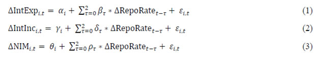 The estimates of banks’ expense and income betas are the sum of the coefficients of the contemporaneous and lagged estimates of ΔRepoRate in equation (1) to (3). Apart from all SCBs, the empirical analysis is also undertaken separately for public sector banks, private sector banks and foreign banks to assess if there are any differences across bank groups. In view of the sharp changes in interest rates in the first quarter of 2017 (in the aftermath of demonetisation), the regressions (1 to 3) were also estimated for the pre-demonetisation period (Q2:2010 to Q3:2016) for robustness. Furthermore, following Drechsler et al. (2017), a two-stage regression (equations 4 and 5, controlling for bank and time fixed effects) was also attempted to see if an individual bank’s interest income matches its interest expense. Results The estimates indicate that, for all SCBs, the coefficient of interest expense ratio (equation 1) on the policy interest rate was significantly different from zero and well below one, suggesting incomplete monetary transmission. The sensitivity is higher for public and private sector banks, but not significant for foreign banks (Table 1). Similarly, for all SCBs, the income betas estimated using equation 2 were significant but again much below unity (Table 2). As in the case of expense betas, the policy rate sensitivity to interest incomes was higher for public and private sector banks, and not significant for foreign banks. The coefficients of around 0.5 on the repo rate changes for both interest expenses and interest income in Tables 1 and 2 suggest that the policy rate changes do not impact banks’ NIMs. This is confirmed by direct estimates of NIMs in equation 3, with the coefficients being statistically insignificant (Table 3). The regression results for all SCBs for the pre-demonetisation sample (Q2:2010 to Q3:2016) were broadly similar to the full sample results (Table 4). The two-stage regression results indicate that the coefficient of the predicted interest expenses ratio (equation 5) was not statistically different from unity (Table 5). Further, the impact of changes in the policy rate turned out to be insignificant. This is found to be similar for all bank groups. These results suggest that, on average, Indian banks were able to protect the margins by transmitting changes in interest expenses to interest incomes.
Annex III.1 An Explanatory Note on Box Plot A box-whisker plot (also called as box plot) is a non-parametric approach for graphically representing the frequency distribution of a variable through their quartiles in form of a box. The middle line in the box represents the median and the upper and lower hinges of the box represent the 3rd and 1st quartiles (or 75th and 25th percentile) respectively. The length of the box represents the inter-quartile range which is a measure of dispersion. The spacing between the upper hinge and median, and median and lower hinge of the box indicates the degree of skewness in the data. The values which are outside 1.5 times the length of the box on either side are considered as outside value (or outliers) and represented as dots in the plot. The box-whisker plot also has lines extending vertically from the boxes called whiskers indicating variability outside the upper and lower quartiles. The upper and lower adjacent values represent the maximum and minimum of the series excluding outliers. Box-whisker plot can be represented as
Annex IV.1 IOSCO Principles for Benchmark The Board of the International Organization of Securities Commission (IOSCO) released a report titled “Principles for Financial Benchmarks” in July 2013 with a view to addressing the concerns over the fragility of benchmarks that had the potential to harm both investors and the real economy. These principles are intended to promote the reliability of benchmark determinations, and address benchmark governance, quality and accountability mechanisms as detailed below. Governance While constructing a good benchmark, it needs to be ensured that appropriate governance arrangements are put in place in order protect the integrity of the benchmark determination process and to address conflicts of interest. Governance, among the others, should emphasise that: (1) The Administrator should hold primary responsibility for all aspects of the benchmark determination process such as the development and determination of a benchmark and establishing credible and transparent governance, oversight and accountability procedures. This principle makes clear that regardless of the particular structure for benchmark determination and administration, there should be an overall entity which is responsible for the integrity of the benchmark. (2) The Administrator should adopt clearly defined written arrangements setting out the roles and obligations of the parties involved in the benchmark determination and the monitoring of any third party’s compliance with those arrangements. (3) To protect the integrity and independence of benchmark determination, Administrators should document, implement and enforce policies and procedures for the identification, disclosure, management, mitigation or avoidance of conflicts of interest. Administrators should disclose any material conflicts of interest to their users and relevant regulatory authority, if any. (4) An Administrator should implement an appropriate control framework for the process of determining and distributing the benchmark. The control framework should be appropriately tailored to the materiality of the potential or existing conflicts of interest identified, the extent of the use of discretion in the benchmark setting process and to the nature of benchmark inputs and outputs. The control framework should be documented and available to relevant regulatory authorities, if any. A summary of its main features should be published or made available to stakeholders. (5) Administrators should establish an oversight function to review and provide challenge on all aspects of the benchmark determination process. This should include consideration of the features and intended, expected or known usage of the benchmark and the materiality of existing or potential conflicts of interest identified. The oversight function and its composition should be appropriate to provide effective scrutiny of the Administrator. Quality of the Benchmark (6) The design of a benchmark should take into account generic design factors that are intended to result in a reliable representation of the economic realities of the interest that the benchmark seeks to measure and to eliminate factors that might result in a distortion of the price, rate, index or value of that benchmark. (7) The data used to construct a benchmark should be based on prices, rates, indices or values that have been formed by the competitive forces of supply and demand (i.e., in an active market) and be anchored by observable transactions entered into at arm’s length between buyers and sellers in the market for the interest the benchmark measures. Provided that an active market exists, conditions in the market on any given day might require the Administrator to rely on different forms of data tied to observable market data as an adjunct or supplement to transactions. Provided that an active market exists, Principle 7 does not preclude benchmark Administrators from using executable bids or offers as a means to construct benchmarks where anchored in an observable market consisting of bona fide, arm’s length transactions. For example, this approach might be appropriate in a market where overall transaction volume is high over sustained periods, though on any given day there might be more firm bids and offers than posted transactions taking place. The Principle also does not preclude the use of non-transactional data for indices that are not designed to represent transactions and where the nature of the index is such that non-transactional data is used to reflect what the index is designed to measure. (8) The establishment of clear guidelines regarding the hierarchy of data inputs and the exercise of expert judgment used for the determination of benchmarks which intended to make transparent to users the manner in which data and expert judgment may be used for the construction of a benchmark. (9) The publication with each benchmark determination, to the extent reasonable without delaying the Administrator’s publication deadline, of a concise explanation sufficient to facilitate a subscriber’s or market authority’s ability to understand how the benchmark determination was developed, as well as a concise explanation of the extent to which and the basis upon which judgment, if any, was used by the Administrator in establishing a benchmark determination. (10) The periodic review by the Administrator of the conditions in the underlying interest that the benchmark measures to determine whether the interest has undergone structural changes that might require changes to the design of the methodology (e.g., the interest has diminished to the extent that it can no longer function as the basis for a credible benchmark). Quality of the Methodology These principles are intended to promote the quality and integrity of methodology in public domain so that stakeholders may understand and make their own judgments concerning the overall credibility of a benchmark. The methodology should also keep the scope for informing stakeholders about any material changes in the underlying methodology, which might impact their positions, financial instruments or contracts. Administrators should have credible policies in case a benchmark ceases to exist or stakeholders need to transition to another benchmark. Specifically, these principles are: (11) The documentation and publication of the methodology used to make benchmark determination, with sufficient detail to allow stakeholders to understand how the benchmark is derived and to assess its representativeness, its relevance to particular stakeholders, and its appropriateness as a reference for financial instruments. (12) The publication of the rationale of any proposed material change in its Methodology, and procedures for making such changes. (13) Clearly written policies and procedures that address the need for possible cessation of a benchmark, due to market structure change, product definition changes, or any other condition, which makes the benchmark no longer representative of its intended function. These policies and procedures should be proportionate to the estimated breadth and depth of contracts and financial instruments that reference a benchmark and the economic and financial stability impact that might result from the cessation of the benchmark. (14) The development of guidelines for submitters (“Submitter Code of Conduct”), which should be available to any relevant regulatory authorities and published or made available to stakeholders. This principle is only applicable to a benchmark based on submissions. (15) Appropriate internal controls over the Administrator’s data collection and transmission processes – when an Administrator collects data directly from a regulated market, exchange or other data aggregator, which address the process for selecting the source, collecting the data and protecting the integrity and confidentiality of the data. Accountability These principles establish complaints processes, documentation standards and audit reviews that are intended to provide evidence of compliance by the Administrator with its quality standards, as defined by these principles and its own policies. Among the others, these principles address: (16) The establishment and publication of a written complaints policy by which stakeholders may submit complaints concerning whether a specific benchmark determination is representative of the underlying interest it seeks to measure, application of the methodology to a specific benchmark determination and other Administrator decisions in relation to a benchmark determination. (17) An appointment of an independent internal or external auditor with appropriate experience and capability to periodically review and report on the Administrator’s adherence to its stated criteria and the requirements of the principles. The frequency of audits should be proportionate to the size and complexity of the Administrator’s operations. (18) The retention of written records by the Administrator for five years, subject to applicable national legal or regulatory requirements to safeguard necessary documents for audits. Additional requirements apply for benchmarks based on submissions. (19) Relevant documents, audit trails and other documents addressed by these principles shall be made readily available by the relevant parties to the relevant regulatory authorities in carrying out their regulatory or supervisory duties and handed over promptly upon request. Source: The Board of the International Organization of Securities Commissions, “Principles for Financial Benchmarks”, Final Report (July 2013)
Annex IV.2a | Possible Candidates for Benchmark: Pros and Cons | | Benchmark | Methodology | Pros | Cons | | CD rate | Poll based rates (Reuters). | • Co-moves with the policy repo rate.
• Some properties of LIBOR.
- Linked to marginal cost of funds of banks.
- Also reflects banks’ credit risk to some extent.
- Term market exists, although not liquid.
• Least sensitive to global spillovers directly (FPIs not allowed).
• One of the least volatile money market rates in 2017. | • Volumes and rates - sensitive to credit cycle, liquidity conditions and seasonality.
• Based on polls and hence not in line with IOSCO Principles.
• Low volumes: Susceptible to manipulation. | | FBIL – CD rates | Transaction based. | • Transparent.
• Clear money market yield curve up to nine months maturity.
• Some properties of LIBOR, linked to cost of funds of banks.
• Also reflects banks’ credit risk to some extent.
• Least sensitive to global spillovers directly. | • Occasional mix of credit risk and risk free segments.
• All the cons relating to CDs mentioned above are applicable to FBIL-CD rates. | | T-Bill rates | Poll based rates (Reuters) as well as actual trades on NSE’s Wholesale Debt Market (WDM) and CCIL’s NDS OM system. | • Near risk free rate.
• Co-moves with the policy repo rate.
• Term market exists. | • May constrain future debt management operations.
• Volumes affected by fiscal and cash/debt management policies.
• Does not represent banks’ marginal cost of funds.
• Low depth exposes the market to the risk of manipulation.
• Globally not favoured because of sensitivity to sovereign risks (after the sovereign debt crisis) | | FBIL – TBs | Transaction based; (secondary market, NDS- OM) | • Transparent.
• Clear money market yield curve up to 1 year maturity. | • All the cons relating to TBs mentioned above are applicable here. | | Overnight Weighted Average Call Money Rate | Transaction based volume weighted average rate (CCIL). | • Reliable and transparent.
• Closely aligned to the policy repo rate. | • May constrain future changes in the operating framework of monetary policy.
• Volumes have declined in the recent period.
• No term structure.
• Volumes drop significantly on non-reporting Fridays (possibly shifting to 3-day tenor) and representative rates may not emerge on such days.
• Distorted by reported transactions1. | | Overnight CBLO Rate | • Robust, reliable and transparent.
• Closely aligned to the policy repo rate.
• Almost risk free rate.
• Largest overnight segment.
• Wider participation base. | • No term structure.
• Rate and volume drop on every reporting Friday.
• Susceptible to pressure on rates from mutual funds, which are major players. | | Market Repo Rate | • Robust, reliable and transparent.
• Closely aligned to the policy repo rate.
• Almost risk free rate.
• Wider participation base. | • No term structure.
• Rate and volumes drop on non-reporting Fridays. | | MIBOR | Transaction based volume weighted average rate - using NDS-Call transactions during the first hour (CCIL). | • Transparent.
• Not influenced by reported deals2.
• Co-moves with the policy repo rate.
• Used in the OIS market. | • Susceptible to manipulation.
• Not representative. | | MIFOR | Poll based, contributed by select panel of market participants (Reuters). | • Used for pricing interest rate swap (IRS) transactions.
• Term market exists, but remains underdeveloped. | • Not robust, susceptible to manipulation.
• Not representative. | | Overnight Index Swap (OIS) | FBIL (based on MIBOR) | • Term structure up to 10 years. | • Low market depth.
• Price discovery is not easy to understand.
• Concentrated market.
• All the cons relating to MIBOR are also applicable to OIS rates. | | Repo Rate | Announced by the MPC
(Based on assessment of macroeconomic conditions, consistent with the inflation targeting framework; as per the provisions of the amended RBI Act 1934). | • Robust, reliable and transparent.
• Simple and easy to understand.
• Cannot be manipulated.
• Marginal cost of funds for banks exhibit high correlation with the repo rate. | • May constrain future changes in the operating framework of monetary policy.
• Banks’ cost of funds linked to the Repo rate only at the margin (0.25 per cent of NDTL).
• Lack of a term curve. | | G-sec Yields | FIMMDA | • Transparent.
• Continuous term structure up to 30 years. | • Liquidity – concentrated at specific tenors.
• May constrain future debt management operations.
• Volumes affected by fiscal and cash/debt management policies.
• G-sec market does not represent marginal cost of funds for banks.
• Market is sensitive to regulatory, prudential and accounting norms.
• Vulnerable to global spillovers. | | 14-day Term Repo | RBI | • Robust, transparent and reliable. | • May constrain future changes in the operating framework of monetary policy.
• Access to liquidity under the 14- day term repo rate at 0.75 per cent of NDTL of the banking system as a whole.
• Not suitable in surplus liquidity conditions. | | Note: The pros and cons presented in this table reflect the personal views of the Study Group. | ________________________________________
Annex IV.2b | Possible Candidates for Benchmark: A Summary Assessment | | Instruments | Robustness | Correlation with the Policy Repo Rate | Liquidity | Linked to Banks’ Cost of Funds
(At the margin) | Existence of a Term Structure | Reliability and Transparency | | High | Low to Moderate | High | Low to Moderate | | WACR | ✓ | ✓ | | | ✓ | ✓ | x | ✓ | | CBLO | ✓ | ✓ | | ✓ | | ✓ | x | ✓ | | Market Repo | ✓ | ✓ | | | ✓ | ✓ | x | ✓ | | T-bill Rates | x | ✓ | | | ✓ | x | ✓ | x | | CD Rates | x | ✓ | | | ✓ | ✓ | ✓ | x | | MIBOR | ✓ | ✓ | | - | - | ✓ | x | x | | MIFOR | x | | ✓ | - | - | x | ✓ | x | | OIS | x | ✓ | | | ✓ | x | ✓ | x | | G-sec | ✓ | ✓ | | ✓ | | x | ✓ | ✓ | | FBIL (CD and T-bill) | x | ✓ | | - | - | ✓ | ✓ | ✓ | | 14-day Term Repo | ✓ | ✓ | | - | - | ✓ | - | ✓ | | Repo Rate | ✓ | - | - | - | - | ✓ | x | ✓ |
Annex IV.3 FBIL Certificates of Deposit (FBIL-CD) FBIL CD Curve (CDCURVE) is computed on a daily basis as per the following methodology: CDCURVE Computation Methodology 1. For the purpose of computation of the Benchmark CD Rates, secondary market transactions pertaining to scheduled commercial bank issuers with the highest rating reported to FTRAC platform and settling on T+0 basis are considered. Most of the trades reported to the Platform on daily basis are T+0. 2. The relevant trades are extracted after the close of market hours (typically at 5.00 PM). 3. All deals having value of Rs.5 crores and above are considered in the dataset. The trades are classified based on their residual maturity from the settlement date. These trades are then put into various time buckets representing the benchmark tenors of 14 days, 1 month, 2 months, 3 months, 6 months, 9 months and 12 months. The trades in each of these buckets serve as a medium for computation of a benchmark rate to represent a particular benchmark tenor. The following table is used for bucketing the transactions. | Trades Captured in Tenor Buckets – Classification based on Residual Maturity | | Bucket | Residual Maturity (days) | Benchmark Tenor | | 1 | 1 to 16 | 14 Days | | 2 | 17 to 45 | 1 Month | | 3 | 46 to 71 | 2 Months | | 4 | 72 to 115 | 3 Months | | 5 | 116 to 200 | 6 Months | | 6 | 201 to 300 | 9 Months | | 7 | >300 | 12 Months | 4. Once the trades are put into their respective tenor buckets, the weighted average rate is computed with the Standard Deviation of the rates, provided there are at least 3 trades in the tenor bucket. 5. Outliers are removed using +/-3SD criteria for each bucket. After such removal of outliers, if a tenor fails to have minimum trades of 3, the relevant Rate for the tenor is computed using relevant information from Treasury bill curve Rate (TBCURVE Rate) of FBIL as explained in point no 8. 6. For the purpose of computation of the Final Benchmark CD Curve Rate for a particular Tenor, the methodology takes into consideration four parameters, namely, the Distance, Volume, Amount and Rate. a. Distance: To calculate the Distance steps i to v as given below are followed: i. Calculate the difference between the residual tenors of a given trade with its respective benchmark tenor. For example, in case of trades with a residual tenor of 15 days, this difference is computed as 15 minus 14 which equals -1. ii. Calculate the absolute value of this difference. Following our example, |- 1| is equal to 1. iii. Calculate the sum of these absolute differences, for all trades in the relevant maturity bucket. If we have trades with the differences of 12, 8, 6 and 1 day, then this is the sum of 12, 8, 6 and 1 which equals to 27. iv. Each tenor is then assigned a weight, based on its percentage share in the sum of these absolute differences in that relevant bucket. In our case, this is equal to 0.0370, i.e., 1 (calculated from Step ii) divided by 27 (calculated from Step iii). v. Distance is then calculated as the inverse of this percentage share. In our example, this equals to 27, i.e., 1 divided by 0.0370. Thus, the parameter of Distance vary depending upon the proximity of the residual tenor of a given trade to its benchmark tenor. Indeed, given the benchmark tenor of 14 Days, trades with a residual tenor of 15 days will have a greater weight (i.e., a weight of 27) vis-à-vis trades with a residual tenor of 2 days (i.e., a weight of 2.25), as it lies closer to our benchmark tenor. b. Volume: The volume is computed as the percentage share of the number of trades (frequency), for a given residual tenor, in the total number of all the trades within that respective maturity bucket. As an example, there has been only one trade with a residual maturity of 15 days, within the 14 Days maturity bucket which consists of a cumulative of 5 trades. Hence the weight assigned to this trade is 0.20 (i.e., 1 divided by 5). Thus, larger the number of trades at a given tenor, greater would be its influence on the benchmark rate. c. Amount: For a given maturity bucket, the third parameter used in computation is the Amount (in crores) of all the trades which have a residual maturity that fall within that maturity bucket. The greater the value of the trades, the larger would be its weight in the computation process. For example, in case of the 1st maturity bucket, the trades with a residual maturity of 8 days and an amount of Rs. 70 crores will play a larger role in influencing the 14-Days benchmark rate vis-à-vis trades with a residual maturity of 15 days and an amount of Rs. 5 crores. Having computed the parameters, Weighted Average Rate (WAR) for each benchmark Tenor of the Curve is given by 7. Using the traded data, the Rates (yields) for each Tenor for the day are computed provided the Tenor has at least 3 surviving trades after outlier removal process. 8. If the Benchmark CDCURVE Rate for a Tenor is not available for a day, the said Rate is computed using the day’s Benchmark TBCURVE Rate for the relevant Tenor if such Rate has been calculated using trades or trades and executable orders of the T-Bills pertaining to the said tenor with a BID-ASK spread of 10 bps as the case may be (explained in detail in TB Rate Methodology document of FBIL) plus the traded spread of previous day (Difference between CDCURVE Rate and TBCURVE Rate if both are traded). 9. If the previous day’s traded spread is not available, then average of last 7 available spreads (Difference between traded CDCURVE Rate and TBCURVE Rate computed or calculated or interpolated with spreads) would be taken and added to the TBCURVE Rate for the relevant tenor for the Day to give the CDCURVE rate for the Tenor. 10. If CDCURVE Rate for a Tenor is not available for the day (no CD minimum trades and no T-Bills minimum trades), the CDCURVE Rate would be computed by using the previous day’s CD Rate (traded, computed with spread and repeated as the case may be) and the average spread of two adjacent CDCURVE Rates or the nearby spread as the case may be. 11. In case no CDCURVE Rate for a Tenor is possible to estimate for the second day, the CDCURVE Rate for the previous day would be repeated (maximum up to 2 days). 12. The rate is be published at about 5.30 PM subject to the calculation of TB Curve. If the TB curve estimation is delayed because of market time extension, CD curve Rate publication time will also suitably change. Depth of CD market in terms of volumes and number of trades is presented in Annex Tables IV.3.1 and IV.3.2. Source: FBIL | Annex Table IV.3.1: FBIL-CD Market Depth | | (Volume in Rs. crore) | | Date | 14-Days | 1-Month | 2-Month | 3-Month | 6-Month | 9-Month | 12-Month | | 23-Aug-17 | 120 | | | | 375 | | | | 24-Aug-17 | 200 | 425 | | 350 | 600 | | | | 28-Aug-17 | 150 | | 350 | 125 | 175 | | | | 29-Aug-17 | | 325 | | | | | | | 30-Aug-17 | | | | | | | | | 31-Aug-17 | 325 | 450 | | 125 | | 250 | | | 1-Sep-17 | 385 | | | 875 | 450 | | | | 4-Sep-17 | 155 | | 125 | | | | | | 5-Sep-17 | 275 | | | | 950 | | | | 6-Sep-17 | | 300 | | 125 | | | | | 7-Sep-17 | 105 | 100 | | | | | | | 8-Sep-17 | | | | | 600 | | | | 11-Sep-17 | | | | 650 | | | | | 12-Sep-17 | 1160 | | | | 250 | | | | 13-Sep-17 | | | | | 150 | | | | 14-Sep-17 | 595 | | 175 | 395 | | | | | 15-Sep-17 | 630 | | | | | | | | 18-Sep-17 | 325 | | | | | | | | 19-Sep-17 | 1295 | | 545 | | | 475 | | | 20-Sep-17 | 225 | 1850 | | 600 | | | | | 21-Sep-17 | 865 | 225 | 400 | 1785 | 250 | 250 | | | 22-Sep-17 | 905 | 125 | 250 | 975 | 400 | 125 | | | 25-Sep-17 | 1535 | | 575 | 2350 | | 525 | | | 26-Sep-17 | 840 | | 450 | 800 | | | | | Source: FBIL. |
| Annex Table IV.3.2: FBIL-CD Market Depth | | (Number of Trades) | | Date | 14-Days | 1-Month | 2-Month | 3-Month | 6-Month | 9-Month | 12-Month | | 23-Aug-17 | 3 | | | | 5 | | | | 24-Aug-17 | 4 | 5 | | 5 | 12 | | | | 28-Aug-17 | 4 | | 5 | 5 | 3 | | | | 29-Aug-17 | | 4 | | | | | | | 30-Aug-17 | | | | | | | | | 31-Aug-17 | 5 | 4 | | 4 | | 5 | | | 1-Sep-17 | 4 | | | 12 | 11 | | | | 4-Sep-17 | 3 | | 3 | | | | | | 5-Sep-17 | 3 | | | | 8 | | | | 6-Sep-17 | | 5 | | 3 | | | | | 7-Sep-17 | 3 | 3 | | | | | | | 8-Sep-17 | | | | | 7 | | | | 11-Sep-17 | | | | 8 | | | | | 12-Sep-17 | 18 | | | | 3 | | | | 13-Sep-17 | | | | | 4 | | | | 14-Sep-17 | 8 | | 3 | 9 | | | | | 15-Sep-17 | 7 | | | | | | | | 18-Sep-17 | 6 | | | | | | | | 19-Sep-17 | 15 | | 4 | | | 6 | | | 20-Sep-17 | 4 | 16 | | 5 | | | | | 21-Sep-17 | 11 | 3 | 5 | 27 | 6 | 4 | | | 22-Sep-17 | 10 | 4 | 5 | 14 | 5 | 3 | | | 25-Sep-17 | 15 | | 9 | 21 | | 4 | | | 26-Sep-17 | 10 | | 6 | 8 | | | | | Source: FBIL. |
Annex IV.4 FBIL Treasury Bills (FBIL-T Bill) FBIL Treasury Bill Curve (TBCURVE) is computed on daily basis as per the following methodology: TBCURVE Computation Methodology 1. For the purpose of computation of the Benchmark TB Rates, secondary market transactions - dealt and reported to NDS-OM platform - settling on T+1 basis are considered. 2. The trades and orders as and when relevant are extracted after the close of market hours, typically after 5.00 PM. 3. All deals having value of Rs.5 crores and above are considered in the dataset. No Constituent deals are taken for computation of the rates. The trades are classified based on their residual maturity from the settlement date. These trades then put into various time buckets representing the benchmark tenors of 14 days, 1 month, 2 months, 3 months, 6 months, 9 months and 12 months. The trades in each of these buckets serve as a medium for computation of a benchmark rate to represent a particular benchmark tenor. The following table is used for bucketing the transactions. | Trades Captured in Tenor Buckets – Classification on the basis of Residual | | Bucket | Residual Maturity (days) | Benchmark Tenor | | 1 | 1 to 16 | 14 Days | | 2 | 17 to 45 | 1 Month | | 3 | 46 to 71 | 2 Months | | 4 | 72 to 115 | 3 Months | | 5 | 116 to 200 | 6 Months | | 6 | 201 to 300 | 9 Months | | 7 | >300 | 12 Months | 4. Once the trades are put into their respective tenor buckets, the weighted average rate are computed with the Standard Deviation of the Rates, provided there are at least 3 trades in the tenor bucket. If there are less than 3 trades in a particular tenor, the weighted average rate and the Standard Deviation of the Rates are computed after augmenting the tenor point data with the executable orders with a maximum Bid-Ask spread of 10 bps of the T-Bills in NDS-OM system pertaining to that tenor bucket. The lower of the order values (of Buy and Sell orders) which satisfy the above criteria of 10 bps spread are included in volume to be used. 5. Outliers are removed using +/-3SD criteria for each bucket. The Benchmark TBCURVE Rate is computed if there are minimum of 3 surviving data points. If the surviving data point is less than 3, the fall back mechanism is kick in. 6. For the purpose of computation of the Final Benchmark TB Curve Rate for a particular Tenor, the methodology takes into consideration four parameters, namely, the Distance, Volume, Amount and Rate. a. Distance: To calculate the Distance, steps i to v as given under are followed: i. Calculate the difference between the residual tenors of a given trade with its respective benchmark tenor. For example, in case of trades with a residual tenor of 15 days, this difference is computed as 15 minus 14 which equals -1. ii. Calculate the absolute value of this difference. Following our example, |- 1| is equal to 1. iii. Calculate the sum of these absolute differences, for all trades in the relevant maturity bucket. If we have trades with the differences of 12, 8, 6 and 1 day, then this is the sum of 12, 8, 6 and 1 which equals to 27. iv. Each tenor is then assigned a weight, based on its percentage share in the sum of these absolute differences in that relevant bucket. In our case, this is equal to 0.0370, i.e., 1 (calculated from Step ii) divided by 27 (calculated from Step iii). v. Distance is then calculated as the inverse of this percentage share. In our example, this equals to 27, i.e., 1 divided by 0.0370. Thus, the parameter of Distance may vary depending upon the proximity of the residual tenor of a given trade to its benchmark tenor. Indeed, given the benchmark tenor of 14 Days, trades with a residual tenor of 15 days will have a greater weight (i.e., a weight of 27) vis-à-vis trades with a residual tenor of 2 days (i.e., a weight of 2.25), as it lies closer to our benchmark tenor. b. Volume: The volume is computed as the percentage share of the number of trades (frequency), for a given residual tenor, in the total number of all the trades within that respective maturity bucket. As an example, there has been only one trade with a residual maturity of 15 days, within the 14 Days maturity bucket which consists of a cumulative of 5 trades. Hence the weight assigned to this trade is 0.20 (i.e., 1 divided by 5). Thus, larger the number of trades at a given tenor, greater would be its influence on the benchmark rate. c. Amount: For a given maturity bucket, the third parameter used in computation is the Amount (in Rs. crores) of all the trades which have a residual maturity that fall within that maturity bucket. The greater the value of the trades, the larger would be its weight in the computation process. For example, in case of the 1st maturity bucket, the trades with a residual maturity of 8 days and an amount of Rs. 70 crores will play a larger role in influencing the 14-Days benchmark rate vis-à-vis trades with a residual maturity of 15 days and an amount of Rs. 5 crores. Having computed the parameters, Weighted Average Rate (WAR) for each benchmark Tenor of the Curve is given by 7. Using the traded data with augmentation wherever necessary, the Rates (yields) for each Tenor for the day are computed. 8. If the Benchmark TBCURVE Rate for a Tenor is not available for a day, the said Rate is computed using the previous day’s Benchmark TBCURVE Rate for the relevant Tenor plus the average spread of two adjacent buckets for the day (Ratet –Ratet-1). When two adjacent spread points are not available, the computation uses the nearest available spread for the Tenor. This results in having T-Bills Rates for almost all tenors on all days. 9. In case all attempts fail to estimate a Benchmark TBCURVE Rate for a particular Tenor on the Curve using the process explained above, previous day’s Rate for the appropriate Tenor is repeated. 10. If Benchmark TBCURVE Rates for all Tenors are not available for a day, the Benchmark TBCURVE of the previous day is repeated (maximum upto 2 days). 11. The Rates are published at about 5.30 PM. If the market time is extended, the publication time also suitably changes. Depth of T-Bill market in terms of volumes and number of trades is presented in Annex Tables IV.4.1 and IV.4.2. Source: FBIL | Annex Table IV.4.1: FBIL T- Bill Market Depth | | (Volume in Rs. crore) | | Date | 14-Days | 1-Month | 2-Month | 3-Month | 6-Month | 9-Month | 12-Month | | 23-Aug-17 | 480 | 535 | | 575 | 1950 | 300 | 125 | | 24-Aug-17 | 260 | 110 | | 350 | 228 | 60 | 100 | | 28-Aug-17 | | 445 | 405 | 485 | 520 | 255 | 75 | | 29-Aug-17 | 760 | 25 | 360 | 1395 | 150 | 250 | | | 30-Aug-17 | | 110 | 280 | 5117 | 225 | | 375 | | 31-Aug-17 | | | 145 | 1062 | 475 | 279 | 410 | | 1-Sep-17 | | 845 | 200 | 145 | 455 | | 175 | | 4-Sep-17 | 80 | 960 | 445 | 745 | 475 | | 305 | | 5-Sep-17 | 220 | 755 | 935 | 935 | 1560 | | 190 | | 6-Sep-17 | | 595 | | 4655 | 6914 | 542 | 575 | | 7-Sep-17 | 1095 | | 230 | 1650 | 585 | | 80 | | 8-Sep-17 | 500 | | | 750 | 130 | | 185 | | 11-Sep-17 | 1425 | 315 | 40 | 1340 | 325 | | | | 12-Sep-17 | 955 | 563 | 530 | 155 | 520 | 535 | | | 13-Sep-17 | 1175 | 560 | | 4818 | 900 | 490 | 1082 | | 14-Sep-17 | 1175 | 589 | 105 | 430 | 760 | | 230 | | 15-Sep-17 | | 3275 | | 265 | 400 | | 30 | | 18-Sep-17 | 2482 | 1170 | | 270 | 85 | | 160 | | 19-Sep-17 | 2660 | 985 | | 285 | 795 | | 170 | | 20-Sep-17 | 350 | 145 | | 6635 | 1513 | 165 | | | 21-Sep-17 | 755 | 370 | 450 | 535 | 1930 | 350 | 195 | | 22-Sep-17 | 365 | 120 | 35 | 1702 | 210 | 495 | 75 | | 25-Sep-17 | 702 | | 155 | 331 | 1532 | 90 | 80 | | 26-Sep-17 | 1000 | 210 | 265 | 75 | 1355 | 55 | | | Source: FBIL |
| Annex Table IV.4.2: FBIL T-Bill Market Depth | | (Number of Trades) | | Date | 14-Days | 1-Month | 2-Month | 3-Month | 6-Month | 9-Month | 12-Month | | 23-Aug-17 | 8 | 10 | | 15 | 21 | 5 | 3 | | 24-Aug-17 | 4 | 3 | | 10 | 10 | 4 | 4 | | 28-Aug-17 | | 9 | 3 | 6 | 13 | 5 | 4 | | 29-Aug-17 | 12 | 3 | 6 | 17 | 3 | 3 | | | 30-Aug-17 | | 9 | 3 | 28 | 6 | | 11 | | 31-Aug-17 | | | 3 | 30 | 12 | 3 | 7 | | 1-Sep-17 | | 7 | 3 | 4 | 9 | | 4 | | 4-Sep-17 | 6 | 12 | 10 | 13 | 9 | | 12 | | 5-Sep-17 | 4 | 7 | 4 | 11 | 8 | | 3 | | 6-Sep-17 | | 7 | | 40 | 45 | 5 | 10 | | 7-Sep-17 | 8 | | 4 | 38 | 15 | | 7 | | 8-Sep-17 | 11 | | | 19 | 3 | | 4 | | 11-Sep-17 | 19 | 5 | 4 | 28 | 10 | | | | 12-Sep-17 | 12 | 6 | 4 | 3 | 4 | 6 | | | 13-Sep-17 | 19 | 4 | | 143 | 25 | 9 | 14 | | 14-Sep-17 | 11 | 8 | 4 | 5 | 11 | | 9 | | 15-Sep-17 | | 13 | | 8 | 11 | | 3 | | 18-Sep-17 | 24 | 10 | | 4 | 5 | | 4 | | 19-Sep-17 | 19 | 8 | | 4 | 11 | | 4 | | 20-Sep-17 | 11 | 4 | | 68 | 12 | 4 | | | 21-Sep-17 | 11 | 5 | 4 | 11 | 17 | 9 | 3 | | 22-Sep-17 | 4 | 4 | 3 | 11 | 9 | 12 | 3 | | 25-Sep-17 | 22 | | 3 | 9 | 11 | 6 | 3 | | 26-Sep-17 | 13 | 3 | 5 | 3 | 14 | 3 | | | Source: FBIL |
ABBREVIATIONS | AMFI | Association of Mutual Funds in India | | ARRC | Alternative Reference Rates Committee | | ASIC | Australian Securities and Investments Commission | | AUM | Assets Under Management | | BIS | Bank for International Settlements | | BPLR | Benchmark Prime Lending Rate | | bps | basis points | | CASA | Current and Savings Account | | CBLO | Collateralised Borrowing and Lending Obligation | | CCIL | Clearing Corporation of India Limited | | CDs | Certificates of Deposit | | CGM | Chief General Manager | | CIBIL | Credit Information Bureau (India) Limited | | CPs | Commercial Papers | | CRR | Cash Reserve Ratio | | DBR | Department of Banking Regulation | | DBS | Department of Banking Supervision | | DRI | Differential Rate of Interest | | ECB | European Central Bank | | ELSS | Equity Linked Savings Scheme | | EMEs | Emerging Market Economies | | EONIA | Euro OverNight Index Average | | EURIBOR | Euro Inter-bank Offered Rate | | FBs | Foreign Banks | | FBIL | Financial Benchmark India Private Limited | | FCA | Financial Conduct Authority | | FII | Foreign Institutional Investor | | FINSIA | Financial Services Institute of Australasia | | FIMMDA | Fixed Income Money Markets and Derivatives Association | | FMRD | Financial Markets Regulation Department | | FPI | Foreign Portfolio Investor | | FSB | Financial Stability Board | | FSU | Financial Stability Unit | | F-TRAC | FIMMDA Trade Reporting and Confirmation System | | GFMA | Global Financial Market Association | | GNPA | Gross Non-Performing Assets | | G-Secs | Government Securities | | G20 | Group of Twenty | | HNIs | High Networth Individuals | | IBOR | Inter-bank Offered Rate | | IOSCO | International Organization of Securities Commissions | | IMF | International Monetary Fund | | IRS | Interest Rate Swap | | INBMK | Indian Benchmark | | IND-AS | Indian Accounting Standard | | LAF | Liquidity Adjustment Facility | | LCR | Liquidity Coverage Ratio | | LIBOR | London Inter-bank Offered Rate | | MCLR | Marginal Cost of Funds Based Lending Rate | | MIBOR | Mumbai Inter-bank Outright Rate | | MIFOR | Mumbai Inter-bank Forward Offer Rate | | MPC | Monetary Policy Committee | | MPD | Monetary Policy Department | | MSF | Marginal Standing Facility | | MSMEs | Micro, Small and Medium Enterprises | | NDTL | Net Demand and Time Liabilities | | NDS-CALL | Negotiated Dealing System-Call | | NDS-OM | Negotiated Dealing System-Order Matching | | NIM | Net Interest Margin | | NPA | Non-performing Asset | | NSE | National Stock Exchange | | NSFR | Net Stable Funding Ratio | | OBFR | Overnight Bank Funding Rate | | OIS | Overnight Indexed Swap | | OTC | Over the Counter | | PLR | Prime Lending Rate | | PSBs | Public Sector Banks | | PvtSBs | Private Sector Banks | | RBI | Reserve Bank of India | | RFRs | Risk Free Benchmark Rates | | RHS | Right Hand Side | | RoA | Return on Assets | | RoNW | Return on Net Worth | | RRBs | Regional Rural Banks | | SBI | State Bank of India | | SCBs | Scheduled Commercial Banks | | SEBI | Securities and Exchange Board of India | | SFBs | Small Finance Banks | | SG | Study Group | | SLR | Statutory Liquidity Ratio | | SMEs | Small and Medium Enterprises | | SONIA | Sterling Overnight Inter-bank Average Rate | | T-Bill | Treasury Bill | | TB | Treasury Bill | | TIBOR | Tokyo Inter-bank Offered Rate | | TONAR | Tokyo Overnight Average Rate | | UK | United Kingdom | | US | United States | | USD | United States Dollar | | WACR | Weighted Average Call Money Rate | | WADTDR | Weighted Average Domestic Term Deposit Rate | | WAEIR | Weighted Average Effective Interest Rate | | WALR | Weighted Average Lending Rate | | WALR-F | Weighted Average Lending Rate on Fresh Rupee Loans | | WALR-O | Weighted Average Lending Rate on Outstanding Rupee Loans | | WAR | Weighted Average Rate | | WDM | Wholesale Debt Market | | Y-o-y | Year-on-Year | |