| I. Macroeconomic Outlook The slowdown in domestic economic activity that started in 2018-19 extended into the first half of 2019-20. Headline consumer price index (CPI) inflation is projected to remain below target over the rest of 2019-20 and the early months of 2020-21. Real gross domestic product (GDP) growth is expected to recover in H2:2019-20, facilitated by favourable base effects and transmission of past monetary policy actions. A slew of measures by the government impart an upside to growth prospects. Intensification of global uncertainty around US-China trade tensions, a hard Brexit and geo-political tensions are key downside risks to the baseline growth path. I.1 Key Developments since April 2019 MPR Since the release of the Monetary Policy Report (MPR) of April 2019, global economic activity has weakened further. Several downside risks flagged in the April MPR appear to be materialising: escalation of trade tensions; growing probability of a disorderly Brexit; volatility in crude oil prices; and a risk-on risk-off sentiment in financial markets on tumultuous geo-political and economic events. In their wake, global growth has lost the momentum it had gathered in Q1:2019. Central banks across advanced economies (AEs) and emerging market economies (EMEs) are easing monetary policy in counter-cyclical defence. Global trade has sunk into contraction, with knock-on effects impacting investment and industrial production, especially manufacturing. Reflecting this, commodity prices slumped, with crude oil prices tumbling in August and gold prices surging on safe haven demand. Foreign exchange markets turned volatile, following the depreciation of the Chinese renminbi in early August. Crude oil prices were bolstered temporarily in mid-September by the attack on Saudi Arabian oil facilities and disruption to global oil supplies. Domestically, the slowdown in economic activity that started in 2018-19 extended into the first half of 2019-20. Real GDP growth fell to a 25-quarter low in Q1:2019-20 on weak private consumption and investment and high frequency indicators for Q2 point to a slowdown in the various constituents of aggregate demand deepening. Some green shoots are emerging though in agriculture and allied activities. The initial delay and deficiency in the south-west monsoon has been mitigated by the resurgence of rains during July-September. Comfortable reservoir levels augur well for rabi sowing and foodgrains stocks above the buffer norms provide a cushion against potential inflationary pressures. Meanwhile, headline CPI inflation remains below target. While food inflation has edged up since March 2019, inflation excluding food and fuel has undergone a broad-based moderation. Monetary Policy Committee: April-August 2019 During April-August 2019, the Monetary Policy Committee (MPC) met thrice in accordance with the bi-monthly schedule. In the April meeting, the MPC cut the repo rate by 25 basis points (bps) to 6.0 per cent (with a majority vote of 4-2) to strengthen domestic growth impulses by spurring private investment, while maintaining a neutral stance (with a majority vote of 5-1). With signs of weakening of growth impulses even further widening the negative output gap, and with headline inflation projected to remain below the target over the next 12 months, the MPC voted unanimously to reduce the repo rate by another 25 bps in its June 2019 meeting and changed the stance of monetary policy from neutral to accommodative. In its August meeting, the MPC reduced the policy repo rate by a further 35 bps to 5.40 per cent on signs of accentuation of the slowdown in domestic activity amidst deteriorating global growth and escalating trade tensions posing downside risks to the outlook. With the inflation outlook projected to be benign and within the target over the forecast horizon, all members of the MPC voted unanimously to reduce the policy rate (4 members for a reduction of 35 bps and two for 25 bps) and to maintain an accommodative stance. The MPC was of the view that the standard 25 bps cut might prove to be inadequate in view of evolving global and domestic macroeconomic developments, while a 50 bps reduction might be excessive, especially taking into account the actions already undertaken. Overall, the MPC reduced the policy repo rate by a cumulative 85 bps during April-August, in addition to the reduction of 25 bps in February. The MPC’s voting pattern reflects the diversity in individual members’ assessments, expectations and policy preferences, a feature that is reflected in voting patterns of the MPC in other central banks (Table I.1). Macroeconomic Outlook Chapters II and III analyse the macroeconomic developments during April-September 2019 and explain deviations of inflation and growth outcomes vis-à-vis staff’s projections. Turning to the outlook, the evolution of key macroeconomic and financial variables over the past six months warrants revisions in the baseline assumptions (Table I.2). | Table 1.1: Monetary Policy Committees and Voting Pattern | | Country | Policy Meetings: April 2019 - September 2019 | | Total Meetings | Meetings with Full Consensus | Meetings with Dissents | | Brazil | 4 | 4 | 0 | | Chile | 4 | 3 | 1 | | Czech Republic | 4 | 2 | 2 | | Hungary | 5 | 5 | 0 | | Israel | 4 | 1 | 3 | | Japan | 4 | 0 | 4 | | South Africa | 3 | 2 | 1 | | Sweden | 3 | 3 | 0 | | Thailand | 4 | 3 | 1 | | UK | 4 | 4 | 0 | | US | 4 | 1 | 3 | | Sources: Central bank websites. |
| Table I.2: Baseline Assumptions for Near-Term Projections | | Indicator | MPR (April 2019) | Current MPR (October 2019) | | Crude oil (Indian basket) | US$ 67.0 per barrel during 2019-20 | US$ 62.6 per barrel | | Exchange rate | ₹69/US$ | ₹71.3/US$ | | Monsoon | Normal for 2019 | 10 per cent above long period average | | Global growth | 3.5 per cent in 2019
3.6 per cent in 2020 | 3.2 per cent in 2019
3.5 per cent in 2020 | | Fiscal deficit (per cent of GDP) | To remain within BE 2019-20
Centre: 3.4
Combined: 5.9 | To remain within BE 2019-20
Centre: 3.3
Combined: 5.9 | | Domestic macroeconomic/ structural policies during the forecast period | No major change | No major change | Notes: 1. The Indian basket of crude oil represents a derived numeraire comprising sour grade (Oman and Dubai average) and sweet grade (Brent) crude oil.
2. The exchange rate path assumed here is for generating staff’s baseline growth and inflation projections and does not indicate any ‘view’ on the level of the exchange rate. The Reserve Bank is guided by the objective of containing excess volatility in the foreign exchange market and not by any specific level of and/or band around the exchange rate.
3. Global growth projections are from the World Economic Outlook (January and July 2019 Updates), International Monetary Fund (IMF).
4. BE: Budget estimates.
5. Combined fiscal deficit refers to that of the Centre and States taken together.
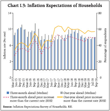
Sources: RBI staff estimates; Budget documents; and IMF. | First, international crude oil prices declined between mid-May and mid-September reflecting weakness in global demand amidst excess supply conditions and large stockpiles, despite geo-political tensions and production cuts by the Organisation of the Petroleum Exporting Countries (OPEC) (Chart I.1). Crude oil prices hardened temporarily in the second half of September following disruptions to production in Saudi Arabia. Given the current demand-supply assessment, the baseline scenario assumes crude oil prices at an average of US$ 62.6 per barrel. 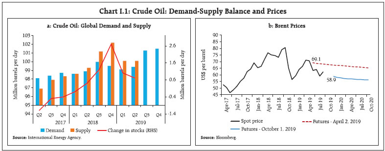 Second, the nominal exchange rate (Indian rupee, INR vis-à-vis the US dollar) has depreciated from its April level, especially during August, impacted by a drop in the Chinese renminbi below the psychological level of 7 yuan per US$ in the wake of an escalation in US-China trade actions. A generalised flight to safety towards the US dollar assets and portfolio capital outflows also amplified pressures on the rupee. The rupee came under renewed pressure in mid-September following the spike in crude oil prices but recovered in subsequent days following the announcement of various measures by the government to boost investment and growth and to stabilise the flow of funds into the capital market. Third, the weakening of global economic activity and trade is confirmed by the global manufacturing purchasing managers’ index (PMI) remaining in contraction zone in September 2019 at 49.7, the World Trade Organisation's Goods Trade Barometer indicating weakness in merchandise trade persisting in Q3:2019 and downgrades to global growth projections by various agencies. Against this backdrop, global growth for 2019 and 2020 is now expected to be below the April baseline (Table I.2 and Chart I.2). I.2 The Outlook for Inflation Headline CPI inflation has remained below target so far in 2019-20. Importantly, inflation excluding food and fuel has softened across major goods and services, reflecting the slowdown in domestic demand. Looking ahead, inflation expectations feed into future inflation through price and wage contracts. One-year ahead inflation expectations of urban households increased by 20 bps over the previous round in the September round of the survey conducted by the Reserve Bank; three-month ahead inflation expectations moved up by 40 bps during this period (Chart I.3).1 According to the Reserve Bank’s consumer confidence survey for September, inflation expectations moderated from the previous round. 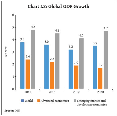
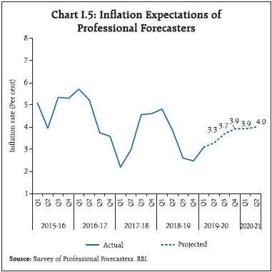
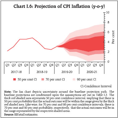
 Manufacturing firms polled in the July-September 2019 round of the Reserve Bank’s Industrial Outlook Survey (IOS) expected an increase in the cost of raw materials and muted selling prices in Q3:2019-20 (Chart I.4).2 According to the purchasing managers’ survey for manufacturing firms, input prices eased in September due to weak demand for raw materials and semi-finished items; output prices registered a marginal increase. Services sector firms reported lower input prices and higher output prices in August. Professional forecasters surveyed by the Reserve Bank in September 2019 expected CPI inflation to increase from 3.2 per cent in August 2019 to 3.9 per cent in Q4:2019-20 and to 4.0 per cent in Q2:2020-21 (Chart I.5).3 Taking into account the initial conditions, the signals from forward-looking surveys and estimates from time-series and structural models, CPI inflation is projected at 3.4 per cent in Q2:2019-20, 3.5 per cent in Q3, and 3.7 per cent in Q4, with risks evenly balanced (Chart I.6). The 50 per cent and the 70 per cent confidence intervals for headline inflation in Q4:2019-20 are 2.7-4.7 per cent and 2.2-5.3 per cent, respectively. For 2020-21, assuming normal monsoon and no major exogenous or policy shocks, structural model estimates indicate that inflation will move in a range of 3.5-4.0 per cent. The 50 per cent and the 70 per cent confidence intervals for Q4:2020-21 are 2.5-5.4 per cent and 1.8-6.2 per cent, respectively. 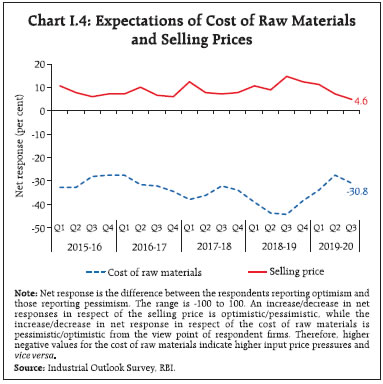
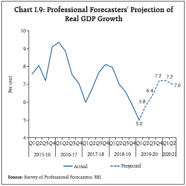
 There are both upside and downside risks to the baseline inflation forecasts. The upside risks include: volatility in international and domestic financial markets from trade tensions, Brexit and monetary policy stances of the major AEs; supply disruptions in the global crude oil market due to geo-political tensions; and, sudden spikes in the prices of perishable food items. Downside risks could emanate from more than assumed softening in crude oil and other commodity prices due to sluggish global demand, and weaker inflation excluding food and fuel domestically due to depressed domestic demand conditions. I.3 The Outlook for Growth As indicated earlier, domestic economic activity turned out to be weaker in H1:2019-20 vis-à-vis projections in the April 2019 MPR in an environment of global headwinds. The expected pick-up in both private consumption and investment failed to materialise, and exports lost momentum under the weight of the slump in world trade. Although the south-west monsoon turned out to be above long period average, its uneven progress – both temporal and spatial – could impinge upon the prospects for agriculture. Turning to the outlook, consumer confidence for the year ahead moved lower in the May, July and September rounds of the Reserve Bank’s survey, due to ebbing of sentiments on the general economic situation and the employment scenario (Chart I.7).4 Sentiment in the manufacturing sector polled in the July-September 2019 round of the Reserve Bank’s IOS dipped for the quarter ahead, reflecting moderation in expected production, order inflows, capacity utilisation, employment conditions and exports (Chart I.8). Surveys by other agencies of future business expectations indicate a mixed picture (Table I.3). Firms in the manufacturing and services sectors polled in the Nikkei’s purchasing managers’ surveys were optimistic about one-year ahead output prospects. In the September 2019 round of the Reserve Bank’s survey, professional forecasters expected real GDP growth to recover from 5.0 per cent in Q1:2019-20 to 7.2 per cent in Q4:2019-20 and then moderate to 7.0 per cent in Q2:2020-21 (Chart I.9). Taking into account the baseline assumptions, survey indicators, the reductions in the policy repo rate since February 2019, the base effects and model forecasts, real GDP growth is projected at 6.1 per cent in 2019-20 – 5.3 per cent in Q2, 6.6 per cent in Q3, 7.2 per cent in Q4 – with risks evenly balanced (Table I.4). For 2020-21, the structural model estimates indicate real GDP growth at 7.0 per cent – quarterly growth rates in the range of 6.5-7.4 per cent – assuming a normal monsoon, and no major exogenous or policy shocks. | Table I.3: Business Expectations Surveys | | Item | NCAER Business Confidence Index (July 2019) | FICCI Overall Business Confidence Index (June 2019) | Dun and Bradstreet Composite Business Optimism Index (July 2019) | CII Business Confidence Index (September 2019) | | Current level of the index | 121.8 | 59.6 | 70.0 | 52.5 | | Index as per previous survey | 115.4 | 60.3 | 78.4 | 59.6 | | % change, q-o-q | 5.5 | -1.2 | -10.7 | -11.9 | | % change, y-o-y | 6.5 | -16.1 | -13.2 | -19.1 | Notes: 1. NCAER: National Council of Applied Economic Research.
2. FICCI: Federation of Indian Chambers of Commerce & Industry.
3. CII: Confederation of Indian Industry. |
| Table I.4: Projections - Reserve Bank and Professional Forecasters | | (Per cent) | | | 2019-20 | 2020-21 | | Reserve Bank’s Baseline Projection | | | | Inflation, Q4 (y-o-y) | 3.7 | 4.0 | | Real GDP Growth | 6.1 | 7.0 | | Median Projections of Professional Forecasters | | | | Inflation, Q4 (y-o-y) | 3.9 | 4.0# | | Real GDP growth | 6.2 | 7.0 | | Gross domestic saving (per cent of GNDI) | 30.1 | 30.5 | | Gross capital formation (per cent of GDP) | 31.0 | 31.0 | | Credit growth of scheduled commercial banks | 12.0 | 12.9 | | Combined gross fiscal deficit (per cent of GDP) | 6.1 | 6.0 | | Central government gross fiscal deficit (per cent of GDP) | 3.3 | 3.3 | | Repo rate (end-period) | 5.0 | - | | Yield on 91-days treasury bills (end-period) | 5.2 | 5.4 | | Yield on 10-year central government securities (end-period) | 6.3 | 6.5 | | Overall balance of payments (US$ billion) | 15.1 | 10.0 | | Merchandise exports growth | 1.5 | 6.3 | | Merchandise imports growth | 0.5 | 7.1 | | Current account balance (per cent of GDP) | -1.9 | -2.0 | Note: GNDI: Gross National Disposable Income.
#: Q2:2020-21.
Source: RBI staff estimates; and Survey of Professional Forecasters (September 2019). |
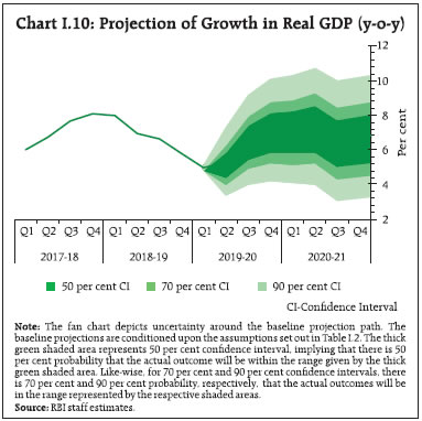 There are upside as well as downside risks to the baseline growth scenario (Chart I.10). The measures announced by the government in August-September to boost growth and investment – policy reforms on foreign direct investment (FDI), upfront release of funds for recapitalisation of public sector banks (PSBs), merger of PSBs, incentives for exports and real estate, reduction in the corporate income tax rate – along with a faster resolution of stressed assets, and a faster pace of transmission of past repo rate cuts by banks to their lending rates impart an upward bias to the baseline growth projection path. However, further escalation of trade tensions, a hard or no-deal Brexit and increased volatility in global financial markets pose downside risks to the baseline growth path. I.4 Balance of Risks The baseline projections of inflation and growth in the preceding sections are conditional on the assumptions relating to the key variables set out in Table I.2. Uncertainties surrounding these assumptions could lead to upward and downward deviations from baseline projections. This section assesses the balance of risks to the baseline projections in plausible alternative scenarios. (i) Global Growth Uncertainties The baseline scenario assumes a slowdown in external demand in 2019 and 2020. Yield curve inversion in major AEs has raised concerns about the growth outlook (Box I.1). Global growth could turn out to be weaker if there is further escalation of trade tensions, a hard/no-deal Brexit, a greater-than-envisaged slowdown in some major economies like China, or a combination of these factors. In such a scenario, if global growth slips down by 50 bps vis-à-vis the baseline, domestic growth and inflation could be lower by around 20 bps and 10 bps, respectively, from their baseline trajectories (Charts I.11a and I.12a). Conversely, an expeditious and orderly resolution of trade tensions, and/or a smooth Brexit could boost confidence and provide support to global trade and demand. Should global growth surprise by 50 bps on the upside, domestic growth and inflation could edge higher by around 20 bps and 10 bps, respectively. 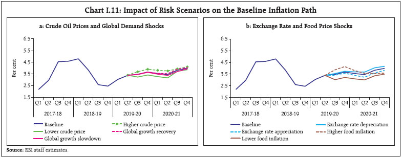
Box I.1: Does Yield Spread Predict Output Growth? The spread between yields on the US 10-year and 3-month treasury securities – a closely watched metric for term spread – has inverted for the first time since 2007 and turned negative at 13 basis points (bps) in June 2019. The spread has remained in negative territory for the third consecutive month in August at 35 bps (from 83 bps a year ago). Since the 1950s, US recessions have been preceded by sizeable inversions in the yield curve. The only occasion when the 3-month Treasury security yield exceeded the 10-year Treasury yield without the occurrence of a subsequent recession was in September 1966. Barring this, yield curve inversion has coincided with a recession in the following 18-24 months (Chart I.1.1a). Inversion/narrowing of yield spreads has occurred in other AEs. Yields have flattened in Germany, the UK, Japan, Singapore and Australia, mirroring a slowdown in the global economy. In the case of Germany, the spread of the 10-year bond yield over the 3-month bond yield turned negative falling to 24 bps in August 2019 as compared with 61 bps a year ago. Germany experienced recessions beginning in 1966, 1973, 1980, 1991, 2001 and 2008. All recessions, except the 1966 recession, were preceded by a sharp decline in long-term Treasury security yields relative to short-term yields. The only inversion that was not followed by a recession was in 1970 (Chart I.1.1b). 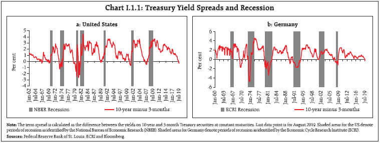 According to the expectations hypothesis of the term structure, long-term interest rates equal the sum of current and expected future short-term interest rates plus a term premium. The term premium explains why the yield curve usually slopes upwards, i.e., yields on long-term securities usually exceed those on short-term securities. The yield curve flattens or inverts/slopes downward when the public expects short-term interest rates to fall. In such a scenario, investors bid up the prices of longer-term securities causing a fall in long-term yields relative to yield on short-term securities. There is no unanimity, however, on the theoretical relationship between the term spread and economic activity. To a large extent, the usefulness of the spread for forecasting economic activity remains a “stylised fact in search of a theory” (Benati and Goodhart, 2008). Moreover, the predictive power of the term spread for output growth depends on monetary policy objectives and the reaction function used. In the case of monetary policy tightening for example, short-term rates are likely to rise more than long-term rates and cause the yield curve to flatten or possibly invert (Feroli, 2004). It is also argued that the term spread forecasts output growth better, the more responsive the monetary authority is to deviations of output from potential. The spread forecasts less accurately if monetary policy focusses exclusively on controlling inflation. The consumption smoothing model derives a relationship between the slope of the yield curve and future economic activity by assuming that individuals prefer stable consumption rather than high consumption during periods of rising income and low consumption when income is falling (Harvey, 1988). If they expect a recession in the future, consumers sell short-term financial instruments and purchase bonds at a discount to generate income, resulting in a flattening or inversion of the yield curve. | Table I.1.1: Correlation between GDP Growth and Yield Spreads | | | Lagged Yield Spread | | Future Yield Spread | | Country | t-6 | t-5 | t-4 | t-3 | t-2 | t-1 | t | t+1 | t+2 | t+3 | t+4 | t+5 | t+6 | | US | 0.136 | 0.192 | 0.218 | 0.213 | 0.229 | 0.154 | 0.041 | -0.073 | -0.166 | -0.204 | -0.231 | -0.341 | -0.360 | | | (0.042) | (0.004) | (0.001) | (0.001) | (0.001) | (0.021) | (0.545) | (0.278) | (0.013) | (0.002) | (0.001) | (0.000) | (0.000) | | Germany | 0.268 | 0.272 | 0.307 | 0.291 | 0.322 | 0.119 | -0.026 | -0.207 | -0.372 | -0.385 | -0.400 | -0.418 | -0.311 | | | (0.037) | (0.034) | (0.016) | (0.023) | (0.011) | (0.361) | (0.843) | (0.110) | (0.003) | (0.002) | (0.001) | (0.001) | (0.015) | Notes: 1. Yield spread between 10-year and 3-month Treasury securities has been measured as the quarterly average of monthly observations.
2. Data for the US and Germany pertain to the period Q2:1962–Q2:2019 and Q4:2002–Q2:2019, respectively.
3. Figures in the parentheses represent p-values.
Sources: Bloomberg; and RBI staff estimates. | The empirical literature suggests that the yield spread predicts output growth at a four-to-six-quarter horizon with considerable variation across countries and over time. However, the ability of the term spread to forecast output growth has declined since the mid-1980s (Wheelock and Wohar, 2009). On the other hand, probit models show that the yield spread outperforms in relation to other macroeconomic and financial variables while predicting the probability of recession (Estrella and Hardouvelis, 1991; Estrella and Mishkin, 1998). The contemporaneous correlation between the yield spread and real GDP growth was found to be statistically insignificant for both the US and Germany (Table I.1.1). However, correlations between GDP growth and the yield spread lagged by one to six quarters were found to be positive and statistically significant for both the countries, except for the period t-1 for Germany, where it was found to be insignificant. These correlations suggest that the steeper is the yield curve – higher the yield on 10-year Treasury securities relative to that on 3-month Treasury securities – the higher is the future rate of GDP growth. Similarly, correlations between GDP growth and future yield spreads up to six quarters have been found to be negative and statistically significant for both countries, except for period t+1 where it is insignificant for both countries. Negative correlations between GDP growth and the lead terms of the yield spread suggest that higher the GDP growth in period t, less steep would be the yield curve in subsequent quarters (Sahoo and Gupta, 2019). To sum up, the yield spread has been useful in predicting output growth and recessions at least up to one year in advance, particularly in major AEs, although its signalling value has somewhat blurred in the present environment of unconventional monetary policies. The current phase of negative yield spreads warrants that policymakers remain vigilant. References: Benati, L. and C. Goodhart (2008), “Investigating Time-Variation in the Marginal Predictive Power of the Yield Spread”, Journal of Economic Dynamics and Control, 32(4), pp. 1236-72. Estrella, A. and G. A. Hardouvelis (1991), “The Term Structure as a Predictor of Real Economic Activity”, Journal of Finance, 46(2), pp. 555-76. Estrella, A. and F. S. Mishkin (1998), “Predicting U.S. Recessions: Financial Variables as Leading Indicators”, Review of Economics and Statistics, 80(1), pp. 45-61. Feroli, M. (2004), “Monetary Policy and the Information Content of the Yield Spread”, Topics in Macroeconomics, 4(1), Article 13. Harvey, C. R. (1988), “The Real Term Structure and Consumption Growth”, Journal of Financial Economics, 22(2), pp. 305-33. Sahoo, S. and B. Gupta (2019), ';Does Yield Spread Predict Output Growth?';, Reserve Bank of India (Mimeo). Wheelock, D. C. and M. E. Wohar (2009), “Can the Term Spread Predict Output Growth and Recessions? A Survey of the Literature”, Federal Reserve Bank of St. Louis Review, September/October. | (ii) International Crude Oil Prices The Indian basket of crude oil prices has exhibited high volatility in the first half of 2019-20 and the outlook remains uncertain. Upside risks to the baseline assumption can emanate from geo-political tensions. Assuming crude oil prices increase to US$ 73 per barrel, inflation could be higher by around 30 bps and growth weaker by around 20 bps from the baseline. Conversely, crude oil prices could soften further if global demand turns out to be weaker than expected. Should the price of the Indian basket of crude fall to US$ 53, inflation could ease by around 30 bps and growth could be higher by around 20 bps (Charts I.11a and I.12a). (iii) Exchange Rate The INR depreciated vis-à-vis the US dollar in August 2019, reflecting global developments. Looking ahead, rising trade protectionism, and slowing global trade and global output could increase volatility in international financial markets and exert further downward pressure on the currency. Should the INR depreciate by 5 per cent from the baseline, inflation could edge up by around 20 bps and boost net exports and GDP growth by around 15 bps. In contrast, a slew of measures taken by the government to boost output and investment, policy reforms in the FDI regime, and greater than expected monetary policy accommodation by the central banks in major AEs could attract increased capital inflows and lead to an appreciation of the INR. An appreciation of the INR by 5 per cent could moderate inflation by around 20 bps and GDP growth by around 15 bps vis-à-vis the baseline (Charts I.11b and I.12b). (iv) Food Prices Food prices picked up during April-August, mainly due to pressures from prices of vegetables and pulses. However, overall food inflation remains benign. The baseline path assumes that food inflation will firm up in the near term reflecting, inter alia, the seasonal pick-up in prices of vegetables and some pick-up in prices of pulses as the demand-supply balance stabilises. There are both upside and downside risks to the baseline. The strong revival of monsoon during July-September and the resultant catch-up in kharif sowing, large buffer stocks, and improved prospects for rabi crops from better reservoir levels could soften food inflation more than assumed, and consequently, headline inflation could be below the baseline by up to 50 bps. However, heavy rains and floods in some areas could exert some upward pressure on food inflation and accordingly, headline inflation could be higher by around 50 bps (Charts I.11b and I.12b). I.5 Conclusion Headline inflation is projected to remain below the medium-term target of 4 per cent over the rest of 2019-20 and the early months of 2020-21. Volatility in international and domestic financial markets, as well as global crude oil prices, and domestic prices of perishable food items pose upside risks to the baseline inflation path. On the other hand, the softer outlook on global commodity prices and large buffer stocks could keep headline inflation below the baseline. Real GDP growth is expected to recover in H2:2019- 20, facilitated by favourable base effects and transmission of past monetary policy actions. The measures announced by the government in August-September to boost growth – such as release of funds for recapitalisation of public sector banks, merger of public sector banks, reforms in the FDI regime, initiatives for exports and the real estate sector, reduction in the corporate income tax rate – and faster resolution of stressed assets could push growth above the baseline path. Intensification of global uncertainty around US-China trade tensions, a hard Brexit and geo-political tensions are key downside risks to the baseline growth path.
_________________________________________________________
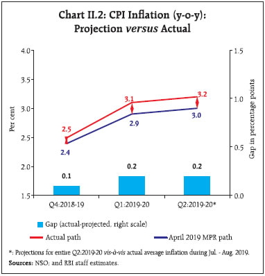
II. Prices and Costs Consumer price inflation registered an uptick during March-August 2019, underpinned by a pick-up in food inflation, particularly in vegetables and protein-based items. Fuel group inflation moderated sequentially after April and moved into deflation in July and August 2019. Inflation excluding food and fuel has softened since March in a broad-based manner notwithstanding a sharp increase in gold prices. Nominal growth in rural wages, both for agricultural and non-agricultural labourers, remained subdued. Growth in organised sector staff costs showed divergent movements – rising for the manufacturing sector and remaining range bound for the services sector. Farm inputs and industrial raw materials price inflation has softened in 2019-20 so far. Over the last six months i.e., March-August 2019 consumer price index (CPI) inflation trailed below the target of 4.0 per cent averaging 3.1 per cent over this period.1 Its key driver was food prices which emerged out of deflation in March 2019 and gradually firmed over the ensuing months in the usual summer season upturn. In contrast, prices of fuel and light items remained soft and slumped into deflation during July-August 2019. Excluding food and fuel, inflation ebbed by around 100 basis points between March- June 2019 and reached a 23-month low in June 2019, before registering some uptick during July-August (Chart II.1). The RBI Act, 1934 (amended in 2016) enjoins the RBI to set out deviations of actual outcomes from projections, if any, and to explain the underlying reasons thereof. The Monetary Policy Report (MPR) of April 2019 had projected CPI inflation at 2.9 per cent for Q1:2019-20 and 3.0 per cent for Q2:2019-20. Actual inflation outcomes have, by and large, tracked these projections (Chart II.2). While food prices moved out of deflation as anticipated, the summer rise in prices of vegetables this year was more pronounced than observed in recent history. Pulses prices moved out of two and a half years of deflation in May 2019. As a result, food inflation inched up by 230 basis points, larger than expected, between March and August 2019. Meanwhile, inflation excluding food and fuel softened more than anticipated, providing an offset. The Indian basket of crude oil prices eased unexpectedly – from an average of US$ 67 per barrel during 2019-20 (which was the baseline assumption in the April MPR) to below US$ 60 per barrel in August. Prices within the fuel group underwent substantial correction in respect of both rural items of consumption such as firewood and dung cake and those of urban usage such as liquefied petroleum gas (LPG). Consequently, the fuel group as a whole slipped into deflation during July-August. On the whole, these divergent movements caused CPI headline inflation outcomes to marginally overshoot inflation projections, i.e., by 20 basis points each in Q1:2019-20 and Q2:2019-20 (July-August) (Chart II.2). 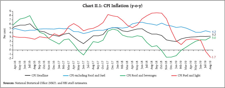
 II.1 Consumer Prices A decomposition of year-on-year (y-o-y) inflation shows that its rising trajectory during March to June 2019 was propelled by a sustained increase in price momentum (Chart II.3). In July, large favourable base effect helped moderate the high price momentum.2 In August, however, the price momentum outweighed a low base effect and consequently, inflation edged up marginally. The elevation in price momentum in H1:2019-20 was driven by the food group, mainly by prices of vegetables, pulses, meat and fish. In contrast, the momentum underlying fuel and light inflation collapsed during July-August under the weight of a broad-based decline in prices of items of rural and urban fuel consumption. The momentum of prices of items excluding food and fuel moderated during March-August 2019 and was completely overwhelmed by favourable base effects, barring July. The distribution of inflation across CPI groups shows a considerable drop in median inflation rates – from 4.8 per cent in 2018 to 2.1 per cent in 2019 so far. Moreover, the negative skew in inflation in 2017 and 2018 resulting from food prices was absent in 2019, implying that a generalised moderation in inflation was underway this year (Chart II.4). Diffusion indices of month-on-month (m-o-m) price changes in CPI items on a seasonally adjusted basis moderated during June-August 2019 across both goods and services categories (Chart II.5).3
II.2 Drivers of Inflation A historical decomposition of inflation shows that it was impacted by positive supply shocks in H1:2019- 20, which, in conjunction with subdued domestic demand, kept headline inflation low and stable (Chart II.6a).4 The break-up of overall CPI inflation into goods and services components suggests that perishable goods (non-durable goods with 7-day recall) such as vegetables and fruits were the largest contributor to overall inflation during April-August (Chart II.6b). The contribution of less perishable goods (non-durable goods with 30-day recall) moderated due to deflation in prices of rice, petroleum products, LPG and electricity. The contribution of durable goods to overall inflation increased during June-August 2019, primarily on account of a sharp increase in prices of gold and to a lesser extent, in those of motor vehicles. Imported goods (petrol; diesel; LPG; kerosene; electronic goods; gold; silver; chemical and chemical products; metal and metal products; and refined vegetables oils) together contributed negatively to overall inflation in the recent period (Chart II.6c). The contribution of services to overall inflation moderated. However, services (with a weight of 23.4 per cent in overall CPI) contributed to about a third to overall inflation (Chart II.6b). CPI Food Group In terms of weighted contribution, the food and beverages group (weight: 45.9 per cent in CPI) contributed 32.9 per cent to overall inflation during April-August 2019 as compared with 25.0 per cent for the same period a year ago. Inflation in the food group turned positive beginning March 2019 – after remaining in the negative zone for five consecutive months during October 2018-February 2019 – and increased steadily thereafter driven by prices of vegetables, fruits and protein-rich items such as pulses, meat, fish and milk (Chart II.7a). Within the food and beverages group, the price build-up during the financial year so far in the case of vegetables has been substantial, but close to historical summer price increases. In the case of fruits, pulses, meat and fish, the price build-up has been, in fact, larger than the historical average (2011-18). For all the other sub-groups within the food group, the build-up has been much lower than in the past (Chart II.7b).  Inflation in respect of cereals (weight of 9.7 per cent in CPI and 21.1 per cent in the food and beverages group) remained moderate during April-August 2019, with rice prices remaining in deflation, reflecting robust production and adequate stocks. As per the fourth advance estimates of foodgrain production, production of rice was at 1164 lakh tonnes in 2018- 19, higher than 1128 lakh tonnes in 2017-18, which was until recently an all-time record. Exports of rice declined during April-July 2019 as the 5 per cent incentive provided by the government to rice exporters under the Merchandise Exports from India Scheme (MEIS) was withdrawn from April 1, 2019 and this resulted in higher domestic availability. Wheat inflation, however, remained high at an average of 6.8 per cent during April-August 2019 (3.4 per cent in 2018-19) due to a fall in imports following a hike in import duty to 40.0 per cent in April 2019 from 30.0 per cent in May 2018. As regards vegetables (weight of 6.0 per cent in CPI and 13.2 per cent in the food and beverages group), a recovery in the prices of onions, tomatoes and potatoes (which account for 36.5 per cent of the total CPI vegetables) led the upturn in prices (Chart II.8a). Potato price pressures picked up right from April 2019. First, untimely rains during February and March in West Bengal impacted the crop which was ready to be harvested. Second, mandi arrivals declined due to a sudden increase in temperature during summer months and thunderstorms in several parts of northern and north-eastern states that spoiled the produce in transit. Despite this firming up, potato prices moved into deflation beginning April 2019 on account of favourable base effects. Onion prices, which had declined during December 2018-March 2019, revived from April with a sharp uptick during June-August. A reduction in rabi onion acreage in Maharashtra, particularly in the major onion-producing district of Nashik due to drought-like conditions, led to a slump in mandi arrivals. Onion prices were also supported by procurement operations by the National Agricultural Cooperative Marketing Federation of India (NAFED) in Maharashtra. Excessive rainfall, coupled with floods in several parts of major onion-supplying states such as Maharashtra, Karnataka and Madhya Pradesh during July-August, also led to a reduction in supplies. Tomato prices began picking up from March 2019, with inflation in this item rising sharply to 70.1 per cent in May 2019 from (-) 52.2 per cent in November 2018. Delayed harvesting in Maharashtra as well as fungus damaged crops in Karnataka triggered the initial uptick in prices, which was exacerbated by supply disruptions due to incessant rains and floodlike situations in key supplier states – Karnataka, Maharashtra and Himachal Pradesh. Tomato inflation, however, eased to 28.4 per cent in July largely due to a favourable base effect, before hardening to 39.4 per cent in August on account of an adverse base effect. 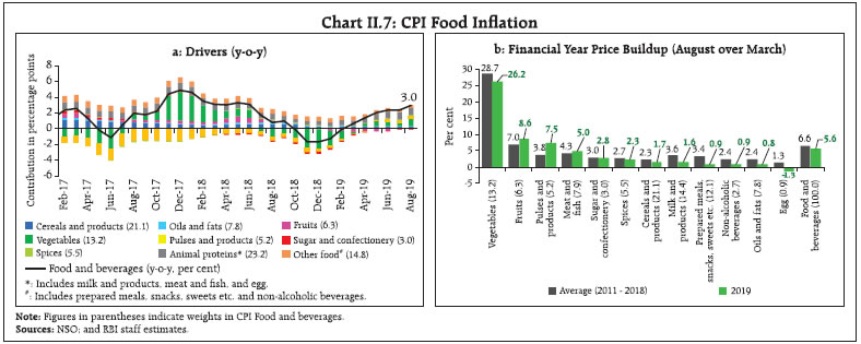 A decomposition of CPI vegetables into trend, cyclical and seasonal components reveals that the cyclical upswing, starting from December 2018, was the key driver of the vegetables inflation during H1:2019-20 (till July 2019), with the trend component remaining flat. The seasonal uptick during the summer season tracked the pattern in previous years (Chart II.8b). Prices of fruits (weight of 2.9 per cent in CPI and 6.3 per cent within the food and beverages group) moved into deflation in December 2018. Fruits prices began rising from February 2019 with sharp uptick in April and July. However, fruits remained in deflation up to August 2019. Price pressures were particularly evident in respect of bananas and apples, which together constitute around 35.6 per cent of the category of fruits. While banana prices were impacted by lower mandi arrivals, apple prices increased in the usual seasonal upturn. Apple prices were also supported by lower imports following the increase in import duty on apples from the US by 20.0 per cent in June 2019. However, price pressures in respect of both bananas and apples declined in August due to higher domestic arrivals in mandis. The rise in prices of vegetables and fruits during the summer months of 2019 was witnessed in urban as well as rural areas. A sectoral analysis suggests that there is no statistically significant difference between the m-o-m changes in prices of fruits and vegetables between rural and urban areas. There is, however, statistically significant higher volatility in m-o-m changes in prices of vegetables and fruits in urban areas than in rural areas5. CPI pulses (weight of 2.4 per cent in CPI and 5.2 per cent in the food and beverages group), driven by a sustained uptick in prices, emerged from 29 successive months of deflation in May 2019 to reach a 35-month high inflation of 6.9 per cent in August 2019 (Chart II.9a). Even so, the CPI pulses index remained below trend (Chart II.9b). Pulses production was lower at 234 lakh tonnes (as per the fourth advance estimates) in 2018-19 than 254 lakh tonnes in 2017-18. In addition, pulses imports declined from 57 lakh tonnes in 2017- 18 to 26 lakh tonnes in 2018-19, reducing the domestic supply glut. A sizeable stock of pulses – at around 40 lakh tonnes – is available, which could be released in the market to contain price pressures. Meat and fish prices also contributed to the pick-up in food inflation, partly reflecting the sustained rise in feed prices, particularly of maize. In fact, inflation in meat and fish prices was the highest in 62 months in July 2019. While egg prices moved in line with their historical pattern, those of milk and products hardened during May-August 2019, primarily reflecting an increase in retail milk prices by ₹2 per litre to ₹6 per litre due to pass-through of an increase in procurement prices of milk by ₹5-6 per litre by milk co-operatives.  Prices of sugar emerged out of deflation in May 2019 after remaining in negative territory for 15 consecutive months. However, they slipped back into deflation during June-August 2019, reflecting domestic supply surpluses as well as favourable base effects. As per the Indian Sugar Mills Association (ISMA), the opening stock of sugar as on October 1, 2019 is expected to be at an all-time high of 145 lakh tonnes. International sugar prices, which were in deflation during May 2017-February 2019 due to persistent excess global supply, also returned to positive territory in March 2019. Some increase in sugar prices in the domestic market was observed in Q1:2019-20, possibly reflecting the increase in minimum selling prices of sugar by ₹2 per kilogram in February 2019. Inflation in respect of oils and fats remained subdued at around 0.8 per cent during April-August 2019, with soft international prices and higher domestic production keeping prices under check. According to the fourth advance estimates, oilseeds production increased by 2.5 per cent in 2018-19; however, a decline in groundnut production during the year contributed to price pressures in groundnut oil during a major part of 2018-19 as well as in 2019-20 so far. CPI Fuel Group Fuel group inflation moderated sequentially after April up to June and sank into deflation in July and August 2019, with inflation in major constituents such as electricity, LPG, firewood and chips and dung cake all slipping into negative territory (Chart II.10a). 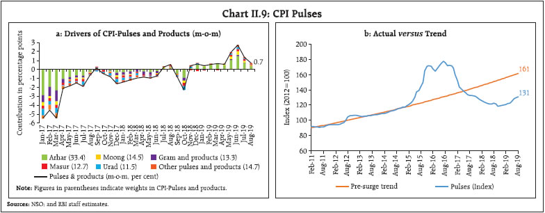
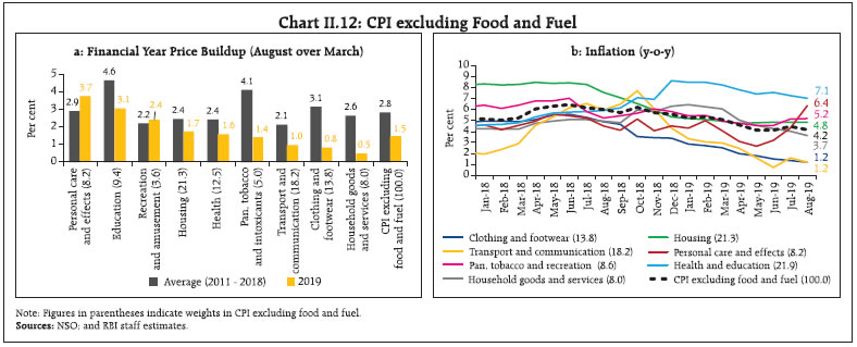
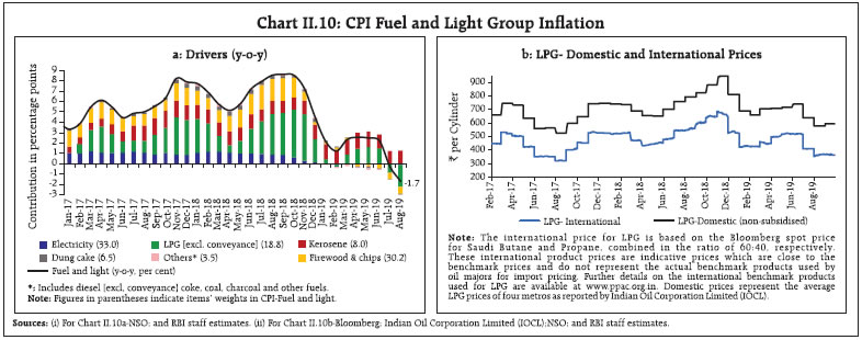 After registering price increases between March- June, domestic LPG prices declined abruptly in July and August, following a collapse in international petroleum products prices (Chart II.10b). Electricity prices, which constitute around one-third of the fuel and light sub-group, have been in deflation for most of the months since January 2019. Prices of items of rural consumption such as firewood and chips, and dung cake have also remained in deflation since April 2019. This could partly be on account of increased LPG use in rural areas.6 In contrast, administered kerosene prices registered calibrated increases as oil marketing companies (OMCs) raised administered prices to align them more closely with market prices so as to eventually phase out the subsidy on petroleum products. CPI excluding Food and Fuel CPI inflation excluding food and fuel moderated by close to 100 bps between March and June 2019. Even excluding volatile components such as petroleum products, gold and silver, it moderated by around 70 bps, reflecting the broad-based nature of the disinflation in this group. Although inflation excluding food and fuel picked up by 35 bps in July 2019, it was not sustained and it moderated by about 30 bps in August (Chart II.11). Within CPI excluding food and fuel, price increases during the financial year so far have been considerably lower than historical averages for most of the constituent sub-groups (Chart II.12). Empirical evidence suggests that persistently low food inflation has spilled over to CPI excluding food and fuel (Box II.1). 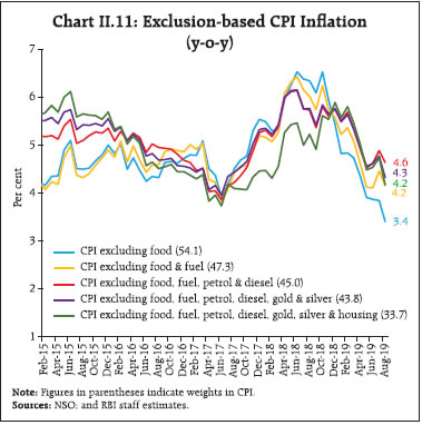
 Box: II.1: Time-varying Estimates of Spillovers from Food Inflation to Inflation excluding Food and Fuel 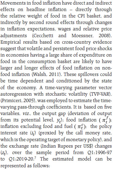
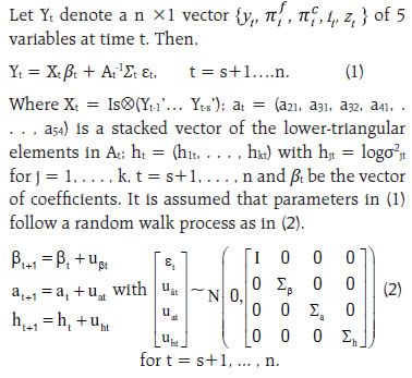
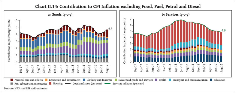
The empirical results suggest that (i) pass-through coefficients are time varying – ranging between 8 per cent and 14 per cent during Q3:2003-04 to Q1:2019- 20; (ii) pass-through is high when food inflation is high and persistent, and low when food inflation is low. In the recent low food inflation scenario, the pass-through coefficient has moderated to around 10 per cent (Chart II.1.1a & b). In view of this asymmetric impact of food inflation on inflation excluding food and fuel, maintaining low and stable food prices becomes critical to contain underlying inflation pressures. This would entail supply side reforms to ensure that food inflation remains under check. Reference Bordoloi, S. (2019), “Spill-over from Food inflation to Core inflation in India: An Empirical Analysis”, (Mimeo). Cecchetti, S. and Moessner, R. (2008), ‘Commodity prices and inflation dynamics’, Bank for International Settlements Quarterly Review, Bank for International Settlements, pp. 55–66. Reserve Bank of India (2014), ‘Report of the Expert Committee to Revise and Strengthen the Monetary Policy Framework (Chairman: Dr Urjit R. Patel)’. Primiceri, G. (2005), ‘Time Varying Structural Vector Autoregressions and Monetary Policy’, Review of Economic Studies, 72, pp. 821-852. Walsh, J. (2011), ‘Reconsidering the role of food prices in inflation’, IMF Working Paper, WP/11/71, International Monetary Fund. | Inflation in the transport and communication sub-group moderated primarily due to a sustained deflation in petroleum product prices (Chart II.13a). However, the wedge between international and domestic prices remains considerable due to an incomplete passthrough (Chart II.13b). An examination of the components of CPI excluding food, fuel, petrol and diesel inflation in terms of goods and services shows that while goods inflation saw phases of both moderation (February-May) and uptick (June-August), services inflation has fallen persistently (Chart II.14a & b). A key sub-group contributing to the downturn in goods inflation was clothing and footwear, mainly in rural areas. Other sub-groups contributing to the goods moderation were personal care items, particularly, gold; silver; and toiletries, and household goods and services items. The pick-up in goods inflation since June has almost entirely emanated from the personal care and effects sub-group, driven by a sharp pick-up in gold prices. Services inflation moderated from elevated levels in February 2019 to 4.9 per cent in August 2019 (Chart II.14b) in a broad-based manner across education services like tuition and coaching; transportation fares, particularly, bus fares; medical services; housing; and household services like sweeping and tailoring charges. 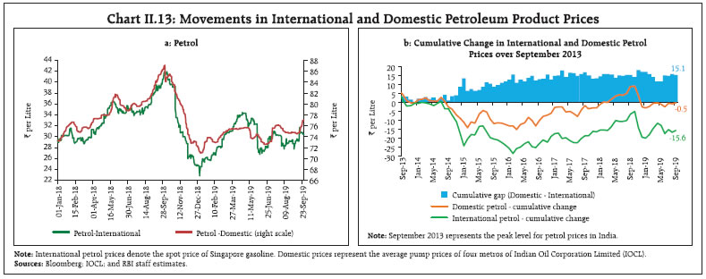
 Other Measures of Inflation Inflation in sectoral CPIs, i.e., for industrial workers (CPI-IW), agricultural labourers (CPI-AL) and rural labourers (CPI-RL), rose rapidly between March and June 2019 compared with the muted uptick in CPI headline inflation. Inflation in food and fuel components of CPI-AL and CPI-RL was higher than that in headline CPI and was accentuated by the larger share of food in these indices. In the case of CPI-IW, a major source of divergence was the housing component. Following the increase in HRA under the 7th central pay commission (CPC), housing inflation in CPI-IW remained above 26 per cent during July 2018 to June 2019, pushing CPI-IW inflation to 8.7 per cent by May 2019. As the effect of increase in HRA waned, CPI-IW inflation declined to 6.3 per cent in August. Inflation in wholesale price index (WPI) fell steadily in contrast to the sectoral CPIs to a low of 1.1 per cent in August 2019. On the one hand, fuel group inflation collapsed from 4.6 per cent in March to (-) 4.0 per cent in August 2019 tracking international petroleum product prices; inflation in non-food manufactured products also fell across the board and was in contraction in August. On the other hand, WPI food inflation showed an uptick from January and remained elevated till August, barring a fleeting correction in July. GDP and GVA deflators broadly remained in alignment with CPI inflation during the last six months (Chart II.15a). Underlying inflation dynamics can be gauged from exclusion-based measures that remove volatile items/item groups or by statistical measures such as trimming, which adjust for positive and negative skewness and chronic fat tails in the inflation distribution by removing outliers. By these measures, inflation have moved with a softening bias over the last six months (Chart II.11 & 15b). II.3 Costs Developments in underlying cost conditions have largely been in sync with inflation in terms of the WPI (Chart II.16). Price inflation in farm inputs and industrial raw materials (extracted from the WPI) has fallen in 2019-20 so far. The moderation in global crude oil prices during 2019-20 has kept domestic price pressures under check in respect of inputs such as high-speed diesel, aviation turbine fuel, naphtha, furnace oil and petroleum coke. In addition, the contraction in mineral prices has also aided the fall in industrial input costs. Among other industrial raw materials, domestic coal inflation has subsided significantly since the beginning of 2019-20, averaging around 0.7 per cent during April-August 2019. Domestic coal prices largely moved in line with international coal prices during the period. Inflation in paper and paper products has also moderated due to lower raw material costs including those of pulp and coal. In the case of fibres, inflation eased during June-August 2019, predominantly reflecting the easing in prices of raw jute and raw cotton. Of farm sector inputs, price pressures in respect of fertilisers remained subdued, largely reflecting moderation in international prices, especially those of phosphate, di-ammonium phosphate and triple superphosphate. Inflation in respect of pesticides and other agrochemical products also softened considerably in Q1:2019-20 due to easing of international crude oil prices. The price of electricity, which carries a high weight in both industrial and farm inputs, moved into deflation during June-August 2019. However, inflation in fodder prices turned positive in January 2019, after remaining in deflation during August 2016-December 2018 (barring August 2017), to touch a 37-month high of 16 per cent in July 2019, before easing somewhat in August. Inflation in terms of agricultural machinery and implements costs has also remained elevated and sticky from H2:2018-19. Growth in nominal rural wages, both for agricultural and non-agricultural labourers, remained subdued and sticky, hovering around 3.7 per cent and 3.8 per cent, respectively, during 2019-20 so far, reflecting the lagged impact of moderate rural inflation, low food prices and a slowdown in the construction sector (Chart II.17).
With inflation in CPI-AL and CPI-RL having picked up since February 2019, however, real rural wage growth, based on these price indices, turned negative since March 2019. Growth in organised sector staff costs showed divergent movements for services and manufacturing firms. Unit labour costs for companies in the manufacturing sector fell marginally in Q4:2018-19 but rose thereafter in Q1:2019-20 to 6.3 per cent due to a decline in the value of production, coupled with increase in staff cost.8 Unit labour cost for firms in the services sector increased marginally in the last quarter as higher growth in staff costs outpaced the growth in value of production (Chart II.18). Manufacturing firms participating in the Reserve Bank’s industrial outlook survey reported a fall in input costs in Q2:2019-20 on account of lower raw material costs. The cost of finance and salary outgoes are also expected to soften in Q2. The fall in input prices is likely to translate into a fall in selling prices in Q2. Firms polled for the manufacturing purchasing managers’ index (PMI) reported a decline in input costs and selling prices sequentially from Q2:2018-19 to Q1:2019-20. However, the rate of decline in selling prices in Q1:2019-20 was sharper than that of input costs. During Q2:2019-20, both input costs and selling prices firmed up. Input cost inflation reported by firms in the services sector PMI also softened gradually from Q2:2018-19 to Q1:2019-20 but increased during the first two months of Q2:2019-20. II.4 Conclusion The inflation trajectory in 2019-20 so far has been characterised by rising food inflation, with price build-ups close to historical averages and well above levels observed in recent years, driven largely by a strong summer pick-up in prices of vegetables. Going forward, however, the build-up in vegetables prices is likely to reverse with arrivals of the kharif harvest and winter supplies. The catch-up in monsoon and sowing should help mitigate price pressures in cereals. Moreover, buffer stocks of cereals are well above prescribed norms. In the case of pulses, the arrival of fresh produce in the market along with buffer stocks are also likely to keep prices under check. Going forward, domestic fuel and petroleum product prices are subject to considerable uncertainty due to geopolitical developments in the Middle East. A sudden spike in crude oil and petroleum products prices remains a major upside risk in spite of weak global demand. However, given the weak domestic demand and lower input costs, inflation in CPI excluding food and fuel is likely to remain moderate. Forward looking surveys of the Reserve Bank point to weak consumer confidence and sagging demand, especially pertaining to non-essential items. Manufacturing firms see input prices as still soft and pricing power is yet to firm up as the cost of finance and salary outgoes remain muted. However, inflation expectations of households have risen somewhat. On the whole, headline CPI inflation is expected to remain within the Reserve Bank’s target of 4.0 per cent during 2019-20. _________________________________________________________
III. Demand and Output Aggregate demand weakened in Q1, underpinned by a slowdown in private consumption. On the supply side, a sharp deceleration in manufacturing essentially reflected weaknesses in the organised sector. Services sector growth was pulled down by ‘financial, real estate and professional services’ and construction activity. The recent measures by the Government should help kickstart the capex cycle and lead to the strengthening of domestic demand. Domestic economic activity suffered a sharp loss of pace in Q1:2019-20. Aggregate demand weakened in Q1:2019-20 by a slowdown in private consumption. On the supply side, manufacturing activity collapsed with the prolonged slowdown in the production of capital goods and consumer durables and in the services sector, construction activity slowed down markedly. Incoming data suggest that the slowdown persisted into Q2:2019-20. III.1 Aggregate Demand Measured by year-on-year (y-o-y) changes in real gross domestic product (GDP) at market prices, the deceleration in aggregate demand in Q4:2018-19 deepened to 5.0 per cent in Q1:2019-20, extending the sequential slowdown that set in during Q1:2018- 19 to the fifth consecutive quarter (Table III.1 and Chart III.1a). Momentum, measured by quarter-onquarter (q-o-q) seasonally adjusted annualised GDP growth rate (SAAR), also moderated to 4.4 per cent in Q1:2019-20 from 5.6 per cent in Q4:2018-19 (Chart III.1b). Of the constituents of GDP, private final consumption expenditure (PFCE), the mainstay of aggregate demand, slumped, with its growth plummeting by over four percentage points in Q1:2019-20 to an eighteen-quarter low. Government final consumption expenditure (GFCE) cushioned the deceleration in aggregate demand. Excluding GFCE, real GDP growth would have slid down to 4.5 per cent in Q1:2019- 20. Gross fixed capital formation (GFCF) remained weak in Q1:2019-20, with the capex cycle yet to gain traction. Export growth decelerated considerably in Q1:2019-20 in an uncertain external trading environment rendered hostile by trade tensions. With import growth reflecting domestic demand conditions and slowing more sharply, net exports made a positive contribution to growth after a gap of nine quarters. | Table III.1: Real GDP Growth (Per cent) | | Item | 2017-18 (FRE) | 2018-19 (PE) | Weighted Contribution* | 2017-18 (FRE) | 2018-19 (PE) | 2019-20 | | 2017-18 | 2018-19 | Q1 | Q2 | Q3 | Q4 | Q1 | Q2 | Q3 | Q4 | Q1 | | Private final consumption expenditure | 7.4 | 8.1 | 4.2 | 4.5 | 10.1 | 6.0 | 5.0 | 8.8 | 7.3 | 9.8 | 8.1 | 7.2 | 3.1 | | Government final consumption expenditure | 15.0 | 9.2 | 1.5 | 1.0 | 21.9 | 7.6 | 10.8 | 21.1 | 6.6 | 10.9 | 6.5 | 13.1 | 8.8 | | Gross fixed capital formation | 9.3 | 10.0 | 2.9 | 3.1 | 3.9 | 9.3 | 12.2 | 11.8 | 13.3 | 11.8 | 11.7 | 3.6 | 4.0 | | Exports | 4.7 | 12.5 | 1.0 | 2.5 | 4.9 | 5.8 | 5.3 | 2.8 | 10.2 | 12.7 | 16.7 | 10.6 | 5.7 | | Imports | 17.6 | 15.4 | 3.8 | 3.6 | 23.9 | 15.0 | 15.8 | 16.2 | 11.0 | 22.9 | 14.5 | 13.3 | 4.2 | | GDP at Market Prices | 7.2 | 6.8 | 7.2 | 6.8 | 6.0 | 6.8 | 7.7 | 8.1 | 8.0 | 7.0 | 6.6 | 5.8 | 5.0 | FRE: First Revised Estimates; PE: Provisional Estimates.
*: Component-wise contributions to growth do not add up to GDP growth in the table because change in stocks, valuables and discrepancies are not included.
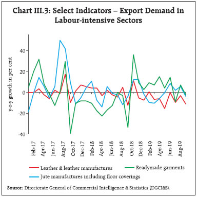
Source: National Statistical Office (NSO), Government of India. | GDP Projections versus Actual Outcome The April 2019 MPR had projected real GDP growth of 6.8 per cent for Q1:2019-20, with risks evenly balanced around the baseline path (Chart III.2). The actual outcome for the quarter undershot the projections by 180 basis points. First, the realised growth in private consumption demand surprised significantly on the downside, indicating that the April 2019 projection underestimated the broad-based slowdown in both rural and urban consumption. Second, GFCF growth also turned out lower than the projection on account of lower than expected capital goods production and their imports, and moribund activity in construction. III.1.1 Private Final Consumption Expenditure The unexpected slump in PFCE resulted in its share falling to 55.1 per cent in Q1:2019-20 from 56.1 per cent a year ago. The slowdown in private consumption was amplified by weak growth in some of the labour intensive export sectors such as readymade garments, leather manufactures and jute manufactures (Chart III.3). 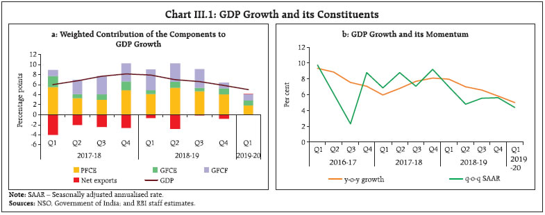

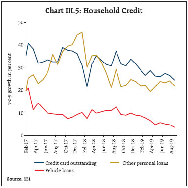
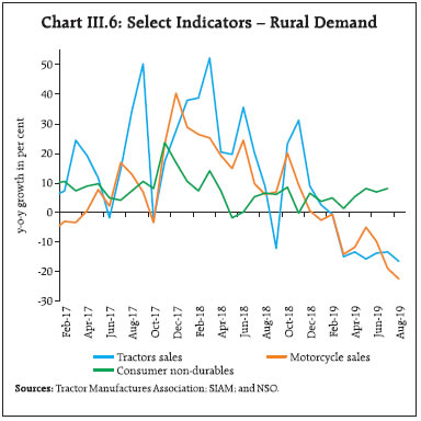
 High frequency indicators of urban demand have weakened in recent months as reflected in contraction in sales of passenger vehicles and production of consumer durables (Chart III.4). Among them, passenger car sales have contracted by double digits every month since April 2019, resulting in major car producers suspending factory production intermittently. A combination of factors such as higher prices due to stricter safety norms, uncertainty caused by new emission norms and the proposed switching to electric vehicles have dented the sales of passenger vehicles (Box III.1). The growth in household credit for vehicles extended by banks also moderated (Chart III.5). Domestic air passenger traffic growth remained modest in July due to grounding of a private airline, which impacted air fares and dampened demand; however, it improved in August. Going forward, passenger vehicle sales could improve with the government’s recent support for the sector such as permitting the operation of Bharat Stage (BS)-IV vehicles purchased till March 31, 2020, for the entire period of registration; withdrawal of a ban on the purchase of new vehicles by government departments; and deferring the implementation of hike in the one-time registration fee until June 2020. Various indicators of rural demand have also remained weak (Chart III.6). Motorcycles and tractor sales contracted in July and August. Although the growth of consumer non-durables accelerated in July, it was driven mainly by sunflower oil. The sales growth of fast moving consumer goods (FMCG) companies, a sizeable part of which occurs in rural areas, has also been sluggish. The reasonably strong kharif foodgrains production in the first advance estimates of the Ministry of Agriculture – only 0.8 per cent below last year’s level – and bright prospects for the rabi season in view of soil moisture conditions and comfortable reservoir levels could buoy rural incomes and demand, going forward. 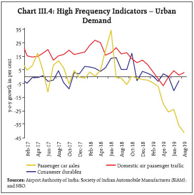
 Box III.1: Slowdown in the Automobile Sector The downturn in the automobile sector in India, which could be attributed to several regulatory and institutional factors, was accentuated by a slowdown in demand. This has drawn considerable attention in view of the industry’s role in economic activity1. An estimation framework using vector auto regressions with exogenous variables (Ludvigson, 1998) (VARX) was conducted to assess the underlying factors for the slump in the auto sector using quarterly data from Q1:2007-08 to Q1:2019- 20. In the first VARX (1): Y = A(L)Y + CX + U, ....(1) where Y = [ct, yt, st, it] is a vector of variables endogenous to the simultaneous system of equations. ct is the credit demand measured as a gap between the credit disbursed by scheduled commercial banks (SCBs) for automobile purchases from its long-term trend. st is the deviation of sales of commercial vehicles from its long-term trend. yt is aggregate demand measured as the output gap and it is the weighted average lending rate of SCBs. A rise in aggregate demand and credit demand are expected to increase vehicle sales. On the other hand, an increase in interest rate is expected to moderate auto sales. X = [zt, pt, d1, d2] is a vector of exogenous variables determined from outside the simultaneous system of equations, zt is the y-o-y change in INR/US$ exchange rate, pt is the y-o-y change in diesel prices, d1 is a dummy variable representing the implementation of BS-IV from April 2017. d2 is a dummy variable representing three events which happened during the second half of 2018-19, viz., liquidity issues faced by non-banking financial companies (NBFCs) post-IL&FS default, the announcement of axle load norms and implementation of insurance and safety norms. Ut is a vector of idiosyncratic errors. A similar model was estimated by using the deviation of sales of passenger cars from its long-term trend instead of sales of commercial vehicles (st) in (1). The key findings emerging from the impulse response functions (IRFs) from the two VARXs (Charts III.I.1) are:
(i) both commercial vehicle and passenger car sales are sensitive to aggregate demand shocks; (ii) both commercial vehicle and passenger car sales respond positively to a decline in interest rates; (iii) fuel prices have a negative impact on commercial vehicle sales; (iv) exchange rate depreciation affects auto sales negatively; and (v) bank credit does not have any significant impact on vehicle sales; however, the reverse causation is statistically significant, i.e., sales of commercial vehicles positively impact bank credit flow to the automobile sector. The dummy, representing three events (d2) is statistically significant and explains 10 percentage points of the decline in commercial vehicle sales and 8 percentage points of the decline in passenger car sales. Shocks like the slump in demand, liquidity crisis in the NBFC sector and measures to enhance safety and security norms, appear to have resulted in a downswing in the automobile sector. A slowdown in passenger car sales was also observed in the US, the Euro area, China, South Korea and Japan for a variety of reasons (Chart III.1.2). These are: (i) stricter emission norms in China and the Euro area; (ii) mandatory sales of electric vehicles by car makers in the Euro area; (iii) tepid demand due to subdued global growth; and (iv) depressed consumer confidence from escalating US-China trade tensions. Reference: Ludvigson, S. (1998). “The Channel of Monetary Transmission to Demand: Evidence from the Market for Automobile Credit”, Journal of Money, Credit and Banking, 30(3), pp. 365–383. | III.1.2 Gross Fixed Capital Formation Growth in gross fixed capital formation (GFCF) moderated sharply in Q4:2018-19 and Q1:2019-20 after double digit growth in the five previous quarters. The share of GFCF in aggregate demand declined to 32.5 per cent in Q1:2019-20 from 32.8 per cent a year ago. High frequency indicators suggest that investment activity remained sluggish in Q2. Import of capital goods and production of capital goods contracted in July (Chart III.7). However, housing loans disbursed by scheduled commercial banks (SCBs) remained resilient, reflecting the policy push for the affordable housing sector. Capacity utilisation (CU) in the manufacturing sector, measured by the order books, inventory and capacity utilisation survey (OBICUS) of the Reserve Bank, moderated to 73.6 per cent in Q1:2019-20 from 76.1 per cent in Q4:2018-19; seasonally adjusted CU, however, improved to 74.8 per cent in Q1:2019-20 from 74.5 per cent in Q4 (Chart III.8). The number of stalled projects in the private sector declined in Q1:2019-20, while there was some deterioration in stalled projects in the government sector in Q1 (Chart III.9). Gross capital formation has decelerated since 2011-12 due to a slowdown in investment by the private sector (Chart III.10). Underlying the latter is corporate deleveraging in select industries as reflected in improving interest coverage ratios (Chart III.11). The slowdown in investment activity was also reflected in a decline in financial flows from banks and non-banks to the commercial sector (Chart III.12; see Chapter IV for details).
III.1.3 Government Expenditure Government final consumption expenditure (GFCE) cushioned aggregate demand in Q4:2018-19 and Q1:2019-20, as pointed out earlier. During April-August 2019, the fiscal position of the central government strengthened as the gross fiscal deficit (GFD) and revenue deficit (RD) improved vis-à-vis the corresponding period of the previous year in terms of budget estimates (BE), mainly due to lower growth in expenditure (Table III.2). Total expenditure of the central government in the current fiscal year so far has been driven by revenue expenditure. 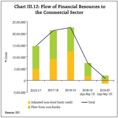 | Table III.2: Key Fiscal Indicators – Central Government (April-Aug) | | (Per cent) | | Indicator | As a per cent of BE | y-o-y Growth | | 2018-19 | 2019-20 | 2019-20 | | 1. Revenue receipts | 26.9 | 30.7 | 29.8 | | a. Tax revenue (Net) | 24.7 | 24.5 | 10.5 | | b. Non-tax revenue | 40.1 | 63.4 | 102.0 | | 2. Total non-debt receipts | 26.4 | 29.8 | 29.6 | | 3. Revenue expenditure | 43.8 | 42.5 | 10.7 | | 4. Capital expenditure | 44.0 | 40.2 | 3.0 | | 5. Total expenditure | 43.8 | 42.2 | 9.8 | | 6. Gross fiscal deficit | 94.7 | 78.7 | -6.3 | | 7. Revenue deficit | 114.0 | 89.9 | -8.1 | | 8. Primary deficit | 767.7 | 773.4 | -10.0 | BE: Budget Estimates.
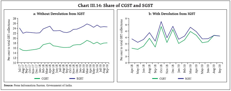
Sources: Controller General of Accounts; and Union Budget Document, 2019-20. | In order to meet expenditure commitments, revenue generation is critical. On the receipts side, income tax collections gained traction during April-August 2019 (Chart III.13). Notwithstanding month-over-month fluctuations, the GST collections grew by 4.9 per cent (y-o-y) during April-September 2019. The share of State GST (SGST) collections in total GST revenue has been sizably higher than Central GST (CGST), attributable to the adjustment for input tax credit. After apportionment of integrated GST (IGST) collections, the share of CGST collections remained significantly lower than SGST collections during April-September 2018. They did move closer subsequently, before finally catching up in August 2019 (Chart III.14a and 14b). There have, however, been large inter-state variations in SGST collections, with a few states not requiring the GST compensation cess. Plugging loopholes and mitigating information technology (IT) glitches such as putting in place an invoice-matching system to facilitate a system validated input tax credit, overcoming operational deficiencies of the payment module, alignment of system validations with the GST Acts and Rules along with alleviating system design deficiencies may facilitate tapping of GST potential.2 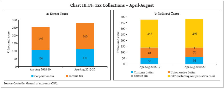
 Non-tax revenue has been an important source of finance for the central government. During April- August 2019, this component witnessed robust growth driven by the surplus transfer from the Reserve Bank. Resource mobilising efforts through disinvestment may also help garner revenues, going forward. On the expenditure front, both revenue and capital expenditure of the central government witnessed some moderation in Q1:2019-20. However, after the declaration of election results, both revenue and capital expenditure picked up significantly during July-August 2019; almost 40 per cent of budgeted capital expenditure for roads and highways was incurred in the month of July 2019. Likewise, information available for 22 states indicates a slowdown in revenue expenditure in Q1:2019-20 though it picked up in July 2019. States have reduced their capital spending in order to adhere to fiscal deficit targets in the last few years (Chart III.15). This seems to have, in turn, affected investment adversely. Going forward, a pick-up in capital spending by both the centre and states is desirable given the growth augmenting property of the capital expenditure multiplier (RBI, 2019).3 A major challenge for government finances in the remaining period of the current financial year is to adhere to the budgeted capital spending and revenue generation targets. As regards direct taxes of states, stamp duty collections are highly correlated with construction activity (Chart III.16). Hence, a slowdown in the construction sector might impact stamp duty collections.
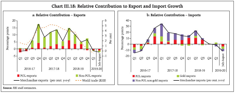
After remaining above 6 per cent of GDP between 2008-09 to 2016-17, the combined GFD of the centre and states dropped below 6 per cent in 2017-18. It is estimated at 6.2 per cent in 2018-19 (RE) and 5.9 per cent in 2019-20 (BE). Outstanding liabilities of the general government are budgeted to marginally decline to 69.6 per cent of GDP in 2019-20 from 69.8 per cent in 2018-19, driven by the centre, though states’ debt is showing a rising trend. The debt servicing capacity of the general government has improved in 2018-19 with the interest payments as per cent to revenue receipts exhibiting a decline. The Reserve Bank has managed the centre’s market borrowing programme during 2019-20 so far as per the planned issuance schedule. The budgeted gross market borrowing of the central government for 2019-20 at ₹7,10,000 crore is about 24.3 per cent higher than last year. The central government completed 62.3 per cent of its budgeted gross market borrowings as on September 30, 2019 (50.4 per cent in the corresponding period of 2018-19) (Table III.3). The Union Budget 2019-20 provides for consolidation measures like switching of securities budgeted at ₹50,000 crore, of which ₹40,109 crore worth of securities have already been switched. The states completed 35.6 per cent of their budgeted gross market borrowings till September 30, 2019 as compared with 27.6 per cent in the corresponding period of 2018-19. A major part of market borrowings by the states is expected to occur in H2:2019-20. | Table III.3: Government Market Borrowings | | (₹ crore) | | Item | 2017-18 | 2018-19 | 2019-20 (September 30, 2019) | | Centre | States | Total | Centre | States | Total | Centre | States | Total | | Net borrowings | 4,48,410 | 3,40,281 | 7,88,691 | 4,22,737 | 3,48,643 | 7,71,380 | 3,40,972 | 1,56,447 | 4,97,419 | | Gross borrowings | 5,88,000 | 4,19,100 | 10,07,100 | 5,71,000 | 4,78,323 | 10,49,323 | 4,42,000 | 2,25,445 | 6,67,445 | III.1.4 External Demand Net exports contributed positively to aggregate demand in Q1:2019-20 for the first time after Q2:2016-17, as slowdown in import growth was more pronounced than that for exports. The persisting loss of momentum in global trade impacted India’s merchandise exports, which contracted during Q1:2019-20 and in July-August 2019-20 in both the petroleum, oil and lubricants (POL) and non-POL categories (Chart III.17a). The sectors which contributed to the overall decline included engineering goods, gems and jewellery and rice. POL exports declined mainly on account of a fall in international crude oil prices. In addition, routine maintenance-related shutdowns in major refineries adversely impacted exports in June 2019 (Chart III.18a). Imports also contracted in Q1:2019-20 due to deceleration in POL growth and decline in non-POL non-gold imports. Gold imports surged on the back of a decline in prices, wedding and festive season demand during Q1:2019-20 (Chart III.18b). The decline in non- POL non-gold imports was broad-based as imports of transport equipment, pearls and precious stones, metalliferous ores and vegetable oil contracted. Imports continued to contract in July-August 2019 in a broad-based manner. The trade deficit moderated from US$ 46.7 billion in Q1:2018-19 to US$ 46.2 billion in Q1:2019-20, although on a sequential basis, i.e., Q1:2019-20 over Q4:2018-19, it expanded modestly. However, with imports declining faster than exports, the trade deficit narrowed from US$ 36.5 billion in July-August 2018-19 to US$ 26.9 billion in the corresponding period of 2019-20. While the current account deficit (CAD) mirrored the movements in the trade deficit, both on a y-o-y and sequential basis, CAD as per cent of GDP widened to 2 per cent in Q1:2019-20 from below one per cent in Q4:2018-19. More than 80 per cent of the trade deficit was financed through invisibles, i.e., net export of services and remittances. Net services exports grew by 7.3 per cent in Q1:2019-20 on a y-o-y basis – primarily driven by software, travel and financial services (Chart III.17b). Revenue growth of major information technology (IT) companies making software exports, improved on a y-o-y basis in Q1:2019-20; an increase of 0.6 per cent in total global IT spending is projected in 2019. Remittances remained stronger in Q1:2019- 20, though the net outgo of payments under income account increased due to higher dividends on foreign investment in Q1:2019-20. The CAD was comfortably met by a mix of foreign direct investment (FDI), foreign portfolio investment (FPI) and external commercial borrowings in Q1:2019-20 with net accretion to reserves to the tune of US$ 14.0 billion. Higher FPI flows, including under the voluntary retention route (VRR) introduced in March 2019, eased external financing conditions. Net inflows under external commercial borrowings to India stood at US$ 6.3 billion in Q1:2019-20 as against an outflow of US$ 1.5 billion a year ago. Net FDI flows at US$ 13.9 billion in Q1:2019-20 were higher than US$ 9.6 billion a year ago. Easing of norms for FDI in single brand retail, contract manufacturing, and coal mining are likely to give a push to FDI inflows and strengthen India’s participation in the global value chain. Notwithstanding outflows from the equity segment in July and August 2019, net FPI purchases (excluding VRR) in the domestic capital market were at US$ 3.3 billion during April-September 2019 as against an outflow of US$ 11.5 billion a year ago. Net flows under non-resident deposits were robust in Q1:2019- 20. India’s forex exchange reserves were placed at US$ 434.6 billion on October 1, 2019 – an increase of US$21.7 billion over the level at end-March 2019. 
 III.2 Aggregate Supply On the supply side, the gross value added (GVA) growth decelerated to 5.7 per cent in Q4:2018-19 and further to a twenty-one-quarter low of 4.9 per cent in Q1:2019-20 (Table III.4). GVA momentum, measured in terms of seasonally adjusted q-o-q annualised growth, also declined sharply in Q1 (Chart III.19). The deceleration in GVA growth (y-o-y) was caused by a significant deceleration in services growth to 6.7 per cent in Q1:2019-20 from 8.2 per cent in Q4:2018- 19, pulled down by construction and ‘financial, real estate and professional services’. Manufacturing registered the second lowest growth in the 2011- 12 series4. Despite some deceleration, public administration, defence and other services (PADO) grew at a healthy rate. Excluding PADO, the GVA growth would have slipped to 5.0 per cent in Q4:2018- 19 and 4.5 per cent in Q1:2019-20 (Chart III.20). Growth in ‘trade, hotels, transport, communication and services related to broadcasting’ registered an uptick sequentially. III.2.1 Agriculture In Q1:2019-20, value added in agriculture and allied activities recovered from contraction in the preceding quarter on the back of higher production of wheat and oilseeds during the rabi season. This was also supported by higher horticulture production by 0.7 per cent to a record of 3,138 lakh tonnes, as per the third advance estimates for 2018-19. | Table III.4: Sector-wise Growth in GVA | | (y-o-y, per cent) | | Sector | 2017-18 (FRE) | 2018-19 (PE) | Weighted Contribution | 2017-18 (FRE) | 2018-19 (PE) | 2019- 20 | | 2017-18 | 2018-19 | Q1 | Q2 | Q3 | Q4 | Q1 | Q2 | Q3 | Q4 | Q1 | | Agriculture, forestry and fishing | 5.0 | 2.9 | 0.8 | 0.4 | 4.2 | 4.5 | 4.6 | 6.5 | 5.1 | 4.9 | 2.8 | -0.1 | 2.0 | | Industry | 6.1 | 6.2 | 1.4 | 1.4 | -0.1 | 7.7 | 8.0 | 8.6 | 9.9 | 6.1 | 6.0 | 3.4 | 1.7 | | Mining and quarrying | 5.1 | 1.3 | 0.2 | 0.0 | 2.9 | 10.8 | 4.5 | 3.8 | 0.4 | -2.2 | 1.8 | 4.2 | 2.7 | | Manufacturing | 5.9 | 6.9 | 1.1 | 1.2 | -1.7 | 7.1 | 8.6 | 9.5 | 12.1 | 6.9 | 6.4 | 3.1 | 0.6 | | Electricity, gas, water supply and other utilities | 8.6 | 7.0 | 0.2 | 0.2 | 8.6 | 9.2 | 7.5 | 9.2 | 6.7 | 8.7 | 8.3 | 4.3 | 8.6 | | Services | 7.8 | 7.7 | 4.8 | 4.8 | 8.6 | 6.5 | 8.0 | 8.0 | 7.5 | 7.5 | 7.6 | 8.2 | 6.7 | | Construction | 5.6 | 8.7 | 0.5 | 0.7 | 3.3 | 4.8 | 8.0 | 6.4 | 9.6 | 8.5 | 9.7 | 7.1 | 5.7 | | Trade, hotels, transport, communication | 7.8 | 6.9 | 1.5 | 1.3 | 8.3 | 8.3 | 8.3 | 6.4 | 7.8 | 6.9 | 6.9 | 6.0 | 7.1 | | Financial, real estate and professional services | 6.2 | 7.4 | 1.4 | 1.6 | 7.8 | 4.8 | 6.8 | 5.5 | 6.5 | 7.0 | 7.2 | 9.5 | 5.9 | | Public administration, defence and other services | 11.9 | 8.6 | 1.5 | 1.1 | 14.8 | 8.8 | 9.2 | 15.2 | 7.5 | 8.6 | 7.5 | 10.7 | 8.5 | | GVA at basic prices | 6.9 | 6.6 | 6.9 | 6.6 | 5.9 | 6.6 | 7.3 | 7.9 | 7.7 | 6.9 | 6.3 | 5.7 | 4.9 | FRE: First Revised Estimates; PE: Provisional Estimates.
Source: NSO. | The fourth advance estimates of agricultural production for 2018-19 released in August placed foodgrains production at 2,850 lakh tonnes – same as the final estimate of 2017-18 for the previous year, but lower than the target of 2,903 lakh tonnes for the year. Poor performance of south-west and north-east monsoon impacted crop production during 2018-19, particularly in the rabi season with most of the crops missing their respective targets set for the year. Nevertheless, production of rice, wheat and sugarcane touched a record high in 2018-19. In 2019, the south-west monsoon started with a week’s delay and its progress across southern and central India was hindered by cyclone Vayu. As a result, there was a rainfall deficit of 36 per cent below the Long Period Average (LPA) in June. The monsoon gained momentum from July. Heavy rainfall in the beginning of the month reduced the cumulative deficit to 9 per cent below the LPA by the end of the month (Chart III.21). The cumulative all-India rainfall as on September 30, 2019 was 10 per cent above the LPA in comparison with 9 per cent below the LPA last year. In terms of distribution, 12 sub-divisions (compared to 1 sub-division last year) received excess rainfall, 19 received normal rainfall (23 sub-divisions last year), and 5 suffered deficient rainfall (12 sub-divisions last year) (Chart III.22). Abundant rains between mid- August and September augmented the live storage available in 113 reservoirs (as on September 26, 2019) with the cumulative reservoir level at 115 per cent of the live storage in the corresponding period of the previous year. The production weighted rainfall index5 (PRN) was also higher than a year ago and was ‘normal’ or ‘above normal’ for all the major crops, barring rice (Chart III.23). Reflecting the initial delay in the onset of the monsoon, kharif sowing started on a low note with acreage for most crops lagging behind the area sown last year. The total area sown under kharif crops was 9.5 per cent lower as on June 28, 2019 than a year ago. However, sowing recovered thereafter, with an improvement in precipitation across the country and announcement of minimum support prices (MSPs) for kharif crops. As a result, the total area sown caught up with last year’s average as on September 27, 2019 (Chart III.24a). At a disaggregated level, sowing caught up across all crops, exceeding last year’s levels in respect of cotton and pulses (Chart III.24b). The first advance estimates of production of major kharif crops for 2019-20 have placed foodgrains production at 1,406 lakh tonnes, 0.8 per cent lower than last year’s level, reflecting the delayed onset of monsoon and intense rains and floods in various states. However, among the commercial crops, the production of oil seeds, cotton, jute and mesta has been estimated to be higher than last year’s production. The MSPs announced for the kharif season 2019-20 ensure a return of at least 50 per cent over the cost of production (as measured by A2 plus FL6) for all the crops (Table III.5). However, the growth in MSP in 2019-20 for kharif crops over last year’s level of support price was modest (in the range of 1.1-9.2 per cent) as compared with a range of 3.7-52.5 per cent in 2018-19. While the highest increase in the MSP was for soyabean (9.2 per cent), followed by ragi (8.7 per cent), the lowest was for niger seeds and moong (1.1 per cent).
III.2.2 Industry The slowdown in industrial activity that set in from Q2:2018-19 deepened further in Q1:2019-20 (Chart III.25). A sharp deceleration in manufacturing GVA in Q1:2019-20 essentially reflected weaknesses in the organised sector. In terms of the index of industrial production (IIP)7, however, the performance of manufacturing improved in Q1:2019-20 from the previous quarter. In July, manufacturing output accelerated further (Chart III.26). In terms of the use-based classification, the intermediate goods sector grew by double digits for the third consecutive month in July 2019, mainly driven by mild steel slabs. Consumer non-durables growth also accelerated, supported by sunflower oil production. However, the capital goods sector contracted for the seventh successive month, caused by contraction in commercial vehicles, tractors and printing machinery. The consumer durables segment contracted for two consecutive months, pulled down by a decline in the production of passenger vehicles, auto components and two-wheelers (Chart III.27). | Table III.5. Minimum Support Price – Kharif Season Crops | | Crop | ₹/Quintal | Growth Rate (per cent) | Return in 2018-19 over
Cost (per cent) | Return in 2019-20 over
Cost (per cent) | | 2017-18 | 2018-19 | 2019-20 | 2018-19 over
2017-18 | 2019-20 over
2018-19 | | Paddy common | 1550 | 1750 | 1815 | 12.9 | 3.7 | 50.1 | 50.2 | | Paddy (F)/Grade’A’ | 1590 | 1770 | 1835 | 11.3 | 3.7 | 51.8 | 51.9 | | Jowar-Hybrid | 1700 | 2430 | 2550 | 42.9 | 4.9 | 50.1 | 50.2 | | Jowar-Maldandi | 1725 | 2450 | 2570 | 42.0 | 4.9 | 51.3 | 51.4 | | Bajra | 1425 | 1950 | 2000 | 36.8 | 2.6 | 97.0 | 84.7 | | Ragi | 1900 | 2897 | 3150 | 52.5 | 8.7 | 50.0 | 50.0 | | Maize | 1425 | 1700 | 1760 | 19.3 | 3.5 | 50.3 | 50.3 | | Tur (Arhar) | 5450 | 5675 | 5800 | 4.1 | 2.2 | 65.4 | 59.5 | | Moong | 5575 | 6975 | 7050 | 25.1 | 1.1 | 50.0 | 50.0 | | Urad | 5400 | 5600 | 5700 | 3.7 | 1.8 | 62.9 | 63.9 | | Groundnut | 4450 | 4890 | 5090 | 9.9 | 4.1 | 50.0 | 50.0 | | Sunflower seed | 4100 | 5388 | 5650 | 31.4 | 4.9 | 50.0 | 50.0 | | Soyabean yellow | 3050 | 3399 | 3710 | 11.4 | 9.2 | 50.0 | 50.0 | | Sesamum | 5300 | 6249 | 6485 | 17.9 | 3.8 | 50.0 | 50.0 | | Niger seed | 4050 | 5877 | 5940 | 45.1 | 1.1 | 50.0 | 50.0 | | Medium staple cotton | 4020 | 5150 | 5255 | 28.1 | 2.0 | 50.0 | 50.1 | | Long staple cotton | 4320 | 5450 | 5550 | 26.2 | 1.8 | 58.8 | 58.5 | | Source: Ministry of Agriculture and Farmers’ Welfare, Government of India. | 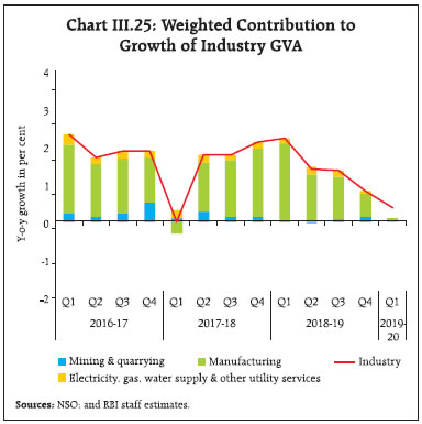
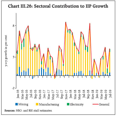
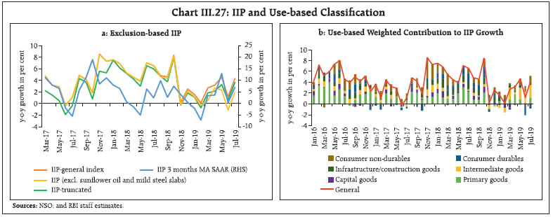 Electricity generation accelerated in Q1:2019-20 due to increased summer demand following the delayed onset of the monsoon. With the seasonal pressure abating, electricity generation from various sources was lower in July and August on a y-o-y basis (Charts III.28). The deceleration in manufacturing GVA in Q1:2019-20 was also reflected in sales growth of manufacturing companies, pulled down mainly by lower sales of automobiles, petroleum, and iron and steel (Chart III.29). The slowdown in sales also mirrored in a sharp decline in profit before tax (Chart III.30). A silver lining was witnessed in the sales of cement, pharmaceuticals and chemical companies, which continued to grow in Q1:2019-20. Overall business sentiment in the Indian manufacturing sector has deteriorated recently. The business assessment index (BAI) fell to 92.5 in Q2:2019-20 (from 108.4 in Q1:2019-20) in the 87th round of the Reserve Bank’s Industrial Outlook Survey (IOS) due to a decline in new orders, contraction in production, lower capacity utilisation and fall in profit margins of the surveyed firms. Business expectations index (BEI) also moderated to 102.2 in Q3:2019-20 (from 112.8 in Q2:2019-20). The manufacturing purchasing managers’ index (PMI) for September 2019 was unchanged at its previous month level, while new orders and employment improved, albeit, marginally, new export orders declined.
III.2.3 Services In Q1:2019-20, services sector growth was the lowest in the last seven quarters, pulled down by financial, real estate and professional services, and construction activity. PADO grew at a healthy rate in Q1:2019-20 and cushioned the loss of pace of GVA from overall services. ‘Trade, hotels, transport, communication and services related to broadcasting’ maintained momentum, though transport services indicators have weakened significantly in the recent period. The sales of commercial vehicles, passenger vehicles, and two-wheelers contracted sharply in July-August. Growth in domestic air passenger traffic accelerated in August. While rail freight traffic contracted in July, domestic air cargo traffic growth improved in August (Chart III.31a and b). The services PMI, however, expanded in July and August, reversing the contraction in June. Of the two key indicators of construction activity, the production of cement accelerated sharply in July before contracting in August, while finished steel consumption moderated in July-August (Chart III.32). Softer domestic steel prices are likely to strengthen steel consumption, going forward. PADO growth moderated sequentially in Q1:2019- 20, reflecting subdued revenue expenditure (net of interest payments and subsidies) of the union and the state governments ahead of elections. The growth of ‘financial, real estate and professional services’ decelerated in Q1:2019-20 mainly due to the poor performance by listed real estate companies notwithstanding a healthy growth in financial services (Chart III.33). In the residential real estate sector, both sales and new launches contracted in Q1:2019-20, indicating sluggish demand (Chart III.34a). With sales outpacing new launches, the inventory overhang has declined somewhat, though the large inventory overhang still has a moderating influence on residential house prices (Chart III.34b).
III.3. Output Gap A detailed analysis of aggregate demand and aggregate supply in the above sections provides an assessment of the state of the economy in H1:2019-20. The output gap – measured by the deviation of actual output from its potential level and expressed as a ratio of potential output – provides a summary measure of demand-supply conditions in the economy. Since potential output and the output gap are both unobservable and their estimates can be sensitive to the choice of methodology and data availability, a pragmatic approach has been followed by applying several methods to estimate potential output. The methods followed are univariate filters such as the Hodrick-Prescott (HP) filter, the Baxter-King (BK) filter and the Christiano-Fitzgerald (CF) filter on the one hand, and multivariate Kalman filter (MVKF) taking into account inflation developments, on the other, to draw robust inferences on the state of the business cycle (Chart III.35). The composite estimate arrived by combining all these measures suggests that the output gap has turned more negative. III.4. Conclusion A combination of domestic and global headwinds has depressed economic activity, especially in terms of aggregate demand. The near-term outlook of the Indian economy is fraught with several risks. First, private consumption, which all along supported economic activity, is now beginning to slow down due to a host of factors. In this context, the performance of large employment generating sectors such as automobile and real estate remains less than satisfactory. Recent measures initiated such as the sharp cut in corporate tax rates, stressed assets funds for the housing sector, infrastructure investment funds, implementation of a fully electronic GST refund system and funds for export guarantee would be helpful. Second, bank credit growth has slowed down and overall fund flows to the commercial sector have declined, partly due to risk aversion and partly due to a slowdown in demand. The recent recapitalisation of public sector banks augurs well for improving credit flows, which are important for reviving private investment activity. Meanwhile, global uncertainties have weakened investment activity at home. Further escalation of trade tensions could adversely impact export prospects, besides delaying the investment upturn. The private corporate sector has not been adding new capacities even as existing capacity utilisation has risen close to its longterm average for several quarters. The recent measures should help kickstart the capex cycle so that new capacities can come on stream and lead to the strengthening of domestic demand in the short-term while boosting the medium-term growth potential of the economy. 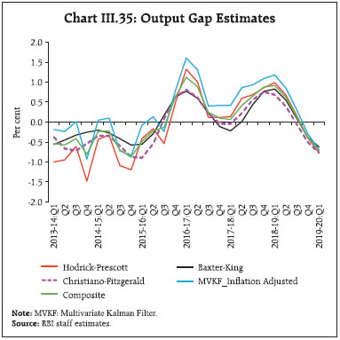
IV. Financial Markets and Liquidity Conditions Domestic financial market segments reacted to evolving domestic and global developments in a diverse manner in the first half of 2019-20. While money markets experienced swift and complete transmission of policy impulses, the government securities and foreign exchange market segments were impacted by domestic economic slowdown and global spillovers. The stock market intermittently scaled new highs amidst sell-off pressures from geo-political tensions. In the credit market, bank lending decelerated reflecting weak demand and risk aversion. Global financial markets were on edge through the first half of 2019-20 (H1:2019-20) amidst sporadic bouts of turbulence around trade tensions, geo-political flashpoints, uncertainty surrounding a chaotic Brexit and a subdued global growth outlook, despite dovish monetary policy stances of leading central banks. Equity markets, in particular, experienced high volatility with stocks of emerging market economies (EMEs) undergoing sell-offs on fears of political unrest in Hong Kong and debt default concerns in Argentina. In bond markets, corporate credit spreads widened as global growth prospects dimmed; on the other hand, ebbing risk appetite coupled with accommodative monetary policy stances resulted in softening of sovereign yields across AEs and EMEs. In the currency market, the US dollar continued to appreciate against other major currencies, reflecting relatively stronger US macroeconomic fundamentals. EME currencies depreciated amidst mounting spillover risks arising from trade tensions and market turmoil. IV.1 Domestic Financial Markets Various segments of the domestic financial market exhibited divergent movements in response to evolving domestic and global developments in H1:2019-20. While money markets witnessed swift and complete transmission, the moderation of yields in bond markets was interrupted by domestic and international factors in August. Equity markets made handsome gains in Q1, with the election related uncertainty coming to an end, but suffered losses on geo-political developments, poor corporate performance and weakness in macroeconomic indicators in Q2. Rising global uncertainty amidst geo-political tensions and domestic cyclical downturn in the economy adversely impacted the foreign exchange market. Overall flow of financial resources to the commercial sector moderated mainly due to reduced credit offtake from banks reflecting weak demand and risk aversion. IV.1.1 Money Market During H1:2019-20, various segments of the money market were impacted by the RBI’s monetary policy actions, stance and liquidity conditions. In the overnight money market, the weighted average call rate (WACR) generally remained below the policy repo rate during H1:2019-20, trading with a downward bias (see Section IV.3 for details). The spread between the WACR and the policy repo rate widened from June, and averaged 6 bps in September. Other overnight money market rates in the collateralised segment, i.e., the tri-party repo rate and the market repo rate, moved largely in tandem with the WACR. Both the tri-party repo rate and the market repo rate remained below the WACR by 7 bps during H1:2019-20 on an average. Volumes in the inter-bank money market shifted from the uncollateralised to the collateralised segment during H1:2019-20. The progressive easing of liquidity conditions led to a fall in the share of call money in total overnight money market volume. Concomitantly, the share of tri-party repo and market repo in total money market volumes increased(Chart IV.1).1 In terms of market microstructure, mutual funds (MFs) continued to be the major lenders in the tri-party repo and market repo segments, with average shares of 59 per cent and 39 per cent, respectively, in H1:2019-20. The major borrowers were public sector banks in the tri-party repo segment and primary dealers (PDs) in the market repo segment. Given deficit liquidity conditions in April and May, lending by MFs declined while borrowing by MFs increased in the collateralised segment during these two months. With systemic liquidity turning surplus since June, lending by MFs increased while borrowing declined marginally in the collateralised segment during June- September. Interest rates on longer-term money market instruments such as certificates of deposit (CDs), commercial papers (CPs) and Treasury Bills (T-bills) of 3-month maturity responded in varying degrees to policy rate cuts and the shift in the policy stance from neutral to accommodative during H1:2019- 20 (Chart IV.2). Interest rates on CPs moderated noticeably during H1, particularly those issued by non-banking financial companies (NBFCs), although CP rates traded above CD rates. In comparison, yields on 3-month T-bills moderated by a greater extent during the period. 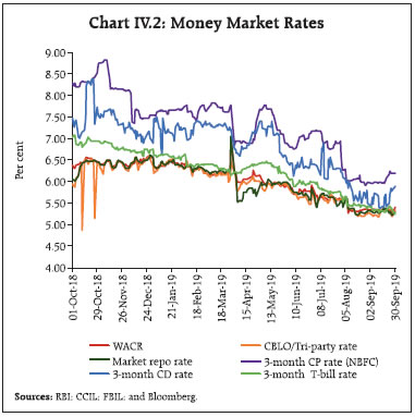 In the wake of easy liquidity conditions in the banking system, fresh issuances of CDs declined to ₹1,75,305 crore during H1:2019-20 (up to September 13, 2019) as compared with ₹1,98,829 crore during the corresponding period of 2018-19. Primary issuances of CPs also declined to ₹11,92,277 crore during H1:2019-20 from ₹13,58,117 crore during H1:2018- 19, with more than 99 per cent of the issuances by companies with A1+ rating. CP issuances moderated from July reflecting heightened risk aversion in view of downgrading of a few CP issuers in June and July 2019. Nevertheless, interest rates in the primary CP market – as reflected in the weighted average discount rate (WADR) – moderated sharply by 130 bps during H1:2019-20, facilitated by the easing of liquidity conditions (Chart IV.3a). During this period, non-financial corporates and NBFCs were the major issuers in the CP market (Chart IV.3b). 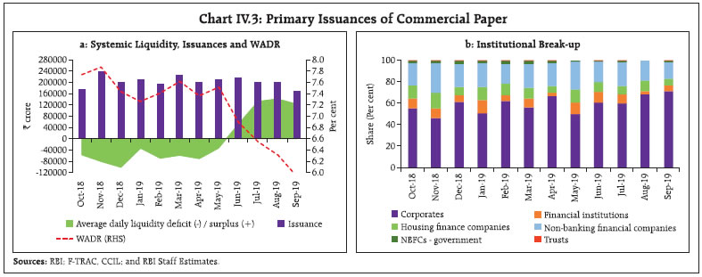 Risk premium in the money market (i.e., spread between 3-month CPs and 3-month T-bills) remained high at an average of 99 bps during April-July reflecting the downgrading of some CP issuers in June-July and tight liquidity conditions during April-May (Chart IV.4a). The risk premium declined sharply to an average of 64 bps in August-September on account of (i) the liquidity effect emanating from the switch in liquidity conditions from deficit to surplus since the beginning of June 2019; (ii) the predominance of issuances by top rated issuers raising funds at competitive rates; and (iii) the measures taken by the government and the Reserve Bank to provide liquiditysupport to NBFCs.2 The spread between 3-month CP rate of NBFCs and non-NBFCs narrowed (average of 23 bps in H1:2019-20 vis-à-vis 44 bps in H2:2018-19), notwithstanding some intermittent spikes (Chart IV.4b). 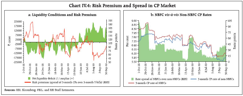
| Table IV.1: Policy Transmission in the Money Market | | (Basis points) | | H1: 2019-20 | Change in Rates | | Repo | WACR | Tri-party Repo | Market Repo | 3-month CD | 91-day T-bill | 3-month CP (NBFCs) | | April 3 to June 4 | -25 | -32 | -43 | -37 | -33 | -16 | -5 | | June 6 to August 6 | -25 | -24 | -18 | -25 | -48 | -44 | -80 | | August 7 to September 30 | -35 | -23 | -28 | -32 | -6 | -38 | 20 | | Cumulative (April 3 - September 30) | -85 | -79 | -89 | -94 | -87 | -98 | -65 | | Sources: RBI; CCIL; FBIL; and Bloomberg. | During H1:2019-20, policy transmission was nearly complete in all segments of the money market. Of the three policy announcements during this period, the maximum impact was felt after the June policy – which signaled both a rate cut and a change in the stance from neutral to accommodative – particularly at the longer end of the money market spectrum (Table IV.1). Thus, both the announcement effect of repo rate cuts and the liquidity effect of surplus conditions were instrumental in securing policy transmission. IV.1.2 Government Securities (G-Sec) Market G-sec yields traded with a softening bias at the beginning of Q1:2019-20, taking cues from several positive developments during Q4:2018-19, viz., monetary policy easing and a change in the policy stance from calibrated tightening to neutral; injection of durable liquidity; announcement of the voluntary retention route (VRR); and successive benign inflation prints. The softening of yields was, however, ephemeral and they started hardening in April 2019, partly due to (i) no change in the policy stance contrary to market expectation; (ii) sustained higher crude oil prices after the US announced stopping of imports from Iran and supply disruptions in Libya and Venezuela; and (iii) depreciation of the Indian rupee (INR). Consequently, the benchmark yield hardened by 6 bps during April 2019 despite injection of durable liquidity through a US dollar buy/ sell swap. Amidst heightened trade tensions, yields softened by 38 bps by during May in the wake of election results indicating political stability. This was aided by infusion of liquidity through open market operation (OMO) purchases and lower crude oil prices. The softening trend continued in June with the benchmark yield declining further by 15 bps during the month, as market sentiment was buoyed by a further reduction in the policy rate, a shift in the policy stance and continued OMO purchases by the RBI. The moderation in yields extended into Q2 even as the market sentiment was unsettled by fears of excess supply of paper. In fact, G-Sec yields remained volatile through July 2019. Nonetheless, positive Budget announcements such as pegging of the fiscal deficit at 3.3 per cent of GDP and unchanged quantum of borrowing vis-à-vis the Interim Budget bolstered market sentiment. This was also reflected in renewed buying by foreign portfolio investors (FPIs) in the debt market. Moreover, benign inflation prints triggered market expectations of further rate cuts. All these factors resulted in the benchmark yield softening further by 50 bps during July, touching a low of 6.33 per cent on July 16, 2019 – its lowest level during H1:2019-20. Despite positive developments such as a larger than expected rate cut of 35 bps by the MPC, rollback of surcharge on FPIs, higher than expected surplus transfer by the RBI, the G-sec market remained wary in August on concerns over fiscal slippage arising from anticipation of a stimulus, and domestic/geo-political tensions. Accordingly, the benchmark yield hardened by 19 bps during August 2019, paring previous gains (Chart IV.5). 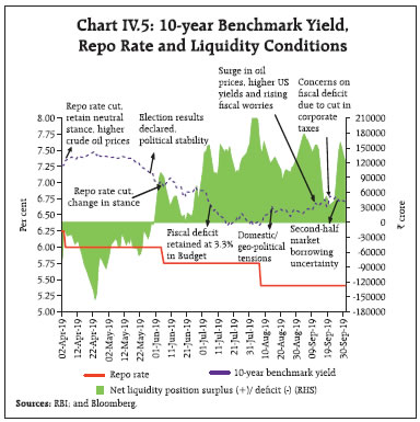 The hardening bias of benchmark yield continued in September owing to (i) rising crude oil prices following the attack on Saudi oil refineries; (ii) lingering fiscal concerns; and (iii) surge in overnight indexed swap (OIS) rates fuelled by a rise in US bond yields. Subsequent reassurances by the Saudi authorities on restoring normalcy assuaged market apprehensions somewhat and softened crude prices thereafter. Moreover, large buying support from state owned banks, market expectation of a further rate cut and easing of limit on foreign investment in gilts softened yields towards the end of September. Overall, the benchmark yield softened by 65 bps during H1:2019-20, closing at 6.70 per cent on September 30, 2019. The yield curve, which underwent shifts in H1:2019-20, is characterised by its level and slope(Chart IV.6a).3 Since the April monetary policy announcement, the average level of yield has softened by 50 bps, driven down by: (i) cumulative policy easing by 85 bps, accompanied by a change in the monetary policy stance; (ii) build-up of surplus liquidity position aided by liquidity infusion through OMOs and forex buy/sell swaps; (iii) ongoing liquidity support measures to NBFCs; and (iv) benign domestic inflation prints. Since the August policy announcement (up to September 30, 2019), however, the average level has firmed up by 24 bps even as the yield curve has become steeper, reflecting inter alia fears of a large shortfall in government revenue after the announcement of corporate tax rate cuts by the Government, apprehensions of crude oil supply disruption and heightened geo-political uncertainties/ financial market turmoil in some EMEs (Chart IV.6b). 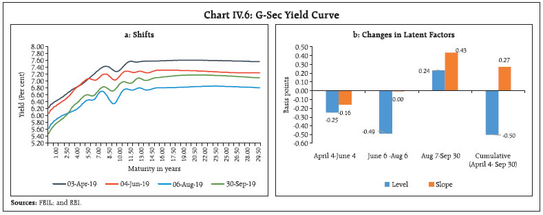 The introduction of the VRR and increased investment limits for G-Sec boosted overseas investor interest in debt instruments at the beginning of 2019-20. With benign inflation prints, coupled with political stability arousing investors’ appetite, FPIs remained net buyers in the G-Sec market during H1:2019-20, although they turned net sellers in September due to geo-political tensions and tepid domestic economic outlook (Chart IV.7). At the short end of the primary segment, T-bill yields softened during H1:2019-20 tracking the benchmark yield (Chart IV.8). At the longer end, issuances of state development loans (SDLs) were moderate during H1:2019-20 as against the front-loading of issuances by the GoI. The weighted average cumulative spread of SDLs’ cut-offs over the corresponding tenor G-sec at 52 bps in H1:2019-20 (as on September 30) was comparable to 54 bps in H1:2018-19 (Chart IV.9). During H1:2019-20, the average inter-state spread on securities of 10-year tenor at 4 bps remained identical to that recorded in H1:2018-19. IV.1.3 Corporate Bond Market Corporate bond yields eased sharply during H1:2019- 20, largely tracking G-sec yields and reflecting transmission of policy repo rate cuts (Chart IV.10a). During this period, 5-year AAA corporate bond yields softened by 66 basis points – from 8.10 per cent at end-March 2019 to 7.44 per cent at end- September 2019 – in response to the cumulative policy rate reduction of 85 basis points (excluding the reduction in February 2019 during the current easing cycle). Moreover, easy liquidity conditions also led to a reduction in the risk premia. Illustratively, the yield spread (5-year AAA corporate bonds over 5-year G-sec) on bonds issued by public sector undertakings (PSUs), financial institutions (FIs) and banks, NBFCs, and corporates declined by 32 bps, 20 bps and 19 bps points, respectively, during this period. State Bank of India (SBI) and ICICI Bank 5-year credit default swap (CDS) spreads – which indicate credit default risk – also declined by 23 bps and 21 bps, respectively. 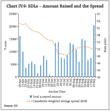 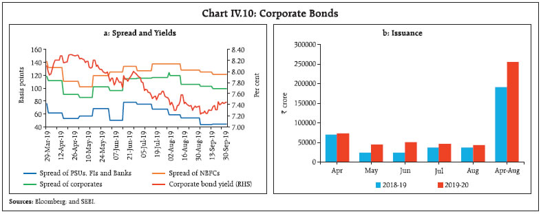 Resource mobilisation through issuances of corporate bonds in the primary market increased sharply by 34.4 per cent to ₹2.6 lakh crore during April-August 2019 from ₹1.9 lakh crore a year ago (Chart IV.10b). Almost the entire resource mobilisation in the corporate bond market (97.3 per cent) continued to be through the private placement route. Investments by FPIs in corporate bonds declined to ₹2.03 lakh crore at end- September 2019 from ₹2.19 lakh crore at end-March 2019. Consequently, FPIs’ utilisation of the approved limit for investment in corporate bonds came down to 64.0 per cent at end-September 2019 from 75.9 per cent at end-March 2019. The average daily turnover in the corporate bond market increased to ₹8,261 crore during H1:2019-20 (up to September 27, 2019) from ₹7,131 crore during H1:2018-19. IV.1.4 Equity Market Equity markets scaled records in the immediate aftermath of the 2019 general elections. Thereafter, they corrected during Q2:2019-20 due to a combination of domestic and global factors which dampened market sentiment, closing at about the same level as at the beginning of the year (Chart IV.11a). The BSE Sensex registered modest gains in April 2019, aided by continued FPI inflows, the policy repo rate cut by the RBI and positive global cues, notwithstanding weak corporate earnings results. Markets witnessed a sharp downturn during early May 2019 as trade tensions between the US and China intensified. Investor sentiment, however, turned positive later in the month buoyed by the prospects of a stable government and expectations of further monetary easing by the RBI. Market exuberance pushed the BSE Sensex to a record high of 40268 on June 3, 2019 but this rally proved transient as sentiment turned bearish after a default by a housing finance company triggered liquidity concerns in the NBFC sector. The downtrend deepened in July over some Budget proposals such as (i) tax on super rich; (ii) buyback tax; and (iii) increase in minimum public shareholding in listed companies. Negative cues from global equity markets, reporting of a borrowing fraud in a public sector bank, concerns over lackluster corporate earnings results for Q1: 2019-20, slow progress of the monsoon and continued FPI outflows due to the proposed increase in tax surcharge for FPIs registered as non-corporates exacerbated the decline in July 2019. 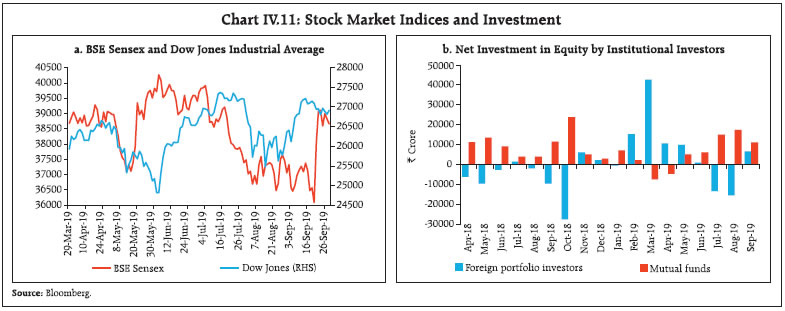 The equity market declined marginally in August 2019. Adverse domestic developments such as tepid corporate earnings results for Q1: 2019-20, lukewarm industrial activity and auto sales, and negative global cues, viz., political unrest in Hong Kong, debt default in Argentina and uncertainty over the US-China trade negotiations completely nullified the positive impact of government measures like rollback of the super-rich tax on FPIs, frontloading of capitalisation of public sector banks and deferment of a hike in registration fees for automobiles. The BSE Sensex surged nearly 5 per cent on September 20 spurred by the reduction in the corporate tax rate – the biggest rally in over a decade. Subsequently, the BSE Sensex corrected on concerns about the health of the domestic banking sector and political uncertainty in the US. Overall, the BSE Sensex registered a gain of 3.6 per cent during September 2019. While FPIs were net sellers to the tune of ₹605 crore in the equity market, domestic institutional investors, particularly MFs, made heavy purchases amounting to ₹50,316 crore during H1: 2019-20 (Chart IV.11b). In the primary segment of the equity market, resource mobilisation through public and rights issues grew nearly five times to ₹59,618 crore during April- August 2019 as compared with ₹12,028 crore in the corresponding period of the previous year. IV.1.5 Foreign Exchange Market Since April 2019, the INR traded with a depreciating bias, dipping to a low of ₹72.19 per US dollar (reference rate) on September 3, 2019. The fall in the INR was in line with many EME currencies experiencing depreciation vis-à-vis the US dollar, which was pronounced in August and September. Overall, the fall in the INR during April-September 2019 was due to equity sell-offs by FPIs and strengthening of the US dollar, triggered by rising risk aversion among investors on escalating US-China trade tensions and concerns over tepid global growth. While the INR depreciated by 2.1 per cent vis-à-vis the US dollar on September 30, 2019 over end-March 2019, it was modest in comparison with the depreciation of many of its EME peers such as the Malaysian ringgit, the South African rand, the Chinese yuan and the Brazilian real (Chart IV.12a). 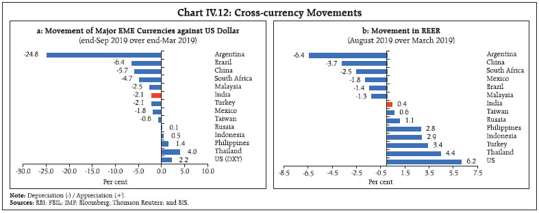 In terms of the 36- and 6-currency nominal effective exchange rate (NEER), the INR appreciated by 0.4 per cent and 1.1 per cent, respectively, at end-September, 2019 over March (average) 2019. Similarly, the INR, in terms of both 36- and 6-currency real effective exchange rate (REER), appreciated during the same period (Table IV.2). The appreciation in REER of the INR between March and August 2019 was modest as compared with that of the Taiwan dollar, the Russian ruble, the Philippine peso, the Indonesian rupiah, the Turkish lira, and the Thai baht (Chart IV.12b). | Table IV.2: Nominal and Real Effective Exchange Rates – Trade-based Weights | | (Base: 2004-05 = 100) | | Item | Index: End- September 2019 (P) | Appreciation (+) / Depreciation (-) (Per cent) | | End- September 2019 over March 2019 | March 2019 over March 2018 | | 36-currency REER | 116.7 | 1.3 | -1.2 | | 36-currency NEER | 73.9 | 0.4 | -1.7 | | 6-currency REER | 126.6 | 2,7 | -0.9 | | 6-currency NEER | 64.6 | 1.1 | -1.9 | | ₹/US$ | 70.69 | -1.7 | -6.4 | P: Provisional.
Sources: RBI; and FBIL. | IV.1.6 Credit Market In the credit market, offtake during the year (up to mid-September) has been muted; both, low momentum and unfavourable base effects dragged down non-food credit growth (Chart IV.13). The seasonal decline in credit during Q1:2019-20 was more pronounced than in the corresponding quarter of the previous year. The offtake during Q2 (up to mid-September) has been subdued as compared with the corresponding quarter of the previous two years. The slowdown in credit growth was led by public sector banks and private sector banks, while credit growth of foreign banks continued to be modest, despite some uptick in the recent period (Chart IV.14). While credit growth to agriculture and personal loans remained broadly unchanged in the last one year, credit growth to industry moderated in the last four months after accelerating continuously between August 2018 and April 2019. Credit growth to services has decelerated sharply since January 2019 (Chart IV.15a). Of the incremental non-food credit flow during the year (August 2019 over August 2018), personal loans accounted for the largest share, followed by services and industry (Chart IV.15b). Within personal loans, credit offtake has been broadly concentrated in two segments, viz., housing and credit card outstanding. Within industry, credit growth to beverages and tobacco, cement, engineering, vehicles, construction and infrastructure (viz., power, telecommunications and roads) accelerated. Credit quality has deteriorated with both the stressed assets ratio and the non-performing assets (NPA) ratio increasing marginally in June 2019 after four successive quarters of decline (Chart IV.16a). Sector-wise analysis indicates that the NPA ratio deteriorated for all sectors in June 2019, barring industry (Chart IV.16b). Banks have reduced their investment in the non-statutory liquidity ratio (SLR) portfolio by about ₹35,000 crore in 2019-20 (up to September 13). This is notwithstanding a marginal increase in exposure to CPs in contrast to a decline in H2:2018-19. With both non-SLR investment and non-food credit undergoinga decline, adjusted non-food credit4 growth decelerated during the year so far (Chart IV.17). With muted credit offtake and decline in non- SLR investments, banks have augmented their SLR portfolios despite the reduction in SLR by RBI. Banks held excess SLR of 6.9 per cent of net demand and time liabilities (NDTL) on August 30, 2019 as compared with 6.3 per cent of NDTL at end-March 2019 (Chart IV.18). Overall, financial flows to the commercial sector in 2019-20 so far (up to mid-September) have been lower than in the same period last year due to a decline in funding from banks and lower funding from non-bank sources. Among domestic non-bank sources of funding, public issues of equity and private placement increased significantly. Among foreign sources, both external commercial borrowings and foreign direct investment (FDI) registered sharp increases (Table IV.3). Notably, a new framework for external commercial borrowings was announced in January 2019 to improve the ease of doing business; subsequently, end-use provisions were also rationalised in July 2019. 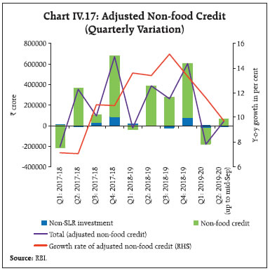 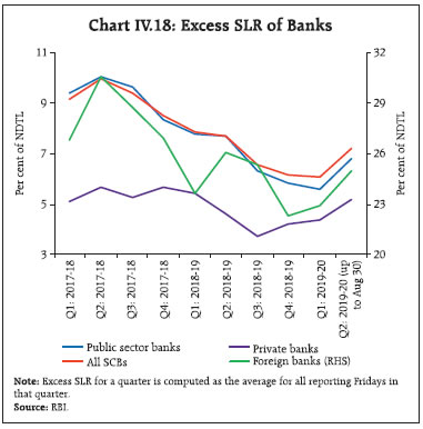
| Table IV.3: Flow of Funds to the Commercial Sector | | (Amount in ₹ crore) | | Item | April to mid-Sep | | 2018-19 | 2019-20 | | Amount | Per cent to Total | Amount | Per cent to Total | | A. Flow from banks, i.e., Adjusted non-food credit (A1+A2) | 1,85,083 | 25.1 | -1,28,760 | -141.5 | | A1. Non-food credit | 1,65,187 | 22.4 | -93,688 | -103.0 | | A2. Non-SLR investment by scheduled commercial banks | 19,896 | 2.7 | -35,072 | -38.5 | | B. Flow from non-banks (B1+B2) | 5,51,004 | 74.9 | 2,19,755 | 241.5 | | B1. Domestic sources | 4,44,696 | 60.4 | 13,562 | 14.9 | | 1. Public issues by non-financial entities * | 6,253 | 0.8 | 58,326 | 64.1 | | 2. Gross private placement by non-financial entities * | 47,379 | 6.4 | 62,495 | 68.7 | | 3. Net issuance of CPs subscribed by non-banks | 2,53,669 | 34.5 | 19,118 | 21.0 | | 4. Net credit by housing finance companies $ | 52,181 | 7.1 | -6,003 | -6.6 | | 5. Total accommodation by 4 RBI regulated AIFIs * | 40,032 | 5.4 | -4,774 | -5.2 | | 6. NBFCs-ND-SI and deposit taking NBFCs (net of bank credit) $ | 41,200 | 5.6 | -1,25,600 | -138.0 | | 7. LIC’s net investment in corporate debt, infrastructure and social sector^ | 3,982 | 0.5 | 10,000 | 11.0 | | B2. Foreign sources | 1,06,308 | 14.4 | 2,06,193 | 226.6 | | 1. External commercial borrowings / FCCB * | -653 | -0.1 | 54,073 | 59.4 | | 2. Foreign direct investment to India ^ | 1,06,961 | 14.5 | 1,52,119 | 167.2 | | C. Total flow from banks and non-banks (A+B) | 7,36,087 | 100.0 | 90,995 | 100.0 | $: Up to Jun ^: Up to Jul *: Up to Aug.
Sources: RBI; SEBI; BSE; NSE; NHB; LIC and merchant banks. | IV.2 Monetary Policy Transmission The response of deposit and lending rates of commercial banks to the cumulative reduction in the policy repo rate by 110 bps during the easing cycle of monetary policy starting from February 2019 has been muted so far (Table IV.4). While the weighted average lending rate (WALR) on fresh rupee loans decreased by only 29 bps (February-August 2019), the WALR on outstanding rupee loans, in contrast, increased by 7 bps over the same period. The inadequate transmission essentially reflects slow adjustment in bank term deposit rates. This, in turn, reflects the long maturity profile of bank deposits at fixed interest rates. | Table IV.4: Transmission to Deposit and Lending Rates | | (Basis points) | | Period | Repo Rate | Term Deposit Rates | Lending Rates | | Median Term Deposit Rate | WADTDR | 1-year Median MCLR | WALR - Outstanding Rupee Loans | WALR - Fresh Rupee Loans | | Feb-Mar 2019 | -25 | -1 | -2 | -5 | -3 | -24 | | Apr-May 2019 | -25 | -6 | 0 | 0 | 7 | 13 | | Jun-Jul 2019 | -25 | -4 | -4 | -15 | 2 | -9 | | Aug-Sep 2019* | -35 | -15 | 2 | -15 | 1 | -9 | | Feb-Sep 2019* | -110 | -26 | -4 | -35 | 7 | -29 | *: Latest data on WALR and WADTDR pertains to August 2019.
WADTDR: Weighted Average Domestic Term Deposit Rate. WALR: Weighted Average Lending Rate.
MCLR: Marginal Cost of Funds based Lending Rate.
Source: RBI. |
The WALR on fresh rupee loans declined during February-August 2019 across bank groups, with the largest decline observed in foreign banks and the least in public sector banks (Chart IV.19). As the lending activity of public sector banks was constrained by higher NPAs and lower capital adequacy vis-à-vis private sector banks, the share of fresh rupee loans of private sector banks overtook that of PSBs in August 2019 (Chart IV.20). Actual lending rates comprise marginal cost of funds based lending rate (MCLR) and a spread. Banks charged the lowest spread (WALR on outstanding rupee loans over 1-year MCLR) on housing loans during August 2019 reflecting (i) lower probability of default; (ii) availability of good collateral; and (iii) competition from NBFCs (Chart IV.21). At the other end of the spectrum, the spread charged on ‘other personal loans’ was the highest. The spread between MCLR/WALR on fresh rupee loans/outstanding rupee loans and G-sec yields has risen sharply through 2019, reflecting complete transmission of policy rate to bond markets as against muted transmission to credit markets (Chart IV.22). 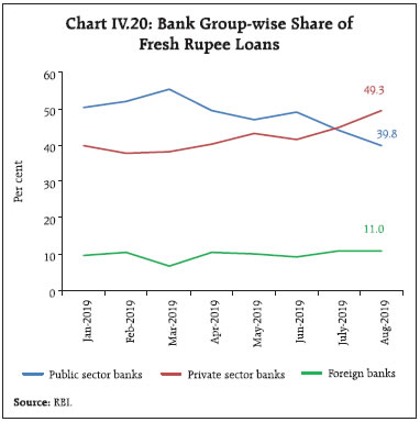 One of the important factors impeding monetary transmission is administered interest rates on small saving schemes set by the Government of India. These administered interest rates are linked to market interest rates on G-secs with a lag and are fixed on a quarterly basis at a spread ranging from 0-100 bps over and above G-sec rate of comparable maturities. Interest rates on small saving schemes were revised on June 28, 2019 for Q2: 2019-20, which came into effect from July 1, 2019 whereby the rates of interest on all small savings schemes (except savings deposit) were reduced by 10 bps. Even after the reduction, however, the small saving rates of various schemes continued to be higher by 18-62 bps in Q2:2019-20 than the formula-based interest rates. With the Government deciding to keep the interest rates on small savings unchanged for Q3:2019-20 notwithstanding a decline in G-sec yields in the reference period (June-August 2019), the wedge between the current small saving rates on various schemes and the formula-based rates for Q3:2019-20 has widened further to 70-110 bps (Table IV.5). 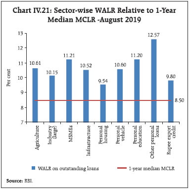 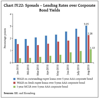 The MCLR system of pricing loans lacks transparency as it is internal to each bank and borrowers have no way of ascertaining as to how it has been arrived at. While it may not matter for new borrowers as they are able to compare overall lending rates across banks and take a decision in their best interest, it impacts existing borrowers as they cannot easily ascertain the factors that lead to the changes in MCLR. The MCLR system also did not deliver effective transmission as banks were slow to adjust their deposit interest rates which, in turn, had a bearing on their lending rates. | Table IV.5: Interest Rates on Small Savings Instruments – Q3:2019-20 | | Small Savings Scheme | Maturity (Years) | Spread (Percentage point)$ | Average G-sec Yield (Per cent) of Corresponding Maturity (June 2019 to August 2019) | Formula-based Rate of Interest (Per cent) (applicable for October to December 2019) | Government Announced Rate of Interest (Per cent) in Q3 | Difference (Basis points) | | (1) | (2) | (3) | (4) | (5) = (3) + (4) | (6) | (7) = (6)-(5) | | Savings Deposit | - | | | | 4.00 | - | | Public Provident Fund | 15 | 0.25 | 6.81 | 7.06 | 7.90 | 84 | | Time Deposits | | | | | | | | 1 Year | 1 | 0 | 5.85 | 5.85 | 6.90 | 105 | | 2 Year | 2 | 0 | 6.01 | 6.01 | 6.90 | 89 | | 3 Year | 3 | 0 | 6.18 | 6.18 | 6.90 | 72 | | 5 Year | 5 | 0.25 | 6.50 | 6.75 | 7.70 | 95 | | Post Office Recurring Deposit Account | 5 | 0 | 6.50 | 6.50 | 7.20 | 70 | | Post Office Monthly Income Scheme | 5 | 0.25 | 6.47 | 6.72 | 7.60 | 88 | | Kisan Vikas Patra | 113 Months | 0 | 6.81 | 6.81 | 7.60 | 79 | | NSC VIII issue | 5 | 0.25 | 6.66 | 6.91 | 7.90 | 99 | | Senior Citizens Savings Scheme | 5 | 1.00 | 6.50 | 7.50 | 8.60 | 110 | | Sukanya Samriddhi Account Scheme | 21 | 0.75 | 6.81 | 7.56 | 8.40 | 84 | $: Spreads for fixing small saving rates as per Government of India Press Release of February 16, 2016.
Note: Compounding frequency varies across instruments.
Sources: Government of India; and RBI staff estimates. | To address these concerns, the Reserve Bank, in pursuance of the recommendations of an Internal Study Group (Chairman: Dr. Janak Raj), mandated that all scheduled commercial banks (excluding regional rural banks) should link all new floating rate personal or retail loans and floating rate loans to Micro and Small Enterprises (MSEs) to the policy repo rate or 3-month T-bill rate or 6-month T-bill rate or any other benchmark market interest rate published by Financial Benchmarks India Private Ltd. (FBIL), effective October 1, 2019. Banks are free to choose the spread over the benchmark rate, subject to the condition that the credit risk premium may undergo change only when the borrower’s credit assessment undergoes a substantial change, as agreed upon in the loan contract. External benchmarks are transparent as they are available in the public domain and hence easily accessible to the borrowers. The external benchmark framework will improve transmission as (i) the lending rates will be referenced to one of the prescribed benchmark rates for new borrowers; and (ii) banks would need to reset the benchmark rate at least once in three months for existing borrowers. IV.3 Liquidity Conditions and the Operating Procedure of Monetary Policy The RBI Act 1934 amended in 2016 requires the RBI to place the operating procedure relating to the implementation of monetary policy and changes thereto from time to time, if any, in the public domain. During H1:2019-20, liquidity management operations by the RBI were conducted within the broad framework discussed in the Monetary Policy Reports of October 2018 and April 2019. In addition to regular operations during H1:2019-20, the RBI resorted to fine-tuning variable rate repo and reverse repo auctions. Liquidity amounting to ₹5,09,585 crore was injected through the regular 14-day repos, while liquidity amounting to ₹93,39,315 crore was absorbed through reverse repos of maturity ranging from overnight to 63 days. In addition, liquidity aggregating ₹47,128 crore was injected through variable rate repos of maturity ranging from 1 to 3 days. Four open market operation (OMO) purchase auctions and one US$ 5 billion buy/sell swap auction was conducted by the RBI during H1:2019-20. Furthermore, the SLR was cumulatively reduced by 50 bps during H1 – 25 bps each effective April 13 and July 6, respectively, – to 18.75 per cent of NDTL of banks, in accordance with the roadmap announced in December 2018 with a view to enabling banks to raise structural liquidity. Drivers and Management of Liquidity RBI’s forex operations including US$ 5 billion buy/ sell swap auction and net OMO purchases were the major drivers augmenting liquidity in H1:2019-20, which was absorbed through operations under the liquidity adjustment facility (LAF) by the RBI. This contrasts with H2:2018-19 when a large expansion in currency in circulation (CiC) resulted in a leakage of liquidity from the banking system, which had to be replenished through large scale open market purchase operations and liquidity injections under the LAF (Chart IV.23). During H1:2019-20, the increase in CiC at ₹49,378 crore (2.3 per cent) was muted in comparison with the significantly higher increase of ₹95,896 crore (5.2 per cent) in the corresponding period of 2018-19. As a result, growth in CiC (y-o-y) was consistently lower than in the previous year (Chart IV.24). In April and May, liquidity conditions were in deficit due to restrained government spending and high demand for cash. The unwinding of GoI cash balances – a regular feature every year in April – was much lower in the current year due to the imposition of the model code of conduct during elections restricting government spending. Combined with rising currency demand, this caused liquidity tightness. Consequently, the RBI conducted a US$/INR buy/ sell swap auction of US$ 5 billion (₹34,874 crore) for a tenor of 3 years in April and two OMO purchase auctions in May amounting to ₹25,000 crore to inject durable liquidity into the system. It also injected liquidity of ₹51,403 crore on a daily net average basis under the LAF during these two months. The situation changed in June when liquidity conditions turned to surplus due to increased spending after government formation at the Centre, net forex purchases by the RBI and return of currency to the banking system post-elections. The RBI also conducted two OMO purchase auctions amounting to ₹27,500 crore. Consequently, total injection of durable liquidity in Q1:2019-20 – through bothOMOs5 and US$/INR swap auction – amounted to ₹87,414 crore (Chart IV.25). The RBI absorbed surplus liquidity of ₹51,710 crore on a daily net average basis under the LAF in June. 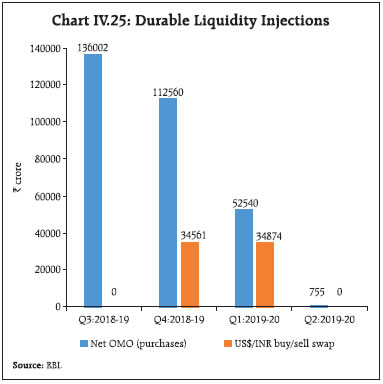 Surplus liquidity conditions persisted in July on account of (i) return of currency to the banking system; and (ii) the Reserve Bank’s net forex purchase operations. Although liquidity continued to be in surplus in August, its drivers were distinctly different. First, currency expansion picked up, draining systemic liquidity. Second, increasing geo-political uncertainties in EMEs from political unrest in Hong Kong and meltdown of financial markets in Argentina resulted in capital outflows necessitating forex market (sales) intervention by the RBI. These pressures were, however, more than offset by a large drawdown of GoI balances, with the Central Government resorting to ways and means advances (WMA) for a major part of the month. In September, the surplus moderated with the build-up of large government cash balances, particularly with the receipt of advance taxes after September 15 (Chart IV.26). Nevertheless, absorption of liquidity on a daily net average basis under the LAF soared to ₹1,31,370 crore during Q2:2019-20 in contrast to a net injection of ₹17,409 crore in Q1. Simultaneously, transient liquidity needs were met through variable rate repos of smaller tenors (1-3 days) in addition to the regular 14-day term repos. 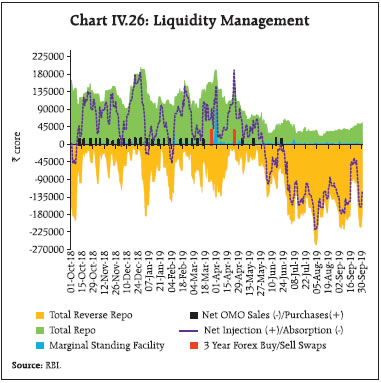 To sum up, the RBI’s forex operations and currency expansion were the prime drivers of durable liquidity in the banking system in H1:2019-20, while government spending was the key driver of frictional liquidity movements. With the Reserve Bank injecting durable liquidity through OMOs and US$/INR buy/sell swap auction, net LAF positions mirrored movements in government cash balances (Chart IV.27). The temporary mismatches between receipts and payments of the government during H1:2019-20 were partly met through recourse to cash management bills (CMBs) on two occasions of maturity ranging 10-33 days aggregating ₹50,000 crore. Fine-tuning operations through variable rate auctions continued to be the key feature of liquidity management during H1:2019-20. Liquidity injections were made through repo auctions of maturities ranging from overnight to 14 days, while reverse repos ranging from overnight to 7 days were frequently used for absorbing liquidity (Table IV.6). | Table IV.6: Fine-tuning Operations through Variable Rate Auctions in H1:2019-20 | | Operation | Repo (maturity in days) | Reverse Repo (maturity in days) | | 1 | 2 | 3 | 14* | 1 | 2 | 3 | 4 | 7 | 14 | 63 | | Frequency (number of times) | 1 | 1 | 1 | 52 | 100 | 5 | 27 | 4 | 33 | 1 | 1 | | Average volume (₹ crore) | 8,825 | 25,003 | 13,300 | 5,09,585 | 65,62,076 | 3,65,300 | 16,88,773 | 2,90,358 | 4,31,458 | 550 | 800 | *: Regular 14-day variable rate repo operations
Source: RBI | Operating Target and Policy Rate During H1, the WACR – the operating target of monetary policy – generally traded below the repo rate during May-September (Chart IV.28). The objective of monetary policy is to keep the WACR aligned to the policy repo rate and contain volatility caused by exogeneous shocks within the interest rate corridor defined by the lower (reverse repo rate) and the upper (marginal standing facility rate) bounds. There are, however, instances when the WACR breached the corridor on account of: (i) uncertainty about liquidity conditions; (ii) market microstructure issues such as quarter-end or year-end liquidity tightness (due to advance tax payments or window dressing of balance sheet); (iii) structural changes in the monetary policy implementation framework (for instance, making the policy corridor non-symmetric by raising the MSF rate 300 bps above the policy repo rate in the aftermath of the taper tantrum episode); and (iv) banks’ expectations of future interest rates. In this context, an empirical exercise identifies the factors contributing to the occurrence of such episodes (Box IV.1). 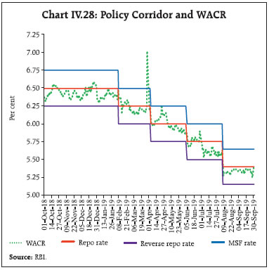
Box IV.1: WACR Breaching the Policy Corridor: Causes and Determinants Determinants of the spread (WACR over the policy repo rate) include market expectations, risk measures, liquidity conditions, and market microstructure variables (Table IV.1.1). Liquidity conditions have been defined as the net LAF position on any day as a proportion of the average daily CRR requirement. An increase (decline) in this ratio would signify tightening (easing) of liquidity conditions leading to an increase (reduction) in the spread under deficit liquidity conditions. Skewed distribution of central bank’s liquidity among banks may impact the WACR spread adversely, i.e., greater heterogeneity in distribution of liquidity (a few participants cornering a large part of central bank liquidity) is likely to increase the demand for funds in the call money market and increase the spread (Linzert and Schmidt, 2008; Kumar et al, 2017). This variable has been approximated by the share of call market transactions in the total overnight market volume. | Table IV.1.1: Description of Variables | | Variable | Measured by | Expected impact6 | | Lagged spread | First lag of spread (where spread is defined as weighted average call money market rate minus repo rate) | increase | | Within period expectation | 14 day Mumbai Inter-Bank Outright Rate (MIBOR) rate minus repo rate | increase | | Liquidity conditions | Net LAF position/ average daily cash reserve requirement | increase | | Interest rate uncertainty | Uncertainty about interest rate at 2 week horizon: GARCH(1,1) conditional volatility of 14 day MIBOR rate | increase | | Liquidity uncertainty | GARCH(1,1) conditional volatility of reserve fulfilment | increase | | Liquidity distribution | Ratio of the volume in call money to total volume in overnight market | increase | | Corridor width dummy | Corridor width as a dummy variable – it takes the value of 1 (if corridor width < 100 bps) or 0 (if corridor width > 100 bps) | increase | | Quarterly dummy | Quarter-end phenomenon – value 1 for quarter-end and 0 otherwise | increase | In addition to the above, two dummies are also used for the empirical exercise keeping in view the idiosyncratic factors witnessed during the sample period. First, a dummy for changes in the liquidity management implementation framework is introduced for the period when the MSF rate was raised by 300 bps above the repo rate, as part of the policy response to domestic financial market turmoil in the aftermath of the taper tantrum. Accordingly, a value of 1 is taken for each day from July 17 to October 28, 2013 representing the post taper tantrum period and 0 otherwise. Second, a value of 1 for the period November 9, 2016 to January 31, 2017 and 0 otherwise is considered for the post-demonetisation period when the return of currency to the banking system resulted in large surplus liquidity with the WACR breaching the lower bound of the corridor, i.e., dropping below the reverse repo rate. Following an empirical strategy used in the literature on regime shifts in capital flows (Forbes and Warnock, 2012), a logistic regression analysis (binary logit model) was undertaken to estimate the probability of the call rate breaching the interest rate corridor (Prabu and Bhattacharyya, 2019). The following logit model was used: 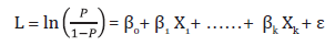
where p indicates the probability of the call money rate breaching the interest rate corridor. L is the logit function and Xs refers to the independent variables. The model is estimated based on daily data from May 2011 to June 2019 covering 1960 observations (Table IV.1.2). The results suggest that an increase in skewness of liquidity distribution will increase the odds of the call rate breaching the interest rate corridor. Similarly, an increase in liquidity conditions (more injection by the RBI relative to the CRR requirement of banks) and an increase in interest rate uncertainty also increases the odds of the call rate lying outside the interest rate corridor. | Table IV.1.2: Logit Model – Results | | Variables | Odds Ratio | | 1 | 2 | | Lagged spread | 1.002 | | | (0.587) | | Within period expectation | 1.001* | | | (0.093) | | Liquidity uncertainty | 1.01 | | | (0.856) | | Liquidity distribution | 1.05*** | | | (0.000) | | Interest rate uncertainty | 1.01*** | | | (0.005) | | Liquidity conditions | 1.001** | | | (0.042) | | Quarterly dummy | 3.25** | | | (0.022) | | Post taper tantrum dummy | 5.10** | | | (0.050) | | Corridor width dummy | 4.39*** | | | (0.000) | | Demonetization dummy | 0.301 | | | (0.109) | | Constant | 0.01*** | | | (0.000) | | Diagnostic Checks | | LR chi2 test | 112.3 (0.00) | | McFadden’s R2 | 0.140 | | No. of Observations | 1960 | *** p<0.01, ** p<0.05, * p<0.1.
Note : p-values are in parentheses. | The quarterly dummy indicates that the odds of having the call rate lying beyond the corridor at quarter-end ceteris paribus are 3.25 times as large as the odds on non-quarter-end days. In a similar fashion, the post taper tantrum dummy indicates that the odds of having the call rate breaching the interest rate corridor on days of turmoil post taper tantrum were 5.1 times as large as against those days not affected by financial market turbulence. Finally, the corridor width dummy (corridor width ≤ 100 basis point is 1, 0 otherwise) indicates that the odds of the call rate exceeding the interest rate corridor when the corridor width is lower than 100 bps is 4.39 times as large as the odds when the corridor width is higher than 100 bps. From a policy perspective, the empirical exercise provides useful insights for the liquidity management operations of the central bank. As the findings suggest, skewness in liquidity distribution may cause the WACR to deviate from the corridor; hence liquidity management operations and practices should endeavour to reduce liquidity concentration among a few market players. Similarly, forward guidance through better communication on the evolving liquidity conditions can reduce market uncertainty about interest rates and foster stability by anchoring market expectations. Finally, liquidity forecasting needs to be prescient, particulary in a narrow interest rate corridor regime, as large forecast errors enhance the probability of the call rate breaching the interest rate corridor in either direction. References: Forbes, K, J. and F.E, Warnock (2012), “Capital Flow Waves: Surges, Stops, Flight, and Retrenchment”, Journal of International Economics, Vol 88(2), 235- 251. Linzert, T., and S. Schmidt (2011), “What Explains the Spread between the Euro Overnight Rate and the ECB’s Policy Rate?”, International Journal of Finance & Economics, Vol 16(3). Kumar, S., Prakash, A., and K. M. Kushawaha, (2017), “What Explains Call Money Rate Spread in India?”, RBI Working Paper Series, WPS (DEPR): 07/2017. Prabu, E., and I. Bhattacharyya (2019), ';Regime- Dependent Determinants of the Interbank Call Rate vis-à-vis the Policy Corridor”, RBI (Mimeo). |
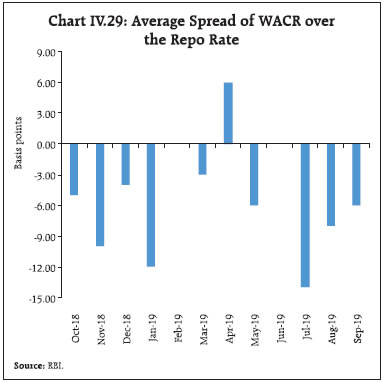 The WACR remained 6 bps above the policy repo rate (on an average) in April and below the policy repo rate by an identical margin in May. In June, however, it remained closely aligned with the policy repo rate (Chart IV.29). Subsequently, the WACR traded below the policy repo rate (on an average) by 14 bps in July, 8 bps in August and 6 bps in September. Overall, the WACR traded below the policy repo rate by 5 bps in H1:2019-20 as compared with 6 bps in H2:2018-19. IV.4 Conclusion Domestic financial markets remained vulnerable to global headwinds and geo-political uncertainties. After post-elections exuberance, equity markets turned risk averse reacting to global developments and slowdown in economic activity. Capital flows turned volatile in August, exerting depreciation pressures on currencies. By contrast, the bond market rallied significantly, despite some correction in the recent period. Credit growth, however, has slowed down, reflecting subdued economic prospects. Going forward, liquidity conditions would be managed consistent with the stated policy objective of aligning the WACR with the policy repo rate and ensuring that durable liquidity needs of the economy are adequately met, consistent with the stance of monetary policy. Ensuring faster monetary transmission to banks’ lending rates remains a key priority. _____________________________________________________________________
V. External Environment Global economic activity has remained sluggish as major advanced economies (AEs) and emerging market economies (EMEs) slowed down in Q2:2019. Mounting trade and geo-political uncertainties continue to cloud the near-term outlook. Monetary policy has been easing across the world to support growth concerns as inflation remains benign. Financial markets remained volatile on still unfolding sequence of US tariff actions and lingering uncertainty surrounding Brexit. Since the Monetary Policy Report (MPR) of April 2019, global economic activity has weakened and the near-term outlook remains clouded by trade and geo-political uncertainties. Most major AEs and EMEs slowed down in Q2:2019. Crude oil prices remained volatile on shifting demand-supply balances, most recently caused by supply disruptions in Saudi Arabia – the second largest oil exporter – estimated to be of the order of around 5 per cent of global oil supply. Other global commodity prices remained soft on subdued global demand. Central banks across the world eased monetary policy to support growth concerns as inflation remains benign. The calm that characterised global financial markets in the beginning of 2019 has been dispelled since May, with a combination of trade and geo-political tensions and the worsening global growth outlook imparting heightened volatility. V.1 Global Economic Conditions Economic activity has been losing pace across major AEs and EMEs. In the US, real GDP growth (q-o-q, annualised) decelerated in Q2:2019 to 2.0 per cent, after rebounding in Q1, on slumping exports and weak business fixed investment (Table V.1). Incoming data suggest that the slowdown may continue in Q3, as industrial production remains subdued and exports continue to decline. The Institute of Supply Management’s manufacturing index declined further into the contraction zone in September marking its lowest reading in a decade. Nonetheless, strong consumer spending, as reflected in rising retail sales, is expected to moderate the pace of slowdown to some extent. Euro area GDP growth slowed down in Q2:2019 as its major constituent economies lost steam amidst lingering uncertainties around Brexit and trade tensions. The German economy contracted in Q2 with a struggling auto industry amidst falling exports; it entered Q3 on a weak note as the manufacturing PMI in September remained in contraction zone, marking the ninth consecutive month of decline in factory activity. GDP growth in Italy stagnated in Q2 as contraction in industry and agriculture activities was offset by an uptick in the services sector, though its high level of debt and ongoing political uncertainty are downside risks. | Table V.1: Real GDP Growth (q-o-q, annualised) | | (Per cent) | | Country | Q2-2018 | Q3-2018 | Q4-2018 | Q1-2019 | Q2-2019 | 2019 (P) | 2020 (P) | | Advanced Economies | | Canada | 2.5 | 2.1 | 0.3 | 0.5 | 3.7 | 1.8 | 1.7 | | Euro area | 1.6 | 0.8 | 1.2 | 1.6 | 0.8 | 1.6 | 1.5 | | Japan | 1.9 | -1.9 | 1.8 | 2.2 | 1.3 | 0.2 | 1.4 | | South Korea | 2.4 | 2.0 | 3.6 | -1.6 | 4.0 | 2.6 | 2.8 | | UK | 2.0 | 2.4 | 1.2 | 2.4 | -0.8 | 1.2 | 1.6 | | US | 3.5 | 2.9 | 1.1 | 3.1 | 2.0 | 2.3 | 1.9 | | Emerging Market Economies | | Brazil | -0.4 | 2.0 | 0.4 | -0.4 | 1.6 | 1.3 | 2.5 | | China | 6.8 | 6.4 | 6.0 | 5.6 | 6.4 | 6.1 | 5.9 | | Malaysia | 2.4 | 6.0 | 5.2 | 4.4 | 4.0 | 4.6 | 4.8 | | Mexico | -0.8 | 2.0 | 0.3 | -1.0 | 0.1 | 1.3 | 1.6 | | Russia* | 2.2 | 2.2 | 2.7 | 0.5 | 0.9 | 2.0 | 1.0 | | South Africa | -0.5 | 2.6 | 1.4 | -3.1 | 3.1 | 1.0 | 0.3 | | Thailand | 4.3 | -0.9 | 3.6 | 4.1 | 2.4 | 3.9 | 3.7 | | Memo: | 2018 (E) | 2019 (P) | 2020 (P) | | World Output | 3.6 | 3.2 | 3.5 | | World Trade Volume | 3.7 | 2.5 | 3.7 | E: Estimate P: Projection *: y-o-y growth
Sources: Bloomberg; and International Monetary Fund (IMF). | The Japanese economy grew at a slower pace in Q2 than in the preceding quarter as escalating US-China trade tensions and slackening global demand prompted a sharp downward revision in business spending. Combined with a scheduled sales tax hike, this has clouded the economic outlook for the rest of 2019. Nonetheless, fiscal stimulus and rushed purchases ahead of the sales tax hike are expected to support the economy in Q3. Real GDP in the UK contracted in Q2 on the back of declining manufacturing activity due to planned early shutdowns of car plants in April following Brexit uncertainty. Risks from a potential hard Brexit deal and evolving global trading conditions cloud the near-term outlook. Economic activity remained subdued in key EMEs, held down by weakening global economic conditions. The Chinese economy decelerated in Q2 (y-o-y) to its weakest pace in nearly 27 years, weighed down by the adverse impact of the prolonged and unresolved trade dispute with the US, and subdued global demand. Available high frequency indicators suggest that the downtrend may continue, going forward. Industrial production and retail sales have declined since July, while the manufacturing PMI remains subdued amidst weak demand. While the overall risk remains titled to the downside on rising internal and external headwinds, policy stimuli on both the fiscal and monetary fronts are expected to cushion the pace of the slowdown. Among other BRICS economies, the Russian economy is struggling to regain momentum after undergoing a sharp deceleration in Q1. While economic activity showed a slight uptick in Q2, incoming data showed signs of weakness for Q3 as consumer sentiment remained subdued, with industrial production and retail sales weakening since July. Nonetheless, higher fiscal spending for national development projects may support aggregate demand, going ahead. The economies of Brazil and South Africa rebounded in Q2, after witnessing a sluggish start to the year. Economic recovery in Brazil was largely supported by strong fixed investment and construction activity in Q2. While improved sentiment amidst accommodative monetary policy is expected to sustain the expansion, risks from both domestic and external challenges may contain the momentum. In South Africa, economic activity accelerated on robust growth in mining and manufacturing, thus recouping output losses witnessed in Q1. The consumption-led economic recovery, however, is expected to be gradual as the uncertain global outlook and debt-ridden domestic power utilities may continue to weigh on the overall prospects of the economy. The Indonesian economy slowed down to 5.1 per cent (y-o-y) in each of the first two quarters of 2019, pulled down by subdued investment and declining exports, amidst global uncertainty. In Thailand, the downturn that had started in Q1 continued in Q2 (y-o-y), marking the slowest growth in nearly five years. The struggling farm sector, slowing exports and the weakening tourism sector resulted in the slowdown. The Turkish economy registered positive growth in the first half of 2019, recovering from last year’s recession caused by a currency crisis. The recovery was underpinned by the stimulus provided in Q1 through high government spending and credit expansion. The global composite PMI fell in August, after registering a marginal uptick in July, as slowing global trade weighed down on overall export growth (Chart V.1a). Among the major OECD economies, composite leading indicators (CLIs) point to a slowdown in growth momentum across major AEs and EMEs (Chart V.1b). The slowdown in global trade, which began in the later half of 2018, has continued in 2019, with contribution from EMEs slipping into contraction in 2019 (Chart V.2a). Forward looking indicators suggest that world trade is likely to slow down further in2019. The WTO’s Goods Trade Barometer1 remains below trend, driven by sluggish performance in all its constituent indices, especially international air freight, electronic components and automobile production. Movement in other indicators such as the Baltic Dry Index also remained sluggish, though with some signs of revival (Chart V.2b). V.2 Commodity Prices and Inflation Global commodity prices weakened as trade tensions intensified. The Bloomberg commodity price index declined by 4.1 per cent between April and September 2019. The food price index of the Food and Agriculture Organisation (FAO) increased by 1.4 per cent during April-September 2019. Global food prices rose for the fifth consecutive month in May, driven by high dairy and maize prices resulting from tighter export supplies. They, however, slid marginally in June-July as dairy prices fell on weak demand. Global food prices moderated further in August due to a sharp decline in cereals and sugar prices. While cereal prices fell on ample export supplies, weakening Brazilian currency and prospects of larger shipments by India and Mexico kept sugar prices low (Chart V.3a). Movements in global food prices have implications for food price inflation in EMEs (Box V.1). 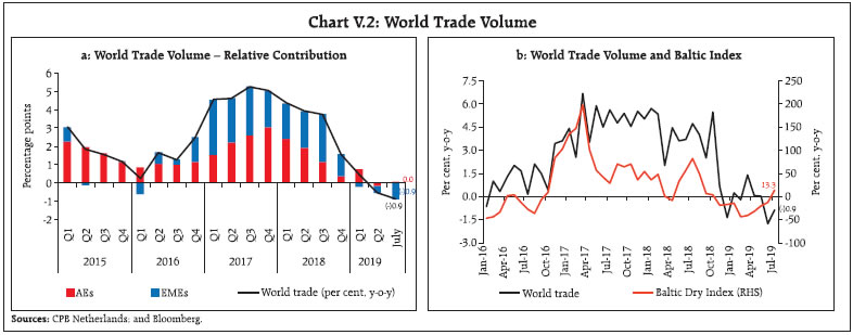 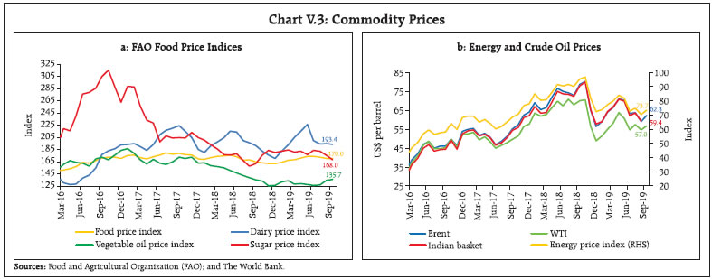 The stand-off between the US and Iran and agreement by key oil producers to extend supply cuts further by nine months exerted upward pressures on oil prices in early May. However, a decline in the expected demand for oil amidst adequate supplies eased market tightness and weighed on prices, before witnessing the biggest one-day gain on September 16, 2019, caused by supply disruptions to the world’s largest oil processing facility in Saudi Arabia. However, it eased thereafter on expectations of supply restoration (Chart V.3b). Base metal prices, measured by the Bloomberg base metal spot index, declined by 9.0 per cent between April and September 2019 on increased pessimism over the growth outlook and slowing global demand on persistent trade tensions. However, they recovered marginally in July on elevated supply concerns about iron ore and nickel by major exporters and have been trading side-ways thereafter, as the market awaits further developments on the trade front. Copper prices fell sharply on waning demand, triggered by trade uncertainties, with intermittent increases in June on a mine strike in Chile and weak Chinese refined copper output. Gold prices remained elevated on safe haven demand as global uncertainties increased (Chart V.4). Inflation remained benign in major AEs and EMEs. Among AEs, CPI inflation in the US remained tepid despite tight labour markets, as the sensitivity of inflation to levels of resource utilisation remains low. However, it registered a modest uptick in July on recovering energy prices. While core personal consumption expenditure (PCE) – the Fed’s preferred measure of inflation – has been picking up since June, it remains below the US Fed’s 2 per cent target. In the Euro area, inflationary pressures have been easing on soft energy costs and weakening growth. In Japan, CPI inflation remained muted amidst falling food, transport and communication prices (Chart V.5a). 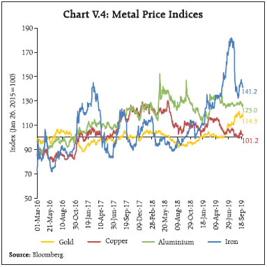
Box V.1: International Food Prices – Pass-through to EMEs International food prices have been among the most significant sources of domestic food price variations in many EMEs, as the share of food in household expenditure is relatively high in these countries. The World Bank’s food price index increased by 23.8 per cent in 2007, 33.5 per cent in 2008 and by 22.5 per cent in 2011, with unexpected spikes seen across all food groups. Although the magnitude of price increases in these episodes was almost the same, the affected commodities were different (Chart V.1.1). While rice, wheat, oil and cereal prices remained high during 2007-08, sugar prices remained low. Rice prices were the highest during the first episode but were lower than many other cereal products during the second episode. 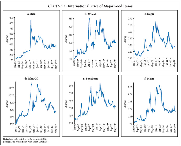 According to the Law of One Price (LOP) (Ardeni, 1989; Barahona and Chulaphan, 2017), in efficient markets for a single homogenous commodity, assuming no transport costs or obstacles to trade, prices expressed in a common currency are equated according to the following equation: where ER is the exchange rate [unit(s) of domestic currency per unit of foreign currency], Pw is the world (foreign) food price and Pd is the domestic food price. The estimable version of equation (1) can be modified as a weak LOP hypothesis which in natural logarithm form is as below: Pw is implicitly assumed to be an exogenous variable, as EMEs are generally price takers and β is the long-term price transmission elasticity in the presence of a long-run relationship. The short-term price elasticity can be estimated from the error correction model (ECM) of the following form: Where Δ is the first difference operator, ECT is the error correction term, φ and γ are the short-term transmission elasticities and ρ is the persistence parameter. Against this backdrop, the pass-through of changes in world food prices to domestic food prices was examined for six EMEs, viz., Brazil, China, India, Indonesia, Thailand and Turkey as these countries have a high share of food items in their consumer price indices (Sahoo et al., 2019). Using monthly data from January 2007 to July 2019, it was found that each of the variables, viz., global food price index, country-specific food price indices and exchange rates are integrated of order one, i.e., I(1). Therefore, the existence of a cointegrating relationship was examined through vector error correction model (VECM). The lag length of each model was based on Akaike Information Criteria (AIC). The estimated VECM model for each country confirms that residuals are not serially correlated. The estimated short-run and long-run transmission elasticities reveal that the magnitude of price transmission from world food prices to domestic food prices differs across countries (Table V.1.1). All the transmission elasticities are positive and different from zero and short-run elasticities are lower than the long-run elasticities, barring for Turkey and India. The short-run price transmission elasticity for food price in India is 0.05, implying that if world food price increases by one per cent, food CPI in India could increase by five basis points. | Table V.1.1: Estimated World Food Price Pass-through Coefficients | | Country | Long-run | Short-run | | Brazil | 1.136*** | 0.024* | | China | 0.179** | 0.029* | | India | 0.038*** | 0.054* | | Indonesia | 0.355*** | 0.082*** | | Thailand | 0.933*** | 0.040* | | Turkey | 0.055*** | 0.130*** | Note: ***, ** and * denote 1 per cent, 5 per cent and 10 per cent level of significance, respectively.
Source: RBI staff estimates. | To summarise, volatile food prices pose a significant policy challenge across the world and have implications for domestic inflation in EMEs, especially those having high share of food imports. References: Ardeni, P. G. (1989), “Does the Law of One Price Really Hold for Commodity Prices?”, American Journal of Agricultural Economics, 71(3), Vol. 71, no. 3, pp. 661-669. Barahona, J. F. and W. Chulaphan (2017), “Price Transmission between World Food Prices and Different Consumer Food Price Indices in Thailand”, Kasetsart Journal of Social Sciences, Available online at: https://www.sciencedirect.com/science/article/pii/S2452315117300206?via%3Dihub. Sahoo, S., S. Kumar and B. Gupta (2019), “International Food Prices – Pass-through to EMEs”, Reserve Bank of India (Mimeo). | Inflation has been easing in many EMEs. In Russia, inflation edged lower since Q2 as consumer demand remained weak, while easing supplies on a strong harvest and appreciating ruble have added to disinflationary conditions. In Brazil, CPI inflation has been falling since April on the back of soft food and fuel prices; however, it picked up marginally in August on rising housing and transport prices. In South Africa, inflation eased in July, after remaining steady in Q2 on falling fuel prices. In August, however, it edged up on rising food and housing prices. Inflation in Turkey, which has been ebbing since April, registered a sharp drop in June, driven by a favourable base effect and softening of food prices. In July, however, it showed a slight uptick on high service prices resulting from increased municipal tariffs, before resuming its downward path in August (Chart V.5b). V.3 Monetary Policy Stance Monetary policy has become accommodative across major AEs and EMEs. The US Fed has reduced its policy rate twice since July 2019 on concerns over lingering trade uncertainties and muted inflationary pressures (Chart V.6a). The European Central Bank (ECB) reduced the interest rate on deposit facility deeper into negative territory, while approving a fresh round of monetary stimulus in the form of bond purchases of 20 billion euros per month, beginning from November 2019. Ebbing inflation, waning business confidence and fears of Germany sliding into recession prompted the ECB to unveil another round of quantitative easing. The ECB has also indicated that rates will remain at present or lower levels until the inflation outlook converges to a level sufficiently close but below 2 per cent within its projection horizon. The Bank of Japan (BoJ) continued with its ultra-loose monetary policy on mounting downside risks to the economy and signalled a ramping up of stimulus if growth momentum loses further. The UK and Canada kept their policy rates unchanged, while South Korea kept its policy rate unchanged in August, after reducing it by 25 bps in its July meeting on concerns over slowing growth. Central banks in EMEs have turned increasingly dovish in sync with their AE counterparts on easing inflation conditions and weakening economic outlook. Among the BRICS, the People’s Bank of China (PBOC) continued with its loose monetary policy stance, while indicating potential policy adjustments, going forward, as the domestic situation warrants. Moreover, with the aim of stimulating the economy via ample liquidity conditions, the PBOC provided liquidity support to small and medium sized banks by increasing rediscount quota and standing lending facility to RMB 200 billion and RMB 100 billion, respectively, in June. In order to support the development of the real economy and lower financing costs, the PBOC lowered the required reserve ratio for financial institutions by 50 bps in September 2019 (excluding finance companies, financial leasing companies and auto finance companies). In an effort to increase the support for micro and small businesses, it has also decided to lower the required reserve ratio by 50 bps each on October 15 and November 15, 2019 for rural commercial banks operating solely within provincial administrative regions. Furthermore, it reduced its loan prime rate for one year maturity by 5 bps in its September meeting. 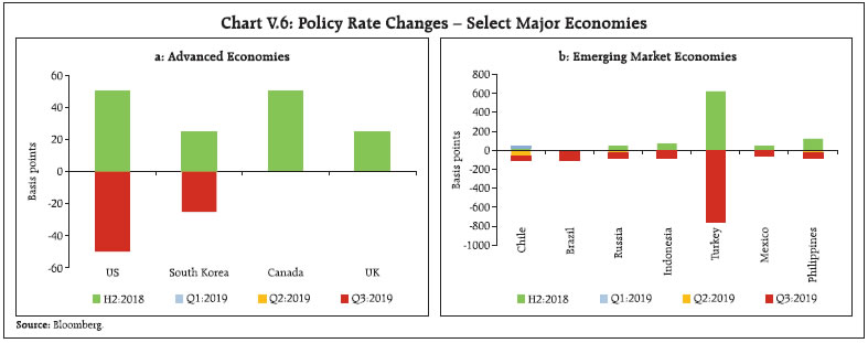 Brazil cut its policy rate twice since July, attributing it to moderating inflationary pressures and weakening economic activity. Russia reduced its policy rate thrice in 2019 on falling inflation and weak demand. South Africa held its policy rate in September, while reducing it in July amidst ebbing inflation expectations. Among other EMEs, Turkey slashed its policy rate by 425 bps and 325 bps in July and September, respectively, exceeding market expectations, as the improving inflation outlook provided more space for policy easing. The Philippines reduced its policy rate for the third time in 2019 in its September meeting with a view to reviving business investment and supporting slowing economy. Mexico reduced its policy rate in September, making it the second consecutive cut since August. Chile has reduced its policy rate twice since June. Indonesia reduced its policy rate by 25 bps in its September meeting, making it the third consecutive cut in Q3:2019, for boosting economic growth amidst low inflation (Chart V.6b). V.4 Global Financial Markets Financial markets remained volatile as sentiment was repeatedly impacted by the still unfolding sequence of US tariff actions and lingering uncertainty surrounding Brexit. Global equity markets witnessed sharp sell-offs in May reversing the gains till April. However, markets recouped most of the losses in June-July as sentiment was buoyed by dovish guidance by major central banks and renewed hopes of trade truce, before declining again in August as unresolved and intensifying trade dispute triggered bearish sentiment. In September, positive signals on trade negotiations buoyed investors’ risk appetite. Bond yields eased across major economies on safe haven demand, while currency markets remained volatile. Among AEs, US equities gained in June-July, after correcting in May, driven by resilient corporate earnings data for Q1:2019 and rising expectations of monetary policy easing by the Fed in the coming months. In August, while increasing risk-off sentiment amidst intensifying trade tensions and growth worries led to large sell-offs, positive developments on the trade front revived market sentiment in September, as a result of which equity markets recovered most of its losses suffered in August. In the Euro area, equity markets tumbled in May in response to weak German data. However, they remained supported in June-July on expectations of monetary policy accommodation by the ECB and positive developments in earning expectations for non-financial corporations. Nonetheless, markets ended August on a soft note as growth worries resurfaced on weak German data and political turmoil in Italy. Japanese equity markets also firmed up in June-July after correcting in May. Markets maintained an uptrend in July as trade concerns receded, though they plunged in the middle of the month on appreciation of the Yen and concerns over deteriorating performance of some exportoriented companies. Equity markets in AEs entered September on a positive note as global investors’ sentiment was lifted on reduced tensions in Hong Kong and renewed hopes of trade negotiations. Stock markets in EMEs fell as the strong US dollar acted as a headwind leading to capital outflows. Weak South Korean equities following trade conflicts with Japan, political unrest in Hong Kong, crash in Argentina’s financial markets and escalating trade tensions pulled down EME stocks further in August. However, some of the losses were recovered subsequently as market sentiments were boosted by postponement of tariff imposition and signals of stimulus for the Chinese economy (Chart V.7). Bond yields have eased across major AEs and EMEs as investors looked for safe havens on waning risk appetite. US bond yields softened in May, after picking up in April on better GDP data for Q1. They have declined sharply since then, even falling below 2 per cent in August amidst heightened trade tensions and dovish stance of the US Fed. A sharp fall in long-term yields has led to a negative yield spread between 10-year and 3-month Treasury securities, as addressed in Box I.1 in chapter I. In the Euro area, bond yields plunged into negative territory in most of its constituent economies as expectations of dovish monetary policy stance by the ECB gained traction, amidst a weakening economic outlook. Lacklustre data for Germany and political uncertainties in Italy added further downward pressure. In Japan, bond yields continued to trade in negative territory on subdued risk appetite. In most EMEs, bond yields have been falling, with central banks becoming highly accommodative as benign inflation has freed up policy space to boost slackening economic growth (Chart V.8a). 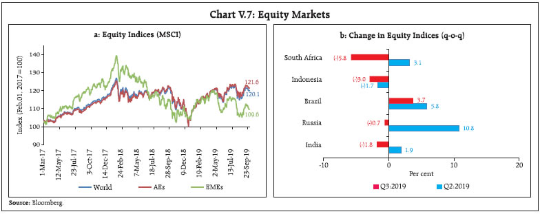 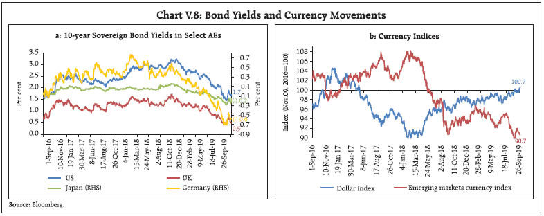 In currency markets, the US dollar weakened against major currencies in June on dovish guidance by the US Fed but it has rebounded since July, recouping most of its losses made in Q1. Safe haven demand amidst weaker growth prospects in other AEs also strengthened the US dollar. The euro lost ground against the US dollar as the economy lost momentum, while higher probability of the ECB to stimulate the economy pulled the currency further down. The Japanese yen outperformed most of the major currencies as trade war induced uncertainties, coupled with worsening global growth conditions, played up investors’ risk-off sentiments. Most of the EME currencies suffered losses against the strong US dollar and mounting spillover risks arising from trade tensions. Between April and September 2019, the MSCI Emerging Market Currency Index declined by 2.0 per cent (Chart V.8b). V.5 Conclusion In sum, global economic activity continues to lose momentum as prolonged uncertainties relating to geo-political developments dampened economic sentiment. With inflationary pressures remaining benign and market sentiment remaining fragile, risks to the global outlook remain on the downside. However, monetary and fiscal stimuli across the globe may help in containing the pace of slowdown and putting the global economy on a recovery path. ________________________________________________________________
ABBREVIATIONS | AEs | Advanced Economies | | AIC | Akaike Information Criteria | | AIFIs | All India Financial Institutions | | BAI | Business Assessment Index | | BE | Budget Estimates | | BEI | Business Expectations Index | | BK | Baxter-King | | BoJ | Bank of Japan | | Bps | Basis Points | | BRICS | Brazil, Russia, India, China and South Africa | | BS-IV | Bharat Stage - IV | | BSE | Bombay Stock Exchange | | CAD | Current Account Deficit | | CAG | Comptroller and Auditor General of India | | CD | Certificate of Deposit | | CDS | Credit Default Swap | | CF | Christiano-Fitzgerald | | CGA | Controller General of Accounts | | CGST | Central Goods and Service Tax | | CiC | Currency in Circulation | | CI | Confidence Interval | | CII | Confederation of Indian Industry | | CLI | Composite Leading Indicator | | CMB | Cash Management Bill | | CMIE | Centre for Monitoring Indian Economy | | CP | Commercial Paper | | CPC | Central Pay Commission | | CPI | Consumer Price Index | | CPI-C | Consumer Price Index - Combined | | CPI-AL | Consumer Price Index for Agricultural Labourers | | CPI-IW | Consumer Price Index for Industrial Workers | | CPI-RL | Consumer Price Index for Rural Labourers | | CRR | Cash Reserve Ratio | | CU | Capacity Utilisation | | CU (SA) | Capacity Utilisation (Seasonally Adjusted) | | DEA | Digestive enzymes and antacids | | DGCA | Directorate General of Civil Aviation | | DGCI&S | Directorate General of Commercial Intelligence and Statistics | | DM | Dynamic Multiplier | | ECB | European Central Bank | | ECRI | Economic Cycle Research Institute | | ECM | Error Correction Model | | ECT | Error Correction Term | | EMs | Emerging Markets | | EMEs | Emerging Market Economies | | EU | European Union | | FAE | First Advance Estimates | | FAO | Food and Agriculture Organisation | | FBIL | Financial Benchmarks India Pvt. Ltd | | FCCBs | Foreign Currency Convertible Bonds | | FDI | Foreign Direct Investment | | FIs | Financial Institutions | | FICCI | Federation of Indian Chambers of Commerce and Industry | | FMCG | Fast-Moving Consumer Goods | | FPI | Foreign Portfolio Investment | | FRE | First Revised Estimates | | FX | Foreign Exchange | | FY | Financial Year | | GARCH | Generalized Autoregressive Conditional Heteroskedasticity | | GDP | Gross Domestic Product | | GFCE | Government Final Consumption Expenditure | | GFCF | Gross Fixed Capital Formation | | GFD | Gross Fiscal Deficit | | GIC | General Insurance Corporation | | GIC HFL | GIC Housing Finance Limited | | GNDI | Gross National Disposable Income | | GOI | Government of India | | G-Secs | Government Securities | | GST | Goods and Services Tax | | GSTN | Goods and Services Tax Network | | GVA | Gross Value Added | | H1 | First Half of the Year | | H2 | Second Half of the Year | | HDFC | Housing Development Finance Corporation | | HFC | Housing Finance Company | | HP | Hodrick-Prescott | | HRA | House Rent Allowance | | ICR | Interest Coverage Ratio | | IEA | International Energy Agency | | IGST | Integrated Goods and Service Tax | | IIP | Index of Industrial Production | | IL&FS | Infrastructure Leasing and Financial Services Limited | | IMD | India Meteorological Department | | IMF | International Monetary Fund | | IMO | International Maritime Organisation | | INR | Indian Rupee | | IOCL | Indian Oil Corporation Limited | | IOS | Industrial Outlook Survey | | IRF | Impulse Response Function | | ISMA | Indian Sugar Mills Association | | IT | Information Technology | | LAF | Liquidity Adjustment Facility | | LCR | Liquidity Coverage Ratio | | LIBOR | London Inter- bank Offered Rate | | LIC | Life Insurance Corporation of India | | LIC HFL | LIC Housing Finance Limited | | LOP | Law of One Price | | LPA | Long Period Average | | LPG | Liquefied Petroleum Gas | | MA | Moving Average | | Mb/d | million barrels per day | | MEIS | Merchandise Export from India Scheme | | MCLR | Marginal Cost of Funds Based Lending Rate | | MFs | Mutual Funds | | MIBOR | Mumbai Interbank outright Rate | | m-o-m | Month-on-Month | | MPC | Monetary Policy Committee | | MPR | Monetary Policy Report | | MSCI | Morgan Stanley Capital International | | MSF | Marginal Standing Facility | | MSMEs | Micro, Small and Medium Enterprises | | MSP | Minimum Support Price | | MVKF | Multivariate Kalman Filter | | NAFED | National Agricultural Cooperative Marketing Federation of India | | NBER | National Bureau of Economic Research | | NBFCs | Non-Banking Financial Companies | | NCAER | National Council of Applied Economic Research | | NDSI | Non-Deposit Systemically Important | | NDS-OM | Negotiated Dealing System-Order Matching | | NDTL | Net Demand and Time Liabilities | | NEER | Nominal Effective Exchange Rate | | NFC | Non-Food Credit | | NHB | National Housing Bank | | NIIP | Net International Investment Position | | NPA | Non-Performing Asset | | NSC | National Savings Certificate | | NSDL | National Securities Depository Limited | | NSE | National Stock Exchange | | NSO | National Statistical Office | | OBICUS | Order Books, Inventories and Capacity Utilisation Survey | | OD | Over Draft | | OECD | Organisation for Economic Co-operation and Development | | OG | Output Gap | | OIS | Overnight Indexed Swap | | OMCs | Oil Marketing Companies | | OMOs | Open Market Operations | | OPEC | Organisation of the Petroleum Exporting Countries | | PADO | Public Administration, Defence and Other Services | | PBOC | People’s Bank of China | | PCE | Personal Consumption Expenditure | | PD | Primary Dealer | | PE | Provisional Estimates | | PFCE | Private Final Consumption Expenditure | | PMI | Purchasing Managers’ Index | | POL | Petroleum, Oil, and Lubricants | | PMUY | Pradhan Mantri Ujjwala Yojana | | PRN | Production Weighted Rainfall Index | | PSBs | Public Sector Banks | | PSU | Public Sector Undertaking | | Q1 | First Quarter | | Q2 | Second Quarter | | Q3 | Third Quarter | | Q4 | Fourth Quarter | | q-o-q | Quarter-on-Quarter | | RBI | Reserve Bank of India | | RD | Revenue Deficit | | RE | Revenue Expenditure/Revised Estimate | | REER | Real Effective Exchange Rate | | RHS | Right Hand Side | | RMB | Renminbi | | RMSE | Root Mean Squared Error | | SAAR | Seasonally Adjusted Annualised Rate | | SAE | Second Advance Estimates | | SCBs | Scheduled Commercial Banks | | SDLs | State Development Loans | | SEBI | Securities and Exchange Board of India | | SGST | State Goods and Service Tax | | SIAM | Society of Indian Automobile Manufacturers | | SLR | Statutory Liquidity Ratio | | SVAR | Structural Vector Autoregression | | T-Bill | Treasury Bill | | TLTRO | Targeted Longer-term Refinancing Operations | | TVP-VAR | Time-Varying Parameter Vector Autoregression | | UK | United Kingdom | | US | United States | | US$/USD | US Dollar | | VAR | Vector Autoregression | | VARX | Vector Auto Regression with Exogenous Variables | | VECM | Vector Error Correction Model | | VIX | S&P 500 Volatility Index | | VRR | Voluntary Retention Route | | WACR | Weighted Average Call Money Rate | | WADR | Weighted Average Discount Rate | | WADTDR | Weighted Average Domestic Term Deposit Rate | | WALR | Weighted Average Lending Rate | | WMA | Ways and Means Advances | | WPI | Wholesale Price Index | | WTI | West Texas Intermediate | | WTO | World Trade Organisation | | WTOI | World Trade Outlook Indicator | | y-o-y | Year-on-Year | | YTM | Yield to Maturity | |