Committed expenditures on account of pay commission award and interest payments coupled with expenditures coming from state-specific schemes like farm loan waivers have been generating pressures on state budgets. Reducing leakages and enhancing efficiency of public distribution system coupled with improved public financial management practices may be necessary to rebuild fiscal space. Market borrowings provide an easy access to finance for states, but the present lack of incentives to undertake fiscal reforms so as to lower borrowing spreads could add to the debt sustainability concerns of the states going forward.

1. Introduction

3.1 This chapter drills down into issues confronting states on the expenditure side, especially committed expenditures and funding aspects, including market access. States’ own revenue to GDP ratio grew by 6.7 per cent on average during the 1990s and by 7.2 per cent during 2000s so far. At the same time, committed expenditures (as per cent to GDP) have expanded at a faster pace during this period right up to 2017-18 (Chart II.3 in Chapter II).

3.2 Against this backdrop, Sections 2 to 4 delve into specific issues on the expenditure side, viz., implementation of the pay commission’s awards, farm loan waivers, and food security subsidies. While these additional claims on state expenditures are on a rise, fiscal marksmanship on the part of the states has been rather weak, raising questions about their credibility. Section 5 extends the analysis of consolidated states’ finances undertaken in the preceding state finance reports (RBI, 2015 and RBI, 2017) and applies globally employed quantitative indicators on individual state data to assess fiscal marksmanship of states. Section 6 explores issues surrounding market access of states through state development loans (SDLs) which will increasingly determine their fiscal space going forward. Concluding observations are given in Section 7.

2. State Pay Commission Awards

3.3 Wages and salaries constitute a significant portion of the committed liabilities of states, accounting for 23.6 per cent of their combined revenue expenditure in 2016-17, followed by pensions (10.8 per cent). The seventh central pay commission (CPC) recommended revisions in the salary and other emoluments, including housing rent allowance (HRA). Some states follow their own pay commission rules while others follow CPC rules. Moreover, implementation has not been either uniform or complete. Although states like Jharkhand, Bihar, Chhattisgarh, Madhya Pradesh and Tamil Nadu have implemented their pay commission awards from January 2016 in line with the seventh CPC, actual payments for most of these states were made in 2017-18. As regards arrear payments, most of the states have provided for staggering them over a two-three year period (Table III.1).

3.4 Some other states like Assam, Karnataka, Meghalaya, Nagaland, Tripura, Telangana and Kerala revise their emoluments from time to time as per their own pay commission rules. Assam, Karnataka, Meghalaya, Nagaland and Tripura have effected pay revisions in 2017-18.

3.5 Committed expenditure under this head may have a bearing on the fiscal balance of 12 states in 2017-18 and nine states in 2018-19, with payment of arrears getting stretched to 2019-20 and 2020- 21 for a few of them. For states that have started implementing the pay commission award in 2017-18, there is a growth of about 28 per cent in revenue expenditure in 2017-18 (RE), particularly for the non-special category states as against all-states average growth of about 20 per cent (Chart III.1).

3.6 Within revenue expenditure, the growth in wages and salaries has been particularly sharp in 2017-18 (RE) for the states that have implemented pay commission awards (Chart III.2).

3.7 Estimates suggest that while the fifth CPC had a cumulative impact of 1.0 per cent of GSDP over a two year period -1999-2000 to 2000-01 (Mohan, 2008) - the impact of the sixth CPC on state finances was about 1.4 per cent of GSDP over a two-year period (Kumar and Krishna, 2015). Early estimates for seventh CPC on combined government finances over the duration of the fourteenth Finance Commission (FC-XIV) indicated an average impact of 0.9 per cent of GDP on revenue and fiscal deficits, premised on the assumption of a growth of 15 per cent in other revenue expenditures for 2016-17 - the year of implementation of seventh CPC award (Bhanumurthy et al., 2015).

3.8 All states taken together are bigger employers than the centre. Furthermore, most states do not fulfil the norm of salary expenditure not exceeding 35 per cent of revenue expenditure (excluding interest payments and pensions) recommended by the thirteenth Finance Commission (FC-XIII)¹. During 2017-18 (RE) the share of expenditure on wages and salaries in revenue expenditure of states (net of interest payments and pensions) ranged from 19.1 per cent to 54.6 per cent after the pay revisions were implemented.

3.9 Out of a total slippage of 13 basis points in the consolidated revenue expenditure of all states in 2017-18 (RE as compared with BE), available estimates from 11 states that implemented pay revisions show that wages and salaries² contributed around 5 basis points. By staggering the payments over two to three years, states have strategically tried to contain the impact on fisc on this account. However, with arrears payments being staggered over the next three years (2018-19 to 2020-21), some pressure on state budgets on this account is likely to remain.

3. Agricultural Debt Waiver

3.10 Among the factors responsible for fiscal stress in certain states are farm loan waivers that have been announced since 2014, often justified on the grounds of falling prices of agricultural commodities and recurring droughts. The debt waiver schemes of Andhra Pradesh and Telangana announced in 2014 were to the tune of ₹240 billion (4.6 per cent to GSDP) and ₹170 billion (3.4 per cent to GSDP), respectively, while Tamil Nadu loan waiver scheme of 2016 amounted to ₹60 billion (0.5 per cent to GSDP)³. In 2017, Maharashtra, Uttar Pradesh and Punjab sanctioned farm loan waivers to the tune of ₹340 billion (1.3 per cent of GSDP), ₹360 billion (2.7 per cent of GSDP) and ₹100 billion (2.1 per cent of GSDP), respectively. Rajasthan followed suit with a debt waiver announcement of ₹80 billion in February 2018 amounting to 0.9 per cent of GSDP. Karnataka, in the recently released budget 2018-19 (July 2018), announced farm debt waiver of ₹340 billion (2.4 per cent of GSDP)⁴.

3.11 The total debt waiver granted during 2017-18 amounted to 0.32 per cent of GDP as per revised estimates as opposed to budget estimates of 0.27 per cent of GDP. Total debt waivers are budgeted at 0.2 per cent of GDP during 2018-19.

3.12 The impact on states’ exchequers varies widely across the waiver implementing states, ranging between 4.6 per cent of GFD in Tamil Nadu to 60.9 per cent of GFD in Uttar Pradesh during 2017-18. As percentage of states’ GSDP, loan waivers were placed in the range of 0.1 - 1.9 per cent during 2017-18 (RE). According to 2018-19 budget estimates, states have allocated between 0.1 to 0.8 per cent of GSDP to loan waivers, amounting to 2.0 to 29.8 per cent of their budgeted GFD (Chart III.3). At a consolidated level, about a third (5 basis points) of the overall fiscal slippage of 13 basis points in revenue expenditure during 2017-18 (RE) may be attributed to loan waivers (see Chapter II).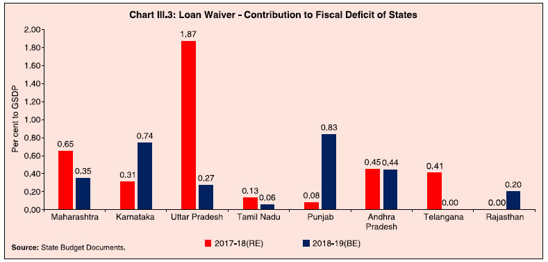

3.13 Since the actual waivers granted by states during 2017-18 have been below the announced/budgeted levels, it is likely that the pending debt waiver promises would spill over into coming fiscal years and continue to squeeze fiscal space. The decline in capital outlay growth during 2017-18 in some waiver granting states is a pointer to the likely impact of the waiver on developmental expenditure.

3.14 Debt waivers can deflect the state from its fiscal consolidation path, coming as they do, on top of UDAY and the implementation of the pay commission recommendations. Farm productivity enhancement through pecuniary incentives like debt waivers is unproven. Hence, higher fiscal deficits in future may not be offset by higher GDP gains. If the waivers are not targeted efficiently, coupled with structural productivity constraints in the farm sector, the potential for these waivers contributing to inflationary pressures via higher fiscal deficits remains a key concern (RBI, 2017).

3.15 Past experiences with loan waivers (Agricultural Debt Waiver and Debt Relief Scheme (ADWDRS of 2008) show that debt relief helps in reducing household debt but there appears to be no evidence of increase in investment and productivity of beneficiary households. Farmers may tend to factor in future credit constraints and reluctance of formal institutions to lend to them following waivers, and in turn, they may tend to shift to informal sources of credit (Kanz, 2016). Where debt waiver is given to farmers differentially, i.e., on the basis of their land holdings, the probability of obtaining credit post waiver was found to be higher for non-beneficiary farmers than for beneficiary farmers in the year of implementation of debt waivers (Box III.1).

Box III.1: Impact of Agricultural Loan Waivers – The Tamil Nadu Experience In June 2016, the newly elected Government of Tamil Nadu announced the waiver of agricultural loans for small and marginal farmers by state co-operative banks/ societies. The scheme waived crop loans, medium-term and long-term agricultural loans availed by small and marginal farmers which were outstanding in the books of co-operative societies as on March 31, 2016. Farmers with land holdings above 5 acres were not eligible for the waiver benefit. The cost to the state exchequer on account of the debt waiver scheme was ₹60.41 billion, of which an amount of ₹31.69 billion was to be paid to the cooperative institutions over a five-year period from 2016-17 to 2020-21. This includes interest at 8 per cent for phased reimbursement. In order to understand the impact of Tamil Nadu debt waiver scheme on the beneficiary farmers, transaction level accounts of agricultural credit given to all farmers for three years 2015-16, 2016-17 and 2017-18 (up to December 15, 2017) have been analysed (Raj and Prabu, 2018). Data were collected from 22 Primary Agricultural Cooperative Credit Societies (PACCS) in seven districts of Tamil Nadu. The objective was to ascertain, through the use of regression discontinuity design, whether there has been any significant difference between beneficiary farmers (acre <= 5) and non-beneficiary farmers (acre > 5) in access to short-term agricultural credit post-waiver. In this design, acreage (x) is taken to be the running variable, as the size of the land holding determined whether the farmer gets the debt waiveror not. The treatment, i.e., Di is taken to be equal to 1 for the beneficiary farmer and 0 for non-beneficiary farmer. Yi(1) is the outcome under treatment and Yi(0) is the outcome under control. The regression discontinuity (RD) design states that under the assumption that conditional mean of Yi(0) and Yi(1) are functions of acreage (x) and are continuous at the cut off (i.e., acre at 5), the average treatment effect between the beneficiary farmers vis-à-vis non-beneficiary farmers near the cut off can be measured as: The average treatment, i.e., obtaining credit after debt waiver is estimated using a local linear model (p = 1) to avoid over fitting with triangular kernel weights and employing coverage error rate bandwidth (Calonico et al., 2018). The empirical findings suggest that in the year of implementation, the probability of obtaining credit post-waiver is higher for non-beneficiary farmers who are just above the cut off acreage of 5 acres than for beneficiary farmers who are just below the cut off (Table 1; Chart 1). Intuitively this is due to (a) the time taken to verify the eligible farmer accounts which delayed the sanction of new loans to beneficiary farmers in the year of implementation of debt waiver; (b) non-beneficiary farmers being encouraged to make prompt repayment of crop loans to avail full interest relief5 with the promise of new loans; (c) reduction in recyclable funds of cooperative banks due to phased reimbursement of loan waiver amount; and (d) increase in new borrowers post waiver, mostly in the small and marginal farmer category; (e) restricted credit flow in November-December 2016 due to cash withdrawal limits placed during the period of withdrawal of legal tender of specified bank notes (SBNs). However, the differentiation in post-waiver access to credit to the beneficiary farmer and the non-beneficiary farmer comes down as the supply of funds for agricultural loans normalise. Table 1: Regression Discontinuity Effect of Obtaining Credit after Debt Waiver with Coverage Error Rate Optimal Bandwidth   Either Periods (2016-17 or 2017-18) 2016-17 2017-18 (Up to December 15, 2017) Average Treatment Effect (ATE) 0.083 *** 0.076 *** 0.187* 0.186* -0.010 -0.017 Standard Error 0.048 0.047 0.054 0.048 0.037 0.077 Pr(>|Z|) 0.082 0.082 0.000 0.000 0.921 0.943 Clustered No Yes No Yes No Yes Note: *, ** and *** represents significance at the standard 1%, 5% and 10% confidence intervals. Reference Calonico, S., M. D. Cattaneo, and M. H. Farrell, (2018), “On the Effect of Bias Estimation on Coverage Accuracy in Nonparametric Inference”, Journal of the American Statistical Association, forthcoming. DOI:https://doi.org/10.1080/01621459.2017.1285776

3.16 While waivers may cleanse banks’ balance sheets in the short term, it may disincentivise banks from lending to agriculture in the long term (EPW Research Foundation 2008; Rath 2008). Consequently, loan waivers can have a dampening impact on rural credit institutions. Moreover, they impact credit discipline, vitiate credit culture and dis-incentivise borrowers to repay loans, thus engendering moral hazard (De and Tantri, 2017). Besides, it may not just be loan waivers that are detrimental to the government balance sheet; it is the fiscal volatility emanating from random policy shocks that can have an even more enduring impact (Manna, 2017).

4. Rationalisation of Public Distribution System - National Food Security Act (NFSA), 2013

3.17 The public distribution system (PDS) in India is a collaborative effort of the central and state governments to provide food security. With the enactment of the NFSA, 2013 on September 10, 2013, India launched its most ambitious food security programme centred on the “right to food”. The NFSA marks a paradigm shift – from the welfare approach to a rights-based approach – in addressing the problem of food security by ensuring people’s access to adequate quantity of quality food at affordable prices. Over a span of about three years, i.e., between September 2013 and November 2016, all states have implemented the NFSA covering 807 million persons out of an intended coverage of 813 million persons accounting for two-thirds of the country’s population as per the 2011 census (Annex III.1).

3.18 The Act is being implemented in cash transfer mode in Chandigarh, Puducherry and in urban areas of Dadra and Nagar Haveli under which cash is credited to the bank accounts of beneficiaries who have the choice of buying foodgrains from the open market. The Act provides for a legal entitlement for 75 per cent of the rural population and 50 per cent of the urban population to receive 5 kilogrammes (kg) of foodgrains per person per month⁶ at subsidised prices (Table III.2).

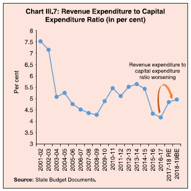
3.19 The NFSA stipulates that the issue price to the consumer cannot exceed the central issue price (CIP) for Antyodaya Anna Yojana (AAY) and priority household (PHH) categories although the states can fix prices lower than the CIP, while bearing the associated costs. Additional foodgrains are made available by the central government to those states which have lower regular allocation under NFSA as compared with the erstwhile targeted public distribution system (TPDS)⁷.

4.1 Food subsidy and its implications

3.20 Although food subsidy is primarily borne by the central government, with its share in total food subsidy averaging around 85 per cent during 2015-16 to 2017-18, state governments play an important role in food security as they are vested with the responsibility of distributing the subsidised foodgrains. The major subsidy from the centre is provided to the Food Corporation of India (FCI), its nodal agency for procurement and distribution of foodgrains under NFSA and other welfare schemes as well as for maintaining the buffer stock. State governments have been actively involved in the procurement and distribution of foodgrains since the introduction of the decentralised procurement scheme (DCP) by the central government in 1997-98.

3.21 The DCP scheme envisages (i) enhancing procurement of foodgrains in non-traditional states so as to ensure that the benefit of the MSP is passed on to local farmers; (ii) procurement of foodgrains that is more suited to local taste for distribution under PDS; and (iii) improving efficiency of PDS by saving on transit losses and costs. Notwithstanding the reluctance of some states to adopt the DCP mode in view of substantial responsibility in terms of financial and manpower resources⁸, the number of states/UTs procuring rice/wheat under the DCP mode have been rising over the years, and at present, there are 17 DCP states. Correspondingly, the share of central food subsidy to state agencies has increased from 11.2 per cent in 2007-08 to 26.6 per cent in 2017-18 (Chart III.4).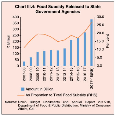

3.22 Before the introduction of the NFSA, some states were operating their own schemes which were providing benefits beyond the provisions of the NFSA. These benefits have continued even after the introduction of the NFSA. Some states have started their own food subsidy schemes co-terminus with or after the implementation of NFSA, as the Act allows for it. Accordingly, state-level food subsidies may arise due to the following factors: (a) issue price of foodgrains at the fair price shop is lower than the central issue price given to the states; (b) coverage in terms of persons entitled to subsidised food items under the food security scheme of the state is wider than mandated by the NFSA; and (c) coverage in terms of subsidised commodities provided through the public distribution system is wider than the ambit of the NFSA.

3.23 Eleven states offer foodgrains at prices lower than the cost at which they are acquired, i.e., the central issue price (CIP), of which three states, viz., Tamil Nadu, Karnataka and Kerala, distribute foodgrains free of cost to all AAY and PHH card holders, resulting in subsidy on this count (Chart III.5). It may be noted that the price subsidy will be higher for states which have a wider beneficiary coverage than envisaged under NFSA as they will have to procure additional foodgrains over and above the NFSA allocation at open market rates which are more than eight times the CIP for regular allocation and three times the CIP for tide-over allocation.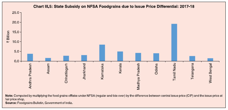

3.24 Besides subsidised foodgrains and sugar from the centre, some states/UTs have taken the initiative to distribute additional items of mass consumption through the PDS outlets such as pulses, edible oils and iodised salt at subsidised rates so as to make these more affordable and thus, meet the nutritional requirement of the people (Table III.3).

3.25 During 2015-16 to 2017-18, state level subsidies were in the range of 0.03- 0.43 per cent of the respective GSDP on average. While the operating cost of the NFSA is shared between the centre and the states, the additional schemes/items clearly represent a liability for respective state governments, which adds to their overall food subsidy burden. The average state food subsidy for 15 states was 0.22 per cent of their GSDP (0.14 per cent of GDP) during 2015-16 to 2017-18.

4.2 Strengthening and improving the efficiency of PDS

3.26 Although implementation of NFSA provided an opportunity to rectify inclusion and exclusion errors in the old below poverty line (BPL) lists, it was found that some major states which had implemented the NFSA included all old targeted public distribution system (TPDS) beneficiaries⁹. Inappropriate identification gives rise to high inclusion errors due to (i) non-poor households that were part of the old BPL list continuing in the new priority household list; and/or (ii) beneficiaries who were poor at the time of drawing the old list continuing to appear in the new list even after an improvement in their economic status.

3.27 The PDS in several states is plagued by problems of large leakages during transportation and distribution. Plugging these leakages can thus, lead to considerable savings to both the central and state exchequers. Based on inspections undertaken by states/UTs during 2015 to 2017, action has been taken on 30,432 fair price shops (FPS) for various irregularities (Government of India, 2018)¹⁰.

3.28 It is in this regard that the implementation of associated institutional reforms in states as required by the NFSA assumes importance. Considerable progress has been made in some of the institutional reforms, with all states/UTs achieving digitisation of ration cards/beneficiary data, setting up of transparency portals and establishment of grievance redressal mechanism. Automation of supply chain management has been completed in 20 states/UTs and online allocation of foodgrains has commenced in 30 out of the 35 states/UTs. Furthermore, seeding of Aadhaar cards of beneficiaries with their ration cards is being undertaken, with 81.9 per cent of all ration cards having been seeded up to January 30, 2018 to improve the delivery mechanism.

3.29 Notwithstanding the progress made so far, there is scope for the physical and institutional infrastructure to be strengthened further. Pre-requisites for the use of Aadhar-enabled Point of Sale (PoS) machines include high speed internet connectivity, uninterrupted power supply, good quality PoS devices and training for all stake holders in the TPDS process. Awareness campaigns about the grievance redressal mechanisms set up by the state governments in conjunction with local NGOs and self-help groups could help to improve the delivery mechanism. Furthermore, states could allocate more budget to maintain the monitoring system of the PDS. This initial increase in costs to the state exchequer would get smoothened over time with the reaping of long run benefits of a more efficient PDS (NCAER, 2015).

4.3 Cash Transfers: An alternative to PDS?

3.30 Direct benefit transfers (DBTs) through cash transfer of food subsidies reduce the need for large physical movement of foodgrains. Further, given the wide inter-state and intra-state variations in food consumption habits, DBTs provide greater autonomy to beneficiaries to choose their consumption basket and thereby enhance dietary diversity. However, a switch to cash transfers requires the fulfilment of certain pre-conditions as specified in the Cash Transfer of Food Subsidy Rules, 2015 of the Government of India. They include complete digitisation and de-duplication of the beneficiary database; seeding of bank account details and Aadhaar numbers in the digitised database; ensuring adequate availability of foodgrains in the open market; and identification of a state agency with a separate bank account to receive and transfer the subsidy to the bank accounts of the entitled beneficiaries. The Government of India has also released the Handbook for Implementation of Cash Transfer of Food Subsidy in May 2018, which lays down the requirements, timelines and best practices in cash transfers.

3.31 States desirous of shifting to DBT for food will have to make the transition to cash transfers cautiously to avoid problems experienced by DBT-operating UTs, such as inadequacy of transfers to maintain pre- DBT consumption levels, insufficiency of last-mile delivery mechanisms and weak grievance redressals. States with lower literacy levels, higher portion of below poverty line populations and relatively high child malnutrition could first strengthen the existing PDS through Information and Communication Technologies (ICT)-based in-kind transfers before embarking on ICT-based DBT cash transfers¹¹. Selective implementation in a few districts that exhibit diverse food habits and market infrastructure may be undertaken by states which have fulfilled the pre-conditions and feedback from these districts can be used to extend this programme further. To sum up, the PDS has been undergoing transformation and the state governments may have to be ready to adjust to the change to improve the efficiency of expenditure on providing food security to their people.

5. Credibility of State Budgets

3.32 Poor predictive power of estimates vis-à-vis actual outcomes has been a feature of state budgets. Assessment of fiscal marksmanship¹² of states, generally at the consolidated states’ level, exhibits a large systematic component in some of the expenditure items, particularly capital outlays, reflecting expedient adjustments necessitated by unanticipated shortfalls in meeting committed targets (RBI, 2015; Ghosh and Jena, 2008).

3.33 Looking at the post global financial crisis period, while the budgets had overestimated the major fiscal variables during 2009-10 to 2012-13, the period since 2014-15 till 2017-18 has been marked by underestimation of fiscal deficits, leading to slippages. Two nuances to this observation raise further concerns. First, the budgeted revenue deficit has overshot even earlier, from 2012-13 (Chart III.6). Second, slippages since 2016-17 have been marked by a deterioration in the quality of expenditures, with the revenue expenditure to capital expenditure ratio rising for all states taken together (Chart III.7). This implies that despite worsening of quality of expenditure, budgeted targets have not been met. Improved budgetary forecasting is an important element of a realistic assessment of fiscal space. In this context, there is scope for state governments to try and improve their public financial management (PFM).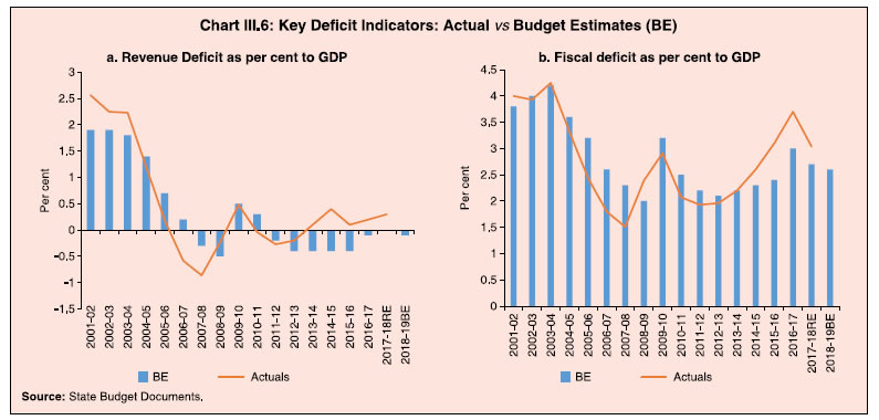

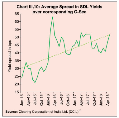
3.34 Acknowledging the centrality of PFM in global best practices, the PEFA (Public Expenditure and Financial Accountability)¹³ programme has developed a framework for assessing and reporting the strengths and weaknesses of PFM using quantitative indicators. It has increasingly been used in the assessment of sub-national government PFM performance¹⁴.

3.35 PEFA includes 31 indicators, grouped under seven pillars, of which budget reliability is the first pillar. It has three indicators (PI-1 to PI-3) assessing the aggregate expenditure, expenditure composition and revenue outturns of state budgets. Each indicator is scored on a four-point ordinal scale: A, B, C or D (A being the best and D the worst). Chart III.8 provides the distribution of the assessment results of the expenditure and revenue outturns of individual state budgets for three years from 2015 to 2017¹⁵. States performed weakly in PEFA scores for PI-1 and PI-3¹⁶. Most states fall in the region of C for expenditure, implying that the aggregate expenditure outturn is between 85 per cent and 115 per cent of the approved budgeted expenditure in at least two of the last three years. In the case of revenue, most states are in the worst zone - D implying aggregate revenue outturn is beyond 92 per cent and 116 per cent of the approved budgeted expenditure in at least two of the last three years. Also, the overall expenditure and revenue outturns are generally less than the approved budgets.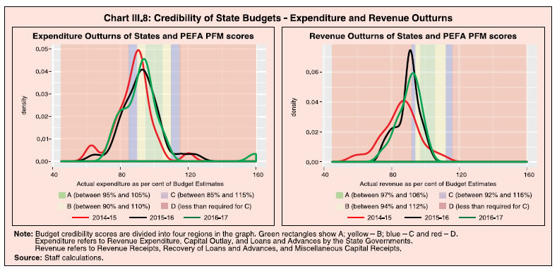

3.36 A snapshot of the individual credibility scores of the 31 state budgets analysed shows that states perform weakly in terms of their budget reliability, with the majority of states remaining in the lowest range i.e., C or D (Table III.4).

6. States’ Market Access

3.37 Another important aspect of fiscal space is the capability of states to access the market without disrupting macroeconomic and financial stability. Following the fourteenth Finance Commission’s recommendation, state governments have reduced their reliance on the National Small Savings Fund (NSSF). Consequently, recourse to market borrowings for funding their fiscal deficits has increased steadily in recent years, particularly during 2013-2017 (Chart III.9). Large issuances of State Development Loans (SDLs), among other factors, have been exerting upward pressure on yields, with the weighted average yield on the state government securities increasing to 7.60 per cent in 2017-18 as against 7.48 per cent witnessed during 2016- 17. The average spread of SDL yields over corresponding maturity central government security (G-sec) yields remained at elevated levels over the last few years (Chart III.10).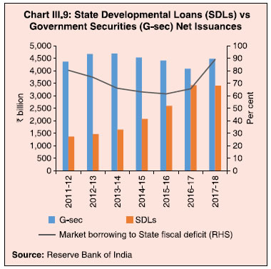

3.38 It has been observed that the fiscal performance of states does not influence much the yield spread on SDLs (Saggar et al, 2017; Bose et al, 2011). The inter-state spread during 2017-18 was only 6 basis points (bps) (7 bps in 2016-17), when the GFD to GSDP ratio ranged between 1.7 and 12.7 per cent in 2017-18 (RE). With markets not differentiating between states in terms of their fiscal deficit or debt positions, recourse to this relatively cheaper source of funding has increased, with little incentive to improve fiscal performance. More recently, however, there is some evidence of market discipline working in determining SDL spreads across states, particularly in 2017-18 (Box III.2).

Box III.2: SDL Yield spreads: Do they Reflect Underlying Fundamentals? Mispricing of sovereign default risk in the years leading up to the global financial crisis and the post-crisis panic in market reactions to fiscal fundamentals has attracted considerable research attention (Sola and Palomba, 2015). State finances and financial markets can get locked into perverse and self-fulfilling interactions. Weak state finances and the consequent higher market borrowings feed into higher yields and spreads, increasing interest payments and debt, worsening state finances further and leading to still higher yields. In reality, however, this vicious circle does not operate for many sub-national governments, including in India, due to institutional circuit breakers like transfers, guarantees and bail outs by the centre (Beck et al, 2017; Schuknecht et al, 2009). For Indian states, fiscal rules based on the fiscal deficit as the target have been in place. The rules were further revised to include debt targets as well as per the revised FRBM adopted in the Union Budget, 2018- 19. While market liquidity indicators like aggregate trading volume or frequency of trading have been observed to be important determinants of cross-state yield spreads (Saggar et al, 2017), the fiscal situation of states represented by the debt to GSDP ratio, particularly when central government faces borrowing constraints in the form of high fiscal deficits, has also been observed to play an important role in influencing positively the spreads in a cross-country framework (Beck et al, 2017). Analysis of state development loans (SDLs) yield spread data for 2017-18 shows some evidence of market disciplining for Indian states. The relationship between the spread on SDLs and the debt outstanding of individual states has marginally improved from no relationship in 2014-15 to weakly positive during 2017-18, albeit at much higher levels of spreads (Chart 1). Using SDL spread over corresponding G-secs as a dependent variable, a panel data model of the form set out below is estimated for 29 states for the period 2006-07 to 2017-18: 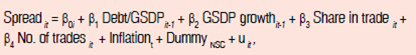where Spreadit is the yield spread of SDL of state i at time t as obtained from CCIL. Among the explanatory variables, apart from the debt to GSDP ratio, control variables include the macro-economic situation of states proxied by lagged GSDP growth; liquidity of the SDL bond as measured by (a) ratio of the traded value of the particular SDL to the sum of all traded values of all SDLs issued by all states in that year, and (b) number of trades in that particular SDL. Both GSDP growth and liquidity variables are likely to be negatively associated with yield spread. Inflation is used as a proxy for the overall macro-economic situation. A state-specific dummy (DummyNSC), based on whether a state is in the non-special category (NSC) or not, and a time dummy, based on whether the centre has seen a slippage in that year or not have also been introduced in alternate versions of the model in line with the literature. The results are given in Table 1. The results indicate that states’ fiscal matrix, proxied by lagged debt to GSDP ratio, has a positive sign but is not significant for the full period 2006-07 to 2017-18 and turns out to be significant only in a cross-section framework for 2017-18 (third column). Liquidity of SDLs as represented by share in trades seems to be important for the post-crisis period in explaining variations in spreads. Lagged GSDP growth is also significant and shows the expected negative sign. Among common factors across states, inflation is positive and significant, implying that deteriorating macro fundamental affects significantly the yield spreads irrespective of state-specific factors. When the above exercise is repeated for years when the centre has seen a slippage, the significance of β1 improves (last two columns of Table 1) indicating that any slippage by the centre makes markets conscious of the weak federal fiscal position and, in turn, affects its capacity to support states. Accordingly, the market players behave more responsibly and put higher risk premia for fiscally weaker sub-sovereigns. This result is similar to that of Beck et al. (2017) who show that higher sub-sovereign debt levels are scrutinised more by financial markets if federal sovereign risk is high. Going forward, it is important that fiscal discipline becomes an inherent part of states, both explicitly via operation of fiscal rules and implicitly via markets through the risk-sensitive premia. Table 1: SDL Yield spread and States’ debt outstanding: Panel Data Estimation   Full period (2006 -07 to 2017-18) Post crisis (2009-10 to 2017-18) 2017-18 Full period (2006-07 to 2017-18) Post crisis (2009-10 to 2017-18) Debt/GSDP 0.100 0.601 0.159**     (1.65) (1.33) (1.96)     Debt/GSDP (For years when Centre dummy takes value 1)       0.193*** 0.476***       (3.19) (5.28) Share in trade 0.0678 -0.937*** 0.361 0.350 -0.187 (0.20) (-3.13) (1.04) (1.05) (-0.50) Log Trades (in number) -0.794 3.013* -0.0725 -1.735** -0.142 (-0.96) (1.94) (-0.07) (-2.12) (-0.15) Lagged GSDP growth -0.235** -0.286*** 0.408* -0.198* -0.293*** (-2.09) (-3.20) (1.86) (-1.81) (-2.67) Inflation in % 2.030*** 2.721*** 0 1.518*** 3.149*** (5.25) (-2.02)   (3.64) (4.88) DummyNSC 2.697 -4.918** -0.959 3.851 -2.022 (0.98) (-2.02) (-0.33) (1.40) (-0.66) Constant 32.32*** 17.14*** 36.65*** 39.98*** 17.93*** (5.87) (3.61) (5.77) (8.45) (2.77) N 296 244 28 140 112 t statistics in parentheses * p < 0.1, ** p < 0.05, *** p < 0.01 References: Beck, R., Ferrucci, G., Hantzsche, A., & Rau-Goehring, M. (2017). Determinants of sub-sovereign bond yield spreads–The role of fiscal fundamentals and federal bailout expectations. Journal of International Money and Finance, 79, 72-98. Saggar S, Rahul T and M Adki (2017), “State Government Yield Spreads – Do fiscal metrics matter?” MSM, RBI, 08. Schuknecht, L., Von Hagen, J., & Wolswijk, G. (2009). Government risk premiums in the bond market: EMU and Canada. European Journal of Political Economy, 25(3), 371-384. Sola, S., & Palomba, G. (2015). Sub-National Government’s Risk Premia: Does Fiscal Performance Matter? IMF Working Paper, WP 15/117.

3.39 On the demand side, the demand for SDLs from commercial banks emanates from regulatory prescriptions – Statutory Liquidity Ratio (SLR); Liquidity Coverage Ratio (LCR) and normal investment demands¹⁸. Banks’ investments in SDLs have risen from 16 per cent of total government securities in early 2000s to about 24 per cent during 2017 (Chart III.11). Within the total holding, there are notable bank group-wise variations. While the share of public sector banks is higher at above 30 per cent of total government securities, it is about 10 per cent for private banks and almost negligible for foreign banks.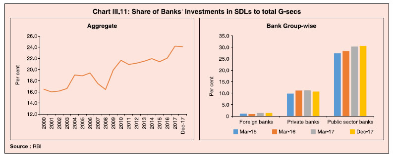

3.40 While the supply and demand for SDL issuances remains high, the secondary market liquidity of SDLs is low. Daily average turnover of SDLs in the secondary market is about one-tenth of that for central government securities. Looking at the turnover ratio measured as SDL traded volume scaled by outstanding stocks, it is observed that SDL liquidity is very low vis-à-vis central government securities (Chart III.12).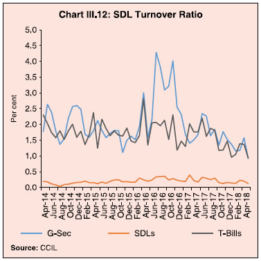

3.41 The RBI has sought to enhance the liquidity of SDLs by shifting to weekly auctions from fortnightly auctions so that issuance sizes are smaller and evened out. The release of high frequency state finances data is expected to enable detailed analysis and comparison (RBI, October 2017)¹⁹. In order to address near to medium term redemption pressures on states arising out of outstanding SDLs maturing (as discussed in Chapter II), and also to further incentivise state governments to increase the corpus of Consolidated Sinking Fund (CSF) and the Guarantee Redemption Funds (GRF)²⁰, the RBI has lowered the rate of interest from 100 bps to 200 bps below the Repo Rate on the Special Drawing Facility (SDF) from the Reserve Bank against the collateral of the funds in CSF and GRF (RBI, June 2018). Remaining few states are encouraged to become member of these funds so as to have buffers for repayment of their liabilities as also avail SDF to bridge the cash-flow mismatches which is in addition to Ways and Means advances (WMA).

3.42 With the objective of promoting differential and market-based pricing, the process of valuation of SDLs in banks’ portfolios has been altered from a uniform mark up of 25 basis points above the centre’s G-sec yield to differential valuation based on prices at which they are traded in the market or at primary auctions. While harmonising the Liquidity Adjustment Facility (LAF) haircuts with international standards, the initial margin requirement for rated SDLs has been set at 1.0 per cent lower than that of other SDLs for the same maturity buckets, primarily with the objective of encouraging state governments to get a public rating on their SDLs (RBI, June, 2018). Going forward, SDL yields should reflect more sensitively the risk asymmetries across states, enabling fiscally sound states to borrow at a cheaper rate and nudging other states to try and reduce their fiscal deficits and debt.

7. Concluding Observations

3.43 There are visible signs of fiscal pressures emerging in several states, particularly due to expenditure schemes that have been detailed in this Chapter. These schemes could be made more productive by closing ‘efficiency gaps’; better targeting/ reducing leakages; and careful planning as well as better forecasting so that outgoings from the state budgets are financed through revenue resources and transfers.

3.44 On the revenue front, the GST implementation could pave the way for generating higher revenues through greater efficiency and broadened tax base. States have, however, increased reliance on market borrowings to meet expenditures given the recurring shortfall in revenue receipts relative to budgeted targets. Market borrowings provide easy access to finance for states, but the present lack of incentives to undertake fiscal reform so as to earn lower spreads could render state finances vulnerable to debt sustainability concerns. Steadily rising yields on SDLs imply the need for larger and faster corrections in primary deficits than before so as to adhere to the revised FRBM target of 20 per cent for the state-level debt to GDP ratios by 2024-25. However, attaining this in a scenario of large committed expenditure could lead to compromise on the developmental and capital expenditure, which may not be desirable from a long-term growth perspective. Hence, re-prioritising state expenditures and improving their efficiency will be necessary to sustain growth while maintaining fiscal prudence.

¹ FC-XIII had recommended that states should follow a recruitment and wage policy, in a manner that the total salary bill relative to revenue expenditure (net of interest payments and pensions) does not exceed 35 per cent.

² As per data on wages and salaries provided by state governments that implemented pay commission awards in 2017-18. These data do not include pensions.

³ The benefits of the debt waiver in these states were given to the farmers in the year of implementation but the reimbursements to the lending institutions by the state governments is being done in a phased manner, over a five year period for Andhra Pradesh and Tamil Nadu. Telangana has completed its reimbursement by 2017-18.

⁴ In 2017, Karnataka had announced farm debt waiver of ₹82 billion.

⁵ With a view to encouraging credit discipline, the Tamil Nadu Government has, since 2009-10, been providing full interest relief to farmers for prompt repayment of crop loans taken from co-operatives.

⁶ Under Antyodaya Anna Yojana (AAY), each household continues to get 35 kg of foodgrains per month.

⁷ Additional food grains are provided under tide over allocation at a higher CIP of ₹8.30 and ₹6.10 for rice and wheat, respectively.

⁸ Uttar Pradesh which was earlier under the DCP scheme opted out in 2012.

⁹ CAG, 2015, Audit of the Preparedness for Implementation of National Food Security Act, 2013 for the year ended March 2015, Comptroller and Auditor General of India Report No.54.

¹⁰ Action taken includes suspension or cancellation of licences/show cause notices issued/first information reports (FIRs) filed.

¹¹ Saini et al, 2017, Indian food and welfare schemes : Scope for digitization of cash transfers, Working Paper 343, Indian Council for Research on International Economic Relations, August.

¹² Fiscal marksmanship refers to the accuracy of budgetary forecasting and checks for the budget missing its own targets. It indicates how efficiently government uses all available information for budgetary procedures.

¹³ PEFA is a methodology for assessing public financial management performance. It identifies 94 characteristics (dimensions) across 31 key components of public financial management (indicators) in 7 broad areas of activity (pillars). PEFA programme was initiated in 2001 by seven international development partners: the International Monetary Fund, the World Bank, the European Commission and the governments of France, Norway, Switzerland and the United Kingdom. For details on methodology refer to PEFA Framework for assessing public financial management (PEFA Secretariat 2016).

¹⁴ World Bank (2009.) India-Himachal Pradesh Public Financial Management Accountability Assessment. Financial Management Unit, South Asia Region, World Bank, June.

¹⁵ The assessment is restricted to the period for which accounts data were available at the time of the exercise.

¹⁶ PI-1 (Aggregate expenditure outturn) measures the extent to which the aggregate expenditure outturn reflects the amount originally approved in the budget (Budget Estimates). Based on the methodology provided by the PEFA programme, a score of A is given for PI-1 if the aggregate expenditure outturn is between 95 per cent and 105 per cent of the approved budgeted expenditure in at least two of the last three years. Similarly PI-3 (Revenue outturn) measures the change in revenue between the original approved budget and actual outturn. A score of A is given for PI-3 if the actual revenue is between 97 per cent and 106 per cent of budgeted revenue in at least two of the last three years (the minimum requirements for other scores i.e. B, C and D can be inferred from the charts).

¹⁷ This spread is calculated for outright deals of ₹5 crore and above settled through CCIL and SDL spreads are over corresponding maturity G-secs.

¹⁸ The decline in SLR from 25 to current 19.5 per cent has been suitably calibrated to adjust for the periodic rise in LCR to reach 100 per cent by January 1, 2019.

¹⁹ The attempt to release data for two state budgets 2017-18 and 2018-19 in this issue of the State Finance Report, so as to eliminate the lag in the publication of the data is also a small step in this direction.

²⁰ State governments are maintaining the Consolidated Sinking Fund (CSF) and the Guarantee Redemption Funds (GRF) with the Reserve Bank as buffers for repayment of their liabilities. Currently, state governments can avail of Special Drawing Facility (SDF) from the Reserve Bank against the collateral of the funds in CSF and GRF.