by Satyananda Sahoo, Kunal Priyadarshi, Chaitali Bhowmick, Sapna Goel and Preetika^ Economic activity in the Indian states is impacted by national and state-level policies as well as global developments. Output is thus subject to both common and idiosyncratic shocks. Synchronisation of national and sub-national cycles is probed through trend-cycle decomposition of regional gross state domestic product using alternate filters. A more disaggregated analysis of factors driving the synchronsiation follows using correlations from state-level cycles. The study finds stronger co-movement of western and southern regions with the national cycle since the 2000s and larger bearing of common components on the regional cycles. The study also underscores the positive role of geographical proximity on synchronisation of business cycles. Introduction The Indian economy functions under a well-established federal structure in which states are governed by both centralised policies (for example, monetary policy, fiscal policy, external trade policy), as well as state-specific policies adopted by individual state governments. Indian states exhibit distinct macroeconomic and social structures reflected in widely varied sectoral compositions, inflation dynamics, physical and social infrastructure, the level of financial literacy and so on. Reflecting these dynamics, states are subject to common and idiosyncratic shocks. The complex amalgamation of all these factors warrants a probe into how synchronised state-level economic aggregates are vis-à-vis the national gross domestic product (GDP) cycle, and how the common and state-specific factors and spillover effects across states play around in determining the overall macro dynamics of Indian states. Most of the research on growth dynamics of Indian states has focused on growth convergence or divergence, overlooking the dynamics of business cycles altogether. Much of the empirical work on business cycles at state or regional level exists in the context of the United States (US), Australia and the European Union (EU). The analysis of business cycles at sub-national level in emerging market economies (EMEs) is scant primarily due to non-availability of long time series data on the relevant macro aggregates. In view of the above, this paper aims to fill this gap by exploring the growth dynamics and the nature of co-movement of business cycles of Indian states over the past four decades. The paper also attempts to understand the extent to which fluctuations in state economic activity are driven by common factors impacting all states in unison and idiosyncratic shocks which may include an event of drought or any other natural calamity in some state, or state-specific fiscal or regulatory measures. The spillover of shocks across states is examined in terms of dynamic cross-correlation of state business cycles. The period of study spans from 1980-81 to 2019-20 based on availability of common data set and excluding COVID-19 pandemic aberrations. The Baxter-King’s (B-K) band-pass filter and Kalman filter under the unobserved component model (UCM) framework are used for trend-cyclical decomposition of the states. Synchronisation of national and sub-national cycles is examined by aggregating major Indian states and union territories (UTs) into five regional groups according to their geographical settings for brevity. Furthermore, factors underlying the dynamics of business cycle synchronisation have been explored at a more disaggregated level using state-level cycles. In particular, the study attempted to explore whether geographical location and the economic structure of the states matter to the dynamics of synchronisation of cycles using ordinary least squares (OLS) regression. States with similar economic structures might get impacted by similar type of shocks which may result in co-movement in their cycles. On the other hand, forward and backward linkages and sectoral spillovers across states could be strong enough to influence cycles of states with differing economic structures but sharing complementarities. Therefore, how economic structure of a state plays a role in shaping its business cycle appears equivocal and, warrants an empirical exploration. The study finds evidence of increasingly higher synchronisation of cycles post 2000 for the western and southern regions with the national business cycle and larger bearing of common components on regional cycles. In contrast, for the northern, eastern and central regions, the degree of synchronisation with national cycle has weakened, which might be, inter alia, reflective of the prevalence of idiosyncratic shocks and/or growing divergence in sectoral compositions of these regions vis-à-vis the national level. Moreover, both regional and state-level analysis highlighted substantial impact of geographical proximity of states on business cycle synchronisation. Set against this backdrop, the paper is organised in six sections. Section II underscores the major stylised facts regarding growth dynamics of Indian states over the last four decades. Section III discusses the relevant literature followed by data description and methodology in section IV. Section V presents the major findings from the analysis. Section VI concludes the paper. II. Stylised Facts Gross state domestic product (GSDP) of twenty states and four UTs1, accounting for more than 95.0 per cent of India’s real GDP has been considered for the analysis, the data for which are sourced from the National Statistical Office (NSO). For succinctness, the select states, based on their geographical locations, are aggregated into five different regions based on the Zonal Councils of India (Table 1 and Chart 1). North eastern region has not been included due to unavailability of longer time series of select north-eastern states viz., Mizoram, Nagaland and Sikkim. In sync with India’ growth story, the compound annual growth rates (CAGR) across regions accelerated markedly during 2000s. The western region, comprising Goa, Gujarat and Maharashtra, outperformed other regions between the 1980s and 2010s, the CAGR in the southern region surpassed the western states in the last decade (2010-11 to 2019-20). In level terms, GSDP at constant prices of the southern region exceeds that of the western region by 27.6 per cent in 2019-20 (Table 2). | Table 1: Regional Classification of Indian States and Union Territories | | Northern | Western | Eastern | Southern | Central | | Chandigarh | Goa | Bihar | Andhra Pradesh | Chhattisgarh | | Delhi | Gujarat | Jharkhand | Karnataka | Madhya Pradesh | | Haryana | Maharashtra | Odisha | Kerala | Uttarakhand | | Himachal Pradesh | | West Bengal | Puducherry | Uttar Pradesh | | Jammu and Kashmir | | | Tamil Nadu | | | Punjab | | | Telangana | | | Rajasthan | | | | | | Source: Zonal Councils of India. |
 An overview of economic activity composition exhibits that in the last decade, services have been contributing more than 50.0 per cent to gross state value added (GSVA) on average in all regions. While services comprise on average 65.4 per cent of the activity in the southern region, central region has the lowest share at 53.6 per cent. In comparison to other zones and national level, the western region has the largest proportion (roughly one-third of the region’s economy) contributed by industry; in Gujarat the average share of industry is closer to twice of the national level. Both central and eastern regions have on an average 20 per cent share of agriculture and allied activities in their GSVA [Chart 2]. Amongst all, the northern region, closely mirrors the national sectoral structure. 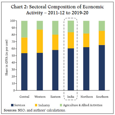 Delving further into the states in the respective regions, Rajasthan has the maximum share in northern region GSDP followed by the NCT of Delhi; Maharashtra has the largest share in GSDP of the western region followed by Gujarat; in the eastern region, West Bengal is followed by Bihar and Odisha; Tamil Nadu and Karnataka hold a major share in the southern region. In the central region, Uttar Pradesh holds more than half of the region’s GSDP share. Differences in growth across states have widened disparities in some regions, while in others, growth has remained largely synchronised (Chart 3). The differences in the economic structures across states and regions can, inter alia, contribute to growth variations (Chart 4). | Table 2: CAGR of Real GSDP (in per cent) – Region-wise | | | Northern | Western | Eastern | Southern | Central | India | | 1981-82 to 1989-90 | 5.4 | 6.0 | 4.4 | 5.3 | 4.7 | 5.6 | | 1990-91 to 1999-2000 | 5.4 | 6.7 | 4.7 | 5.9 | 4.1 | 5.7 | | 2000-01 to 2009-10 | 7.1 | 7.8 | 6.4 | 7.1 | 6.3 | 6.3 | | 2010-11 to 2019-20 | 6.7 | 7.2 | 6.0 | 7.3 | 6.5 | 6.6 | | Sources: NSO; and authors’ calculations. |
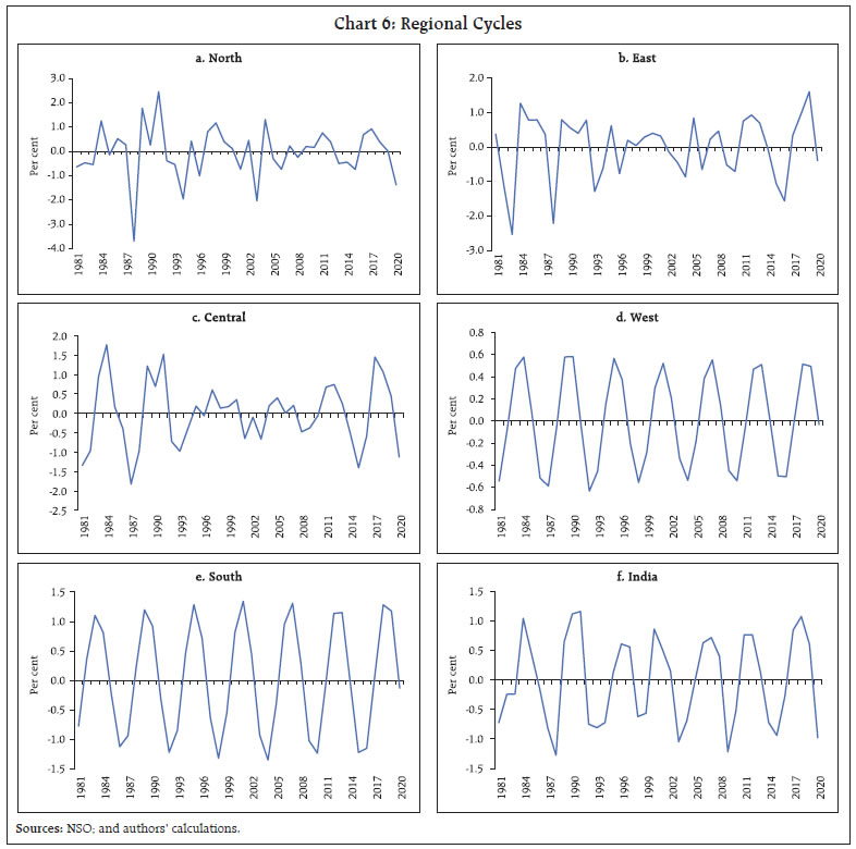
III. Literature Review Business cycles are the outcome of movements in multitude of economic variables interacting with each other. Research on business cycles has an extensive history concerning both theory and empirical work. Classical techniques of business cycle analysis dates to the pioneering work by researchers at the National Bureau of Economic Research (NBER) [Mitchell (1927); Mitchell and Burns (1938); and Burns and Mitchell (1946)]. Empirical research related to business cycles primarily centres on two key questions – first, how to identify and distinguish alternative phases i.e., the peaks and troughs of the business cycle and identify the turning points? and, second, how to explain the observed co-movement of specific time series with the aggregate business cycle? Kaldor’s (1957) focus on stylised facts of growth in terms of long-term trend movement of an economy and later Lucas’s (1976) stylised facts of movements about trends in gross national product led the foundation of long traditions of research on business cycles in context of advanced economies (AEs). 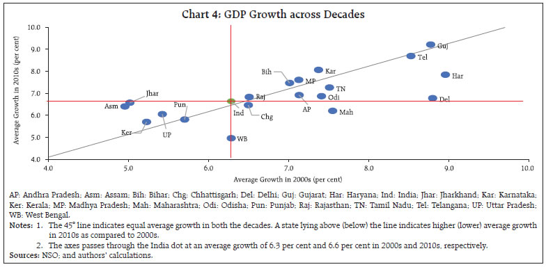 Much of the empirical work on business cycles has focused on the US, Australia, the EU and the African region. Magrini et al. (2013), using data for 48 co-terminus US states between 1990 and 2009, analysed the degree of synchronisation by means of trade openness, financial integration and industrial specialisation along with their interlinkages, and found a possible circular relationship between the degree of synchronisation and a general index of sectoral specialisation. Kouparitsas (2002) found that while spillovers of region-specific shocks account for a not statistically significant share of business cycle variation of regional per capita income, common shocks have a large and statistically significant share. A study on regional business cycles of Australia too finds the enormous effect of common components such as fluctuations in world demand or terms of trade on co-movement of state business cycles as compared to state-specific or idiosyncratic shocks (Norman and Walker, 2007). Agénor et al. (2000) explored the main stylised features of macroeconomic fluctuations for twelve developing countries based on cross-correlations between domestic industrial output and various macroeconomic variables such as wages, inflation, money, credit and exchange rates. A study based on a larger sample of thirty-two developing countries finds that output, consumption, investment, government revenue and expenditure of developing countries were more volatile and less persistent in comparison to developed countries whereas real interest rates were less volatile (Male, 2010). Although India is included as one of the countries in the sample, such studies do not show the changing nature of business cycle of any specific country over time. Ghate et al. (2013) focused exclusively on Indian data to study the properties of Indian business cycle over two periods – pre and post liberalisation. The findings suggest that properties of the cycle had moved closer to AEs mainly due to the transition of the economy from agricultural to a market based industrial economy post liberalisation. Extensive work exists on measurement, dating and drivers of the Indian business cycle (Pandey et al., 2016, 2018). Both these studies focus on the chronology of the Indian business cycle in the post-reform period and observed that the average duration of expansion is estimated to be around twelve quarters while that of recession is around nine quarters with amplitude of recession being higher than that of expansion. In the aftermath of 2008 global financial crisis, economic cycles in the Indian states displayed stronger co-movement with the national cycle and growth cycles have been more pronounced in non-agricultural states relative to agricultural states (Ahmad et al., 2018). Majority of the work on Indian states focused on convergence or divergence in the growth rates, overlooking the business cycles altogether. Ahmad et al. (2018), while touching upon growth cycles at state-level, do not delve into detailed dynamics of the observed trends. IV. Data and Methodology One of the prerequisites of any robust macroeconomic analysis is the availability of consistent time series of macroeconomic variables of suitable length. Our study involves a period spanning 1980-81 to 2019-20. Prime motive for choosing such a time period is the availability of a common dataset for all states considered. The period prior to the 1980s is not considered as it was marked by a series of domestic (such as drought) and external shocks (e.g. oil price spikes) which prevented the interplay of investment-inventory fluctuations that creates business cycles (Pandey et al., 2018). Moreover, GSDP data are subject to multiple base revisions, and during the period of our study, GSDP data are available at five different base years namely, 1980-81, 1993-94, 1999-2000, 2004-05 and 2011-12. Therefore, GSDP series at a single base year 2011-12 has been generated for the entire period using the standard splicing method.2 During the period of study, four states were bifurcated – Uttarakhand, Jharkhand and Chhattisgarh from Uttar Pradesh, Bihar and Madhya Pradesh, respectively, in 2000 and Telangana from Andhra Pradesh in 2014. Hence, to generate the series where data are not available, the growth rate of the combined state has been assumed for both the bifurcated states. Further, to avoid pandemic induced aberrations which disrupted the usual trend-cycle properties, post-COVID years are excluded. Following the standard business cycle literature, this study emphasises on growth cycle,3 as India being a high growing economy, the evidence of classical cycles are non-existent and the same holds true at the state-level. Among available filtering techniques for trend-cycle decomposition from GSDP data, the B-K band-pass filter which introduces less distortion compared with other popular filters viz., the Hodrick-Prescott (HP) filter has been used to decompose the trend and cyclical components of the regions/states. Furthermore, we have also followed the unobserved component (UCM) approach for the trend-cycle decomposition of regional economic fluctuations. Following Watson (1986) and other business cycle literature, this study assumes that logarithm of GSDP for region i at time t denoted by yit comprises a trend and a cyclical component (Equation 1); the trend of yit has a random walk with drift where the drift term is denoted by δit (Equation 2); and the cyclical component is a stationary second-order autoregression process (Equation 3). μit is the random error component of region i’s GSDP at time t. 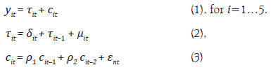 The synchronisation of business cycles is studied by juxtaposing the regional cycles against the national GDP cycle. The observations from visual representation of cycles are further corroborated by correlation analysis. The dynamics of synchronisation of cycles have been evaluated through rolling window correlations between the national and regional cycles. Given the annual frequency of data, the window length has been set at ten years which is a period sufficient to capture a complete full-length business cycle – from peak-to-peak or trough-to-trough. Furthermore, examining deeper into the nature of synchronisation, observed co-movement of cycles could be either due to some common factors such as policy changes at the national level which affect all regions simultaneously, or spillover of idiosyncratic shocks across regions. The hypothesis whether geographical proximity and sectoral composition of constituent states leads to stronger transmission of regional shocks has been studied by comparing cross-correlations across regions. In case of spillovers, any event in a particular region will influence the business cycle of that region with immediate effect but will gradually transmit to other regions through various economic transactions or sentiments and impact cycles of other regions with a lag. Therefore, the spillover effect could be gauged by lead-lag correlations of cycles across region. In our study, the spillover effect is examined by one-year lag cross-correlation of cycles across regions assuming that one year period is adequate enough for transmission of idiosyncratic shocks from one region to the other. Finally, state-level analysis is carried out to explore how varied shocks and their spillover effects impact business cycle synchronisation. Two hypotheses have been tested in an OLS regression framework in this regard. Hypothesis I: Geographical proximity strengthens co-movement of business cycles. Hypothesis II: Economic structure of states influences business cycles synchronisation through sectoral linkages and complementarities. Pair-wise correlation coefficients of states have been considered as dependent variable for the stated hypotheses. With a total of twenty states and four UTs, 276 observations of pair-wise correlations have been found. Geographical proximity is defined by whether two states share at least one common geographical border and is included in the model as a dummy variable which assumes a value one if the states share borders and, zero otherwise. The economic structure of a state is defined in terms of the sector contributing the highest to the state’s GSVA vis-à-vis the share of that sector at the national level. For instance, a state is termed as an agricultural state if the difference between the share of agriculture in state’s GSVA and national share of agriculture in GVA is the highest when compared with the same for industry and services sector. The dummy variable relating to economic structure used in the model assumes a value one if two states share similar structure (say, both being agricultural states), and zero otherwise. Additionally, an interaction of the two dummies has been added as a variable to gauge the impact on synchronisation. V. Findings Regional business cycles derived from both B-K filter and UCM show moderate synchronisation with the national cycle and cyclical fluctuations tend to diminish over time as reflected in slightly lower amplitudes of cycles over the later period (Charts 5a and 5b). As cycles derived from the B-K filter and UCM display similar movement, the rest of the analysis is based on cycles generated from the UCM approach. Cyclicality is more pronounced in case of western and southern regions in comparison with other regions. These two regions also appeared as the major drivers of the national GDP cycle, probably, because the nine major states and UTs comprising western and southern regions considered in this study account for more than half of the national GDP. Central region with leading share of agriculture in overall GSVA also depicts relatively higher co-movement (Chart 6). The observed patterns of cyclicality from the visual representation have been reinforced by the correlation analysis (Table 3). All regions present high and statistically significant correlation with the national cycle as well as high cross-correlation across regions, except a few. For the overall period, central region portrays the highest correlation with the national cycle followed by western and southern regions. Cross-correlations indicate that geographical proximity and sectoral composition of the constituent states have an influence over synchronisation of regional cycles. The northern region with relatively lower share of industrial activity and in relatively closer proximity with eastern and central regions exhibited a higher cross-correlation among them. Similarly, many of the states belonging to the western and southern regions share their borders and are more industrialised compared to other regions which might explain higher cross-correlation between these two regions. The not statistically significant correlation between the northern and the southern regions could be reflecting the innate structural and compositional differences across them. The degree of synchronisation over time has been evaluated in terms of rolling window correlations between cycles of each region with the national cycle. The correlation coefficients computed for each of the 10-year rolling window starting from 1981-82 are placed against the last year of the window (Chart 7). The synchronisation of cycles appears to be largely governed by the income levels, as in the initial years till the mid-2000s, the relatively richer northern states dominated the overall cyclical movement. In the subsequent period, the western and southern regions, by virtue of fast-paced growth, gradually surpassed the northern and central regions to gain larger influence over the national cycle. Post 2014, however, the northern region has caught up with the two regions quite well. For the overall period, the central, western and southern regions exhibited higher synchronisation4 with the national cycle (Chart 8). 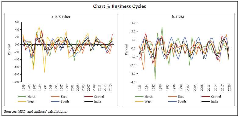
| Table 3: Cross-Correlation across Regions | | | Northern | Eastern | Central | Western | Southern | India | | Northern | 1.00 | | | | | | | Eastern | 0.47*** | 1.00 | | | | | | Central | 0.60*** | 0.39** | 1.00 | | | | | Western | 0.02 | 0.28* | 0.55*** | 1.00 | | | | Southern | -0.06 | 0.24 | 0.45*** | 0.98*** | 1.00 | | | India | 0.51*** | 0.55*** | 0.75*** | 0.70*** | 0.64*** | 1.00 | Note: ***, ** and * indicate statistical significance at 1 per cent, 5 per cent and 10 per cent, respectively.
Sources: NSO; and authors’ calculations. | 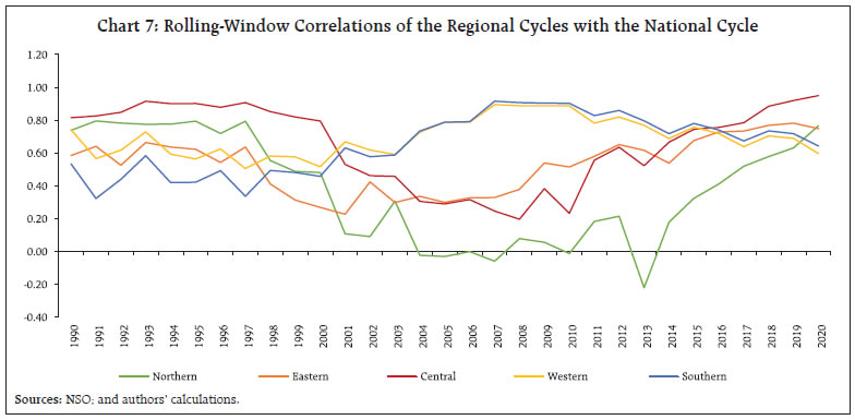 To explain the co-movement of cycles, the framework followed in Norman and Walker (2007) has been adopted which interprets the observed cyclical co-movement as a result of either common shocks, spillovers of idiosyncratic shocks, or a combination of the two (described in section IV). A higher correlation between activity in one region with lagged activity in another as compared with their contemporaneous correlations would suggest that spillovers are more important than common shocks. Majority of contemporaneous correlations (Table 3), however, turn out to be higher than lagged correlations (Table 4) for all regions suggesting a higher influence of common components such as national policies, domestic shocks like deficient rains/adverse climate events, or shocks to global variables etc. The central and southern regions displayed significant lagged correlation with other regions. In particular, the central region had the highest one-year lagged correlation with the eastern region. Higher spillover from the central region might reflect the impact of climate-related disruptions such as Uttarakhand floods of 2013, droughts and heatwaves in Uttar Pradesh, Madhya Pradesh and Chhattisgarh during 2002, 2009 and 2015-16, affecting the agriculture-intensive states of central region and gradually spilling over to other regions. 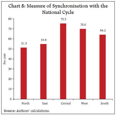
| Table 4: One-year Lagged Correlations | | | Northern | Eastern | Central | Western | Southern | India | | Northern lagged | -0.23 | -0.30* | 0.23 | 0.11 | 0.02 | 0.08 | | Eastern lagged | 0.23 | 0.03 | 0.72*** | 0.37** | 0.29* | 0.47*** | | Central lagged | -0.07 | -0.47*** | 0.32** | 0.20 | 0.19 | 0.11 | | Western lagged | -0.16 | -0.11 | 0.25 | 0.46*** | 0.57*** | 0.23 | | Southern lagged | -0.15 | -0.07 | 0.17 | 0.34** | 0.47*** | 0.19 | | India lagged | 0.03 | -0.17 | 0.45*** | 0.37** | 0.35** | 0.32** | Note: ***, ** and * indicate statistical significance at 1 per cent, 5 per cent and 10 per cent, respectively.
Sources: NSO; and authors’ calculations. | Having analysed the regional cycles, further insights regarding the factors shaping these cyclical movements have been drawn using state-level data focusing, particularly, on two aspects – geographical location and economic structure of the states. As already expounded, the economic structure of a state is based on the sector contributing the highest share in its GSVA relative to the share of that sector in the national GVA. If sector-specific shocks are prominent, they are likely to reflect in higher co-movement of cycles of structurally similar states. On the other hand, strong inter-sectoral linkage would reflect in better synchronisation of business cycles of states with different sectoral orientations. The cross-correlation matrices of state business cycles for all possible combinations of economic structure have been used to explore these factors. Among the cohorts with similar sectoral orientation, business cycles appear to be stronger among agricultural states as compared to the industrial and services-oriented states (Tables 5a, 5b and, 5c). This could be due to the agricultural sector being relatively more prone to climate related disruptions such as droughts, excess or erratic rainfall which impact farming activity. Geographical location of the states does not seem to have any impact on co-movement of cycles in agricultural states. Uttar Pradesh, one of the leading farming states in India displayed significantly strong business cycle correlation with states such as Andhra Pradesh, Rajasthan, Madhya Pradesh and Haryana. In services-oriented states, the geographical proximity might be crucial as the correlation of cycles is significantly high among services-oriented states like Karnataka, Tamil Nadu, Kerala and Telangana. The synchronisation of cycles between the agriculture-industry pair and agri-services pair is significantly high for several states – both neighbouring as well as far-way states (Tables 6a and 6b). This could be due to national level policies including price controls and subsidies, or diffusion of technology and infrastructure development resulting in better economic ties across agricultural and services states. Maharashtra, a major industrial state, also depicted strong correlations with the services oriented southern states (Table 6c). | Table 5: Cross-Correlation across Similar Sectoral Orientation | | a. Agriculture | | Agriculture | Har | Pun | Raj | WB | UP | MP | AP | | Har | 1 | | | | | | | | Pun | -0.17 | 1 | | | | | | | Raj | 0.35** | -0.10 | 1 | | | | | | WB | 0.15 | -0.12 | 0.13 | 1 | | | | | UP | 0.37** | 0.02 | 0.43*** | 0.31* | 1 | | | | MP | 0.23 | 0.11 | 0.41*** | 0.09 | 0.31** | 1 | | | AP | 0.26 | 0.40** | 0.22 | -0.21 | 0.66*** | 0.27* | 1 | | b. Industry | | Industry | HP | Jhar | Odi | Chg | UK | Goa | Guj | Mah | Pudu | | HP | 1 | | | | | | | | | | Jhar | 0.05 | 1 | | | | | | | | | Odi | 0.51*** | 0.03 | 1 | | | | | | | | Chg | 0.31* | 0.01 | 0.34** | 1 | | | | | | | UK | 0.12 | 0.18 | 0.01 | -0.16 | 1 | | | | | | Goa | 0.04 | 0.10 | -0.00 | 0.19 | 0.12 | 1 | | | | | Guj | 0.42*** | 0.27* | 0.32** | 0.01 | 0.30* | 0.11 | 1 | | | | Mah | 0.45*** | -0.22 | 0.25 | 0.45*** | 0.04 | 0.04 | 0.05 | 1 | | | Pudu | -0.39** | 0.18 | -0.20 | -0.33** | -0.14 | 0.16 | -0.11 | -0.94*** | 1 | | c. Services | | Services | J&K | Cha | Del | Bih | Kar | Ker | TN | Tel | | J&K | 1.00 | | | | | | | | | Cha | 0.09 | 1 | | | | | | | | Del | 0.04 | 0.91*** | 1 | | | | | | | Bih | 0.27* | -0.03 | 0.03 | 1 | | | | | | Kar | -0.02 | -0.84*** | -0.70*** | 0.09 | 1 | | | | | Ker | 0.22 | -0.40** | -0.56*** | -0.26 | 0.22 | 1 | | | | TN | 0.25 | -0.73*** | -0.78*** | 0.14 | 0.58*** | 0.52*** | 1 | | | Tel | 0.04 | -0.77*** | -0.60*** | 0.15 | 0.75*** | 0.23 | 0.54*** | 1 | Note: (i) AP: Andhra Pradesh; Bih: Bihar; Cha: Chandigarh; Chg: Chhattisgarh; Del: Delhi; Guj: Gujarat; Har: Haryana; J&K: Jammu and Kashmir; Jhar: Jharkhand; Kar: Karnataka; Ker: Kerala; MP: Madhya Pradesh; Mah: Maharashtra; Odi: Odisha; Pudu: Puducherry; Pun: Punjab; Raj: Rajasthan; TN: Tamil Nadu; Tel: Telangana; UK: Uttarakhand; UP: Uttar Pradesh; WB: West Bengal.
(ii) ***, ** and * indicate statistical significance at 1 per cent, 5 per cent and 10 per cent, respectively.
Source: Authors’ calculations. |
The role played by geographical location and economic structure in synchronisation of state business cycles has been further probed through OLS regression analysis. Pair-wise correlation of state cycles is taken as the dependent variable while dummy variables related to state borders and economic structure as defined previously, along with their interaction constitute the explanatory variables used to test the relevant hypotheses. To ensure robustness and consistency of results, three regressions covering alternative time periods have been specified in order – 1980-2020, 1980-2010 and latest 1991-2020 period with an overlapping period (1991-2010) in the latter two (Table 7). | Table 6: Inter-Sectoral Cross Correlations | | a. Agriculture | | Industry | Har | Pun | Raj | WB | UP | MP | AP | | HP | 0.36*** | 0.45*** | 0.36** | -0.12 | 0.10 | 0.18 | 0.36** | | Jhar | 0.25 | -0.24 | 0.25 | 0.21 | 0.10 | -0.02 | 0.03 | | Odi | 0.20 | 0.26 | 0.31* | 0.20 | 0.12 | 0.11 | 0.24 | | Chg | -0.04 | 0.45*** | 0.17 | 0.03 | -0.06 | 0.57*** | 0.10 | | UK | 0.45*** | -0.01 | 0.29* | 0.13 | 0.75*** | 0.08 | 0.54** | | Goa | 0.14 | 0.04 | 0.28* | 0.33** | 0.45*** | 0.30* | 0.21 | | Guj | 0.30* | 0.02 | 0.70*** | 0.05 | 0.29* | 0.20 | 0.18 | | Mah | -0.16 | 0.99*** | -0.09 | -0.13 | 0.08 | 0.12 | 0.44*** | | Pudu | 0.13 | -0.92*** | 0.07 | 0.18 | -0.12 | -0.06 | -0.50*** | | b. Agriculture | | Services | Har | Pun | Raj | WB | UP | MP | AP | | J&K | 0.47*** | -0.07 | 0.31** | 0.52*** | 0.36** | 0.06 | 0.05 | | Cha | 0.14 | -0.96*** | 0.08 | 0.17 | -0.09 | -0.08 | -0.47*** | | Del | 0.15 | -0.98*** | 0.11 | 0.09 | 0.01 | -0.11 | -0.33** | | Bih | 0.39** | -0.07 | 0.10 | 0.16 | 0.22 | -0.16 | 0.10 | | Kar | -0.22 | 0.76*** | -0.07 | -0.11 | 0.19 | -0.14 | 0.49*** | | Ker | 0.23 | 0.52*** | 0.15 | 0.13 | 0.04 | 0.49*** | 0.14 | | TN | 0.07 | 0.77*** | -0.04 | 0.39** | 0.15 | 0.03 | 0.24 | | Tel | 0.12 | 0.67*** | 0.14 | -0.13 | 0.50*** | 0.22 | 0.83*** | | c. Services | | Industry | J&K | Cha | Del | Bih | Kar | Ker | TN | Tel | | HP | 0.17 | -0.42*** | -0.45*** | 0.13 | 0.21 | 0.23 | 0.40** | 0.41*** | | Jhar | 0.08 | 0.20 | 0.22 | 0.33** | -0.09 | -0.04 | -0.06 | -0.12 | | Odi | 0.26 | -0.21 | -0.24 | -0.14 | 0.33** | 0.25 | 0.29* | 0.24 | | Chg | 0.01 | -0.37** | -0.48*** | -0.15 | 0.17 | 0.47*** | 0.35** | 0.20 | | UK | 0.26 | -0.10 | 0.05 | 0.42*** | 0.12 | -0.23 | 0.04 | 0.36** | | Goa | 0.25 | 0.09 | -0.14 | 0.06 | -0.15 | 0.34** | 0.20 | 0.05 | | Guj | 0.33** | -0.10 | -0.02 | 0.15 | 0.12 | 0.10 | 0.05 | 0.16 | | Mah | -0.07 | -0.98*** | -0.98*** | -0.02 | 0.79*** | 0.49*** | 0.77*** | 0.72*** | | Pudu | 0.01 | 0.99*** | 0.86*** | -0.05 | -0.85*** | -0.34** | -0.69*** | -0.79*** | Notes: (i) AP: Andhra Pradesh; Bih: Bihar; Cha: Chandigarh; Chg: Chhattisgarh; Del: Delhi; Guj: Gujarat; Har: Haryana; J&K: Jammu and Kashmir; Jhar: Jharkhand; Kar: Karnataka; Ker: Kerala; MP: Madhya Pradesh; Mah: Maharashtra; Odi: Odisha; Pudu: Puducherry; Pun: Punjab; Raj: Rajasthan; TN: Tamil Nadu; Tel: Telangana; UK: Uttarakhand; UP: Uttar Pradesh; WB: West Bengal.
(ii) ***, ** and * indicate statistical significance at 1 per cent, 5 per cent and 10 per cent, respectively.
Source: Authors’ calculations. | The regression analysis suggests that higher the proximity of states, the higher the correlation of their business cycles for all time periods, though the relationship has weakened marginally for the relatively recent period covered in regression 3. On the other hand, the economic structure of states seems to have no statistically significant influence on the correlation of cycles. The interaction term denoting neighbouring states with similar economic structure, also turned out to be not statistically significant. For instance, both industry-oriented states of Maharashtra and Gujarat have insignificant cross-correlation (Table 5b). | Table 7: Regression Analysis | | Dependent Variable: Pair-wise correlation across states | | | (1) | (2) | (3) | | Independent Variables | 1980-2020 | 1980-2010 | 1991-2020 | | Sharing Border | 0.144** | 0.163** | 0.127* | | | (0.07) | (0.07) | (0.07) | | Economic Structure | -0.052 | -0.049 | -0.056 | | | (0.05) | (0.05) | (0.06) | | Sharing Border * Economic Structure | 0.029 | 0.009 | 0.068 | | | (0.10) | (0.10) | (0.11) | | Constant | 0.092*** | 0.061** | 0.097*** | | | (0.03) | (0.03) | (0.03) | | Observations | 276 | 276 | 276 | | F Statistic | 3.48** | 3.65** | 2.78** | | R-squared | 0.0313 | 0.0328 | 0.0243 | Notes: (i) ***, ** and * indicate statistical significance at 1 per cent, 5 per cent and 10 per cent, respectively.
(ii) Figures in parentheses denote the standard errors.
Source: Authors’ calculations. | VI. Conclusion Although prevalent in advanced economies, the research related to business cycles in Indian context is limited to national level primarily due to non-availability of high frequency data (at least at quarterly frequency) which is ideal for business cycle analysis. Given the distinct economic characteristics of the Indian states, this paper contributes to the sparse literature on Indian business cycle by probing into factors driving the synchronisation of state business cycles over the last four decades. Synchronisation of national and sub-national cycles has been assessed by aggregating states GSDP to geographical regions and extracting cycles from the ensuing regions using B-K filter and UCM framework. A detailed analysis using state-level data follows where role of factors such as geographical location and economic structure of states has been explored in influencing the synchronisation of cycles. Synchronisation between national and regional cycles has increased overtime with western and southern regions showing stronger co-movement with the national cycle since 2000s. High correlations among regional cycles could be due to a larger bearing of common factors such as monsoon and weather shocks, global crude oil and commodity price shocks, global demand and global financial market spillovers, fiscal policy, monetary policy and exchange rate fluctuations, impacting all the regions simultaneously. Nonetheless, moderately high one-year lagged cross-correlations also underscore the presence of spillover effects of idiosyncratic shocks across certain regions. Geographical proximity of the constituent states is likely to have an influence over synchronisation as regions comprising bordering states showed higher cross-correlations. Agricultural states showed more synchronisation among themselves as compared to industrial and services-oriented states. Geographical proximity appears to plays an important role for interlinkages with industrial and services states. The regression analysis validates the positive role of geographical proximity on synchronisation of business cycles, albeit with smaller magnitude in relatively recent period. The sectoral composition of the states, however, has no influence over the synchronisation of cycles. The business cycle correlation analysis, as undertaken in this study, can aid in formulation of counter-cyclical policies to mitigate economic fluctuations in the economy as well as help collaborate on strengthening regional infrastructure investment to facilitate trade and labour mobility. In view of the relevance of business cycles for effective policy making, strengthening of sub-national accounts assumes paramount importance, including aspects relating to consistency in compilation between states and national accounts, a defined data release calendar similar to national accounts, compilation of sub-national accounts from a bottom-up approach and availability of data from demand side (private and government consumption, and fixed investment). References Agénor, P. R., McDermott, C. J., and Prasad, E. S. (2000). Macroeconomic fluctuations in developing countries: some stylized facts. The World Bank Economic Review, 14(2), 251-285. Ahmad, J. K., Blum, F. M., Gupta, P., and Jain, D. (2018). India’s Growth Story. World Bank Policy Research Working Paper, (8599). Bonilla Bolaño, A. G. (2014). An Examination of the Convergence in the Output of South American Countries: The Influence of the Region’s Integration Projects. GATE Working Papers WP, 1424. Bry, G., and Boschan, C. (1971). Front matter to Cyclical Analysis of Time Series: Selected Procedures and Computer Programs. In Cyclical analysis of time series: Selected procedures and computer programs (pp. 13-2). NBER. Burns, A. F., and Mitchell, W. C. (1946). Measuring business cycles. NBER Dua P, Banerji A (2012). Business and Growth Rate Cycles in India. Working papers 210, Centre for Development Economics, Delhi School of Economics Ghate, C., Pandey, R., and Patnaik, I. (2013). Has India emerged? Business cycle stylized facts from a transitioning economy. Structural Change and Economic Dynamics, 24, 157-172. Kaldor, N. (1957). A model of economic growth. The Economic Journal, 67(268), 591-624. Kishor, N. K., and Ssozi, J. (2011). Business cycle synchronization in the proposed East African Monetary Union: An unobserved component approach. Review of Development Economics, 15(4), 664-675. Kouparitsas, M. A. (2003). Understanding US regional cyclical co-movement: How important are spillovers and common shocks? Available at SSRN: https://ssrn.com/abstract=377781 or http://dx.doi.org/10.2139/ssrn.377781 Kumar, U., and Subramanian, A. (2012). Growth in India’s states in the first decade of the 21st century: four facts. Economic and Political Weekly, 48-57. Magrini, S., Gerolimetto, M., and Duran, H. E. (2013). Business cycle dynamics across the US states. The BE Journal of Macroeconomics, 13(1), 795-822. Male, R. (2011). Developing Country Business Cycles: Characterizing the Cycle. Emerging Markets Finance and Trade, 47, 20–39. http://www.jstor.org/stable/23047441 Male, R. (2010). Developing country business cycles: Revisiting the stylised facts (No. 664). World Bank Policy Research Working paper. Martínez-García, E. (2014). US Business Cycles, Monetary Policy and the External Finance Premium. In Advances in Non-Linear Economic Modeling: Theory and Applications (pp. 41-114). Berlin, Heidelberg: Springer Berlin Heidelberg. Mitchell, W. C. (1927). Economic Organization and Business Cycles. In Business cycles: the problem and its setting (pp. 61-188). NBER. Mitchell, W. C., and Burns, A. F. (1938). Statistical indicators of cyclical revivals. In Statistical indicators of cyclical revivals (pp. 1-12). NBER. Norman, D., and Walker, T. (2007). Co-movement of Australian state business cycles. Australian Economic Papers, 46(4), 360-374. NSO (2020). Report of the Committee for Sub-National Accounts. National Statistical Office, Ministry of Statistics and Programme Implementation, Government of India. March 2020. Owyang, M. T., Rapach, D. E., and Wall, H. J. (2009). States and the business cycle. Journal of Urban Economics, 65(2), 181-194. Pandey, R., Patnaik, I., and Shah, A. (2017). Dating business cycles in India. Indian Growth and Development Review, 10(1), 32-61.
|