RBI Bulletin

by Joice John, Saquib Hasan, Renjith Mohan, and Suvendu Sarkar^{^}

This article presents a framework that generates short-term inflation forecasts integrating three diverse procedures: (i) nowcasts (ii) machine learning and statistical methods and (iii) system of dynamic and stochastic equations, allowing nowcasts in the near-end of the horizon to converge to the benchmark forecasts, accentuated or delayed by persistence, spillovers, and macro-linkages. The framework is built on seasonally-adjusted disaggregated monthly data of 33 sub-groups/ components of the CPI-Combined. It employs techniques such as full information matrix, machine learning and statistical models, Bayesian estimation, Kalman filtering and dynamic optimisation to produce point as well as density forecasts of inflation.

Introduction

By conducting monetary policy, central banks play a vital role in guiding economies towards macroeconomic stability and growth. While setting those policies, due to the lags in transmission and other nominal rigidities, monetary policy often focusses on forecasts of the macro variables as intermediate targets. In this context, consistent and reliable forecasts become vital for the conduct of monetary policy. More specifically, inflation forecasts are central to the monetary policy conducted by inflation targeting (IT) central banks. For forecasting inflation, there are diverse approaches available in the literature, from data dependent ones, like statistical, econometric and machine learning models to structural ones like dynamic stochastic general equilibrium (DSGE) models. In the shorter-end of the forecast horizon, data dependent models outperform the structural models, however they are not suited for policy analysis (Lucas, 1976). Structural models like DSGE are good at policy analysis but may not be favoured in terms of forecast accuracy, especially in the near-term (Del Negro and Schorfheide, 2013). At the near-end of the spectrum of any forecasting framework, there are observed data or nowcasts (since, in the near term, several auxiliary information are available) as the initial condition. However, as the horizon extends, precise information/data becomes scarcer. Hence, the forecasts become more dependent on structural characteristics like persistence, expectations, spillovers, and macro-linkages¹.

The above mentioned characteristics underscore the need for a forecasting framework, which identifies the path of convergence from observed data or nowcasts (in the near horizon) to a dynamic equilibrium²/benchmark forecast that is generated using an atheoretical framework. There can be multiple paths through which nowcast can converge to the benchmark forecasts (Chart 1).

Using dynamic optimisation, the proposed short-term forecasting model (STFM) identifies the path that allows convergence from nowcast to benchmark forecast, accentuated or delayed by persistence, spillovers from different inflation components and linkages from other macro variables like output gap, exchange rate and cost conditions. This framework also gives the flexibility to incorporate judgmental adjustments to this convergence process based on views from sectoral developments. Thus, the short-term forecasting model acts as a bridge navigating from nowcasts in the near-horizon to benchmark forecasts in a short-to-medium-horizon. This hybrid architecture offers a more pragmatic and policy relevant forecasting solution. This article delves into the nitty-gritty of such a framework designed for short-term inflation forecasting in the Indian context.

II. Short-term Inflation Forecasting Tool: An Eagle-Eye View of System Architecture and Framework Design

This section presents a high-level overview of the short-term inflation forecasting framework. It is engineered around a layered architecture that integrates diverse information sources, dynamic interlinkages and stochastic processes that allow nowcasts to converge to the benchmark forecast. The system is organized into three layers: the Input Layer (Step 1), the Model Layer (Step 2), and the Output Layer (Step 3) (Chart 2).

II.1. Input Layer (Initial Conditions): The Input Layer constitutes the historical data (CPI as well as other macro variables), seasonal factors, nowcasts and benchmark forecasts.

1. Historical CPI Momentums: The input layer incorporates the historical data on monthly basis for the 33 CPI sub-groups and component series³ for the period from February 2011 onwards. This database forms the basis for the structure and parametrisation of the model, as well as the initial condition for the short-term forecast in absence of any nowcast information.

2. Other Macro Variables: A set of macroeconomic variables, which includes output gap, exchange rate, commodity prices and domestic fuel costs act as the conduits of macro-linkages to headline inflation, affecting through different sub-groups/ components. These inputs are integrated within a semi-structural model to account for exchange rate passthrough, imported inflation, cost push pressures and demand-side effects on inflation.

3. Seasonal Factors: The model parameterisation and forecasts are carried out using the seasonally adjusted data. The seasonal adjustment process has been carried out on the month-on-month (m-o-m) changes of each of the 33 CPI series separately. These are carried out using the X-13 ARIMA-SEATS seasonal adjustment procedure⁴ using the data from February 2011 onwards, with additive restrictions. Further, the average monthly seasonal factors are also computed separately for each of the 33 CPI sub-groups/components. These average seasonal factors are used in the later stage along with the seasonally adjusted m-o-m forecasts of 33 CPI sub-groups/components for generating the headline inflation forecast.

4. Nowcasts (data dependent forecasts): The nowcast in this forecasting framework serves as the initial condition across the 33 CPI sub-groups/ components, separately. The nowcasting process is derived from a comprehensive full information matrix constructed using all available early price signals—both quantitative (e.g., daily mandi prices (Agmarknet, Ministry of Agriculture, Government of India (GoI)), daily wholesale and retail prices (Department of Consumer Affairs, GoI), in-house price surveys and qualitative inputs (e.g., media intelligence, supply-side government measures etc.). This matrix acts as a real-time intelligence dashboard, capturing the most recent developments in price behaviour across these components. These nowcasts reflect the near-term momentum in prices and act as the initial conditions for the short-term forecasting model.

5. Benchmark Forecasts (model dependent forecasts): Benchmark forecasts are generated using a performance-weighted forecast combination approach (Mohan et al., 2025; John et al., 2020) using seasonally adjusted momentums for each of the 33 CPI sub-groups/components. For each component, this approach combines the forecasts from a suite of statistical, machine learning (ML) and deep learning (DL) models containing univariate and multivariate models, which includes autoregressive integrated moving average (ARIMA), vector autoregression (VAR), Bayesian VAR (BVAR), support vector machine (SVM), random forests, nonlinear autoregressive neural networks (NARNET) and long short-term memory (LSTM) models with different specifications. Thus, generating 216 forecasts for each of the 33 CPI sub-groups/components. Forecasts for individual models are then combined by weights generated using inverse of pseudo-out-of-sample⁵ root mean squared errors (RMSEs), separately for each of these 33 subgroups/ components (Chart 3).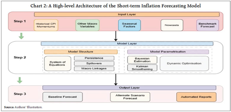

The benchmarks forecasts are atheoretical by design, making them an ideal reference point for nowcast to converge to. They reflect the information contained in historical patterns and derived out of model-imposed dynamics. This makes them particularly important within the broader forecasting framework – they act as the dynamic equilibrium/ benchmark.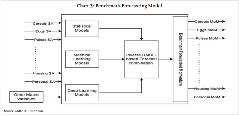

II.2. Model Layer (Short-term Forecasting Model): The Model Layer is the analytical engine of our short-term forecasting framework. It is a semi-structural model incorporating persistence, spillovers, and macro-linkages. It transforms the inputs into forecasts through Bayesian posterior updation, Kalman filtering and dynamic optimisation. This layer is bifurcated into two subsystems: Model Structure, and Model Parametrisation and Estimation. Model structure in sub-section (a) describes the equations in STFM, which are characterised by persistence, macro-linkages and interlinkages among the various CPI sub-groups/ components. Model Parametrisation and Estimation in sub-section (b) describes the parameter estimation process.

a) Model Structure: Inflation dynamics is modelled with a set of transition equations specified for each of the 33 CPI sub-groups/components, allowing each category to respond to its own persistence, spillovers from other components (say passthrough effects from fuel prices and cost-push pressures), macro-linkages (say exchange rate passthrough to inflation and demand sensitivity) and idiosyncratic shocks. For each sub-group, inflation is governed by a system of identities and behavioural equations, such as identities linking the seasonally adjusted momentum and seasonal factors; closing identities for seasonal factors and benchmark forecasts; and dynamic behavioural equations capturing the evolution of seasonally adjusted momentums. The behavioural equations are specified as a function of lagged inflations (capturing intrinsic persistence), exogenous macro drivers (e.g., output gap, cost-push pressures and exchange rate movements), spillover effects from other sub-groups/components, benchmark forecasts, and stochastic shocks. The set of equations are as below:

For all elements in

Var = {‘Cereals & products’, ‘Pulses & products’, ‘Milk & products’, ‘Eggs’, ‘Meat & Fish’, ‘Vegetables’, ‘Fruits’, ‘Spices’, ‘Oil & Fats’, ‘Sugar & confectionary’, ‘Non-Alcoholic Beverages’, ‘Prepared meals’, ‘Electricity’, ‘LPG’, ‘Kerosene-PDS’, ‘Kerosene-Other’, ‘Diesel’, ‘Other fuel’, ‘Coke’, ‘Firewood & chips’, ‘Coal’, ‘Charcoal’, ‘Dung cake’, ‘Housing’, ‘Pan, Tobacco & Intoxicants’, ‘Clothing’, ‘Footwear’, ‘Household’, ‘Health’, ‘Transport & communication’, ‘Recreation & amusement’, ‘Education’, ‘Personal care & effects’}

^DLVar{i} is the m-o-m per cent change in the i^th variable in Var.

^DLVar{i}_SA is the seasonally adjusted m-o-m per cent change in the i^th variable in Var.

^DLVar{i}_SF is the seasonal factors of the m-o-m per cent change in the i^th variable in Var.

^DLVar{i}_BM is the benchmark forecasts of the seasonally adjusted m-o-m per cent change in the i^th variable in Var.

OG and Ex are output gap and exchange rate, respectively.

Equation (1) represents the identity linking seasonally adjusted and unadjusted series. Equations (2) and (3) are used for closing the model structure. The benchmark forecasts (^DLVar{i}_BM) and seasonal factors (^DLVar{i}_SF) in the entire forecast horizon are provided as exogenous inputs. Equation (4) represents the behavioural equation encompassing persistence, spillovers, and macro impacts, which allows the convergence from nowcasts (initial condition) to the benchmark forecasts. The dimension of the short-term forecasting model is presented in Table 1.

b) Model Parametrisation and Estimation: The model parameters are estimated using Bayesian techniques. The unobserved variables are filtered out using Multivariate Kalman Filter. Using the estimated posterior parameters and initial conditions, as provided by nowcasts, the h-period ahead forecasts are then generated using dynamic optimisation.

The Bayesian estimation is carried out using the Metropolis-Hastings⁶-Markov Chain Monte Carlo⁷ (MH-MCMC) method. For each parameter in the model, a prior distribution is specified as lognormal distribution centred around a prior mode, which are identified using single equation econometric methods. The MH algorithm iteratively draws from the proposed distribution and accepts or rejects samples based on the posterior likelihood, eventually converging to the target posterior modes as defined by Bayes’ rule. The estimation is governed by a set of convergence criteria, including tolerances on function values, subject to constraints and bounded by a maximum number of iterations. Once the posterior sampling is completed, the posterior modes are computed from the MCMC draws and stored for subsequent use in filtering and forecast generation. An adaptive random-walk Metropolis (ARWM) posterior simulator⁸ is used to draw samples from the prior distribution and uses estimated posterior modes to generates a large chain of iterations (here 5,00,000) to reach stationary posterior distributions. These distributions are used to generate 95 per cent credible intervals (CI)⁹. Further, the unobserved variables are filtered out using multivariate Kalman smoothing procedure¹⁰. Then, through a dynamic optimisation process¹¹, the estimated system guides nowcasts towards the benchmark forecasts, which provide the point forecasts for each of the components and groups. Further, density forecasts for each of the variables are generated using multivariate and time-simultaneous prediction bands¹². Here, the forecast mean square error matrices are used to generate the forecast error standard deviations (SD), which in turn is applied on the point forecasts to obtain the density forecasts, assuming a normal distribution¹³.

II.3. Output Layer: The Output Layer forms the final stage of the forecasting system, transforming the forecasted momentum (expressed in m-o-m per cent change) paths of each of the 33 CPI sub-groups/ components—generated in the Model Layer—into forecasts of indices, year-on-year (y-o-y) inflations and contributions.

The momentum forecasts are applied to the one-period prior observed/estimated indices to recursively construct the forecasted indices for each component/ sub-group. These are then aggregated into broader categories¹⁴,—’Food & Beverages’, ‘Fuel & Light’, and ‘Core’ (Ex-Food & Fuel)—using CPI weights. ‘Fuel & Light’ sub-group, provides an additional challenge due to the aggregation biases¹⁵. Hence, for ‘Fuel & Light, an additional refinement is introduced. The weighted statistical moments (variance, skewness, and kurtosis) of the constituent fuel items are used as predictors for estimating the aggregation biases. From the forecasted indices, the y-o-y inflation and m-o-m rates for each sub-groups/components and at aggregated (groups and headline) levels are then calculated.

A toolbox has been developed in Matlab^®, using the IRIS¹⁶ and MikTex^©17 to support the model estimation, forecasting and output generation – including forecast tables and charts – compiled into a publication-ready report.

III. Results

The estimated parameters and 95 per cent CI are provided in Table 2.

The impact of some key macro variables on headline y-o-y inflation can be derived from this framework (Chart 4). This includes both direct and indirect effects.

Ten per cent depreciation in exchange rate leads to around 80 basis points (bps) increase in inflation over a period of 12 months (Chart 4.a). If demand conditions increase by 1 per centage point (ppt), headline inflation increases by close to 20 bps over a period of one year (Chart 4.b). The ten per cent increase in diesel (pump) prices, will lead to an increase in the headline inflation by around 90 bps over a 12-month horizon (Chart 4.c).

Using one of the components as an example, Chart 5 illustrates the convergence of nowcast at period (t+0) to the benchmark forecast at horizon (t+11), generated from the short-term forecasting framework. This chart indicates that the nowcast (red triangle marker, Chart 5) of this component estimated from the high-frequency data is largely different from that emerged out of the benchmark forecast at (t+0) (dotted black line, Chart 5). Using nowcast as the initial condition, the short-term forecasting model allow nowcast to converge to the benchmark forecast (red dotted line, Chart 6). Here, it could be interpreted that in case of this sub-component, the difference in the near-term is largely transitory. However, the persistence, spillovers, and macro-linkages has slowed down the convergence of momentum forecast to benchmark forecast, even after 12-months, thus, leaving some lasting impact.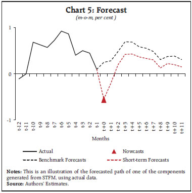

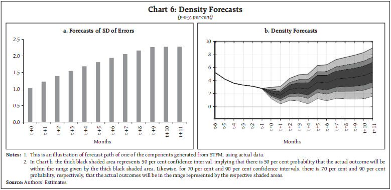The SDs of the forecast errors for each sub-group/ component that are also generated from this framework, are then used for creating the density forecasts. An illustrative example of a group in CPI basket is demonstrated in Chart 6. Chart 6.a provides the uncertainty around the point forecasts through horizons, which are measured using SDs. Estimated SDs are then used to generate the density forecast (Chart 6.b).

Finally, the evaluation of the short-term forecasting model is carried out by generating pseudo-out of sample root mean square errors (RMSE) (Chart 7).

Pseudo-out of sample RMSE for y-o-y headline inflation is markedly lower in the near-term compared to benchmark forecasts indicating the advantage of full information based nowcasts in the near-term. As the horizon extends the accuracy of the short-term forecasts converges to that of the benchmark forecasts. The advantage of the benchmark model (based on inflation combination approach of a large suite of models) in terms of accuracy for generating forecasts in short-term horizon, relative to other models is already established in the Indian context (Mohan et al., 2025). Thus, the proposed framework leverages the advantage of nowcasts in the near-term, while ensuring enhanced forecast accuracy in the short-term. However, the overall accuracy of this framework depends on the accuracy of the nowcasts. This underscores the need for a consistent and accurate framework for generating nowcasts, rather than the full information matrix–based system presented in this article. Ideally, such a framework should integrate high-frequency, spatial, and multi-source data sets–an area identified for future research.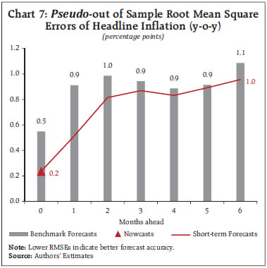

IV. Conclusion

This paper presents a framework for short-term inflation forecasting that bridges data-driven modelling, machine learning techniques, structural hysteresis, macro-linkages, and inter-sectoral spillovers. By integrating nowcasts, benchmark forecasts, seasonal factors, and judgmental adjustments into a dynamic system of disaggregated component/sub-group level equations, this framework offers a forward-looking and granular view of inflation dynamics. The design’s flexibility also enables scenario analysis. Importantly, the disaggregated architecture allows for clear attribution to inflation formation. In this framework, the enhanced forecast performance in the near-horizon stemming from nowcasts is accounted for, still preserving the advantage of statistical and machine learning models in short-horizon. It is also equipped with generating density forecasts. As such, this forecasting framework provides a powerful, yet pragmatic solution for generating short-term inflation forecasts, in an increasingly complex and uncertain environment, which are peculiar characteristics of an emerging market economy.

References:

Barratt, S. T., & Boyd, S. P. (2020, July). Fitting a Kalman smoother to data. In 2020 American Control Conference (ACC), 1526-1531. IEEE.

Brooks, S. (1998). Markov chain Monte Carlo method and its application. Journal of the royal statistical society: series D (the Statistician), 47(1), 69-100.

Das, P. & George, A. (2023). Consumer Price Index: The Aggregation Method Matters. RBI Bulletin, March.

Del Negro, M., & Schorfheide, F. (2013). DSGE model-based forecasting. In Handbook of economic forecasting (Vol. 2), 57-140. Elsevier.

Eberhart, R., & Kennedy, J. (1995, October). A new optimizer using particle swarm theory. In MHS’95. Proceedings of the sixth international symposium on micro machine and human science, 39-43. IEEE.

Haario, H., Saksman, E., & Tamminen, J. (2001). An Adaptive Metropolis Algorithm. Bernoulli, 223-242.

Hastings, W. (1970). Monte Carlo sampling methods using Markov chains and their applications. Biometrika, 57(1), 97-109.

John, J., Singh, S., & Kapur, M. (2020). Inflation Forecast Combinations: The Indian Experience. Reserve Bank of India Working Paper Series No. 11.

Kolsrud, D. (2007). Time-simultaneous prediction band for a time series. Journal of Forecasting, 26(3), 171-188.

Lucas Jr, R. E. (1976, January). Econometric policy evaluation: A critique. In Carnegie-Rochester conference series on public policy (Vol. 1), 19-46. North-Holland.

Metropolis, N., Rosenbluth, A. W., Rosenbluth, M. N., Teller, A. H., & Teller, E. (1953). Equation of state calculations by fast computing machines. The journal of chemical physics, 21(6), 1087-1092.

Mohan, R., Hasan, S., Roy, S., Sarkar, S., and John, J. (2025) Predicting CPI inflation in India: Combining Forecasts from a ‘Suite’ of Statistical and Machine Learning Models, RBI Bulletin, June.

Monsell, B. C., Lytras, D., & Findley, D. F. (2016). Getting Started with X-13 ARIMA-SEATS Input Files. US Census Bureau. Center for Statistical Research and Methodology, ML.

^{^} The authors are from the Department of Statistics and Information Management, Reserve Bank of India. The views expressed in this article are those of the authors and do not represent the views of the Reserve Bank of India.

¹ In recent times, high frequency models of macro-linkages are gaining prominence e.g., Bayesian Machine Learning models and Gaussian Process and Bayesian Additive Regression Tree (BART). However, these models also, are dependent on data.

² Dynamic equilibrium is a state where a system is balanced, the macroscopic properties remain stable, even though changes are occurring at microscopic level.

³ Along with the officially classified 22 CPI sub-groups, 11 ‘fuel’ items are also considered in the model framework separately. Thus, the 33 sub-groups/ components are ‘Cereals & products’, ‘Pulses & products’, ‘Milk & products’, ‘Eggs’, ‘Meat & Fish’, ‘Vegetables’, ‘Fruits’, ‘Spices’, ‘Oil & Fats’, ‘Sugar & confectionary’, ‘Non-Alcoholic Beverages’, ‘Prepared meals’, ‘Electricity’, ‘LPG’, ‘Kerosene-PDS’, ‘Kerosene-Other’, ‘Diesel’, ‘Other fuel’, ‘Coke’, ‘Firewood & chips’, ‘Coal’, ‘Charcoal’, ‘Dung cake’, ‘Housing’, ‘Pan, Tobacco & Intoxicants’, ‘Clothing’, ‘Footwear’, ‘Household’, ‘Health’, ‘Transport & communication’, ‘Recreation & amusement’, ‘Education’, and ‘Personal care & effects’.

⁴ X-13ARIMA-SEATS is seasonal adjustment software produced, distributed, and maintained by the US Census Bureau (For reference material see Monsell, Lytras and Findley, 2016).

⁵ In a pseudo out-of-sample forecasting exercise, the forecasts are generated at time t-h (for h = 1 to m) in the past, using only the data available till that time (t-h) for parametrisation of the model as well as for generating the forecast of the exogenous and endogenous variables.

⁶ MH algorithm (Metropolis et al., 1953; Hastings, 1970) is the most popular technique to build Markov chains (series of dependent samples) with a given invariant distribution. While Metropolis et al. (1953) requires that the proposed distribution be symmetric, Hastings (1970) generalises it to allow asymmetric distributions.

⁷ MCMC methods generate Markov chains, which over time converges to a desired stationary distribution. This method is used for approximating complex distributions and estimating its parameters, even when theoretical closed-form solutions are unavailable. For details, refer to Brooks (1998).

⁸ In ARWM, a proposed distribution (here Normal) is updated adaptively using the full information accumulated so far. Due to its adaptive nature the ARWM algorithm is non-Markovian, however it has the right ergodic properties. ARWM, thus overcomes the issue of the choice of a proper distribution, which is vital for the convergence in the traditional MCMC algorithms (Haario et al., 2001).

⁹ Credible intervals are intervals generated from the posterior probability density function. It can be interpreted similar to the confidence interval in the frequentist approach. For e.g., a 95% credible interval is having 95 per cent probability that the true value of the estimate would lie within that interval.

¹⁰ Multivariate Kalman filter uses observed variables and stochastics noises over time to filter out unknown variables, using a multivariate state-space model, which applies the joint probability distributions in each time-step. This system level approach tends to be more accurate than those based on a single measurement variable and a single equation. A Kalman smoothing process uses both past and future values and tend to be even more accurate. For details, refer to Barratt and Boyd (2020).

¹¹ Dynamic optimisation involves the following steps: 1) steady state solutions are obtained using Newton-type algorithm, 2) dynamic solutions, which guides the disequilibria at any time to the steady state, are obtained using particle swarm optimizer (Eberhart and Kennedy, 1995). 3) The point forecasts are then generated using equation-selective simulator with Shanks acceleration (a non-linear algorithm which improves the rate of convergence).

¹² Multivariate and time-simultaneous prediction bands aim to capture possible outcomes for all variables at all horizons within any specified confidence level. This is used to forecasts confidence bands of different related time series by simultaneously considering the temporal uncertainty as well as their interlinkages across different variables. These are generated by estimating forecast mean square error matrices (Kolsrud, 2007).

¹³ The framework can also be used to generate asymmetric confidence interval forecasts using a split-normal distribution.

¹⁴ The 33 component/sub-group level indices are aggregated into three respective groups (Food, Fuel and Core) using the CPI-C weights. Subsequently, headline index is calculated using the group-wise CPI-C weights.

¹⁵ The weighted vertical aggregation of the item-level indices does not match with the published ‘Fuel & Light’ index (Das and George, 2023).

¹⁶ IRIS is an open-source toolbox for macroeconomic modelling and forecasting in Matlab^®, originally developed by the ‘IRIS Solutions Team’ and currently maintained and supported by the ‘Global Projection Model Network’. https://iris.igpmn.org/

¹⁷ MikTex^© is an open-source TeX /LaTeX editor for creating, typesetting, and previewing documents.