by Renjith Mohan, Saquib Hasan, Suvendu Sarkar and Joice John^ This article examines the drivers of headline inflation1 volatility in India. The main source of this volatility is emanating from vegetable prices–especially that of tomato, onion, and potato (TOP)–along with spillovers from non-TOP vegetable prices. Volatility has eased under the flexible inflation targeting (FIT) framework relative to the pre-FIT period, even amid repeated supply shocks. Since 2021, a major contributor to this moderation has been the government’s timely, targeted supply-side interventions, which helped dampen commodity-specific price spikes. Overall, India’s inflation management reflects a coordinated strategy where fiscal actions curb extreme price movements, while monetary policy anchors expectations and limits the broader transmission of relative price shocks. Introduction Inflation volatility poses significant challenges for macroeconomic stability, particularly in emerging economies like India, where price fluctuations are driven by a complex interplay of supply shocks, policy changes, and structural rigidities. While inflation targeting framework anchor inflation expectations, managing short-term volatility continues to remain a formidable challenge. Consumer Price Index (CPI) (2012=100) basket in India is structurally predisposed for heightened inflation volatility due to the significant weight assigned to food, which is highly sensitive to supply-side shocks. This composition of high weightage for food (45.9 per cent of the overall CPI basket (2012=100)), exposes headline inflation to heightened volatility. Food prices exhibit substantial volatility mostly driven by weather fluctuations, disruptions in supply chains, and policy interventions such as export/import restrictions, changes in duties and minimum support prices. Fiscal interventions– including buffer stock releases, tax adjustments, and export restrictions– play an important role in stabilising prices. Further, monetary policy actions also have a role in containing inflation volatility. Price volatility in certain commodities may transmit to other items. A prudent monetary policy can contain this volatility spillover. Against this backdrop, the present study aims to identify and categorise the drivers of CPI headline inflation volatility in India during the FIT period (2016–2025), with particular emphasis on the role of food prices and the dynamics of volatility transmission. By combining cross-sectional distributional measures of inflation with spillover analysis and incorporating government interventions into an analytical framework, this paper seeks to provide a comprehensive assessment of the mechanisms that shaped the retail inflation volatility in India. Section II reviews the existing literature on inflation volatility and food price dynamics; Section III presents some stylised facts on temporal and cross-sectional distribution of headline inflation volatility; Section IV outlines the methodological framework and empirical findings; and Section V concludes with policy implications. II. Literature Review The relationship between relative price movements and aggregate inflation has long been central to macroeconomic analysis. Ball and Mankiw (1995) argued that inflation cannot be understood simply as the average of relative price changes but is influenced by the distribution and variability of those changes. Large shocks in key sectors such as food and energy can transmit beyond their immediate impact, creating aggregate inflationary pressures. They further emphasised on how the distributional characteristics of shocks also play an important role in price variability mapped through the asymmetry in price changes quantified by skewness. This framework provides a theoretical foundation for linking relative price volatility to headline inflation, particularly in economies where food carries substantial weight in the consumption basket and exhibits distinctive price behaviour compared to non-food items. In this context, Walsh (2011) explored the characteristics of food and non-food inflation across countries and highlights that food inflation in many low- and middle-income economies tends to exhibit greater persistence and volatility and detailed the importance of recognising multiple transmission channels through which food prices could influence non-food inflation. Cecchetti and Moessner (2008) also examined the implications of rising global commodity prices and found how food prices are aiding in shaping headline inflation patterns, suggesting the need for a broader inclusive approach to inflation monitoring. In the Indian context, several studies have documented the multi-factorial nature of food inflation. Gulati and Saini (2013) identified various macroeconomic and structural drivers such as fiscal imbalances, rising input costs, and shifts in consumption patterns. Dua and Goel (2021) emphasised the role of demand-side and supply-side interactions–including inflation expectations, minimum support prices, and rainfall conditions. Sasmal (2015) presented a general equilibrium approach to highlight the sectoral asymmetries contributing to food price pressures. Further, Gulati and Wardhan (2019) pointed to the influence of supply chain frictions and post-harvest losses in intensifying price volatility in perishable items like vegetables. Bhattacharya and Gupta (2015) had found that both supply and demand factors drive food inflation in India with wages, input costs and support prices playing key roles. A focused strand of literature has examined the dynamics of price movements in key vegetables– specifically Tomato, Onion, and Potato (TOP)–which are known to exhibit sizable short-term volatility. Roy et al. (2024), provided a detailed empirical analysis of the supply-demand and price behaviour of TOP items, using a balance-sheet framework and time-series modelling. Their findings highlighted the influence of market arrivals, climatic factors, and infrastructural limitations on price formation. Kishore and Shekhar (2022) assessed the role of extreme weather events and showed that unseasonal rains and cyclones in major producing states had been associated with sharp price movements in TOP vegetables, with implications for inflation forecasting accuracy. The impact of climatic variability on vegetable prices is further elaborated by Singh and Shandilya (2025), who analysed how anomalies in rainfall and temperature patterns influence vegetable inflation in general. Their results underscored the rising significance of temperature shocks and the need for incorporating weather indicators into food price monitoring frameworks, especially under a flexible inflation targeting (FIT) regime. Patra et al. (2024a, 2024b) offered a careful examination of the changing role of food inflation in India’s overall inflation dynamics and suggested that food prices, traditionally viewed as volatile but transitory, are increasingly displaying persistence. This persistence, they argued, reflects the cumulative impact of repeated supply-side shocks, many of which are climate related. Episodes of unseasonal rainfall, heatwaves, and other weather anomalies have disrupted production cycles and supply chains, thereby introducing more systematic, rather than purely episodic, price pressures. In addition to documenting this food inflation behaviour, Patra et al. (2024b) explored its transmission to broader macroeconomic variables. They found that persistent food price shocks also influenced household inflation expectations, raising the risk of second-round effects through wage demands and price-setting behaviour in the non-food sector. Patra et al. (2024c) extended this discussion by analysing how fiscal interventions interacted with cross-sectional distributional features of inflation, namely volatility and skewness. Their findings highlight that repeated supply-side shocks in food and fuel amplified inflation variability, and that government measures–such as buffer stock management and import/export policies–helped to mitigate these effects. While their analysis incorporated both volatility and skewness, the volatility dimension is particularly relevant here, as it illustrates how supply-side interventions can complement the role of monetary policy in stabilising inflation outcomes during periods of heightened uncertainty. All these reflect a growing recognition of the importance of food price dynamics, their broader implications for inflation volatility and monetary policy formulation in India. The present study builds upon these insights by examining the intra-group volatility patterns within food inflation, focusing on the role of certain items/sub-groups. This study aims to contribute to the existing literature with a specific focus on the role of key sources and determinants of inflation volatility, a topic that was touched upon in previous articles but warrants a deeper investigation. We further examine how the spillover effects shaped the headline inflation variability in India and was affected by the supply-side interventions by the Government of India (GoI). III. Stylised Facts The temporal distribution of the headline inflation (year-on-year) during 2016-20252 reveals that the distribution remained broadly symmetrical with mean at 4.9 per cent and standard deviation at 1.5 per cent (Chart 1). Headline inflation volatility, as measured by the standard deviation in 12-month rolling window, exhibited a significant reduction from 2.4 per cent in the pre-FIT period (2012–2016) to 1.5 per cent during (2016–2025). Notably, during this period, inflation exceeded the upper tolerance threshold of 6.0 per cent in 26 per cent of the months, while it fell below the 2.0 per cent lower bound only three times. Inflation volatility at the sub-group level (characterising the cross-sectional variation and measured by sub-group level standard deviations) reveals a marked divergence between food and non-food components, with food inflation exhibiting higher volatility compared to its non-food counterparts (Chart 2). However, this pattern was not uniform across all food sub-groups. Specifically, items such as ‘vegetables,’ ‘pulses,’ ‘spices,’ and ‘oils and fats’ displayed higher volatility, whereas ‘milk,’ ‘prepared meals,’ and ‘beverages’ showed relatively lower volatility on an average. This suggests that the observed volatility in food inflation was not a generalised phenomenon rather driven by specific sub-groups within the food category.
Taken together, these distributional patterns suggest that headline inflation volatility is driven by a small subset of components within food, warranting a systematic decomposition of variance and assessment of volatility spillovers. IV. Empirical Results In this section, we present the sources, determinants, and effects of inflation volatility. The approach encapsulates the following analysis: i) the decomposition of temporal headline inflation volatility to group/subgroup-level volatility and covariance among them (Borio, et al., 2023) revealing the key determinants of headline inflation volatility; ii) using generalised forecast error variance decomposition the channels of volatility spillovers (Borio et al., 2023) are identified iii) relationship of the higher order moments of inflation with headline inflation (Ball and Mankiw, 1995) are estimated ; and iv) the role of supply-side interventions by GoI on headline inflation and its volatility are examined. IV.i. Sources of Inflation Volatility: Decomposition of Variance in Headline Inflation In this section we decompose the temporal volatility in headline inflation to its components emanating from sub-group level volatilities and the covariance among them. Variance of headline inflation3 can be decomposed into those from individual sub-groups and covariances among them (Borio et al. 2023). The results indicate that the variance of headline inflation remained relatively stable over time, except during 2019–2020 (Chart 3). The reduction in inflation volatility observed from 2019–2023 can be primarily attributed to a decrease in the covariance among the sub-groups. Since 2022-23, the contribution by the covariance among the sub-groups turned negative. This period coincided with the tightening of monetary policy. The behaviour of inflation volatility during this period reflects the decoupling of price movements across sub-groups, rather than broad-based shifts in overall price levels. However, inflation volatility increased during 2023-2025 primarily due to the increase in volatility in vegetable prices. In 2025-26 (till Aug-25), more than 80 per cent of variation in headline inflation is attributed to vegetable prices. However, these heightened volatilities in sectoral inflations had not translated to higher covariances and further amplification of headline inflation volatility. This suggest that while price changes at the sub-group level exhibited variability, these fluctuations were largely idiosyncratic and not correlated indicating restricted volatility spillovers. 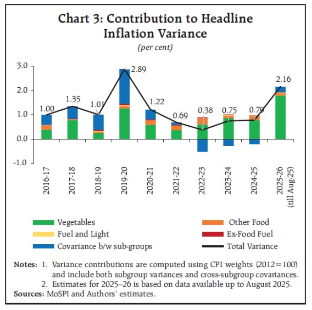 Now we turn on to analyse the volatility of inflation in vegetables to identify its determinants (Chart 4). The findings underscore the role of sporadic and episodic price shocks, particularly in the ‘Tomato- Onion-Potato’ (TOP) category, which had been a major contributor to the volatility in ‘vegetables’ inflation. Notable instances of such shocks inducing volatility include onion prices during 2019-20, potato prices in 2020-21, and tomato prices in 2022-23, 2023-24, and 2024-25. However, it is observed that the covariances among the items within the ‘vegetables’ sub-group accounted for more than 50 per cent of the total volatility in ‘vegetables’ inflation across the examined period, even higher than 65 per cent in 2025-26. This suggests the presence of significant volatility spillovers among these items. The price fluctuations in one vegetable item may transmit to other items in the sub-group, thereby, amplifying the volatility in overall vegetable inflation. This inter-dependence among vegetable price volatility further complicates efforts to isolate the sources and underscores the importance of volatility spillovers while analysing inflation volatility at sub-group level. 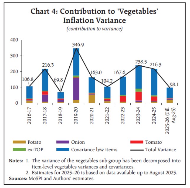 Reading all together, we can conclude that the sporadic and episodical shocks in TOP prices and the covariance among the vegetable prices are responsible for the overall headline volatility. For isolating the specific shocks in vegetable prices that bring in this heightened volatility, we need to identify the determinants of volatility in vegetable price inflation. IV.ii. Determinants of Volatility in Vegetable Prices To capture intra-group determinants of vegetable inflation volatility, a Vector Autoregression (VAR) framework was employed (Borio et al., 2023) on the monthly percentage changes of six components of CPI vegetable sub-group (Tomato, Onion, Potato, Garlic, Ginger and ‘Other Vegetables’) using the data from April 2015 onwards (till August 2025). Tomato- Onion-Potato (TOP) are known for sporadic price changes; Garlic and Ginger, exhibit distinct seasonal behaviour and are storable, while ‘Other Vegetables’ comprise the remaining items in the sub-group. This classification facilitates measurable identification of origins and directions of volatility spillovers within the vegetable basket. To quantify these spillovers, we employ the Generalized Forecast Error Variance Decomposition (GFEVD)4 at horizon H, following the methodology proposed by Diebold and Yilmaz (2012). The GFEVD decomposes the forecast error variance of each variable into components attributable to its own shocks and to those emanating from other components. 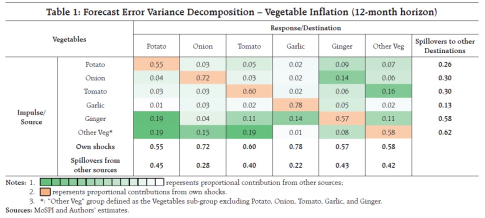 The results from the GFEVD analysis, conducted over a 12-month horizon, indicate a distinct asymmetry in the transmission of shocks within the ‘vegetables’ sub-group (Table 1). Shocks to the prices of ‘Tomato-Onion-Potato’ exhibit a lower propensity to generalize compared to shocks originating from ‘other vegetables.’ In contrast, volatility in the prices of ‘other vegetables’ tends to transmit to the prices of TOP items, thereby inducing volatility in the latter. Further, shocks in TOP prices are not found to be mutually spilling among themselves. These results indicate that even though the contribution of item-specific shocks of ‘ex-TOP vegetable’ prices to overall ‘vegetable’ inflation volatility is relatively small, they have the potential to generalise and amplify the volatility to ‘vegetables’ sub-group as a whole, through spillovers. As volatility in headline inflation is largely driven by volatility in ‘vegetables’ inflation, we can now conclude that the volatility in headline inflation is mainly determined due to the sporadic and episodical shocks in prices of ‘Tomato-Onion-Potato’ (TOP) and spillovers emanating from the volatility in prices of ‘ex-TOP’ vegetables. Now we turn on to the implications of volatility for inflation management. IV.iii. Impact of Volatility and Asymmetry on Inflation In this section we assess whether the distributional moments – standard deviation (σt) and skewness (γt) affects changes in headline inflation (Ball and Mankiw, 1995). The regression specification is as follows: Δπt = α + β1Δπt–1 + β2 Δσt + β2 Δγt + εt (1) where, Δπt is the change in seasonally adjusted annualised headline inflation. As vegetables are the main contributor of headline inflation volatility, alternatively we use the volatility (σvt) and skewness (γvt) for vegetables in the regression equation (1). The regression estimates provided in Table 2 (model 2 and 3) clearly indicates that cross-sectional volatility and skewness play a significant role in driving the headline inflation dynamics in India. For the headline CPI, the coefficient on inflation volatility and skewness is positive and statistically significant. This aligns with the theoretical framework of Ball and Mankiw (1995), who emphasised that inflation reflects not only average relative price changes but also their variability. This is also in line with the results of Patra et al. (2014) for India based on WPI. Put differently, when relative price shocks widen the distribution of sectoral inflation rates, they elevate headline inflation over and above the effect of average movements. The results suggest that India’s inflation trajectory has been particularly sensitive to the volatility dimension of relative prices, underscoring the persistent influence of food and other supply-driven shocks on aggregate inflation outcomes. | Table 2: Regression Results | | Sample Period: Apr-15 to Aug-25 | Dependent Variable: ∆πt | | (1) | (2) | (3) | (4) | (5) | | ∆πt–1 ∆σt ∆γt v Δσ t Δγ v t α | -0.22** | -0.25* | -0.26* | -0.27** | -0.22** | | (0.02) | (0.07) | (0.08) | (0.04) | (0.02) | | | 0.83** (0.03) | | | | | | | 1.30** (0.00) | | | | | | | 0.26** (0.00) | | | | | | | 0.29 | | | | | | (0.74) | | -0.18 | -0.38 | -0.31 | -0.35 | -0.19 | | (0.74) | (0.47) | (0.57) | (0.51) | (0.74) | | Diagnostics | | ARCH LM test p-value | 0.00 | 0.00 | 0.00 | 0.00 | 0.00 | | Breusch-Godfrey LM test p-value | 0.00 | 0.40 | 0.14 | 0.92 | 0.00 | Notes: 1. p-value are in brackets: * p<0.1, ** p<0.05
2. As the variables were found to be difference stationary, the estimation is carried out in the first difference.
3. p-values correspond to the robust standard errors in model 2, 3 and 4 and Newey-West errors in model 1 and 5.
4. As the null hypothesis of no ARCH effect is rejected in all models, this strengthens the case for GARCH model exploration.
Sources: MoSPI and Authors’ estimates. | Focusing specifically on the vegetables subgroup, the results reveal that volatility within this narrower basket also has a significant bearing on headline inflation (model 4 in Table 2). The positive and robust coefficient on vegetable volatility highlights that fluctuations in highly perishable and policy-sensitive items such as tomato, onion, and potato extend beyond their direct contribution to the overall index. By contrast, the skewness of vegetable inflation does not emerge as statistically significant, suggesting that it is the magnitude of dispersion, rather than asymmetry in the distribution of vegetable inflation that drives the transmission to aggregate inflation (model 5 in Table 2). Taken together, these findings reaffirm that headline inflation dynamics are shaped not only by average price changes but also by the cross-sectional volatility of its key components. Now, we turn on to the role of supply-side management in determining the inflation developments and volatility in India. IV.iv. Supply Side Measures by Government and Inflation Volatility Finally, we examine whether supply-side interventions conducted by GoI (a gist of some of the measures are provided in Annex Table I) had any impact on headline inflation and its variability. To quantify the fiscal supply-management actions, we construct an index of supply-side measures following Patra et al. (2024c). Specifically, we code a binary indicator (Git), that takes the value 1 when a supply-management intervention is undertaken for commodity i in month t, and 0 otherwise. The aggregate index is then computed as a CPI-weighted (2012=100) sum across commodities, i.e. Gt = Σiwi Git, where wi denotes the CPI basket weight of select item i5 (Chart 5). This procedure yields a monthly measure of the extent of targeted supply-side actions–such as import facilitation, export restrictions, stock limits, and buffer stock releases–allowing us to estimate how such interventions interact with inflation dynamics and volatility. We estimate GARCH (1,1) where distributional moments and their interaction with interventions affect both the level and conditional volatility of headline inflation. Mean equation: Δπt = α + β1 Δπt–1 + β2 ΔMt + β3 (ΔMt × ΔGt) + εt (2) Volatility equation: ht = ρ + ρ1 ΔMt + ρ2 (ΔMt × ΔGt) + ρ3 ε2t –1 + ρ4 ht–1 (3) where, ht is the conditional variance of inflation at time t, ε2t –1 provides the ARCH term and ht–1 is the GARCH term. Substituting Mt = σ t yields the cross-sectional volatility-based equation, while Mt = γ t yields the cross-sectional skewness-based equation. This formulation aids in measuring how supply side measures interact with distributional features of headline inflation and its effects on inflation volatility. Results in Table 3 show that even though the cross-sectional volatility is not statistically significant in the mean equation (after the inclusion of ARCH/ GARCH terms), its interaction with the index of supply-side measures is statistically significant and negative. This suggests that supply side measured effectively dampened the ill effects of heightened volatility on headline inflation. In the variance equation, as expected, cross-sectional volatility is positive and statistically significant, confirming that relative price dispersion magnifies the temporal inflation variability. Here again, the interaction with supply-side measures is negative and significant, implying that interventions were successful in containing the inflation volatility. Taken together, these findings reflect the food supply management measures by GoI not only successfully muted the inflationary effects of adverse supply-side shocks but also prevented the volatility spillovers. 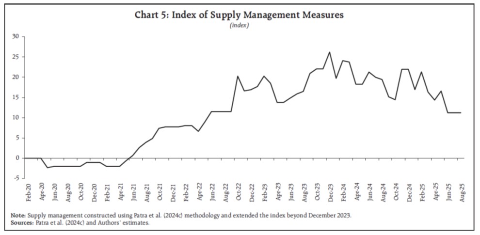
| Table 3: Regression Results: GARCH Model | | Sample Period: Feb-20 to Jul-25 | (1) | (2) | | Mean Equation Dependent Variable: ∆πt | | ∆πt–1 | -0.19* | -0.24** | | | (0.07) | (0.04) | | ∆σt | 0.578 | | | | (0.13) | | | ∆γt | | 0.97** | | | | (0.04) | | ∆σt × ΔGt | -0.21** | | | | (0.01) | | | ∆γt × ΔGt | | -0.13 | | | | (0.43) | | α | 0.51 | 0.18 | | | (0.43) | (0.79) | | Variance Equation Dependent Variable: ht | | | ∆σt | 0.22** | | | | (0.03) | | | ∆γt | | 0.54** | | | | (0.00) | | ∆σt × ΔGt | -0.10* | | | | (0.08) | | | ∆γt × ΔGt | | -0.04 | | | | (0.60) | | ρ | 2.29** | 2.65** | | | (0.00) | (0.00) | | ARCH/GARCH | | ARCH (1) | 0.12 | 0.20* | | | (0.23) | (0.08) | | GARCH (1) | 0.35 | 0.28 | | | (0.14) | (0.11) | p-values are in brackets and are robust (Huber–White type); * p<0.1, ** p<0.05
Sources: MoSPI and Authors’ estimates. | Limitations and Scope for future Work: This article examines a more aggregated picture of temporal and broader sub-groupwise sources of headline inflation volatility. However, inflation volatility can emanate from dis-aggregate sources often rooted in product-specific (based on perishability), spatial (production versus consumption centres and supply chains), and temporal (weather related anomalies) characteristics. Future work could incorporate a more disaggregated approach focusing on these key drivers of volatility. IV. Conclusion The analysis reveals that much of the volatility in headline inflation emanates from the vegetables, driven by sharp and sporadic shocks to 'Tomato– Onion–Potato' (TOP) prices and amplified by spillovers from ‘ex-TOP’ vegetables. Further, the headline inflation volatility moderated during the period from 2016–2025, even in the face of substantial supply-side shocks. The decline in volatility since 2021–2022 is closely associated with a reduction in sectoral covariance and sectoral price shocks no longer broadly propagate across the inflation basket. This indicates that under the FIT regime, inflation expectations remain anchored. The regression analyses suggest that while cross-sectional volatility is the key driver of temporal inflation variability, its adverse effects are significantly mitigated by supply-side interventions by the government (such as buffer stock releases, trade adjustments, and import facilitation). In particular, these interventions have been effective not only in dampening immediate inflationary pressures but also in curbing the volatility in inflation. For an emerging economy like India, where food accounts for a large share in CPI basket and food prices are highly vulnerable to weather shocks and supply disruptions, these findings carry important policy implications – price stability can be achieved efficiently by effective monetary and fiscal coordination. References Ball, L. and N G Mankiw (1995). Relative-price Changes as Aggregate Supply Shocks, Quarterly Journal of Economics, Vol 110, No 1, pp 161–93. Bhattacharya, R., and Gupta, A. S. (2015). Food Inflation in India: Causes and Consequences. National Institute of Public Finance and Policy. Working Paper, 151. Borio, C., Lombardi, M., Yetman, J., and Zakrajšek, E. (2023). The two-regime View of Inflation. BIS Papers. Cecchetti, S., and Moessner, R. (2008). Commodity Prices and Inflation Dynamics. BIS Quarterly Review. Diebold, F. X., and Yilmaz, K. (2012). Better to Give than to Receive: Predictive Directional Measurement of Volatility Spillovers. International Journal of Forecasting, 28(1), 57–66. Dua, P., and Goel, N. (2021). Determinants of Inflation in India: A Structuralist Approach. Delhi School of Economics Working Paper. Gulati, A., and Saini, S. (2013). Taming Food Inflation in India. ICRIER Working Paper No. 279. Gulati, A., and Wardhan, H. (2019). Post-Harvest Losses and Value Chain Inefficiencies in India. ICRIER. Kishore, V., and Shekhar, H. (2022). Extreme Weather Events and Vegetable Inflation in India. Economic and Political Weekly, Vol LVII Nos 44 and 45. Patra, M. D., J. K. Khundrakpam, and A. T. George, (2014), “Post-Global Crisis Inflation Dynamics in India: What has Changed?” in Shekhar Shah, Barry Bosworth and Arvind Panagariya eds. India Policy Forum 2013-14, Volume 10, Sage Publications, July. Patra, M. D., John, J., and George, A. T. (2024a). Are Food Prices the ‘True’ Core of India’s Inflation?. RBI Bulletin, January 2024. Patra, M. D., John, J., and George, A. T. (2024b). Are Food Prices Spilling Over?. RBI Bulletin, August 2024. Patra, M., Bhattacharyya, I., and John, J. (2024c). Pushing Back Post-pandemic Price Pressures: A Monetary-Fiscal Symphony. Economic and Political Weekly, 59. Roy, R., Gupta, S., Wardhan, H., Sarkar, S., et al. (2024). Vegetables Inflation in India: A Study of Tomato, Onion, and Potato (TOP). RBI Working Paper Series 08/2024. Sasmal, J. (2015). Uneven Growth and Food Price Inflation in India: A CGE Approach. Economic Modelling. Singh, N., and Shandilya, L. K. (2025). Impact of Weather Anomalies on Vegetable Prices in India. RBI Bulletin, May 2025. Walsh, J. P. (2011). Reconsidering the Role of Food Prices in Inflation. IMF Working Paper 11/71.
Annex Table 1: Some major supply-side measures by Government of India in
Food Commodities since 20236 | Time | Commodity | Action | Implementing Agencies | | 2023 (Ongoing) | Pulses | Tur and urad under ‘Free Import Category’; 0 per cent import duty on tur and urad | Department of Consumer Affairs (DoCA) | | 2023 | Pulses | Stock limits imposed on tur and urad under Essential Commodities Act | DoCA, State Governments | | 2023 | Chana | Chana buffer released as ‘Bharat Dal’; sold at Rs. 60/kg (1kg) and Rs. 55/kg (bulk). The prices were revised in late 2024. | NAFED, NCCF, Kendriya Bhandar, DoCA | | 2023 (Ongoing) | Multiple | Use of Price Stabilisation Fund (PSF) for buffer procurement and subsidised retail | DoCA, NAFED, NCCF | | July 2023 | Tomato | Procurement from AP, Karnataka, Maharashtra during supply disruption | NAFED, NCCF | | Aug 2023 | Tomato | Retail sale launched at Rs. 90/kg, later reduced to Rs. 40/kg via mobile vans | DoCA, NAFED, NCCF | | Aug 2023 | Onion | MEP of $800/ton imposed to curb exports | DGFT, Ministry of Commerce | | Sep 2023 | Onion | Onion buffer stock raised to 5 LMT; retail sales launched at Rs. 35/kg | DoCA, NAFED, NCCF | | Oct 2023 | Onion | Distribution via Railways, e-commerce, and mobile vans | DoCA, Indian Railways, NCCF, NAFED | | Oct 2023 | Rice | Export ban on non-basmati rice; MEP of $950/ton on basmati rice | DGFT, Ministry of Commerce | | Nov 2023 | Wheat | ‘Bharat Atta’ launched at Rs. 27.50/kg | DoCA, FCI, NAFED, NCCF, Kendriya Bhandar | | Nov 2023 - Mar 2024 | Wheat | Weekly e-auctions under OMSS(D); 101.5 LMT sale targeted | FCI, DoCA | | Sep 2024 | Onion | Onion buffer sales resumed; retail price capped at Rs. 35/kg | DoCA, NCCF, NAFED | | Sep–Oct 2024 | Onion | Extended distribution via Railways, e-commerce, cooperatives | DoCA, Railways, NCCF, NAFED, State Govts | | Dec 2024 and May 2025 | Wheat | Further revised down the stock limit on wheat. Stock limits extended till Mar-26 during May-25 | DoCA, FCI |
|