A moderate recovery characterised domestic macroeconomic conditions in 2015-16, set against a global economy struggling to gain traction. Notwithstanding anaemic external conditions combined with sudden swings in asset prices and capital flows on global cues, macroeconomic stability and external viability were sustained. Stimulating private investment and reinvigorating the banking sector while maintaining macroeconomic stability remain the key challenges in the year ahead. II.1 THE REAL ECONOMY II.1.1 Provisional estimates of the Central Statistics Office (CSO) indicate that a moderate recovery characterised macroeconomic conditions in 2015-16, with a slight pick-up in pace in the second half of the year despite the drag from slowing investment. Private final consumption remained the bedrock of domestic demand, expanding to contribute over half of the overall GDP growth. Ongoing fiscal consolidation restrained government consumption during 2015- 16. Net exports were muted by the still depressed global trading environment as in the preceding year; however, a turnaround in their contribution to the growth of aggregate demand occurred in the second half of the year. This was in part due to the pace of contraction of imports outpacing that of exports, and in part due to gains in net terms of trade. II.1.2 As regards aggregate supply, agricultural and allied activities were buffeted by headwinds from deficiencies in precipitation and coverage in both monsoon seasons during the year, as well as floods and cyclones in the southern region in Q3 and unseasonal rains and hail in the western region in Q4. That the sector managed to post positive growth in sharp contrast to a year ago – despite an absolute contraction in Q3 – attests to its growing resilience and weather-proofing, and the rising profile of horticulture and allied activities that are relatively less rain-dependent. Value added in industry gathered momentum, especially in the second half of 2015-16, with the large boost provided by the decline in input costs offsetting the stalling evolution of industrial output and more recently, on sales growth. Activity in the services sector maintained a stable pace of expansion across constituents, although financial services, real estate and professional services experienced some slackening of pace in the second half. Overall, domestic economic activity was shored up by macroeconomic stability as reflected in falling inflation and narrowing current account and fiscal deficits. The stable pace of expansion of the economy, though moderate by pre-crisis standards, stood out in a weakening global economy facing an accentuation of downside risks and heightened financial volatility. Aggregate Demand II.1.3 The pace of expansion in real GDP at market prices gained further momentum in 2015- 16 (Chart II.1a). Among the constituents of aggregate demand, private final consumption expenditure (PFCE) benefited from higher real incomes enabled by the steady disinflation and rebounded in 2015-16 from the deceleration that set in a year ago. The improvement was powered by urban consumption as reflected in the coincident surge in sales of passenger vehicles. By contrast, rural consumption was subdued, with two consecutive years of deficient monsoons having taken a toll on rural incomes. Moreover, rural wage growth moderated as falling inflation allowed for nominal wages growth to ease and market wage rates converged to minimum wage levels induced by the MGNREGA effect. 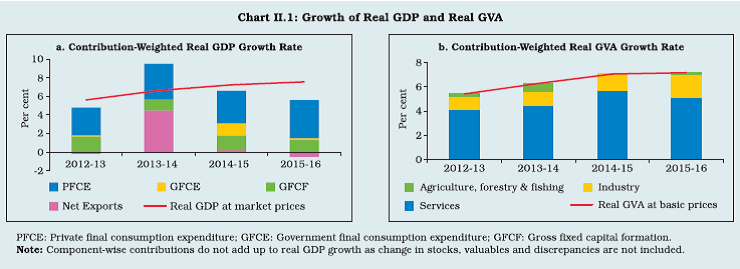 II.1.4 Gross fixed capital formation (GFCF) remained subdued during 2015-16. At the same time, business sentiment improved in response to several initiatives such as ‘Make in India’ and faster clearances of stalled projects, particularly, in respect of non-environmental permissions (Chart II.2). The Project Monitoring Group cleared 168 large projects in 2015-16, involving a year-on-year doubling of the value of investment, with the majority of these projects in the power, roads, coal and petroleum sectors. Although private investment remained muted and risk aversion tightened financial conditions, drivers appear to be coming together to provide a congenial ecosystem for a possible turnaround in the capex cycle. Accordingly, the slackening of the overall rate of investment in 2014-15 – for the third year in succession – could have bottomed out in 2015-16. The continuing improvement in saving by private non-financial corporations and a steady reduction in dis-saving by the general government sector are likely to partially offset the decline in households’ physical saving and the pressure on the resources of public sector financial and non-financial corporations. Preliminary estimates showed that the household net financial saving rate increased to 7.7 per cent of gross national disposable income (GNDI) in 2015-16 from 7.5 per cent in 2014-15 and 7.4 per cent in 2013-14. The improvement reflected a higher rate of increase in gross financial assets in relation to that in financial liabilities. The increase in gross financial assets was driven primarily by a turnaround in small savings and increases in investment in equities and mutual funds, tax-free bonds by public sector units and currency holdings even as the growth in bank deposits held by the households moderated (Table II.1). Financial liabilities also surged reflecting higher borrowings from banks and housing finance companies by the households during the year. 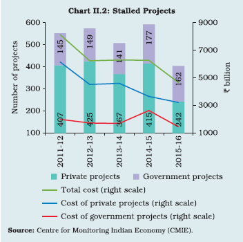
| Table II.1: Financial Saving of the Household Sector | | (Per cent of GNDI) | | Item | 2011-12 | 2012-13 | 2013-14* | 2014-15* | 2015-16* | | 1 | 2 | 3 | 4 | 5 | 6 | | A. Gross financial saving | 10.4 | 10.4 | 10.4 | 10.0 | 10.8 | | Of which: | | | | | | | 1. Currency | 1.2 | 1.1 | 0.9 | 1.1 | 1.4 | | 2. Deposits | 6.0 | 6.0 | 5.8 | 4.9 | 4.7 | | 3. Shares and debentures | 0.2 | 0.2 | 0.4 | 0.4 | 0.7 | | 4. Claims on government | -0.2 | -0.1 | 0.1 | 0.0 | 0.4 | | 5. Insurance funds | 2.2 | 1.8 | 1.6 | 1.9 | 2.0 | | 6. Provident and pension funds | 1.1 | 1.5 | 1.6 | 1.6 | 1.5 | | B. Financial liabilities | 3.2 | 3.2 | 3.0 | 2.5 | 3.0 | | C. Net financial saving (A-B) | 7.2 | 7.2 | 7.4 | 7.5 | 7.7 | *: As per the latest estimates of the Reserve Bank; GNDI : Gross national disposable income.
Note: Figures may not add up to total due to rounding off.
Source: CSO. | Aggregate Supply II.1.5 Real gross value added (GVA) growth at basic prices recorded a marginal pick-up in 2015- 16, held back by the slowing rate of growth in the services sector even as industrial activity accelerated and agriculture and allied activities recovered from the contraction a year ago. II.1.6 GVA from agriculture and allied activities posted a modest growth in 2015-16, in spite of a second consecutive sub-normal monsoon year. The southwest monsoon fell short of normal precipitation levels by 14 per cent on top of the deficiency of 12 per cent in the preceding year’s season, with 17 sub-divisions out of 36 receiving deficient rainfall. The northeast monsoon was also below the long period average (LPA) by 23 per cent with a highly skewed distribution. Weather vagaries in the form of cyclones took their toll towards the close of the season. Reservoir levels were depleted to decadal lows. Notwithstanding these setbacks, the fourth advance estimates of the Ministry of Agriculture have placed foodgrains production for the year at 0.1 per cent higher than in the previous year, mainly due to increase in wheat production. All other major foodgrains as well as commercial crops fell below 2014-15 levels. However, buffer stocks of foodgrains ended the year comfortably above the food stock norms for Q4 due to higher procurement, which also supported higher off-take during the year (Chart II.3). In 2016-17 so far, despite a delayed and tepid beginning, the southwest monsoon has gained momentum since the third week of June, bridging the gaps in precipitation across the agro-climatic regions of the country. As on August 18, 2016, the cumulative rainfall was at its LPA level as against 9 per cent below LPA in the corresponding period of the previous year, leading to an increase of 6.5 per cent in kharif sowing, thus far. 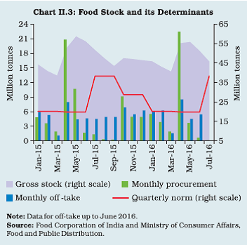 II.1.7 In the industrial sector, value added and its contribution to overall GVA growth surged during 2015-16 (Chart II.1b). In terms of volumes, there was a slowdown from the subdued turnaround in industrial production in the preceding year (Table II.2). While mining accelerated to its highest growth in the past five years, a sharp deceleration in basic metals and contraction in food processing suppressed manufacturing output. The continuing contraction in hydel power constrained a fuller overall expansion in electricity generation. Hamstrung demand from financially stressed DISCOMs operated as a major dampener for plant load factor in respect of thermal power. The disconnect between the largely subdued production and the robust value added for manufacturing reflected the changes in methodology of compilation and data sources of the new GVA series as well as the sharp decline in input costs, shoring up value added and profits. The lacklustre performance of manufacturing continued through the first quarter of 2016-17, dragging overall index of industrial production (IIP) growth lower than that in the corresponding period of the previous year, even as mining and electricity witnessed improvement. Hydel power generation that has been in prolonged contraction mode, however, is expected to pick-up as reservoirs get replenished. II.1.8 In terms of use-based activity, capital goods output contracted during 2015-16, extending a protracted lacklustre performance that set in from 2011-12 except 2014-15. The production of insulated rubber cables turned out to be the main drag in this constituent. Excluding lumpy and order-based insulated rubber cables, which have a miniscule weight in the IIP but suffered an average monthly decline of 85.6 per cent during November-March 2015-16, capital goods output would have risen by 6.0 per cent and the overall IIP by 3.5 per cent. Nonetheless, the depressed production of capital goods, especially machinery, reflects subdued investment demand in the economy. The drag of insulated rubber cables continued beyond 2015-16 into April-June 2016 and is expected to persist for some more time. Excluding insulated rubber cables, IIP growth during April-June 2016 would have been 3.6 per cent, instead of growth of 0.6 per cent. Consumer goods output in 2015-16 came out of contraction in the preceding two years, driven up by durables (mainly gems and jewellery) which offset the decline in consumer non-durables (mainly food products and beverages). The turnaround of consumer goods production was, however, tentative and primarily powered by favourable base effect. Trends in consumer goods production – both for durables and non-durables in April-June 2016 remained broadly unchanged. | Table II.2: Index of Industrial Production | | (Per cent) | | Industry Group | Weight in IIP | Growth Rate | | 2012-13 | 2013-14 | 2014-15 | 2015-16 | April-June | | 2015 | 2016 | | 1 | 2 | 3 | 4 | 5 | 6 | 7 | 8 | | Overall IIP | 100.0 | 1.1 | -0.1 | 2.8 | 2.4 | 3.3 | 0.6 | | Mining | 14.2 | -2.3 | -0.6 | 1.5 | 2.2 | 0.4 | 2.3 | | Manufacturing | 75.5 | 1.3 | -0.8 | 2.3 | 2.0 | 3.7 | -0.7 | | Electricity | 10.3 | 4.0 | 6.1 | 8.4 | 5.7 | 2.3 | 9.0 | | Use-Based | | | | | | | | | Basic goods | 45.7 | 2.5 | 2.1 | 7.0 | 3.6 | 4.7 | 4.8 | | Capital goods | 8.8 | -6.0 | -3.6 | 6.4 | -2.9 | 2.0 | -18.0 | | Intermediate goods | 15.7 | 1.6 | 3.1 | 1.7 | 2.5 | 1.6 | 4.1 | | Consumer goods | 29.8 | 2.4 | -2.8 | -3.4 | 3.0 | 2.5 | 0.6 | | Consumer durables | 8.5 | 2.0 | -12.2 | -12.6 | 11.3 | 3.7 | 7.8 | | Consumer non-durables | 21.3 | 2.8 | 4.8 | 2.8 | -1.8 | 1.7 | -4.1 | | Source: CSO. | II.1.9 GVA in the services sector decelerated across-the-board in 2015-16, with the slowdown concentrated in public administration, defence and other services. Lead/coincident indicators were mostly softer than a year ago. Steel consumption and cement production improved in Q4. As regards transportation activity, freight/ cargo handled by railways, ports and domestic aviation decelerated. On the other hand, domestic air passenger traffic and sales of commercial and passenger vehicles rose strongly and mitigated the downturn in the sub-sector. Communication activity was impacted by slowing net additions to cell phone connections due to the introduction of inter-state number portability. Trade, hotels and restaurants were affected by a deceleration in foreign tourist arrivals. The category of public administration, defence and other services was held down by the ongoing restraint on public expenditure. The performance of services sector indicators during April-June 2016, continues to emit mixed signals with auto sales, port cargo, tourist arrivals and cement production accelerating even as railway freight and steel consumption contracted while the aviation sector decelerated. II.1.10 The favourable impact of the normal monsoon is expected to work in conjunction with the implementation of the seventh pay commission’s recommendations to provide a boost to consumption demand. Keeping in view the provision made by the central government for additional expenditure on account of pay and pension in its budget for 2016-17, its overall impact is estimated at around 30 basis points (bps) in the GVA growth projected by the Reserve Bank for 2016-17. II.2 PRICE SITUATION II.2.1 Inflation, as measured by the consumer price index (CPI), evolved through three phases during 2015-16. In the early months of the year, food price pressures stemming from unseasonal rains and subsequently from a delayed and skewed onset of the southwest monsoon were muted by strong favourable base effects. By July-August, 2015 inflation ebbed to an intra-year low of 3.7 per cent, the lowest since November 2014. In the second phase from September, the base effects dissipated and inflation rose unrelentingly month after month to 5.7 per cent in January 2016, albeit falling below the target of 6 per cent set for that month in the medium-term disinflation glide path (Chart II.4). Prices of pulses – in particular, arhar – emerged as the main driver of this upsurge. In February-March 2016, i.e., in the third phase, vegetable prices declined and surprised on the downside. Favourable tailwinds from corrections in prices of pulses and downward adjustments in fuel prices pulled down headline inflation to 4.8 per cent in March 2016. 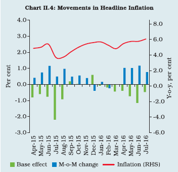 II.2.2 For the year as a whole, inflation averaged 4.9 per cent, down from 5.8 per cent in the preceding year (Appendix Table 4). Sub-group wise, annual average inflation declined across all the major categories, except in the case of fuel and light. The current phase of disinflation in India is driven by a combination of positive developments on the supply side such as fall in global commodity prices and the proactive role played by the government in managing food prices as also the anti-inflationary monetary policy stance of the Reserve Bank (Box II.1). Households’ inflation expectations, which had been persistently elevated, adapted to these developments and current perceptions as well as near-term expectations edged down. Inflation expectations of other agents also mirrored this downshift. Box II.1
Decoding Disinflation Estimated relative contributions of different sub-groups within the consumer price index (CPI) point to significant roles of both favourable supply side factors and the lagged effects of anti-inflationary thrust of monetary policy. A statistical decomposition of contribution of different sub-groups within CPI indicates that the major contribution to disinflation emanated from the food group mainly on account of the government’s astute supply management policies and also from the fall in global food prices (Chart 1). In order to disentangle the roles of demand, supply and policy interventions, a historical decomposition from a vector autoregression (VAR) on CPI inflation, policy rate, crude oil price, output gap and rural wages using quarterly data from 2002:Q4 onwards was attempted. This showed that policy rate changes accounted for about one-fourth of the decline in inflation during April 2014 to December 2015 (Chart 2). Historical decomposition allows identifying the contribution of shocks emanating from each exogenous variable during a specific period in the sample unlike the conventionally used variance decomposition, which explains the forecast error over the whole sample. Slowdown in rural wage growth, supply management policies and the decline in oil prices were other facilitating factors. References: Anand, Rahul, Ding Ding and Volodymyr Tulin (2014). “Food Inflation in India – The Role of Monetary Policy”, IMF Working Paper WP/14/178, September. Rajan, Raghuram (2016). “Policy and Evidence” – speech delivered at the 10th Statistics Day Conference 2016, Reserve Bank of India, Mumbai. II.2.3 During April-July 2016, a sharper than anticipated upturn in the prices of vegetables, sugar, protein-rich items, fruits and pass-through of the increase in global crude oil prices to pump prices of petrol and diesel, reversed the tide. Consequently, inflation recorded a 23-month high at 6.1 per cent in July 2016. II.2.4 Cost conditions were relatively benign during 2015-16, contributing to the disinflationary momentum. Globally, a sizable slack and weak commodity prices kept inflation subdued, with the UK, Japan, Europe and Thailand overcast with deflation risks. In some EMEs even as recession set in (Brazil and Russia), currency depreciation and structural bottlenecks kept inflation elevated (Chart II.5). II.2.5 Crude oil prices treaded softly throughout the year – barring short-lived upticks on incoming data – and dipped to US$ 28 a barrel in January 2016, a 12-year low in terms of the Indian basket of crude oil. Non-energy commodity prices, particularly of metals and agricultural products also remained soft in the presence of spare capacity and weak demand (Chart II.6). These developments depressed input costs in India considerably, especially those relating to raw materials and intermediates. II.2.6 Falling costs, especially on account of declining international commodity prices, kept wholesale price index (WPI) inflation in negative territory for 17 consecutive months up to March 2016. Other indicators of inflation as measured by CPI-IW, CPI-AL, CPI-RL and the GVA deflator also eased during 2015-16. Minimum support price (MSP) increases were much more moderate in 2015-16 than in earlier years. Growth rates of rural wages and employee compensation in the organised sector were modest and the corporate sector reported slower growth in staff costs. Although input prices picked up towards the latter part of the year as polled in purchasing managers’ indices (PMIs) and surveys of business (including the Reserve Bank’s Business Expectations Survey), the weakness in pricing power prevented a complete translation into output price increases. 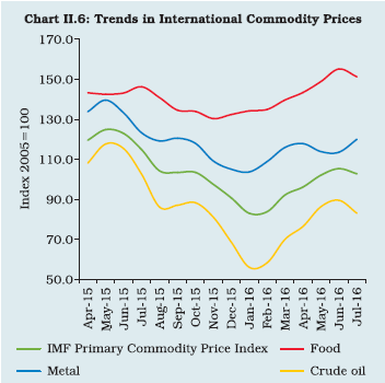
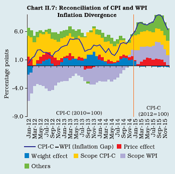 II.2.7 The wide divergence between inflation measured by CPI and WPI was a striking feature of price developments during 2015-16. The divergence in inflation of 7.6 percentage points during 2015 can be explained as the combined impact from: a) difference in prices recorded for similar items (0.9 percentage points); b) difference in weights for similar items (0.03 percentage points); c) difference in inflation for dissimilar items, that is, scope effects (4.9 percentage points); and d) other effects including the differences in the formulae for compilation of these indices (1.8 percentage points)1. The large contribution of scope effects to the overall divergence is unique to 2015 - WPI deflation was concentrated in tradables like basic and intermediate commodities whereas CPI inflation with respect to non-tradables like services, including housing, showed unusual persistence. In a period of rising commodity prices, however, these scope effects tend to cancel out (Chart II.7). 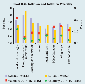 Constituents of Inflation II.2.8 Inflation generally edged down across constituent categories and its volatility was also seen ebbing across the major sub-groups (Chart II.8). While the fuel group was an outlier, the downward inflexibility and persistence in inflation excluding food and fuel, over the greater part of the year was another noteworthy development with implications for inflation dynamics going forward. Food II.2.9 The category comprising food items constitutes 45.9 per cent of CPI and contributed 50 per cent to overall inflation in 2015-16. Within this category, inflation with respect to cereals, fruits and animal-based protein items remained broadly range-bound; pulses and products were the main contributors to food inflation (Chart II.9). Pulses alone contributed 15 per cent to overall inflation during 2015-16 despite a relatively small weight of 2.4 per cent in CPI. Besides the shortfall in production during 2014-15 and the absence of a procurement mechanism until 2015-16, a number of structural factors such as sensitivity to pests and natural calamities kept inflation with respect to pulses at elevated levels. Unseasonal rainfall and temporary supply-demand mismatches pushed up vegetable prices, particularly of onions, during June-September 2015. A number of measures were taken by the government to break the food inflation spiral as part of a comprehensive and rapidly deployed food management strategy – higher MSPs to incentivise production of pulses; procurement of pulses with a view to creating buffer stock; banning exports of most pulses; zero import duty on pulses and onions; raising minimum export prices (MEPs) of onions; and allowing states to impose stock limits for certain essential commodities such as onions, edible oils and pulses. In the case of cereals despite a second successive year of sub-normal monsoon, the prices increased only marginally on account of mild increase in MSPs and higher offtake by the states to check price pressures. 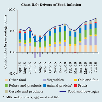 Fuel II.2.10 The fuel group has a weight of 6.8 per cent in the CPI and it accounted for 7.1 per cent of headline inflation during the year. Inflation in this category primarily reflects administered price changes in respect of coal, electricity and LPG as well as other household fuels including firewood and chips. The prices of these items remained sticky during the year. Non-Food Non-Fuel II.2.11 CPI inflation excluding food and fuel edged up gradually through the year and stood at 4.9 per cent in December 2015, before giving ground in the last quarter of the year, and edging lower in July 2016 to 4.6 per cent. These movements were primarily driven by price pressures in the sub-groups of transport and communication, housing, personal care and effects, and health and education (Chart II.10). The cumulative increase of ₹12 per litre and ₹14 per litre, respectively, in petrol and diesel excise duties since November 2014 dampened the pass-through of falling global crude prices into the transport and communication sub group wherein petrol and diesel are embedded. Removing petrol and diesel components of transportation, inflation excluding food and fuel averaged 5.2 per cent in 2015-16, hovering above 5 per cent for the greater part of the year. Housing inflation increased gradually since September 2015. While inflation in personal care and effects edged up a bit in the second half of 2015-16, inflation in services such as health and education exhibited persistent price pressures. Such persistence in price pressures calls for a better understanding of the price-setting behaviour in the economy (Box II.2). 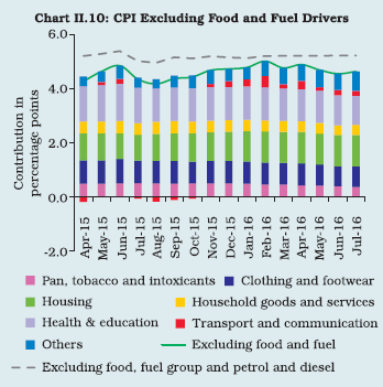 Box II.2
Price Setting Behaviour in India A random effect ordered probit model estimated for the panel of companies covered in the Reserve Bank’s Industrial Outlook Survey from 2010 to 2014 suggests that raw material costs, labour costs (proxied by employment) and the cost of finance influence price setting behaviour with decreasing order of influence. Pricing decisions generally vary based on company size, past price changes and seasonality as well as firms’ adjustments to shocks. The study’s findings show that firms respond more often to a positive price shock by adjusting prices upwards than in the opposite direction. Similarly, strong demand conditions induce a higher increase in prices, whereas the likelihood of lowering prices during weak demand conditions is lower. Using actual retail price data2 for 15 prominent food items over a period of 10 years (2006-15), a measure of price rigidity (constructed as the average number of months in a year when prices either remain unchanged, increase or decline) indicates that the extent of price rigidity varies significantly – while onion prices on an average remained unchanged only in one month during a year, milk prices remained unchanged for about 8-9 months (Chart 1). There is also evidence of price rigidities in protein-rich food items. Reference: Kumari, Shweta and Indrajit Roy (2012), “Price Setting Behaviour of Companies: Evidence from Industrial Outlook Survey”, mimeo. II.2.12 The implementation of the revised pay scales under the seventh pay commission award from August 01, 2016 (with retrospective effect from January 1, 2016) is expected to increase headline inflation with a cumulative impact of 10 basis points by March 2017 over the baseline scenario set out in the bi-monthly monetary policy statement of June 2016 (which excluded the impact of the CPC implementation). This reflects indirect effects stemming from an increase in personal consumption expenditures pushing up aggregate demand. The full impact on CPI inflation, which mainly comes through the direct effects of an increase in house rent allowance when it is effected, will be reflected in a staggered manner over ensuing months. In this regard, the Government has constituted a committee to examine the recommendations of the CPC on allowances. Indirect effects through the expectations channel could also feed back into inflation outcomes. State governments are likely to follow up with revisions of salaries and allowances for their employees. Therefore, most of the inflation impact is likely to spill over into the next financial year. II.3 MONEY AND CREDIT II.3.1 The evolution of monetary and credit conditions during 2015-16 was a study in contrast to the preceding year. Whereas the slow pace of economic growth had restrained monetary and credit aggregates in 2014-15, a growing disconnect from underlying economic activity became evident in 2015-16, especially in the second half of the year. Notwithstanding the lower accretion to net foreign assets than a year ago, reserve money expanded at a faster pace, propelled by unusually high and persisting demand for currency. The growth of money supply (M3), on the other hand, slowed in relation to the preceding year, warranting a careful scrutiny of the impact of currency expansion on the relationship between base money and money supply (details given in para II.3.7). As credit conditions improved with a modest lowering of lending rates, banks rebalanced their loans portfolio in favour of the relatively stress-free personal loans segment. The resulting pick-up in credit growth enabled some re-intermediation by the banking system in the flow of funds to the commercial sector. Reserve Money II.3.2 Reserve money (RM) increased by 13.1 per cent on a y-o-y basis in 2015-16, higher than 11.3 per cent a year ago. The resulting injection of liquidity of ₹2.5 trillion during 2015-16 was sizably higher than that in the preceding year. In 2015-16, in a recurring phenomenon characterising intrayear patterns of RM, about 54 per cent of the whole year’s increase in reserve money took place in March, with the period March 25-31, 2016 accounting for 31 per cent of the annual increase. Various factors drove this build-up including high demand for liquidity from banks as they strove to meet year-end targets, particularly when government balances surged with the last instalment of advance tax collection. On the components side, this spike got reflected in accretion to bankers’ deposits with the Reserve Bank, with banks accumulating excess reserves to the extent of 23 per cent over and above the statutory requirement on March 31, 2016. On the sources side, it showed up in the form of reversible net domestic asset creation which fell back in early April. II.3.3 The expansion in RM in 2015-16 primarily took the form of currency in circulation (CIC) which increased by 14.9 per cent. This acceleration – from 11.3 per cent in the previous year – reflects the interplay of several factors such as jewellers’ strike, festival related demand, elections and the like – that are difficult to disentangle quantitatively with precision – which superimposed themselves on the normal requirements of base money by the economy and vitiated the usual seasonal ebb and flow of currency in the system (Box II.3). On the other hand, the growth of bankers’ deposits with the Reserve Bank moderated to 7.8 per cent, reflecting subdued deposit growth and some evening out of excess reserves by banks. However, the usual stockpiling with the Reserve Bank at the end of March 2016 was observed. From early April, there has been further moderation in these holdings of excess reserves, reflecting greater confidence of banks in their ability to access liquidity under the refinements effected by the Reserve Bank in its liquidity management framework (details in Chapter III). II.3.4 On the sources side, compositional shifts marked the profile of RM expansion in 2015-16. Net foreign assets (NFA), which had been the main driver of RM in the year before, fluctuated widely between accretions during April-October 2015 and depletion during February and early March 2016, reflecting bouts of turbulence in global financial markets that rendered capital flows and asset prices highly volatile. It was only in the latter part of March, that risk aversion abated and capital flows to India resumed, enabling some rebuilding of NFA. In the event, the net increase in NFA through purchases of foreign currency from authorised dealers was of the order of ₹631 billion as against ₹3,431 billion a year ago, accounting for 25 per cent of the RM expansion. Box II.3
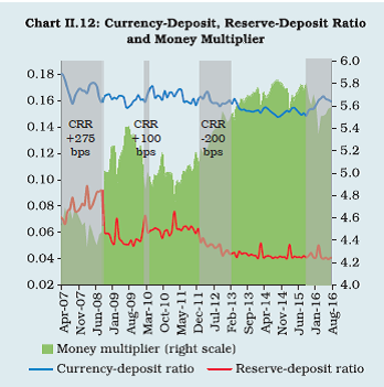
Currency Demand in India Currency demand is governed by several behavioural and institutional factors such as banking habits, sophistication in payment and settlement systems, development of the financial sector, besides the level of income and the opportunity cost of holding currency. The long-run relationship between the demand for currency and its underlying determinants indicates that the income elasticity of currency demand has been more than unity over the period 1989-2011. More recent evidence suggests that the income elasticity of demand for currency is closer to unity. Apart from these fundamental determinants, currency demand is influenced by several frictional factors, e.g., festivals, jewellers’ strike and elections at the union/state levels. The increase in CIC early in the year 2016-17 was also noticeable in states that were not going for elections. Since 2012-13, 26 general elections for state legislative assembly and one for the Lok Sabha have been conducted so far. A surge in currency demand by around 11 per cent on a year-on-year basis in May 2014 across India coincided with the general election. State elections also coincided with large currency demand in those states and/or neighbouring states. The increase in currency in absolute terms during April-May 2014, was around ₹650 billion, ₹268 billion higher than that in April-May 2013. The growth of CIC (y-o-y) and its trend (using Hodrick– Prescott filter) during the election window (Lok Sabha and cluster of states) of 7 months, with election results in the centre of the interval show that there has generally been an upward movement in currency in the election run-up period, which subsides after election results (Chart 1). In order to check the empirical regularity of this phenomenon, a model using monthly data on CIC, lagged CIC to control for persistence in currency demand and election dummies was estimated as under: 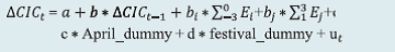 where Ei represents dummy variable for the ith month before election, E0 is the dummy for the election result month and Ej represents a dummy in the jth month after election. The increase in CIC (m-o-m, per cent) was used as a dependent variable. Regression coefficients for months prior to the election were found to be positive and significant, which suggest that CIC increases in the run up to the election. Currency demand in the run-up to elections accounted for close to a fifth of the overall increase in CIC during January- March 2016. CIC is known for its seasonal fluctuations, which picks up in April because of large government expenditure and procurements, and in October/November due to festivals (Dussehra and Diwali). After controlling for these seasonal factors with appropriate dummies, the coefficients of most of the pre-election dummies were found to be positive and statistically significant. Finally, the joint statistical significance of election dummies was evaluated using the Wald Test, which lent credence to these findings. However, post-election month dummies were not found to be statistically significant, though most of them had the expected negative signs. 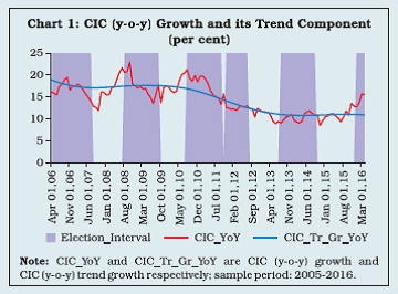 To sum up, the sharp increase in currency demand during 2015-16 may be attributed to a cluster of state elections, apart from other frictional factors such as festival-related demand and jewellers’ strike, even as the underlying relationship between the demand for currency and its fundamental determinants such as income, inflation and interest rates remained stable. Reference: Nachane, D.M., Chakraborty, A.B., Mitra, A.K. and Bordoloi, S. (2013), “Modelling Currency Demand in India: An Empirical Study”, DRG Study No. 39, Reserve Bank of India, February. II.3.5 Net domestic assets (NDA) operations played a stabilising role and also supported the growth of liquidity, constituting around 65 per cent of RM. Within NDA, net RBI credit to the Government increased by ₹605 billion (Chart II.11). Net open market purchases (outright) were around ₹523 billion – comprising net purchases of ₹631 billion through auctions and net sale of ₹108 billion through NDS-OM – as against a net sale of around ₹640 billion a year ago. However, the liquidity impact of these operations was partially offset by increases in cash balances of the Government with the Reserve Bank. Net Reserve Bank credit to banks and the commercial sector, reflecting net repo auctions that injected liquidity into the system to tide over transient episodes of liquidity tightness, increased by around ₹1 trillion during the year to ₹3 trillion as on March 31, 2016 and fell sharply thereafter. The Reserve Bank also transferred a surplus of ₹658.96 billion during the year to the Government, which expanded liquidity as it translated into public spending. II.3.6 In 2016-17 so far (up to August 12), RM grew at 15.0 per cent, far higher than 9.8 per cent in the corresponding period last year, mainly driven by CIC which increased by ₹823 billion as compared with ₹461 billion last year. Another major development has been the OMO (outright) injection of ₹905 billion during the year so far in pursuance of the move to a liquidity position closer to neutrality, as against an OMO sale of ₹223 billion in the comparable period last year, which has reduced the banks’ dependence on the overnight and term windows of the Reserve Bank. Net purchase from authorised dealers, a source of autonomous liquidity has remained relatively muted in 2016-17 so far. Money Supply II.3.7 A break in the organic relationship between RM and M3 became discernible in 2015- 16, beginning from September 2015 right up to August 2016. Driving the unusually high expansion of RM during the year, the acceleration of currency demand to a multi-year high pushed up the currency-deposit (c/d) ratio to a level last observed in May 2012. With the accompanying deceleration in deposit growth, the elevation in the c/d ratio which encapsulates a possible behavioural preference of society for cash vis-à-vis bank deposits, dampened the money multiplier through which RM changes transform into the broader monetary aggregate. This is also corroborated by the upturn observed in the c/d ratio for the household sector since 2014-15. The other determinant of the money multiplier – the reserve-deposit (r/d) ratio – remained broadly stable by contrast, barring the usual end-March spike caused by banks’ overwhelming predilection for balances with the Reserve Bank. This is the first instance in the recent past when the c/d ratio influenced the money multiplier by itself; during April 2007-September 2008, February 2010-April 2010 and January 2012-February 2013, the behaviour of currency demand had either reinforced or offset the impact of changes in the cash reserve ratio (CRR) on the multiplier. These developments pulled down the growth of M3 in 2015-16, especially in the second half of the year, to 10.1 per cent (y-o-y), lower than 10.9 per cent in the previous year (Table II.3). The money multiplier declined to 5.3 in 2015-16 from 5.5 a year ago (Chart II.12). The M3 growth in 2016-17 so far (up to August 05, 2016) at 10.7 per cent remained at the same level as in the previous year. | Table II.3: Monetary Aggregates | | Item | Outstanding as on
August 05, 2016
(₹ billion) | Year-on-year growth (per cent) | | 2014-15 | 2015-16 | 2016-17
(as on August 05) | | 1 | 2 | 3 | 4 | 5 | | I. Reserve Money | 21,772 | 11.3 | 13.1 | 15.0 | | II. Broad Money (M3) | 121,338 | 10.9 | 10.1 | 10.7 | | III. Major Components of M3 | | | | | | 1. Currency with the public | 16,644 | 11.3 | 15.2 | 16.7 | | 2. Aggregate deposits | 104,555 | 10.6 | 9.4 | 9.9 | | IV. Major Sources of M3 | | | | | | 1. Net bank credit to government | 38,063 | -1.2 | 7.7 | 12.8 | | 2. Bank credit to commercial sector | 78,316 | 9.4 | 10.7 | 9.3 | | 3. Net foreign exchange assets of the banking sector | 25,839 | 17.0 | 12.6 | 10.0 | | V. M3 net of FCNR(B) | 118,328 | 11.0 | 10.1 | 10.8 | | M3 Multiplier | 5.6 | | | | Notes: 1. The latest data for Reserve Money pertain to August 12, 2016.
2. Data are provisional. |
 II.3.8 In terms of the components of M3, demand deposit growth broadly tracked the movements in credit. Time deposits were muted by the moderation in deposit rates (both nominal and real), which also reduced the opportunity cost of holding cash. Large issuances of long term tax free bonds by various public sector units contributed to the deceleration in deposits, besides the higher returns on small savings which are not subject to tax deduction at source (TDS). As a result, scheduled commercial banks’ (SCBs’) deposits decelerated to 9.3 per cent in 2015-16, the lowest since 1963-64. The wedge between credit and deposits in terms of growth rates imparted a structural character to liquidity developments during the year. Credit II.3.9 Developments in bank credit during 2015-16 reflected the interplay of several factors. Non-food credit (NFC) growth stalled in the first half of the year, weighed down by subdued off-take and headwinds from asset quality concerns among banks. Beginning November, however, there was a pick-up in credit demand as banks shifted loan portfolio allocations away from the stress-ridden industrial sector and expanded their personal loan exposures, and in particular, housing in which delinquency had been relatively low. Notwithstanding the uncertainty over liquidity coverage ratio (LCR) in January-February 2016 affecting short term rates, NFC growth increased to 10.9 per cent for the year as a whole (10.4 per cent adjusted for UDAY bonds and Bandhan Bank and IDFC Bank, which began reporting data from September and December 2015, respectively), from 9.3 per cent in the preceding year (Chart II.13). 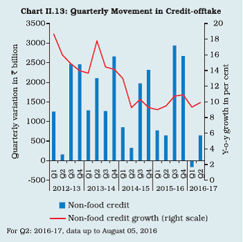 II.3.10 Credit to agriculture, which accounts for 13.5 per cent of NFC, rose by 15.3 per cent, marginally up from 15.0 per cent last year (Table II.4). On the other hand, net flows to the industrial sector slowed markedly to 2.7 per cent – from 5.6 per cent a year ago – reflecting the stress in the larger constituents such as infrastructure, construction, petroleum and coal. Stalling of projects in the power and road segments and dwindling cash flows which affected the quality of bank assets deterred new lending to infrastructure. The credit profile of the construction sector was impacted by the slowdown in real estate and the pressure of unsold house inventories. Basic metal and metal products, chemicals and chemical products, and textiles, on the other hand, absorbed higher credit flows. The credit offtake was also impacted by the high incidence of asset quality stress on balance sheets of banks as well as corporate de-leveraging, especially in Q4. Personal loans turned out to be the strongest driver of bank credit, rising by 19.4 per cent as against 15.5 per cent a year earlier. Within this category, housing loans, which account for more than 50 per cent, went up by 18.8 per cent as against 16.7 per cent a year ago. Credit to the services sector also picked up on the back of higher lending to NBFCs, followed by professional services. | Table II.4: Credit Deployment to Select Sectors | | Sectors | Outstanding as on
June 24, 2016
(₹ billion) | Year-on-year growth (per cent) | | 2014-15 | 2015-16 | 2016-17
(up to June 24, 2016) | | 1 | 2 | 3 | 4 | 5 | | Non-food Credit (1 to 4) | 65,538 | 8.6 | 9.1 | 7.9 | | 1 Agriculture & allied activities | 9,044 | 15.0 | 15.3 | 13.8 | | 2 Industry (micro & small, medium and large) | 26,469 | 5.6 | 2.7 | 0.6 | | (i) Infrastructure | 9,140 | 10.5 | 4.4 | -2.1 | | Of which: | | | | | | (a) Power | 5,288 | 14.5 | 4.0 | -7.7 | | (b) Telecommunications | 910 | 4.2 | -0.7 | 2.0 | | (c) Roads | 1,840 | 6.9 | 5.2 | 9.9 | | (ii) Basic metal & metal product | 4,195 | 6.8 | 7.9 | 9.6 | | (iii) Food processing | 1,460 | 17.3 | -12.5 | -9.3 | | 3 Services | 15,651 | 5.7 | 9.1 | 9.2 | | 4 Personal loans | 14,374 | 15.5 | 19.4 | 18.5 | | Note: Data are provisional and relate to select banks which cover about 95 per cent of total non-food credit extended by all SCBs. | II.3.11 Bank group-wise, public sector banks (PSBs) recorded credit growth of 6.6 per cent during 2015-16 (6.5 per cent in 2014-15) vis-à-vis 24.7 per cent (17.4 per cent in 2014-15) clocked by private sector banks. PSBs witnessed slowdown in credit mainly in respect of industry and infrastructure, i.e., the sectors to which they have large exposure and high incidence of stressed assets. Private sector banks, on the other hand, registered robust credit growth in these segments. In the personal loans segment, both the groups of banks showed higher credit growth during 2015-16, spurred by the lower incidence of stressed assets. II.3.12 NFC growth improved to 9.9 per cent during 2016-17 so far (up to August 05, 2016) from 9.2 per cent in the corresponding period of the previous year. Adjusting for the impact of two new banks and UDAY bonds, NFC growth works out to be 10.4 per cent as on August 05, 2016. Sectoral pattern of credit for June 2016 indicated that personal loans continued to show strong growth, while credit growth to industry remained moderate. II.3.13 The total flow of resources to the commercial sector was far higher by around 14 per cent in 2015-16 than in the preceding year, mainly on account of a pick-up in flows from the banking sources – higher credit disbursal and investment in non-SLR assets (Table II.5). Domestic non-banking fund flows were lower due to the decline in private placements and net issuances of commercial papers (CPs). Initial public offerings (IPOs) picked up in 2015-16 after a lull of around four years. Resource flows from foreign sources were buoyed by the large inflows of foreign direct investment marking an all-time high and compensating for the absolute decline in net disbursements of external commercial borrowings (ECBs). The early months of 2016-17 indicated a slowdown in both bank and non-bank funding for the commercial sector. | Table II.5: Flow of Financial Resources to Commercial Sector | | (₹ billion) | | Sources | April-March | April 01 - August 05 | | 2013-14 | 2014-15 | 2015-16 | 2015-16 | 2016-17 | | 1 | 2 | 3 | 4 | 5 | 6 | | A. Adjusted non-food bank credit | 7,627 | 5,850 | 7,754 | 1,161 | 1,014 | | i) Non-food credit | 7,316 | 5,464 | 7,024 | 999 | 472 | | of which: petroleum and fertiliser credit | 42 | -139 | -18 | -91 | -23^ | | ii) Non-SLR investment by SCBs | 311 | 386 | 731 | 162 | 542 | | B. Flow from non-banks (B1+B2) | 6,505 | 7,005 | 7,052 | 2,521 | 1,859 | | B1. Domestic sources | 4,302 | 4,740 | 4,593 | 1,978 | 1,613 | | 1 Public issues by non-financial entities | 199 | 87 | 378 | 105 | 45# | | 2 Gross private placements by non-financial entities | 1,314 | 1,277 | 1,095 | 333 | 311# | | 3 Net issuance of CPs subscribed to by non-banks | 138 | 558 | 320 | 1,060 | 1,063# | | 4 Net credit by housing finance companies | 737 | 954 | 1,145 | 99 | 153* | | 5 Total accommodation by 4 RBI regulated AIFIs - NABARD, NHB, SIDBI & EXIM Bank | 436 | 417 | 446 | -57 | -35^ | | 6 Systematically important non-deposit taking NBFCs (net of bank credit) | 1,124 | 1,046 | 840 | 376 | 35^ | | 7 LIC's net investment in corporate debt, infrastructure and social sector | 354 | 401 | 369 | 62 | 41^ | | B2. Foreign Sources | 2,203 | 2,265 | 2,459 | 543 | 246 | | 1 External commercial borrowings/FCCB | 661 | 14 | -388 | -11 | -167^ | | 2 ADR/GDR issues excluding banks and financial institutions | 1 | 96 | 0 | - | - | | 3 Short-term credit from abroad | -327 | -4 | -96 | - | - | | 4 Foreign direct investment to India | 1,868 | 2,159 | 2,943 | 554 | 413* | | C. Total flow of resources (A+B) | 14,132 | 12,855 | 14,806 | 3,682 | 2,873 | | Memo: Net resource mobilisation by Mutual Funds through debt (non-Gilt) schemes | 405 | 49 | 147 | 293 | 827 | *: Up to May 2016. ^:Up to June 2016. #: Upto July 2016. -: Not Available.
ADR: American depository receipts; GDR: Global depository receipts; FCCB: Foreign currency convertible bond;
LIC: Life Insurance Corporation of India. | II.4 FINANCIAL MARKETS II.4.1 Global financial markets were roiled by bouts of turbulence during 2015-16 as incoming data renewed concerns about the health of the global economy even as monetary policy stances of systemic economies began to diverge. Domestic markets were impacted by these global cues, although there were differential responses across segments. Equity and foreign exchange markets were most affected by global spillovers and were rendered vulnerable to sporadic overshooting and heightened volatility in response to fluctuations in global financial asset prices and portfolio flows. By contrast, debt markets were shaped more by domestic developments. After yields eased in the first half of the year, they rose in the second half before a generalised moderation set in after the presentation of the Union Budget for 2016- 17. Credit and money markets were relatively sheltered and activity in these segments was driven by domestic factors – asset quality concerns in the former, and the evolution of liquidity in the latter. Money Market II.4.2 Money market activity broadly tracked its usual intra-year pattern in 2015-16. Easy conditions ensued in the beginning of the year – as end-2014-15 balance sheet adjustments unwound – and prevailed right up to the first half of October, interrupted by a brief interlude in the second half of April and in May when liquidity dried up due to a passing slowdown in fiscal spending and again in mid-September due to tax outflows. Money market rates trended below the policy rate with a sustained downside bias, except during mid-April to May. Notably, besides the resumption of public expenditure from June, a structural mismatch between deposit mobilisation and credit off-take during this period engendered surplus liquidity in the money market. The volatility of the weighted average call money rate (WACR) fell significantly. Interest rates in the collateralised borrowing and lending obligation (CBLO) and market repo segments were tightly aligned with the WACR but with a distinct softening tendency. Interest rates on commercial papers (CPs), certificates of deposits (CDs) and 91-day treasury bills also traded on an easing note and priced in 50 bps reduction in the policy rate announced at end-September. Turnover in all segments of the overnight market generally picked up in the first half of the year starting from May 2015. II.4.3 From the second half of October, money market rates, which had dropped by 68 bps in response to the end-September policy rate reduction, began to firm up reflecting the tightening of liquidity on account of slowdown in government expenditure in the run-up to the end-year fiscal targets and increase in currency demand. With deposit growth slipping into single digit along with pick up in NFC, liquidity management was further complicated on account of currency leakage from the banking system on a durable basis (see Box II.3). The WACR firmed up a little above the repo rate, hardening further during the advance tax outflows in mid-December. Other money market rates rose in sync, with spreads relative to the WACR rising to the peak of 28 bps in case of market repo and 29 bps in CBLO in the second half of December 2015. II.4.4 Fiscal rectitude was visible in the general rise in cash balances of the Government throughout the last quarter of the year. Moreover, with the pick-up in NFC during this period, CP and CD rates firmed up and their spread over WACR widened by over 50 bps (Chart II.14). With cash balances of the government and banks being built up to an intra-year peak, the WACR spiked to 10.05 per cent as on March 31, 2016 – a typical end-year phenomenon. Other money market rates also hardened considerably to 7.36 per cent in the CBLO segment and to 7.91 per cent in the market repo segment. Through the second half of the year, turnover in money market segments increased, mainly reflecting the call money and market repo segments, even as the CBLO segment showed a decline. 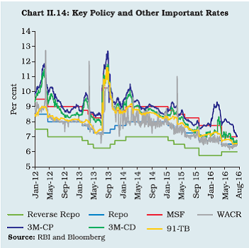 II.4.5 During 2016-17 so far (up to August 11), money market rates have generally exhibited a softening trend on the back of comfortable liquidity situation in the domestic financial system. The WACR remained anchored to the policy rate with a softening bias on account of 25 bps reduction in the policy repo rate in April 2016, narrowing of interest rate corridor to 100 bps, reduction in the minimum daily maintenance of CRR to 90 per cent of the requirement and significant easing of liquidity conditions. The liquidity conditions mostly remained in a surplus mode during July and August 2016 (up to August 11), on the back of pick-up in government spending coupled with the injection of durable liquidity amounting to ₹905 billion by the Reserve Bank through OMO purchases (outright) in consonance with the revised liquidity framework unveiled in April 2016, which envisages lowering the average ex ante liquidity deficit in the system to a position closer to neutrality. Other money market rates, viz., CBLO, market repo, CD and CP rates also softened in sync. G-secs Market II.4.6 In the government securities (g-secs) market, yields hardened in the beginning of 2015 -16 on prevailing bearish sentiments in the market and also tracking a weak rupee. By mid-May, the drying up of liquidity and emergence of stress in the German bund market triggered sell-offs and hardening of yields globally, including in India. Expectations of another sub-normal monsoon also kept yields elevated through June 2015 (Chart II.15). After trading tightly range-bound, yields started to ease from the last week of August as expectations of monetary policy accommodation domestically gained ground, aided by the US Federal Open Market Committee (FOMC) keeping the policy rate on hold in its September meeting. Over the first half of the year, yield moved in a range of 7.53 per cent to 8.09 per cent. Average daily turnover picked up in the secondary g-secs market, up by over 7 per cent from a year ago. From the second week of October, yields firmed up in response to a glut of primary issuances. Expectations of an interest rate hike by the US Fed in December, some increase in inflation and the continuing oversupply of securities due to borrowings by states, concerns on issuance of UDAY bonds, and borrowing by public sector entities through tax-free bonds, also contributed to the firming up of yields. The announcement of the Union Budget 2016-17 including adherence to the fiscal consolidation brought some relief, with the yields easing on a positive sentiment, supported by low inflation during February-March 2016 as well as favourable global developments, particularly the Fed’s dovish guidance. 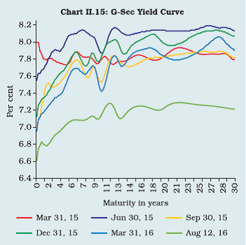 II.4.7 From April to mid-June 2016, the g-secs yields traded range-bound with a marginal hardening bias tracking inflation concerns. Since mid-June 2016, markets have rallied and yields softened on the back of the Brexit referendum, easy liquidity conditions supported by a series of OMO purchases (outright), lower inflation concerns due to normal monsoon so far and expectations of rate cut. The Brexit vote has led to market expectations of easy accommodative stance and low rates by central banks the world over. Further, status quo on interest rate maintained by the US Fed also supported the g-sec yield. As a result, demand for safe haven assets increased and bonds of select EMEs including India rallied on expectations of increased FPI inflows into high yielding bonds. Corporate Debt Market II.4.8 In 2015-16, there was a surge in public issuances of corporate bonds. In the secondary market, however, activity was subdued reflecting low liquidity. Yield spreads over g-secs increased during the year on concerns relating to balance sheet stress and debt servicing capabilities of less than AAA rated corporate issuers (Chart II.16). In the second half of the year, following the September reduction in the policy repo rate and again towards the close of the year, yields of AAA rated corporate bonds eased, following g-secs yields. Foreign portfolio investment in corporate bonds stood at about ₹3.4 trillion at end-March 2016, amounting to around 80 per cent of the limit. Turnover in the corporate bond market declined by 6.3 per cent in relation to the previous year. The corporate bond yields also declined following easing of g-secs yields during 2016-17 so far (up to August 16). Taking advantage of low yields vis-à- vis bank lending rates, corporates raised more resources from the bond market in the recent period. 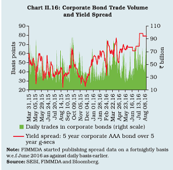 Equity Market II.4.9 The equity market came off the highs scored in 2014-15 and began 2015-16 on a more subdued tone as the slowdown in China followed by the plunge in its equity markets spread bearish sentiment globally. Domestic factors such as mixed corporate performance, deficient monsoon, concerns about the minimum alternate tax (MAT), asset quality in the banking system, sluggish investment activity and depreciation of rupee engendered by portfolio outflows weighed on the market. II.4.10 Market sentiment was boosted by the policy rate cut on September 29, 2015 and supported by signs of improvement in global financial conditions. The indications of additional monetary accommodation by the European Central Bank and the Bank of Japan and of the Fed staying on hold instilled risk-on investor appetite and portfolio flows returned to Indian markets. By the end of October, the tide turned as greater certainty seemed to form around rate action by the Fed in its December meeting. Moreover, weak corporate performance and disappointing domestic cues in the form of inflation rising alongside a loss of momentum in industrial activity kept equity markets weak up to the end of December. The new year (2016) was marked by extreme turbulence in global markets as fears of a China slowdown resurfaced, fanned by the plunge in crude oil prices to a 12-year low. There was an outflow of portfolio investment funds from the emerging economies and India was not immune to this, with associated weakening of the rupee. As public sector banks in India started posting large erosion in profits/losses, a bank led downturn in the equity market took the Sensex down by 17.9 per cent (over end-March 2015) on February 11, 2016, its lowest level since May 2014. The presentation of the Union Budget at the end of February marked a clear turning point. Optimism returned as portfolio flows resumed and the improvement in sentiment provided upside to the rupee. The rally in Asian markets, more generally, aided the rise of the Sensex in March 2016 (Chart II.17). Over 2015-16, the Sensex declined by 9.4 per cent. However, Indian equity markets have shown resilience as compared to other emerging markets. The price to earning (P/E) ratio of MSCI-India was much higher than that of MSCI-EME during this period. 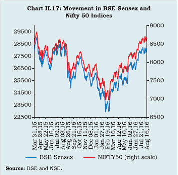 II.4.11 In 2016-17 so far (upto August 18), the Sensex has gained by nearly 11 per cent over end- March 2016 on the back of investor optimism over good progress of monsoon, initiation of reform measures by the government, implementation of the seventh CPC’s recommendations, sustained FPI buying and passage of the GST Bill by the Parliament. Even though the Indian stock market was temporarily affected by Brexit in tandem with sell-off in the global equity markets, it rebounded strongly and pared all its losses in the subsequent sessions. Primary Market Mobilisation II.4.12 The primary segment of the equity market was disconnected from the high turbulence affecting the secondary segment. During 2015- 16, primary resource mobilisation in the form of IPOs surged to its highest level since 2011-12, with 73 IPOs raising resources of the order of ₹143 billion which was four times the mobilisation in the previous year. Resources raised through non-convertible debentures increased by 262 per cent on a year-on-year basis, garnering resources of ₹341 billion. Public sector units (PSUs) raised ₹435 billion through both public issuance and private placement of tax free bonds during 2015-16. Resource mobilisation through IPOs continued to be buoyant and aggregated around ₹75 billion during April-July 2016 as compared with ₹29 billion during the corresponding period of the previous year. Foreign Exchange Market II.4.13 A combination of global and domestic developments impacted the foreign exchange market in the early months of 2015-16. The exchange rate of the rupee traded with a downside bias, and was vulnerable to spillovers from the Greek crisis, global sell-offs, hawkish FOMC guidance and the uncertainty surrounding the evolution of international crude prices. Domestic developments amplified these pressures – the persistent shrinking of exports; portfolio outflows in response to MAT; and projections of a subnormal monsoon. After a brief lull of range-bound movements, the exchange rate came under renewed downward pressure in mid-August with sudden devaluation of the renminbi and the selloffs in Chinese equity markets. The rupee crossed the level of ₹66 against the US dollar at the end of August before stabilising and trading tightly range-bound through September. Through this eventful period for emerging market currencies, the rupee turned out to be better performing among the peer currencies. II.4.14 In the second half of October, depreciating pressures set in again with growing anticipation of policy rate action by the Fed in December. The exit of portfolio investors from Indian debt and equity markets accentuated the pressures on the rupee. Eventually, the increase in the target Federal Funds rate in December turned out to be fully discounted by markets. II.4.15 While the turmoil in international financial markets kept the rupee under pressure through January and the first half of February 2016, conditions stabilised thereafter. The presentation of the Union Budget 2016-17, followed by resumption of portfolio flows on dovish Fed guidance, helped stabilise the rupee and imparted a modest appreciation bias by the close of the year. The depreciation of the rupee against the US dollar during 2015-16 was moderate relative to other EMEs (Table II.6). In nominal terms, it depreciated by 6.6 per cent against the US dollar during the year, while in real effective terms it appreciated by 2.9 per cent against a basket of 36 currencies. Forward premia generally showed a declining trend during 2015-16 reflecting, inter alia, the declining interest rate differential between India and the US. While the interbank segment maintained the previous year’s level in terms of activity, there was a slight dip in merchant turnover. Overall, the spot segment saw an uptick in volumes while forward/swap activity dropped during 2015-16. During 2016-17 so far (up to August 16), the rupee broadly remained range bound with a mild depreciating bias under transient pressure due to Brexit. | Table II.6: Movements in Exchange Rate of Major Currencies in 2015-16 (Based on Average) | | (Per cent) | | Countries | Local Currency
vis-à-vis
US dollar | REER | | 1 | 2 | 3 | | Brazil | -31.0 | -19.3 | | Russia | -29.2 | -14.5 | | South Africa | -19.7 | -8.1 | | Mexico | -17.5 | -12.2 | | Malaysia | -17.2 | -9.3 | | Australia | -15.5 | -8.7 | | Euro Area | -12.4 | -5.8 | | Indonesia | -10.8 | 1.3 | | Japan | -8.4 | -3.1 | | Korea | -8.2 | -1.5 | | Thailand | -7.2 | -1.4 | | Singapore | -7.0 | -1.6 | | UK | -6.4 | 3.0 | | India | -6.6 | 2.9# | | Philippines | -4.2 | 3.5 | | China | -2.6 | 7.5 | | US | 11.7* | 10.2 | #: REER based on 36-currency trade- weighted basket.
*: Based on US dollar Index against the currencies of a large group of major US trading partners;
REER: real effective exchange rate.
Note: (-) represents depreciation of local currency.
Source: BIS, US Federal Reserve Board, Reserve Bank and Reuters. | II.5 GOVERNMENT FINANCES3 II.5.1 The central government achieved the budgetary targets set for 2015-16 through a revenue effort in contrast to preceding years when curtailment of expenditure, often across-the-board rather than targeted, was the main instrument of consolidation. This had positive implications for the quality of central government finances since budgeted capital spending was largely preserved. Further, revenue expenditure declined as a proportion to GDP. The government has reaffirmed its determination to stay the course on consolidation through 2016-17 and bring down the gross fiscal deficit (GFD) to 3.0 per cent of GDP by 2017-18. At the sub-national level, state governments budgeted for a retrenchment in capital outlay in 2015-16 in order to renew their fiscal rectitude after the expansion in capital outlay pushed up GFD in 2014-15. While the return to the path of consolidation is welcome, the potential erosion in the quality of expenditure – the theme of the Reserve Bank’s report on State Finances in 2015-16 – raises concerns. Central Government Finances in 2015-16 II.5.2 The fiscal strategy for 2015-16 was mainly revenue-driven. Additional revenue mobilisation (ARM) accounted for around 15 per cent of indirect tax revenue, imparting significantly higher growth to collections (Chart II.18). Revenue from union excise duty was 23.6 per cent higher than budgeted, reflecting upward duty revisions on petroleum products for consumption-smoothing in the face of a sharp decline in international crude prices. Custom duty collections rose modestly on the back of rate increases, including countervailing and anti-dumping interventions, even as the tax base, i.e., imports shrank. Revenues from service tax rose 25 per cent on account of the revision in the service tax rate from 12.36 per cent to 14.0 per cent during the year and the imposition of the Swachh Bharat cess; also, the negative list (introduced in 2012-13) was pruned, resulting in some increase in the tax base. In contrast, direct tax collections recorded a shortfall of 5.8 per cent relative to budget estimates (BE). Collection of direct and indirect tax revenues in 2015-16 (provisional accounts) was ₹14.57 trillion as against the revised estimate (RE) of ₹14.60 trillion. The total collection thus represents a growth of 17.0 per cent over the previous year. Non-tax revenues exceeded budgetary targets by 16.6 per cent due to higher dividends and profits. Accordingly, notwithstanding the shortfall of 63.6 per cent in the disinvestment target, non-debt receipts turned out to be marginally higher than budgeted. 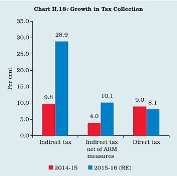 II.5.3 Capital outlay was higher than in 2014- 15, mainly on irrigation, defence and roads and bridges. Apart from the revenue efforts, it was non-plan capital expenditure that bore the brunt of fiscal adjustment. Revenue expenditure grew at a modest rate of 5.5 per cent. II.5.4 Reflecting these developments, the budgeted targets for the GFD-GDP ratio of 3.9 per cent and for the primary deficit (PD) of 0.7 per cent were met as borne out in the revised estimates and provisional accounts. In spite of the shortfall in direct tax revenues, the revenue deficit (RD) at 2.5 per cent was significantly lower than budgeted (2.8 per cent) (Table II.7). | Table II.7: The Central Government’s Fiscal Performance | | (Per cent to GDP) | | Item | 2004-08 | 2008-10 | 2010-15 | 2013-14 | 2014-15 | 2015-16 (RE) | 2015-16 (PA) | 2016-17 (BE) | | 1 | 2 | 3 | 4 | 5 | 6 | 7 | 8 | 9 | | Non-Debt Receipts | 10.4 | 9.5 | 9.5 | 9.4 | 9.2 | 9.2 | 9.1 | 9.6 | | Tax Revenue (Net) | 7.8 | 7.5 | 7.3 | 7.2 | 7.2 | 7.0 | 7.0 | 7.0 | | a) Direct Tax | 5.0 | 5.9 | 5.6 | 5.7 | 5.6 | 5.5 | 5.5 | 5.6 | | b) Indirect Tax | 5.5 | 4.3 | 4.5 | 4.4 | 4.4 | 5.2 | 5.3 | 5.2 | | Non-tax Revenue | 2.1 | 1.8 | 1.8 | 1.8 | 1.6 | 1.9 | 1.8 | 2.1 | | Non-debt Capital Receipts | 0.4 | 0.3 | 0.4 | 0.4 | 0.4 | 0.3 | 0.3 | 0.4 | | Total Expenditure | 13.8 | 15.8 | 14.3 | 13.8 | 13.3 | 13.2 | 13.1 | 13.1 | | Revenue Expenditure | 11.9 | 14.1 | 12.6 | 12.2 | 11.7 | 11.4 | 11.3 | 11.5 | | Capital Expenditure | 1.9 | 1.7 | 1.7 | 1.7 | 1.6 | 1.8 | 1.7 | 1.6 | | Plan Expenditure | 4.0 | 4.8 | 4.3 | 4.0 | 3.7 | 3.5 | 3.5 | 3.7 | | Non-plan Expenditure | 10.2 | 11.0 | 10.0 | 9.8 | 9.6 | 9.6 | 9.6 | 9.5 | | Revenue Deficit | 2.0 | 4.9 | 3.5 | 3.2 | 2.9 | 2.5 | 2.5 | 2.3 | | Gross Fiscal Deficit | 3.4 | 6.2 | 4.8 | 4.5 | 4.1 | 3.9 | 3.9 | 3.5 | BE: Budget Estimates; RE: Revised Estimates; PA: Provisional Accounts.
Note: Direct tax and indirect tax as per cent to GDP do not add up to net tax revenue, which represents tax revenue for the central government net of devolution to the states. | Central Government Finances in 2016-17 II.5.5 Set against the backdrop of the fiscal performance in 2015-16, revenue mobilisation through taxes is likely to lose some buoyancy in 2016-17 – buoyancy of gross tax revenue is budgeted to decline from 2.0 to 1.1. While the growth of gross tax revenue is projected to decelerate over the year, non-tax revenues and disinvestment proceeds have been budgeted to grow sharply during 2016-17. Net receipts from communication services – spectrum auctions, spectrum renewals and licence fees – are budgeted at ₹990 billion while disinvestment proceeds are projected to grow by 123.2 per cent. II.5.6 The central government’s total expenditure is budgeted to pick up in 2016-17 in order to accommodate, inter alia, additional revenue expenditure relating to the implementation of the seventh pay commission and One-Rank-One- Pension (OROP) awards. However, amidst this expansion, capital expenditure – both including and excluding defence – is projected to grow at a considerably slower pace and, in fact, decline as a proportion to GDP. Notwithstanding the deceleration, an allocation of ₹250 billion has been made for recapitalisation of public sector banks (PSBs) under the Indradhanush plan announced in August 2015. Of this amount, the government has already provided ₹229 billion to 13 PSBs in the current fiscal. Among the constituents of revenue expenditure, pensions are set to rise sharply in conjunction with the pay commission award; however, expenditure on major subsidies (food, fertiliser and petroleum) is estimated to fall to 1.5 per cent of GDP from 1.8 per cent a year ago, indicating rationalisation across-the-board. Reflecting these projections, GFD is estimated to fall to 3.5 per cent of GDP in 2016-17 alongside a decline in other key deficit indicators. II.5.7 As per the latest information available, the fiscal position of the central government deteriorated during April-June 2016-17 as compared to the corresponding period of the previous year. RD and GFD, both at their current levels and as per cent of BE, were higher than those in the corresponding period of the previous year. During this period, a substantial increase in tax revenue was offset by the increase in revenue expenditure, particularly plan revenue expenditure. Revenue mobilisation was robust on account of growth in both direct and indirect taxes. Revenue expenditure grew by 24.3 per cent as compared to a growth of 2.4 per cent in the corresponding period of the previous year. Capital expenditure registered a significant decline, both under plan and non-plan heads. II.5.8 As per the seventh pay commission’s recommendations, the total burden for the central government on account of pay, pensions and arrears will amount to ₹606.08 billion in 2016- 17. The central government has provisioned for ₹538.44 billion in Union Budget for this, which suggests a shortfall of ₹67.64 billion (0.04 per cent of GDP)4 for 2016-17. The government will get direct tax revenue from the beneficiaries of higher salaries and pensions as well as indirect taxes on goods and services purchased, which, to a large extent, would have been factored in the budget estimates. State Finances in 2015-16 II.5.9 The partial information available with respect to 26 states5 suggests that the key deficit indicators in 2015-16 (RE) have deteriorated from BE. As against the budgeted GFD-GDP ratio of 2.4 per cent for 2015-16, states’ GFD-GDP ratio increased to 3.3 per cent in 2015-16 (RE) due to deterioration in revenue account, while capital outlay remained stable. The revenue account deteriorated mainly due to decline in both tax and non-tax revenues. State Finances in 2016-17 II.5.10 The GFD-GDP ratio for state governments for 2016-17 is budgeted at 2.8 per cent while the revenue account is expected to turnaround from a deficit to a surplus mode, indicating the states’ intentions to revert to the process of fiscal consolidation (Chart II.19). Improvements in the fiscal position are based on budgeted higher tax revenues and lower development expenditure (Box II.4). Box II.4 Regional Imbalance in Socio-economic Development The impact of growth on socio-economic development has not been uniform across all Indian States. If the indicators of economic growth, installed power capacity and the credit to deposit (C-D) ratio are factored in, only a few states have emerged as leading in terms of both growth and economic development (Table 1). Goa (5.1 per cent), Kerala (7.1 per cent), Himachal Pradesh (8.1 per cent), Sikkim (8.2 per cent) and Punjab (8.3 per cent) registered the lowest poverty rates and performed much better than the all-India average of 21.9 per cent during 2011-12. State-wise data on human development indicators also display considerable variations. Jammu and Kashmir, Assam and Manipur are usually unable to attract sizable private investments due to poor infrastructure which would be difficult to upgrade due to lack of resources. The challenge, in essence, is to break this vicious circle. | Table 1 : Classification of States (2004-05 to 2013-14) | | Indicators | Best Performing States | Average Performing States | Least Performing States | | Economic Growth (CAGR) | (>8.5)
Sikkim, Uttarakhand, Delhi, Goa, Gujarat, Haryana, Maharashtra, Tamil Nadu, Tripura, Bihar, Mizoram | (>6.0 but <8.5)
Andhra Pradesh, Arunachal Pradesh, Chhattisgarh, Himachal Pradesh, Jharkhand, Karnataka, Kerala, Madhya Pradesh, UP, Rajasthan, Punjab, West Bengal, Odisha, Nagaland, Meghalaya | (<6.0)
J&K, Assam, Manipur | | Installed Capacity of Power (CAGR) | (>15.0)
Chhattisgarh | (>7.5 but <15.0)
Delhi, Gujarat, Haryana, Himachal Pradesh, Madhya Pradesh, Maharashtra, Odisha, Sikkim | (<7.5)
Assam, Nagaland, Rajasthan, Karnataka, Tamil Nadu, Uttar Pradesh, Uttarakhand, J&K, Tripura, Andhra Pradesh, West Bengal, Punjab, Bihar, Arunachal Pradesh, Goa, Mizoram, Kerala, Manipur, Meghalaya, Jharkhand | | C-D Ratio (CAGR) | (>4.0)
Nagaland, Punjab, Delhi, Rajasthan, Andhra Pradesh, Sikkim, Kerala, Haryana, Uttarakhand, Arunachal Pradesh, Gujarat, Tripura | (>1.0 but <4.0)
Uttar Pradesh, Chhattisgarh, Jharkhand, Bihar, Tamil Nadu, Maharashtra, West Bengal, Madhya Pradesh, Karnataka | (<1.0)
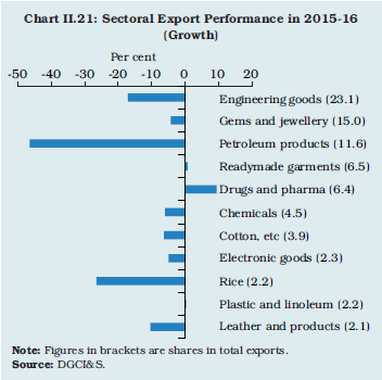
Goa, Assam, Himachal Pradesh, J&K, Manipur, Meghalaya, Mizoram, Odisha | | CAGR: Compound Annual Growth Rate (per cent). | References: Arnold, I. J. and E.B. Vrugt (2002), “Regional Effects of Monetary Policy in the Netherlands”, International Journal of Business and Economics. Kohali, A. (2007), “State and Redistributive Development in India”, Princeton University Press. Cecchetti, S. G. (1999), “Legal Structure, Financial Structure, and the Monetary Policy Transmission Mechanism”, National Bureau of Economic Research, WP No. 7151. Nachane, D. M., P. Ray, and S. Ghosh (2002), “Does Monetary Policy Have Differential State-Level Effects? An Empirical Evaluation”, Economic and Political Weekly. General Government Finances in 2015-16 II.5.11 In view of the deterioration in state finances during 2015-16, the general government gross fiscal deficit increased to 7.2 per cent of GDP from 6.5 per cent in 2014-15. The combined finances of the central and state governments, however, reflect the resolve towards consolidation, with the general government GFD budgeted at 6.3 per cent of GDP for 2016-17. II.6 EXTERNAL SECTOR II.6.1 India faced a testing international environment in 2015-16, as did other EMEs, with still weakening global trade and growth rendering external demand anaemic. The pass-through of soft international commodity prices to import prices was quick albeit uneven while the dent in commodity export prices was more moderate. Consequently, the terms of trade gains that accrued were larger than in the preceding year. Even as the drag from external demand pulled down exports, imports continued to shrink at a faster pace and the trade deficit narrowed to its lowest level since 2010-11. Bouts of volatility because of high turbulence in global financial markets produced misalignments and overshoots in major exchange rates and asset prices. As a result, the Indian economy was exposed to sudden shifts in sentiment on global cues and considerable flux in net capital flows, particularly portfolio flows, which impacted the financial account of India’s balance of payments (BoP)6. Notwithstanding these challenging developments, astute management including a progressively liberal FDI policy ensured a steady improvement in external sector sustainability, with the level of reserves being built up by US$ 17.9 billion on a BoP basis in 2015-16. Merchandise Exports II.6.2 The slump in commodity prices, weak global demand and a surge in protectionist measures across advanced and emerging economies pulled exports into contraction for the second consecutive year in 2015-16 (Chart II.20). Overall, exports declined by 15.5 per cent to US$ 262.3 billion in 2015-16. Further, the decline was pervasive across constituents, with several items shrinking in terms of both volume and value (Chart II.21). Lower oil prices brought refined petroleum exports to about half their level a year ago. Non-oil exports declined by 8.5 per cent, with exports of key products including engineering goods, electronics, leather and gems and jewellery contracting in terms of either volume or value or both. Sector-specific constraints were also manifest: for engineering goods, demand weakened in key markets; for gems and jewellery, declining gold prices interacted with weak demand; and for cotton exports, it was the sharp slowdown in demand from China. In contrast, drugs and pharmaceutical exports benefited from India’s dominant position as a global supplier of generic drugs and were resilient in the face of various regulatory actions initiated by the US. Readymade garments, particularly high-value apparel, expanded their market share in North America and Europe. Various measures were undertaken during the year to boost exports, including expanded coverage of the Merchandise Exports from India Scheme, raising of duty drawback rates for select sectors and re-introduction of the interest stabilisation scheme. Amid global trade uncertainties, however, exports are yet to show a firm recovery which declined in July 2016 after expanding for the first time in 19 months in June. 
 Merchandise Imports II.6.3 Imports contracted by 15.0 per cent to US$ 381.0 billion in 2015-16, primarily due to a sharp reduction in the oil import bill (Chart II.22). With the price of imported crude oil declining by about 45 per cent during the year, petroleum, oil and lubricant (POL) imports fell by about 40 per cent even as volume picked up by 10.6 per cent over the previous year’s level. Gold imports fell by 7.7 per cent, despite import volumes gaining by 5.7 per cent and inching towards the 2011-12 peak. Non-oil non-gold imports recorded a broad-based decline, barring a few items such as machinery, pulses, fertilisers and electronic goods which rose sharply to either bridge the widening domestic supply gaps or in response to a turnaround in sector-specific investments (Chart II.23). Notably, imports of iron and steel rose in volume terms despite the application of customs/ safeguard duties and imposition of floor prices. However, urea imports fell in response to a record domestic production, but other types of fertiliser imports rose in both value and volume terms. The strong revival of domestic coal production reduced imports sizably. Notwithstanding the mild recovery in global crude oil prices and rise in volume of POL imports, the double-digit decline in merchandise imports continued during April-July 2016. 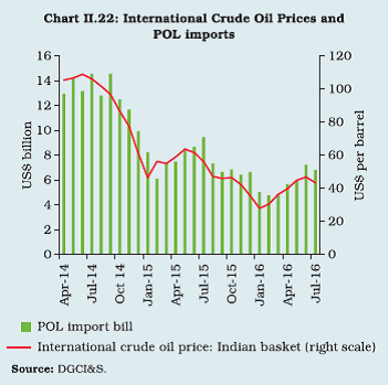
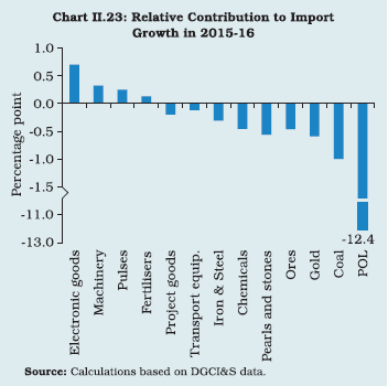 Invisibles II.6.4 Net surpluses from invisibles have traditionally provided support to BoP by offsetting a part of the trade deficit. The difficult international trade environment impacted these invisible transactions diversely in 2015-16. Among services, exports of merchandise trade related transportation services were significantly impacted by the deceleration in global trade and cargo movements. On the other hand, the launching of e-tourist visas in November 2014 and depreciation of the rupee during the year seem to have benefited inbound tourist arrivals and exports of travel services. India’s software exports remained broadly resilient in the face of slow global growth, benefiting from higher demand in banking, financial services and insurance, retail distribution and manufacturing in major destinations such as the US and continental Europe. Among other items of invisibles, remittances inflows weakened in 2015-16 reflecting sluggish activity, particularly in the Gulf region which accounts for more than half of the total remittances received in India (Box II.5). With a rise in both income receipts and payments, the net outgo for income payments remained almost stable in 2015-16. Box II.5 Factors Influencing Remittances to India In India, remittances have financed about 21 per cent of the trade deficit over the last five years. Even though remittances are a relatively durable source of receipts, a number of studies suggest that they are prone to various push and pull factors. Since the Gulf region is a major host of migrants from India, the downtrend in international crude oil prices since the second half of 2014-15 has apparently impacted the momentum in inbound remittance flows. Furthermore, subdued income conditions in other advanced economies in the post-crisis period may also have accentuated the slowdown in remittances inflows to India (Chart 1). 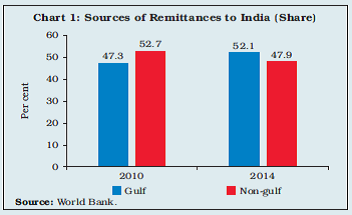 A vector error correction model (VECM), using annual data from 1982 to 2015, shows that the long-run elasticity of remittances with respect to crude oil prices is about 0.7 (Table 1). An increase in per capita income in non-Gulf source countries boosts remittance flows to India. Since the fiscal policy in the Gulf countries is highly dependent on oil revenues, crude prices and public expenditure in these countries are highly correlated (Chart 2). The impact of oil prices on remittances is relatively subdued if not accompanied by a corresponding decline in public expenditure. As expected, a depreciation of the rupee leads to higher remittance flows to India. | Table 1: VECM Estimates of Remittances to India | | | ECT | Cointegrating Equation | DUMEXP | R2 | Adj R2 | | C | LOP | LPEXP | LPCY (-1) | LER | DR | | Eq.1 | -0.61* | -1.96 | 0.71* | | 0.99* | 0.70* | 0.10* | | 0.47 | 0.20 | | Eq.2 | -0.38* | -2.59 | 0.59* | | 1.41* | 0.36* | 0.09* | -0.21* | 0.62 | 0.43 | | Eq.3 | -0.42* | -1.91 | | 0.84* | 0.83* | 0.50* | 0.08* | | 0.57 | 0.38 | LOP: International crude oil price (Dubai fateh);
LPEXP: Public expenditure in Gulf countries;
LPCY: Per capita income of top six non-gulf countries, viz., US, Canada, UK, Singapore, Australia and Italy weighted by their share in India’s total remittances;
LER: Rupee exchange rate vis-à-vis the US dollar (₹/US$);
DR: Domestic interest rate on deposits with 3 to 5 years maturity;
DUMEXP: Dummy as a control variable for years when both crude prices and public expenditure fall;
ECT: Error correction term.
*Significant at 1 or 5 per cent level. |
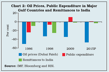 Notwithstanding the sharp decline in oil prices in 2015, the fall in remittances to India has remained modest, offset by other factors such as rupee depreciation, a modest rise in overall public expenditure in gulf countries, growth in per capita income in advanced economies and a favourable interest rate differential. Current Account Deficit II.6.5 Notwithstanding the decline in net invisibles, the sharp fall in the merchandise trade deficit enabled a narrowing of the current account deficit (CAD) from 1.3 per cent of GDP in 2014- 15 to 1.1 per cent in 2015-16, the lowest since 2007-08. It is noteworthy that since 2013-14, CAD has remained well within the limits of external sustainability, aided by fall in gold imports and favourable terms of trade (Chart II.24). External Financing II.6.6 Buoyed by measures to enhance FDI – including raising the ceiling for investments in several important sectors such as broadcasting and defence, as well as rationalising and simplifying procedures and the Make in India initiative – net inflows of FDI surged to US$ 36 billion in 2015- 16, the highest annual net inflow thus far and about 15 per cent higher than in the previous year. Even gross FDI flows to India were at a record high of US$ 55.6 billion during the year. Defying the dominance of mergers and acquisitions in global FDI inflows, green-field investments largely dominated FDI flows to India tripling over the level in 2014 and replacing China as the top destination for green-field FDI (Charts II.25 & II.26). Inflows in the form of deposits by non-resident Indians also remained strong, growing to nearly US$ 16 billion during the year. Net portfolio flows turned negative during the year with estimated net outflows of US$ 3.5 billion from the equity market and US$ 0.5 billion from debt, in line with the experience of other emerging markets. The sell-off across EMEs reflected concerns about interest rates rising in the US and diverging monetary policy stances in other advanced economies, the slowdown in key emerging markets and heightened geo-political tensions. Other debt-creating flows such as ECBs and trade credits also were negative under the weight of repayments which exceeded fresh disbursements (Chart II.27). 
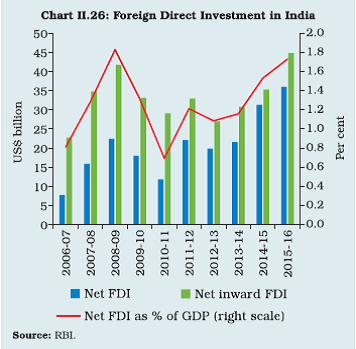
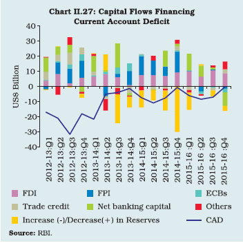 Sustainability II.6.7 External vulnerability indicators improved in 2015-16 as lower CAD and relatively ample net capital inflows enabled a build-up of foreign exchange reserves as buffers against external shocks. By the end of 2015-16, India’s foreign exchange reserves reached a record level of US$ 360.2 billion and improved most of the reserve-based indicators of external vulnerability (Table II.8). Furthermore, FCNR(B) deposits and swaps undertaken under the Special Scheme in 2013 and maturing between September and November 2016 are adequately covered by the Reserve Bank’s forward purchases and are unlikely to pose any serious downward risk to foreign exchange reserves. Going forward, the viability of the external sector outlook will hinge around (i) CAD remaining within sustainable limits; (ii) gains from terms of trade as long as they can be reaped; (iii) a sustained revival of exports, drawing on improvements in competitiveness and productivity rather than a boost from world demand; and (iv) the pace of domestic structural reforms to instil confidence among international investors in India as a preferred investment destination. | Table II.8: External Sector Vulnerability Indicators | | (Per cent) | | Indicator | End-Mar 2013 | End-Mar 2014 | End-Mar 2015 | End-Mar 2016 | | 1 | 2 | 3 | 4 | 5 | | 1. External Debt to GDP Ratio | 22.4 | 23.8 | 23.8 | 23.7 | | 2. Ratio of Short-term to Total Debt (original maturity) | 23.6 | 20.5 | 18.0 | 17.2 | | 3. Ratio of Short-term to Total Debt (residual maturity) | 42.1 | 39.7 | 38.5 | 42.6 | | 4. Ratio of Concessional Debt to Total Debt | 11.1 | 10.4 | 8.8 | 9.0 | | 5. Ratio of Reserves to Total Debt | 71.3 | 68.2 | 71.9 | 74.2 | | 6. Ratio of Short-term Debt to Reserves | 33.1 | 30.1 | 25.0 | 23.1 | | 7. Ratio of Short-term Debt (residual maturity) to Reserves | 59.0 | 58.2 | 53.5 | 57.4 | | 8. Reserves Cover of Imports (in months) | 7.0 | 7.8 | 8.9 | 10.9 | | 9. Debt Service Ratio | 5.9 | 5.9 | 7.6 | 8.8 | | 10. External Debt (US$ bn) | 409.4 | 446.2 | 475.0 | 485.6 | | 11. Net International Investment Position (IIP) (US$ bn)* | -326.7 | -340.8 | -364.6 | -361.5 | | 12. Net IIP/GDP Ratio | -17.8 | -18.2 | -18.3 | -17.7 | | 13. CAD/GDP Ratio | 4.8 | 1.7 | 1.3 | 1.1 | Note:*: (-) sign implies net claims of non-residents on India.
Source: RBI. |
|