There is a greater recognition now than ever before that growth-giving elements of public spending have to be preserved and cultivated. COVID-19 has offered a unique opportunity to redefine fiscal policy in a manner that emphasizes ‘how’ over ‘how much’ by strategic repurposing and reprioritising of public expenditures. In India, institutionalising quality considerations within fiscal management and discipline is the key. This article proposes a few quantifiable indicators, viz., ratios of revenue expenditure to capital outlay and revenue deficit to gross fiscal deficit along with threshold levels for them that can be suitably blended into the fiscal fabric for a sustainable growth trajectory. “Expenditure on physical and social infrastructure including human capital, science and technology is not only welfare-enhancing, it also paves the way for higher growth through their higher multiplier effect and enhancement of both capital and labour productivity. Going forward, it becomes imperative that fiscal road maps are defined not only in terms of quantitative parameters like fiscal balance to GDP ratio or debt to GDP ratio, but also in terms of measurable parameters relating to quality of expenditure, both for the Centre and States, that ....would ensure that welfarism carries significant productive outcomes and multiplier effects” – Shri Shaktikanta Das, Governor, RBI, 2021 Introduction The Covid-19 crisis and the overwhelming fiscal response to drive a recovery from the unprecedented deep contractions in economic activity has necessitated a rethink on the fiscal framework for the future. Increasingly, attention is turning to the quality of public expenditure within the standard approach of setting debt/deficit/expenditure rules to guide fiscal consolidation on the path back to prudence and sustainability. In India, quality considerations remain central to fiscal management and discipline and hence, institutionalising them would entrench these aspects. Typically, fiscal rules aim at correcting distorted incentives and containing pressures to overspend so as to ensure fiscal responsibility and debt sustainability. The cross-country experience reveals, however, that rules set up in terms of headline fiscal balances tend to impart pro-cyclicality to fiscal policy, lower the quality of fiscal spending, and reduce discretion in the hands of the government to respond to exogenous/ uncertain shocks to business cycles (Mandon, 2014; Guerguil et al., 2017). It is in the context of the latter that second-generation fiscal rules have incorporated escape/ buoyancy clauses1 and/or are defined in cyclically adjusted terms (rather than headline fiscal balances) in view of their superior stabilisation properties (IMF, 2014; Schaechter et al., 2012). While such clauses may entail moral hazard and may face communication challenges, expenditure rules have become the preferred option as they are well understood, easy to monitor and reduce the pro-cyclicality of fiscal policy (Manescu and Bova, 2021)2. In this specific vein, a clear lesson for India, from cross-country experience as well as its own historical past, is to not compromise on the quality of public expenditure. The COVID-19 pandemic has brought to the fore the need to spend on merit goods and public goods, in particular those that improve human and social capital and physical infrastructure (IMF, 2020). Prudence too justifies the focus on quality of expenditure. With large scale financing of government expenditure through market borrowings, it is important that borrowed money, which imposes cost and debt servicing pressure, is utilised for productive means with long term returns (Subbarao, 2012; Bhanumurthy et al., 2019). Public expenditure should induce high multiplier capital expenditure and minimise crowding-out risks, particularly when private investment recovery is on the anvil (Alesina and Perotti, 1995; Gupta et al., 2005; RBI, 2019). Also, good quality expenditure that can help relieve critical supply constraints will be non-inflationary. Against this backdrop, the remainder of the article is structured as follows: Section II provides an overview of the cross-country experience with regard to nature of fiscal adjustment from the specific viewpoint of its impact on quality of expenditure and hence, growth. Section III discusses in brief the stylised facts on India’s fiscal experience, both at the centre and states, in terms of various quality of public expenditure parameters, individually and as a composite index, amidst quality features of extant fiscal rules. Section IV deals with the way forward by setting out analytically the critical elements of a post-pandemic fiscal framework for India that blends quantitative dimensions of debt sustainability as traditionally defined with criteria that preserve and enrich the quality of expenditure so as to secure the greatest common good. Concluding policy perspectives are laid down in Section V. II. Quality of Expenditure: Cross-Country Experience Since the mid-1990s, countries across the world have undertaken fiscal consolidation as an integral element of policy frameworks to address macroeconomic and financial instability, recognising that fiscal policy has a key role in eliminating these disequilibria. At the core of the adjustment is a reduction of the fiscal footprint in the economy, guided by a variety of so-called ‘fiscal rules’ that seek to set a trajectory of reduction of either deficits, or debt, or expenditure, or a combination thereof. The country experience, especially against the backdrop of large and persisting imbalances, shows that the size of the adjustment tends to become a self-fulfilling end in itself, whereas the principal objective is to foster sustained economic growth on the bedrock of macroeconomic stability. For the fiscal adjustment to be growth-friendly, it is the way in which it is done that matters, not the magnitude. Some components of government expenditure are more productive than others and complement rather than compete with private expenditure, and some tax changes are more beneficial in their impact on resource allocation than others. More recently, therefore, there is a growing consensus in the literature and in the country experience that fiscal rules can contribute to supporting growth if they reduce uncertainty about debt sustainability and future tax burdens, thus stimulating investment and consumption (IMF, 2012). Accordingly, countries are increasingly changing their focus to prioritise the quality of fiscal adjustment with a view to deriving the maximum benefits in terms of promoting growth. From a practical point of view, the quality of fiscal adjustment is difficult to measure, unlike the quantity of adjustment. The country experience suggests that as a general rule, the prioritisation of certain expenditures within the fiscal envelope and the institution of a growth-promoting tax system that is least distortive with respect to the allocation of saving and investment and minimizes the burden of tax compliance are clearly discernible features of a growth-friendly fiscal adjustment. Virtuous categories of expenditure that need to be preserved within the fiscal adjustment process include spending on education, health and infrastructure that have a high social rate of return and are typically not supplied by the private sector; expenditure on administrative and regulatory services that promote a stable environment for entrepreneurship; social safety nets; and effective and efficient public expenditure management best exemplified by budgetary processes that are transparent, comprehensible and timely. Elements of the tax system that enhance the quality of fiscal adjustment are inter alia a uniform and moderate corporate and personal income tax rate with few – if not none – exemptions; a value added tax, preferably with a single rate and minimal exemptions, as a general sales tax; a customs tariff with as low an average rate as possible and limited dispersion; export taxes only as a proxy for income tax in hard-to-tax sectors; and an efficient tax administration that encourages voluntary compliance, monitoring and discourages evasion and fraud (Mackenzie and Orsmond, 1996). In practice, expenditure reductions have been found to be more effective in achieving durable fiscal consolidation than revenue raising measures (Price, 2010; Alesina, 2010). Durable fiscal adjustments have been associated with permanent reductions in current expenditure (de Rato, 2004; McDermott and Wescott, 1996), with non-interest current expenditure - wage bills, pensions, welfare spending and unemployment benefits - bearing the brunt of the correction: Canada (1994-97); Finland (1998); Germany (2003-05); Netherlands (2004-05); Sweden (1994-98); South Africa (1993-2001); Spain (1996-97); and the United Kingdom (1995-98). The country evidence suggests, however, that sustaining or increasing the share of capital expenditure in total expenditure through the fiscal consolidation raised its chances of success, particularly in countries in Asia, Africa and the Pacific region (Gupta et al., 2005; Cabezon et al., 2015). This is mainly associated with the complementary role that public expenditure in social and physical infrastructure plays in crowding-in private investment, mostly in developing countries (Erden and Holcombe, 2005). Reduction in major current expenditure items such as transfers, subsidies and wages have been found to be politically more difficult than other spending items, including public investment (Hagen and Satrauch, 2001). In other countries – the United States (1994); France (1996-97); Chile (1990-2000); Brazil (1999-2003); Russia (1999-2002); and Nigeria (1994) - fiscal consolidation was led by revenue side measures (Okwuokei, 2014). Adjustments from the revenue side have, in general, been short-lived, as in Brazil during 1999-2003 (Blanco and Herrera, 2006; Alesina and Perotti, 1995; Alesina and Ardanga, 2012). The tax-GDP ratio increased from 29 per cent of GDP in 1998 to 35 per cent in 2004. On the expenditure front, while capital expenditure was almost halved to 0.5 per cent of GDP, but current expenditure remained rigid due to ballooning social security and social assistance benefits, personnel cost, and inter-governmental transfers. The increase in tax burden and compression of public investment hampered future growth prospects. In contrast, the fiscal adjustment adopted by South Africa during 1993-2001 had an expenditure focus, which included reduction in wage bills, subsidies and transfers and an increase in capital expenditure. On the revenue front, there were structural reforms - increase in tax base; elimination of exemptions; lower income tax; and increase in Value Added Tax (VAT). Of the 6.5 percentage points reduction in the overall deficit, spending reductions amounted to 3.5 percentage points and revenue increase amounted to 3 percentage points (Okwuokei, 2014). Given the weak revenue base of Emerging Market Economies (EMEs), revenue adjustment measures have essentially focused on structural reforms to expand the tax base and lower rates, with the spending containment accounting for only one-third of the total adjustment (IMF, 2013). Among the middle-income EMEs, with general government expenditure around 20-40 per cent of GDP, the ratio of current to capital expenditure - an indicator of quality of expenditure – is on the higher side for India than its peers with similar level of expenditure (Chart 1a). Consequently, general government capital expenditure remains low, especially in per capita terms (Chart 1b). Spending on human capital, mostly education and health, has emerged post COVID-19 as a preferred choice for public expenditure. On an international comparison, government expenditure on human capital in India is way behind BRICS and advanced nations (Chart 2). 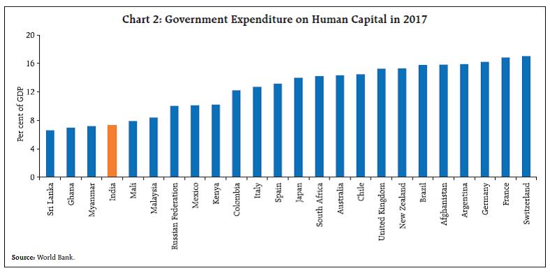 Institutionalising quality of expenditure into fiscal rules is increasingly being found in the EME experience in the post-Global Financial Crisis (GFC) period in a refreshing departure from extant rules that generally target total spending3. Some EMEs have trained focus on quality of expenditure by targeting the recurrent component of spending rather than total spending - viz., Mexico; Peru; Colombia - guided by dual considerations: first, a developmental perspective, which reflects the received wisdom that the composition of public outlays plays a key role in determining its impact on growth (IMF, 2014; Gupta et al., 2005); and second, an effectiveness perspective with evidence supporting better compliance record of expenditure rules than budget balance and debt rules (Cordes et al., 2015)4. III. Stylised Facts in the Indian Experience A turning point in India’s journey along the path of fiscal consolidation was crossed in early 2000s. As an integral element of the macroeconomic adjustment and structural reforms undertaken in the aftermath of the crisis of the early 1990s, India adopted fiscal discipline legislations under the Fiscal Responsibility and Budget Management (FRBM) Act for the centre in 2004-05, which was emulated by a majority of states over the period 2003 to 2008 (Annex I). In the ensuing years, the focus shifted predominantly to adhering to glide paths for the gross fiscal deficit and public debt as proportions to GDP. In the process, however, the quality of expenditure has suffered at both tiers of government, as discussed below. a. The Composition of Expenditure In the standard macroeconomic analysis, the composition of expenditure is employed as a necessary though not sufficient indicator of the quality of expenditure. In essence, it evaluates the resources spent on funding government final consumption expenditure on goods and services for current use vis-à-vis the capital expenditure on goods and services that is intended to create assets that generate future benefits, viz., infrastructure investment in transport (roads, rail and airports), health and research spending5. Historically, dual budgeting, or budgeting separately for current and capital expenditures that originated in European countries in the late 1930s has enabled the differentiation of the productive or more growth friendly types of expenditure from more unproductive ones (IMF, 1995; Afonso et al., 2005). In recent years, the use of a “golden rule” (which allows borrowing only for capital spending), has emerged as a justification for a separate treatment of capital and current expenditures (Premchand, 1989; Jacobs, 2009). In this context, the revenue expenditure to capital expenditure ratio has found appeal in the literature for assessing the optimal composition of expenditure, make cross-country comparisons and assessing the efficacy of policies for switching from revenue to capital to support growth (Devarajan et al., 1996; Forte and Magazzino, 2014; OECD 2020; Bhanumurthy et al., 2019). In practice, this indicator has also seeped into domestic policy analysis on public expenditure to highlight the balancing that needs to be achieved between the different types of expenditure (GoI, 2021; RBI, 2019). The revenue expenditure to capital outlay (RECO) ratio that used to hover at high levels during the 1990s - around 11 for the centre and 9 for states –indicating poor quality of expenditure, saw a significant improvement post-FRBM, which was also associated with high growth in the economy6. These gains were eroded in the post-GFC period (Chart 3a). Correction for large deviations from the glide path of fiscal consolidation often involved cuts in capital outlay. Accordingly, RECO ratio has shown no distinct improvement over the last decade, placed at 7.5 for the centre and at 6.2 for the states in 2019-20 (Chart 3b). b. The Composition of Deficits The share of the revenue deficit in the gross fiscal deficit (RD-GFD) indicates the proportion of borrowed resources exhausted on revenue expenditure rather than investment and, as such, it reflects the quality of expenditure – a lower RD-GFD points to improvement in quality since fiscal multipliers tend to be higher for capital outlays than for current expenditure. Accordingly, it forms part of the forward-looking analysis presented in the Union Budget’s medium-term fiscal policy statement as well as Finance Commission Reports. The FRBM Review Committee Report also envisaged a RD-GFD of about 32 per cent, which would ensure sufficient room for increased capital spending to maximise growth, in line with golden rule of borrowing (GoI, 2017). The RD-GFD has hovered above 70 per cent in the case of the centre, more than twice the level envisaged by the FRBM Review Committee. While the states have fared better, the RD-GFD has been inching up in recent years (Chart 4a and b). 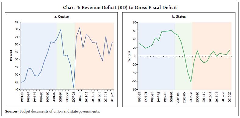 c. Is Expenditure Growth Friendly? Typically, capital outlays are associated with growth giving attributes in view of higher multipliers vis-à-vis other categories, strong employment generation potential and backward and forward linkages with various sectors of the economy (RBI, 2019; Bose and Bhanumurthy, 2013). Accordingly, the proportion of capital outlay in the total spending envelope is used as an indicator of quality, either individually or as one of the components of a comprehensive index with other governance and efficiency parameters (Heriwibobo et al., 2016; IMF, 2014). It is empirically observed that for the European Union (EU) countries the optimal size of public investment is around 10.5 per cent of GDP, whereas the actual public investment prevailed in the range of 4-5 per cent of GDP (Forte and Magazzino, 2014) The institution of FRBM at centre and Fiscal Rule Legislations (FRLs) for states during early 2000s halted the trend decline in capital outlay’s share in total expenditure since 1980-81. The high growth period of 2003-08 was associated with significant rise in share of capital outlay in total expenditure for both centre and states (Chart 5a). The share of capital outlay post- GFC saw a moderation for centre, while a decline for states. Proxying for investment rate, the ratio of capital outlay to GDP has remained stagnant for almost three decades at about 1.5 per cent for centre, while that for states has risen at a moderate pace to about 2.3 per cent, on an average for the post-GFC period, albeit with a decline in last few years (Chart 5b). 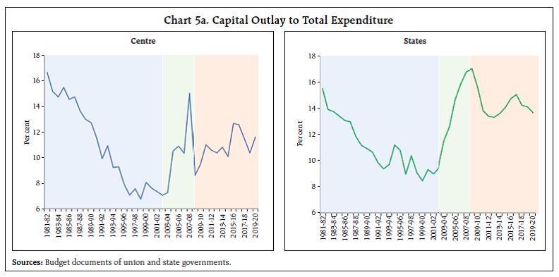 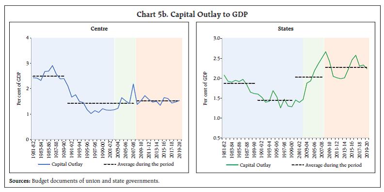 Improving the quality of fiscal expenditure is strongly associated with public infrastructure investments, education and training (together with active labour market policies), health care as well as research and development that support growth by improving the economy’s endowment of production factors (labour and capital) or their productivity (European Commission, 2012). The restructuring of public expenditure towards such productive spending generates a positive effect on growth without creating distortions in the economy that adversely affect growth (Zagler and Durnecker, 2003). The share of committed and uncommitted expenditure to total expenditure is often used as an indicator of quality (Barro, 1990; Gupta et al., 2005; Grigoli, 2012). In the Indian experience, committed expenditure in the form of salaries, pensions and interest payments has first charge on governmental resources. For the centre, committed expenditure remains high and inelastic; for the states, an uptrend is evident in recent years, driven by pensions (Chart 6a and b). The consequence has been that spending on the social and physical infrastructure embodied in developmental expenditure has stagnated over the last two and a half decades, particularly for the centre (Charts 6c and d). d. Financing Pattern As regards financing pattern and composition of expenditure, borrowings for expenditures that are of recurrent nature, and that need to be incurred every year, may not be desirable and should be financed through revenues– the idea underlying the so called ‘golden rule’ in fiscal policy (Zeyneloglu, 2018). Several European nations have also formally integrated this golden rule into their fiscal framework7. This is also linked to the condition for sustainability of budget deficits and public debit (Domar, 1944)8. It may be noted that alongside the deterioration in the indicators of the quality of expenditure observed above, there has been a marked increase in the proportion of market borrowings in financing for both the centre and the states (Chart 7a and b). Increasingly, therefore, resources borrowed at market-based interest rates have gone towards financing revenue expenditure with zero or low returns, against the underlying principle of the golden rule. e. Index of Quality of Government Expenditure Using the six indicators examined above, viz., revenue expenditure to capital outlay ratio; revenue deficit to gross fiscal deficit; capital outlay to total expenditure; capital outlay to GDP; development expenditure to GDP; and committed expenditure to GDP, a composite indicator of quality of expenditure is developed employing principal component analysis (PCA), separately for the centre and for the states9. The indices reveal that there has been a deterioration in the quality of the centre’s expenditure, with some improvements observed during the post FRBM high growth years. In the case of states, the 1990s’ deterioration in quality of spending was not only arrested but also significantly improved during pre-GFC high growth period. The improvement stalled in 2009-10 and there has been a general deterioration in the post-GFC period, although not of the order of the 1990s (Chart 8). 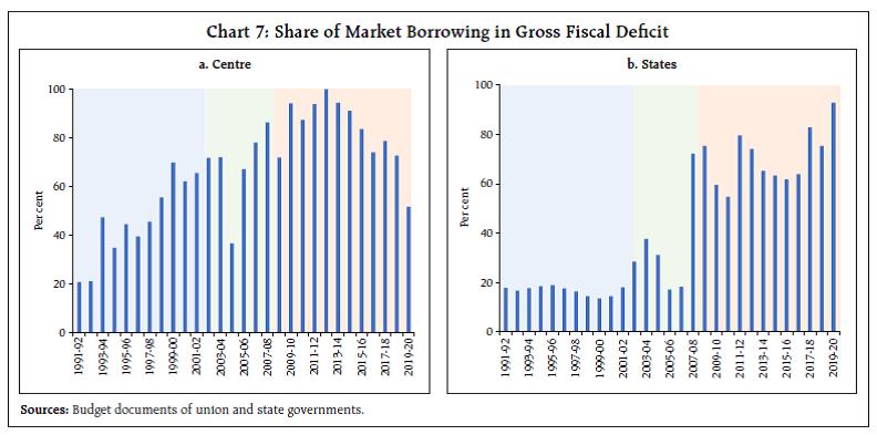 It is noteworthy that fiscal rules, when they were conceived, had embedded features focussing on the quality of expenditure – for instance, the FRBM Act, 2003 sought to build in quality in the form of the prescription of a zero revenue deficit. It has been noted, however, that the emphasis on quality was compromised in the post-GFC period in the overarching pursuit of GFD-GDP targets, with the convergence to a 3 per cent numerical norm being often cited as an aspirational goal (GoI, 2017) (Chart 9)11. Like the centre, states’ FRLs focus on quality through elimination of revenue deficits, maintenance of revenue surplus (Arunachal Pradesh, Manipur, Nagaland, Punjab, Sikkim, Tripura and Uttarakhand) or by linking the revenue deficit to revenue receipts (Tamil Nadu), were broadly achieved except in the post-GFC period. IV. The Way Forward The current stance of the fiscal policy is counter-pandemic, with the general government gross fiscal deficit at around 13 per cent of GDP in 2020-21 and estimated at about 10 per cent in 2021-22. Going forward, a graduated path of withdrawal from pandemic mode is envisaged (Chart 10). A successful normalisation of the fiscal stance is conditional upon an improvement in underlying economic activity. The imperatives of large scale post-pandemic reconstruction warrant that fiscal rectitude should not be achieved at the cost of the quality of expenditure. The thrust of fiscal policy stance on capital expenditure and infrastructure creation, by both centre and states marks the definite intent of the government to improve the quality of expenditure. Accordingly, it may be important to lay down a medium-term fiscal framework with concrete measures and targets (IMF, 2021). Shoring up the quality of expenditure through a quantifiable matrix will help provide the necessary checks and balances and should be integrated into the fiscal framework (Das, 2021). Instead of across-the-board expenditure cuts, a well-thought-out strategic policy mix should protect programmes with high marginal social benefit, thus ensuring that the intent to improve quality fructifies into desirable outcomes. 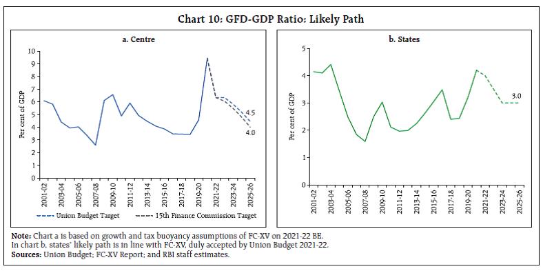 Easier said than done! What should be the design of such a matrix? While it may be difficult to lay down strict quality norms which hold for all tiers of government at all times, an array of indicators could serve as tentative benchmarks. First, an indicative benchmark could be a reduction in the RD-GFD ratio towards levels prescribed by the FRBM Review Committee (GoI, 2017) for the centre, from the current high levels, on the grounds that a major chunk of borrowed money must go towards funding capital expenditure. Second, the endeavour could be to attain a revenue expenditure to capital outlay (RECO) ratio in the range of 4 to 5 which is most growth friendly12. Empirical evidence on thresholds at the general government level for these two indicators – RD-GFD and RECO – also support these ranges (Box I). A third threshold could be through a floor to the capital outlay-GDP ratio or targeting a particular rate of growth in capital outlay so as to arrest the moderation in its share in total expenditure. A large body of theoretical and empirical literature has found a positive relationship between public capital expenditure and growth operating through the crowding-in channel of private investment. The capital expenditure multiplier is also known to be higher than 2 in India (RBI, 2019; Jain and Kumar, 2013). The floor on the capital outlay to GDP ratio should be simple, transparent and well understood13,14. Simulating the announced GFD-GDP target of 4.5 per cent by 2025-26 while maintaining the quality of expenditure through such a matrix will be contingent upon the will to improve the composition of public expenditure (Chart 11). Institutionalising these quality considerations can be the best vaccine for sustainable growth post COVID19. Box I: Quality of Expenditure – Threshold Estimates for General Government in India What is the appropriate mix between revenue expenditure and capital expenditure that can achieve maximum growth?15 An attempt is made to find a link between general governments’ quality of expenditure indicators and economic growth. The ratio of revenue expenditure to capital expenditure indicates a trade-off between the short-term and the long-term. The impact of revenue expenditure on growth lasts for about a year, while that of capex is stronger and longer, with a peak effect after two-three years. An examination of the link between 5-year forward moving average growth in real per-capita gross domestic product (PCGDPG) and the ratio of revenue expenditure to capital outlay (RECO) for the general government (centre plus states)16 in India in an OLS regression framework with suitable controls17 and different threshold levels for RECO ratio (from 4.0 per cent to 5.5 per cent), shows that the positive and significant impact is particularly visible at a threshold of 4.0 to 5.0 beyond which it loses significance. Replacing RECO with another important indicator of quality, as witnessed in previous section, the ratio of revenue deficit to gross fiscal deficit (RD-GFD)18 with all other specifications being the same, a threshold between 30 to 40 becomes significant statistically (Table 1). To sum up, governments at all tiers need to engage in constructive expenditure switching and reprioritisation strategies that shift emphasis from current towards capital spending in order to enhance the impact of fiscal policy on the quality of growth. Borrowings need to be utilised primarily for capital expenditure. | Table 1: Ordinary Least-Square Results | | Dependent Variable: Five-year Forward Moving Average Real Per-capita GDP Growth | | Variables | Eqn. 1 | Eqn. 2 | Eqn. 3 | Eqn.4 | Eqn. 5 | Eqn. 6 | Eqn. 7 | Eqn. 8 | Eqn. 9 | Eqn. 10 | Eqn. 11 | | PCGDPG (-1) | 0.58*** | 0.57*** | 0.53*** | 0.56*** | 0.62*** | 0.46*** | 0.54*** | 0.57*** | 0.59*** | 0.58*** | 0.58*** | | TRDGDP | -0.01 | -0.01 | -0.01 | -0.01 | -0.01 | -0.02 | -0.01 | -0.01 | -0.01 | -0.01 | 0.00 | | RECO | 0.10* | | | | | | | | | | | | RECO (>4.0) | | 0.08* | | | | | | | | | | | RECO (>4.5) | | | 0.07** | | | | | | | | | | RECO (>5.0) | | | | 0.05 | | | | | | | | | RECO (>5.5) | | | | | 0.03 | | | | | | | | RD-GFD | | | | | | | 0.01*** | | | | | | RD-GFD (>30.0) | | | | | | | | 0.01** | | | | | RD-GFD (>40.0) | | | | | | | | | 0.01** | | | | RD-GFD (>50.0) | | | | | | | | | | 0.01 | | | ALR | 0.06** | 0.06** | 0.06** | 0.05** | 0.05** | 0.06** | 0.06** | 0.05** | 0.05** | 0.06** | 0.04* | | TEGDP | -0.01 | -0.02 | 0.04 | -0.02 | -0.01 | 0.04 | -0.05 | -0.03 | -0.01 | -0.04 | -0.04 | | Constant | -1.33 | -081 | -0.30 | -0.40 | -0.73 | -1.19 | 0.08 | -0.27 | -0.78 | -0.07 | 0.46 | | Adjusted R^2 | 0.82 | 0.82 | 0.84 | 0.84 | 0.81 | 0.85 | 0.84 | 0.83 | 0.83 | 0.82 | 0.80 | | LM Test for Serial Correlation | 0.83 | 0.82 | 0.68 | 0.69 | 0.83 | 0.88 | 0.81 | 0.66 | 0.40 | 0.74 | 0.26 | | Heteroskedasticity Test: Breusch-Pagan-Godfrey | 0.93 | 0.94 | 0.89 | 0.71 | 0.90 | 0.99 | 0.89 | 0.95 | 0.99 | 0.91 | 0.70 | Source: RBI staff estimates.
PCGDPG: five-year forward moving average real per-capita GDP growth; TRDGDP: international trade size measured by export plus import as a per cent of GDP; RECO: ratio of revenue expenditure to capital outlay as a proxy of quality expenditure; ALR: adult literacy rate; and TEGDP: total expenditure to GDP ratio to control for size effect of governments' spending.
N.B: (1) Though variables are non-stationary, their residual is stationary indicating cointegrating relationship and thus, OLS can be run.
(2) To identify threshold in RECO, we have used 4 interactive dummy variables where '>' means values more than the threshold, other-wise zero.
(3) ***, ** and * indicate significance at 1,5 and 10 per cent level respectively. | | Debt Considerations The marriage of proposed quality considerations with the GFD-GDP target in this future fiscal paradigm will strengthen the foundation of fiscal consolidation and may entail quantifiable targets for public debt as well. Today, India’s general government debt is at its historical peak of over 90 per cent of GDP. While this is in line with the unprecedented post-COVID rise in debt worldwide, providing a clearly communicated glide path will help reinstate credibility to the fiscal framework. Additional debt can generate returns so as to reduce future debt by strengthening growth and weakening the stock (r-g) and flow (lower primary deficits to GDP) constraints of debt dynamics20. Business Cycle and Measurability Considerations While ‘escape’ and ‘buoyancy’ clauses - which are integral elements of the revised FRBM - may provide the desired and proven flexibility that could make fiscal policy counter-cyclical21, the focus on quality of expenditure along with headline GFD rule is likely to further reduce the element of pro-cyclicality in fiscal policy by making India’s fiscal policy growth friendly with a quality rather than quantity centric expenditure programme22. Comprehensive measurement of GFD by including all off-budget liabilities, as started from this year’s Union Budget, should be maintained to ensure the quality of compliance, leaving no scope for any fiscal rule to be circumvented. Setting up of independent evaluation agencies can help improve fiscal outcomes by ensuring compliance with the targets and improving the quality of adjustments while mitigating the communication challenges associated with adoption of such fiscal frameworks (Eyraud et al., 2018; IMF, 2017). V. Concluding Observations Even as COVID-19 engulfs the world in its deadly grip, leaving a trail of death and destruction in its wake, a renewed interest has been generated in the role of fiscal policy in pandemic times and in life beyond. Increasingly, the narrative is shifting out of the narrow confines of stimulus and consolidation thereafter to an enduring growth-friendly fiscal policy. By strategic repurposing and reprioritising both revenues and expenditures, fiscal authorities have shown that they can extract ‘bang for the buck’ by (a) the public sector leading the private sector into unlocking growth opportunities; (b) the public sector co-existing with the private sector in entrepreneurial partnership; and (c) the public sector stepping back to allow private enterprise to take the lead in sunrise areas, coalescing into an across-the-board improvement in the quality of fiscal spend and eventually in the quality of growth. The Union Budget 2021-22 takes a step in this direction by attempting to reshape the composition of spending in favour of infrastructure, which is appropriate from the point of view of India’s requirement of investment of US$ 1 trillion in the quest for a world class physical infrastructure. This article is an attempt to track this paradigm shift by proposing quantifiable metrics for the quality of public expenditure, which also encompasses upgradation of the social infrastructure by investing in health, education and skilling. If the slant towards emphasis on quality over quantity in the conduct of fiscal policy can be institutionalised into a way of life, the silent revolution will be complete. In essence, this article makes a case for formally incorporating a RD-GFD and a RECO ceiling. As regards the composition of expenditure, RECO ratio of not more than 5 and RD-GFD ratio of not more than 40 per cent for the general government (centre plus states) is empirically found to be appropriate for a sustainable growth trajectory. Apart from satisfying the ‘simplicity’ and ‘easily communicable’ norms of best practice expenditure rules, the formal weaving of quality targets into fiscal consolidation paths will result in setting fiscal policy with a human face, and may even counterbalance the pro-cyclicality bias of fiscal policy by assuring a steady level of provision of public goods of quality. There is a greater recognition now than ever before that in the drive to fiscal rectitude that inevitably follows a period of stimulus, growth-giving elements of the public spending have to be preserved and cultivated. While COVID-19 has tested the limits of flexibility in fiscal policy frameworks in India as in the rest of the world, it has offered a unique opportunity to redefine fiscal policy in a manner that emphasizes ‘how’ over ‘how much’. References Afonso, A.; Schuknecht, L. and Tanzi, V. (2005). Public Sector Efficiency: An International Comparison. Public choice, 123(3), 321-347. Alesina, A.F. (2010). Fiscal Adjustments: Lessons from Recent History. Ecofin Meeting Madrid, April. Alesina, A.F. and Ardanga, S. (2012). The Design of Fiscal Adjustments. Working Paper No. 18423. National Bureau of Economic Research, September. Alesina, A.F. and Perotti, R. (1995). Fiscal Expansions and Fiscal Adjustments in OECD Countries. Working Paper No. 5214. National Bureau of Economic Research, August. Barro, R.J. (1990). Government Spending in a Simple Model of Endogenous Growth. Journal of Political Economy 98(S5): 103-125. Bhanumurthy N.R., Bose, S. and Satija, S. (2019). Fiscal Policy, Devolution and Indian Economy. National Institute of Public Finance and Policy Working Paper No. 287, December. Blanco, F. and Herrera, S. (2006). The Quality of Fiscal Adjustment and the Long-Run Growth Impact of Fiscal Policy in Brazil. World Bank Policy Research Working Paper 4004, September. Bose, S. and Bhanumurthy, N.R. (2013). Fiscal Multipliers for India, National Institute of Public Finance and Policy Working Paper No. 2013-125, September. Cabezon, E., Tumbarello, P., and Wu, Y. (2015). Strengthening Fiscal Frameworks and Improving the Spending Mix in Small States. Working Paper WP15/124. International Monetary Fund. Cordes, T.; Kinda, T. Muthoora, P; Weber, A. (2015) Expenditure Rules: Effective Tools for Sound Fiscal Policy? Working Paper WP/15/29, International Monetary Fund. Das, S (2021), Towards a Stable Financial System. Nani Palkhivala lecture delivered by Governor, RBI, January 21. de Rato, R. (2004). Benefits of Fiscal Consolidation. Remarks to the Real Academia de Doctores, Spain. November Devarajan, S.; Swaroop, V. and Zou, H. (1996). The Composition of Public Expenditure and Economic Growth. Journal of Monetary Economics, Volume 7, Issue 2, April. Diamond, J. (1989). Government Expenditure and Economic Growth: An Empirical Investigation. Working Paper WP/89/45. International Monetary Fund. Domar, E. D. (1944). The Burden of Debt and the National Income. American Economic Review, 34(4): 798–827. Erden, L. and Holcombe, R. (2005). The Effects of Public Investment on Private Investment in Developing Economies. Public Finance Review vol. 33, issue 5. Eyraud, L.; Debrun, X.; Hodge, A.; Lledo, V.; Pattillo, C. (2018). Second-Generation Fiscal Rules: Balancing Simplicity, Flexibility, and Enforceability. IMF Staff Discussion Note, April. European Commission (2012). The Quality of Public Expenditures in the EU. Occasional Paper, 125, December. Forte, F. and Magazzino, C. (2014). Optimal Size of Governments and the Optimal Ratio between Current and Capital Expenditure. Ch 15 in Handbook of Alternative Theories of Public Economics, Edward Elgar Publishing. GoI (2017). Responsible Growth: A Debt and Fiscal Framework for 21st century India. FRBM Review Committee Report (Chairman: Shri N.K. Singh), 1, January. GoI (2021) Fifteenth Finance Commission Report, Government of India. Grigoli, F. (2012). Public Expenditure in the Slovak Republic: Composition and Technical Efficiency. IMF Working Paper WP/12/173. Guerguil, M., Mandon, P., and Tapsoba, R. (2017). Flexible fiscal rules and countercyclical fiscal policy. Journal of Macroeconomics, 52, 189-220. Gupta, S.; Clements, B.; Baldacci, E. and Mulas- Grandos, C. (2005). Fiscal policy, expenditure composition, and growth in low-income countries. Journal of International Money and Finance. Volume 24, Issue 3, April. Hagen, H. V. and Satrauch, R. R. (2001). Fiscal Consolidations: Quality, Economic Conditions, and Success. Public Choice, 109 (3/4), 327-346. Heriwibowo D.; Juanda, B.; Hadi, S.; and Supono, S. (2016). The Measurement of Local Government Spending Quality with Indicators of Sustainable Local Development in Indonesia. Journal of Economics and Sustainable Development ISSN 2222-1700 (Paper) ISSN 2222-2855 (Online), Vol.7, No.4. IMF (1995); Guidelines for Fiscal Adjustment. Fiscal Affairs Department, International Monetary Fund IMF (2012); Fiscal Monitor, International Monetary Fund, October. IMF (2013; 2014; 2017, 2020; 2021). Fiscal Monitor, International Monetary Fund, April Jacobs, D.F. (2009). Capital Expenditures and the Budget. Public Financial Management Technical Guidance Note. International Monetary Fund. Jain, R. and Kumar, P. (2013). Size of Government Expenditure Multipliers in India: A Structural VAR Analysis, RBI Working Paper 07 / 2013, September. Lledo, V.; Yoon, S.; Fang, X.; Mbaye, S. and Kim, Y. (2017). Fiscal Rules at a Glance. International Monetary Fund. Mackenzie, G.A. and Orsmond, W.H. (1996). The Quality of Fiscal Adjustment and Growth. Finance & Development, Volume 0033, Issue 002, International Monetary Fund, June. McDermott, C.J. and Wescott, R.F. (1996). An Empirical Analysis of Fiscal Adjustments. IMF Staff Papers, Vol. 43, No. 4, December. Mandon, P. (2014). Evaluating Treatment Effect and Causal Effect of Fiscal Rules on Procyclicality New assessments on old debate: rules vs. discretion. Working Papers 201414, CERDI. Manescu, C.B. and Bova, E. (2021). Effectiveness of national expenditure rules: Evidence from EU member states. VOX, CEPR Policy Portal. OECD (2020). Government Support and the COVID-19 Pandemic. April Okwuokei, J.C. (2014). Fiscal Consolidation: Country Experiences and Lessons from the Empirical Literature. Chapter 5 in Caribbean Renewal: Tackling Fiscal and Debt Challenges / edited by Charles, Amo-Yartey and Therese Turner-Jones. International Monetary Fund. Premchand, A. (1989). Government Budgeting and Expenditure Controls Theory and Practice. International Monetary Fund. Price, R. (2010). The Political Economy of Fiscal Consolidation. OECD Economics Department Working Papers, No. 776, OECD Publishing, Paris. RBI (2016). State Finances: A Study of Budgets of 2015- 16, Reserve Bank of India, April. RBI (2019). Monetary Policy Report, Reserve Bank of India, April. Schaechter, A., Kinda, T., Budina, N., and Weber, A. (2012). Fiscal Rules in Response to the Crisis: Toward the ‘Next-Generation’ Rules: A New Dataset. IMF Working Papers, 12/187. Subbarao D (2012). “Price Stability, Financial Stability and Sovereign Debt Sustainability Policy Challenges from the New Trilemma”, speech delivered at second International Research Conference, February. Zagler, M. and Durnecker, G. (2003). Fiscal Policy and Economic Growth. Journal of Economic Surveys, Vol. 17, No. 3. Zeyneloglu, I. (2018). Fiscal Policy Effectiveness and the Golden Rule of Public Finance. Central Bank Review, Research and Monetary Policy Department, Central Bank of the Republic of Turkey, vol. 18(3)
Annex I: India’s Fiscal Rules: Centre and States India graduated from its pre-1990 large-scale deficit financing era to the discipline of market-based financing along with fiscal rules under the Fiscal Responsibility and Budget management (FRBM) Act since 2004-05. In order to mitigate the known fiscal risks, a balanced budget rule was introduced, setting a target for gross fiscal deficit (GFD) at 3 per cent of GDP for the central government. While the fiscal discipline achieved in the immediate post-FRBM period was noteworthy, the process was stalled with the global financial crisis (GFC) requiring significant fiscal response on the part of the government. The FRBM kept getting amended repeatedly since 2013-14. A need was felt to bring in desired flexibility by looking at fiscal deficits, after suitably accounting for the business cycles (RBI, 2012; GoI, 2017). To bring in the desired counter-cyclicality, the revised FRBM as adopted in the Union Budget 2018-19 added the ‘escape’ and ‘buoyancy’ clauses23, keeping the adoption of cyclically adjusted budget balance rule in the agenda for the next revision. Also, in line with the evolving global fiscal thinking, threshold level of debt was added as a medium-term anchor in the 2018-19 amendment. Although these were progressive developments, their performance could not be established as envisaged over successive years because of the transition to GST that affected the revenues, the cyclical slowdown of 2019-20 and then the pandemic impact on 2020. Steps towards enhancing transparency also contributed to the deviation of the GFD ratio from the target, with the provisional accounts for 2020-21 placed at 9.2 per cent of GDP for the centre (Chart I.1). 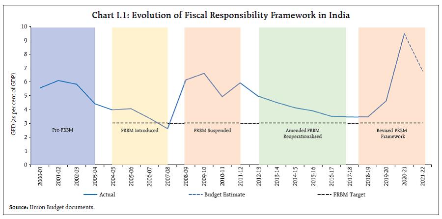 As regards states, there are wide variations in terms of both timeline and target of Fiscal Responsibility Legislations (FRLs). Whereas some southern states (Kerala, Tamil Nadu and Karnataka), Uttar Pradesh and Punjab adopted FRLs before centre’s FRBM Act (2003), most of the remaining states adopted their respective FRLs between 2003 and 2008. West Bengal and Sikkim are the only two states which adopted FRLs after the GFC. Majority of the states target GFD-GDP ratio of 3 per cent along with a deadline to achieve the same. While state FRLs have not seen significant amendments over the years, it may be noted that large scale variations have persisted even in the original FRLs with instances of debt rules in some of them and provisions for escape clauses in others (Chart I.2).
Annex II: Expenditure Rule across Nations Expenditure rules (ER) are a new set of preferred rules that bring in the desired flexibility while being more transparent and easier to monitor, as the expenditure aggregates can be more easily understood than, for instance, cyclically adjusted fiscal balance. Public expenditure tends to move in tandem with revenues, i.e., rising and falling with revenue windfalls and shortfalls, respectively. By keeping a check on spending during good times, ERs can help create some buffers, which may be used to provide a counter-cyclical fiscal push during slowdown (Manescu and Bova, 2021). The ERs set limits on spending in either absolute terms, growth rates or as a proportion of GDP. While extant expenditure rules generally target total spending, some EMEs focus on quality of expenditure by targeting the recurrent component of spending, rather than total spending. As per the Fiscal Rules Database, 45 nations have had expenditure rules in place, either exclusively, or in combination with other fiscal rules (Chart II.1). On the basis of their design, expenditure rules may be classified into the following categories (Chart II.2) 1. Ceiling on expenditure growth: This category of expenditure rules fix a ceiling on year on year annual expenditure growth rate. The ceiling may be a fixed numerical target (say 0, 2 or 4 per cent) or linked to GDP growth– nominal; potential; or nominal medium-term or trend GDP growth. In case of Germany, the expenditure rule requires expenditure growth to be less than or equal to revenue growth, while in case of Israel, expenditure growth is defined as a function of debt and population growth. 2. Ceiling on expenditure level: Some countries have fixed an overall limit on the level of government expenditure. While Namibia, Botswana and Bulgaria have fixed the expenditure-GDP ratio at 30-40 per cent of GDP, Denmark has fixed the expenditure-cyclically adjusted GDP as its fiscal rule. In case of Brazil and Russia, the expenditure level is defined in terms of revenue. 3. Others: This includes annual expenditure cuts until the debt target is met (followed by Croatia) and PAYGO (Pay As You Go) rule, which is in place in United States, Japan and Canada. In general, the PAYGO rule requires that any measure that involves increases in expenditure or decreases in revenue must be compensated by permanent reduction in expenditures or permanent revenue-raising measures.
Annex III: Principal Component Analysis Principal Component Analysis (PCA) works on the degree of association among different correlated variables by identifying patterns of similarities and differences. It is a dimensionality-reduction method of reducing the number of variables in an analysis by describing a series of uncorrelated common components that contain most of the variance in the variables but without missing out information content. PCA identifies linear combinations of the variables with the greatest variance in which the first principal component has maximum overall variance. Similarly, the second principal component has maximal variance next to the first principal component but is uncorrelated with it and so on. The information in the original data set is partitioned in such a way that the components are orthogonal (statistically independent). After standardising the range of the continuous initial variables under consideration, the covariance matrix is computed to find out the correlations between all possible pairs of variables. Eigenvectors and eigenvalues are estimated from the covariance matrix in order to determine the principal components of the data. Eigenvalues are the sum of squared component loadings across all items/variables for each component, which represent the amount of variance in each item that can be explained by the principal component. Eigenvectors represent the weight for each eigenvalue. The eigenvector times the square root of the eigenvalue gives the component loadings which can be interpreted as the correlation of each item with the principal component. The sign of the eigenvector or factor loading of the variable in a PCA tells about its relationship with that particular principal component. In PCA, the components and factor loadings are assumed to be static. Time varying unobserved components can be obtained from a dynamic factor model and Bayesian analysis. | Principal Component Analysis: Weights of Variables in Respective Indices | | Variable | Centre | States | | RECO | 19.7 | 24.5 | | RDGFD | 12.6 | 19.8 | | COTE | 20.4 | 24.5 | | COGDP | 19.1 | 24.1 | | DEGDP | 10.6 | 6.6 | | COMGDP | 17.6 | 0.4 | Note: RECO is Revenue Expenditure to Capital Outlay ratio; RD-GFD is Revenue Deficit as per cent of Gross Fiscal Deficit; COTE is Capital Outlay as per cent of Total Expenditure; COGDP is Capital Outlay as per cent of GDP; DEGDP is Developmental Expenditure as per cent of GDP; and COMGDP is Committed Expenditure as per cent of GDP.
Source: RBI staff estimates. |
|