by R. K. Sinha^{^}

The article tracks the stochastic transition of inflation over the period 2014 to 2022, which coincides with the de-facto adoption of inflation targeting by the Reserve Bank followed by its formal institution in 2016 and the experience thereafter including the pandemic-induced era. It finds that the long-run steady state equilibrium level of inflation could be around 4.3 per cent based on the pre-pandemic data. The same may appear to have edged up marginally in the pandemic period, which is likely to be transient and may glide to lower trajectories in due course once macroeconomic conditions normalise globally.

Introduction

In the process of achieving an acceptable and desirable level of inflation, while the policy stance of the Reserve Bank has been the most prominent and guiding factor, there are other domestic and global macroeconomic factors as well, which have been impacting the inflation path. Frequent shocks drag inflation away from its central tendency and disturb smoothness of the inflation trajectory in the short-to-medium-term. These shocks are positive (favourable) as well as negative (adverse). The positive shocks (such as the international crude oil price crash) have aided at times in bringing headline inflation down while the adverse shocks (such as sudden and unprecedented rise in the prices of select food items, especially cereals and vegetables, and crude oil price jump), drag inflation out of the normal trajectory in the short run. Notwithstanding vulnerability to these supply shocks, the sustained effort of the Reserve Bank through its policy stance played a vital role in bringing the inflation to 4 per cent mark during the pre-COVID period¹ adding to Flexible Inflation Targeting’s (FIT’s) credibility.

In the presence of various shocks, it has always been a pertinent question as to what has been the trend inflation² in India in the post-FIT period, and where it would hover in the long run under a steady state equilibrium. Against this backdrop, a preliminary exercise of the likely central tendency of the long run inflation was carried out by Reserve Bank revealed that the long run steady equilibrium level of inflation could be settling to around 4 per cent with an upward bias (RBI, 2017). The study tracked transitions of inflation through Markov chains through suitable transition probability matrices (TPMs) using the limited data available. An update on this was also analysed and discussed subsequently, which corroborated the findings of the earlier study (Sinha, 2018).

A recent study by Behera and Patra (2020) estimated the trend inflation through a New Keynesian Phillips curve (NKPC) using a longer series of inflation observed from 2007 to 2020 (prior to the emergence of the COVID pandemic). Before estimating the NKPC model with pre-specification of regimes, a Markov switching regression with unknown regimes was estimated to understand the current regime of inflation. The key findings indicated two regimes in India’s recent inflation history – a high inflation regime of 9.4 per cent during 2007-2014 and a low inflation regime of 4.0 per cent during 2015-2020 (prior to COVID). The probability weighted estimate of trend inflation in the latter regime was estimated at 4.2 per cent. The real time filtered and smoothed posterior estimate-based weighted average trend inflation in Q1:2019 was estimated at 4.1 per cent. It was found that the smoothed probability weighted estimates of trend inflation eased steadily from 2009 to reach 4.3 per cent in Q1 of 2020.

With the availability of long series CPI-C based inflation data now, we revisit the steady state equilibrium of inflation and extend the earlier preliminary study (RBI, 2017) and examine the transient changes in the trajectory of inflation from the pre-COVID to post-COVID period. We find the steady state equilibrium of inflation in the pre-COVID era to be broadly in line with the findings of Behera and Patra (2020), which followed an alternate approach. The long-run equilibria for both the sets of data (pre- and post-COVID) indicate 20-40 bps lower levels as compared to the respective observed data recorded in the respective periods.

The article is divided into four sections. After the introductory section, the stylised facts are covered in the second section. The third section covers the methodology adopted in the study. The last section concludes the article with some key takeaways from the study.

II. Key Stylised Facts

The CPI-C based inflation rate (y-o-y) witnessed a decline from mid-2014 aided by easing of price pressures in a broad-based manner. The inflation dipped below 6 per cent in September 2014 from its several double-digit prints of the previous year 2013, and remained within the target band till November 2019, breaching only on three occasions³ during a long period of 63 months (Chart 1).

Inflation in several economies, including advanced countries, hovered in double-digits for several months after the emergence of the COVID pandemic followed by the Ukraine war. India could keep its inflation contained in single-digit levels with the highest recording at 7.79 per cent (April 2022). The average overshoot of the upper threshold, in case of a breach, has been relatively low (79 basis points) since the beginning of the pandemic. The lowest inflation in the post-COVID period has been at 4.06 per cent recorded in January 2021 (Chart 1 and Chart 2).

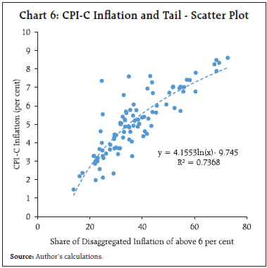
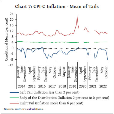
The average inflation over a longer period viz., 2014 to 2022 across the components of CPI-C indicates large variations in some product sub-groups, especially in ‘food and beverages’ viz. ‘meat and fish’, ‘oils and fats’ and ‘spices’ at a higher side with a compound annual growth rate (CAGR) of above 6 per cent. In contrast, the CAGR of ‘sugar and confectionery’ remained lowest, slightly at above 2 per cent (Chart 3).

The variation in CAGRs of the sub-products are reflective of the relative demand for and supply of these products and their intra-year and inter-year variations may represent several generic and specific shocks in the economy. The CAGRs of inflation across States and Union Territories (UTs) have remained in greater sync during the period. The weights (share) of States appeared to have concentrated amongst the top few States, e.g., the top six States, collectively cover more than 50 per cent of weight in the CPI-C basket (Chart 4).

The MoSPI publishes higher levels of disaggregated data of inflation for the larger 22 States/UTs. These cover granularity – by area (rural and urban), by product groups (viz. 6 groups – ‘food and beverages’, ‘pan and tobacco’, ‘clothing and footwear’, ‘housing’, ‘fuel and light’ and ‘miscellaneous’) and by product sub-groups (total 23 sub-groups). The smaller 14 States/UTs, which have individual weights of less than or equal to 0.25 per cent do not have the information at the product sub-group levels. The granular level weights have been taken from CSO (2015). The set of 22 larger States/UTs can be considered to be a proxy for the aggregate CPI-C, as they comprise 98.30 per cent of the aggregate CPI-C of India. It is observed that the compilation of aggregate inflation from the disaggregate (granular) level inflation may have some divergence with the published aggregate inflation prints due to methodological/aggregation issues (Das and George, 2023).

The rest of the analysis in this section and subsequent sections is based on the dataset of 22 large States/UTs. Further, the analysis incorporates appropriate probability-weighted distributions in the computations as exhibited in the Tables and Charts barring one Table (Annex Table A1), which is a simple demonstration of unweighted count of transitions.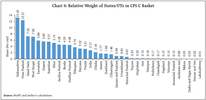

As the prime objective of this study is to track monthly transitions of annual inflation from one level to another at the most granular level⁴, the granular level inflation data of larger States are considered. Based on this disaggregation of data, the gradual decline in the share⁵ of products having high inflation (above 6 per cent) till mid-2017, touching a trough of 13.75 per cent in June 2017, appears to be an important contributor in bringing the CPI-C inflation down and containing it in the desired corridor comfortably. Interestingly, the share of products with inflation between 2 per cent and 6 per cent peaked at around 58 per cent (58.87 per cent in May 2017 and 57.18 per cent in June 2017) during this period reflecting moderate inflation across the board (Chart 5).

Inflation has generally risen with the rise in the share of products having high inflation across the months. However, the relationship does not appear to be linear and rather a log-linear relationship exhibits a better association (Chart 6).

It may be noted that the relative share of products in the high and low inflation bands is expected to offset each other to some extent, in addition to their joint impact with the inflation profile of products in the moderate band of 2 per cent to 6 per cent. The crucial value is indeed not just the share but the conditional distributions in these strata.

The conditional mean, i.e., the average value given that it is in a particular band, has bigger relevance for both the tails, as these are unbounded. As an illustration, the high inflation at 7.35 per cent recorded in December 2019, was driven by a very high conditional mean of higher band (inflation above 6 per cent), i.e., the right tail. This, at 21.98 per cent, happens to be an all-time peak during the months of 2014 to 2022. Surprisingly, while the positive and negative shocks, in terms of share of left tail (24.18 per cent) and right tail (24.55 per cent), were able to offset each other in December 2019, the spread⁶ of their conditional means was quite different from the target of 4 per cent. This was otherwise also quite different from the average profile⁷ of other months (Chart 7).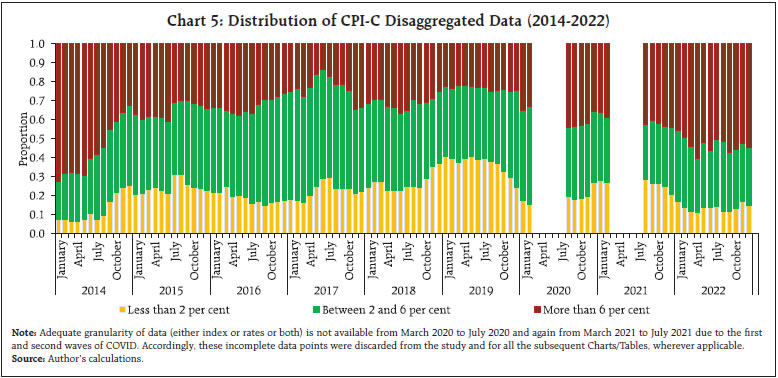

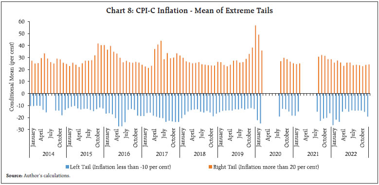Due to the high importance of tails in the inflation disaggregated data, their extreme values were also investigated. These extreme tails demonstrate the vulnerability of inflation prints when the positive and negative shocks fail to offset each other, in terms of their decomposed asymmetric contributions in shaping the final single print of CPI-C inflation (Chart 8).

III. Methodology

A discrete-time first-order Markov process described by a sequence of random variables X(t), t = 0, 1, 2, 3, …, with discrete state space is referred to as a first-order Markov chain or simply as a Markov chain.

We define the stationary probability distribution of a Markov chain with transition probability matrix P if the following conditions hold for all j in S:

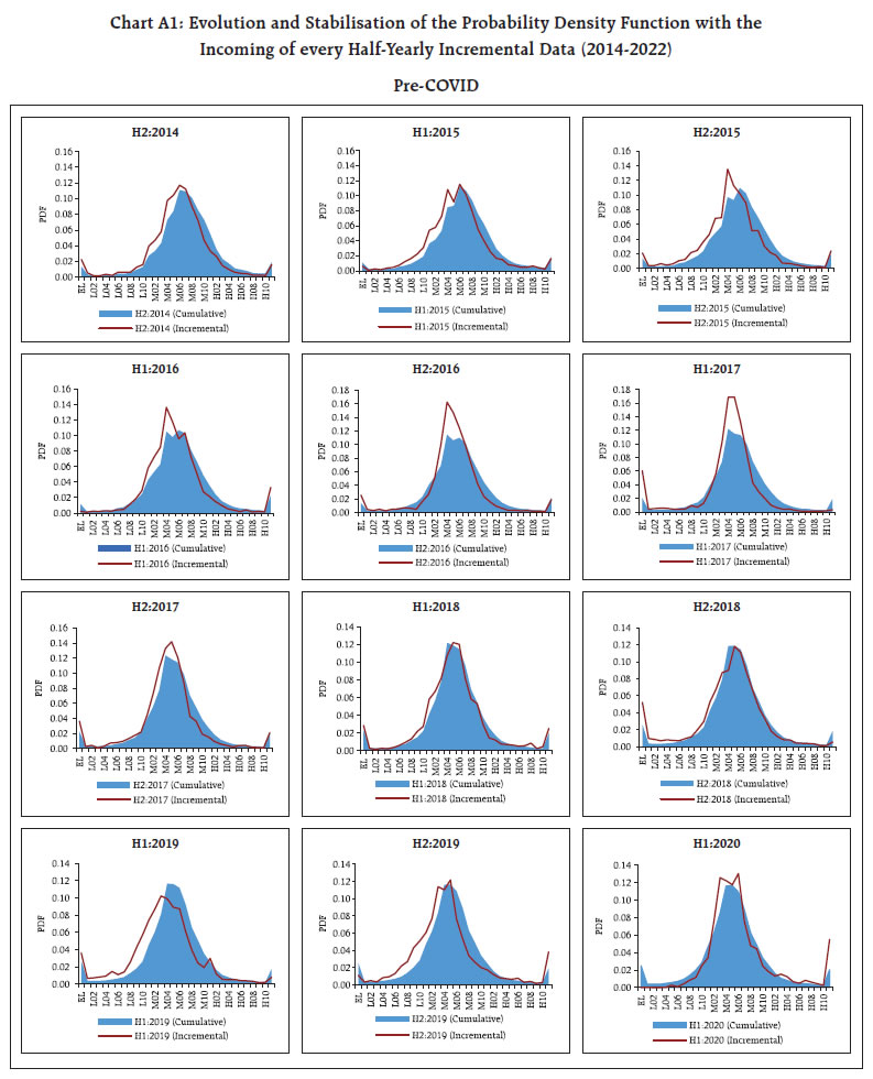
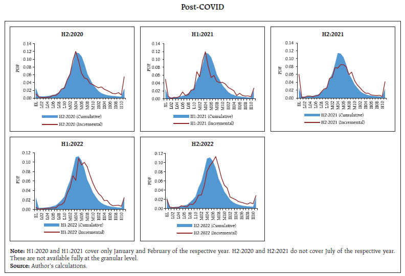
As an extension to the above methodology, we develop a weighted count concept to differentiate a transition of a particular product sub-group across States/UTs and Areas (Rural/Urban) having different weights in the CPI-C basket. This ensures that the transitions through granular data represent aggregate inflation. Accordingly, we now define it as:

The present article attempts to build a simple stochastic process for the transition of CPI-C using the observed (empirical) data as discussed in the introductory section. The transitions of inflation at the granular level are analysed through the stochastic process to derive the long-run steady state of headline inflation. The study uses Markov chains (as defined above) to carry out the exercise. The Markov chains assume discrete state space and discrete time. The discrete-time spaces are considered as “months”, in line with the frequency of CPI-C inflation data. The discrete state spaces are considered as various inflation bands.

The granular dataset of 22 States/UTs is used, as discussed in the second section, to the fullest to investigate every transition. A transition requires pair-wise inflation data for two consecutive months. It may be noted that the data of a particular month is used twice, one for destination (previous month to current month) and the other for origin (current month to next month). However, due to a structural break in the time series leading to the non-availability of complete data from March to July of each year 2020 and 2021, some of the pairs of consecutive months are not available and so are discarded from the study. This way, some of the months are utilised only once (such as February 2020 is used for transition only as a destination), while some others (such as March 2020) are discarded.

We now define our states (viz. the CPI-C inflation bands) in five broad categories, extreme low (EL), low (L), middle (M), high (H) and extreme high (EH) with sub-levels of 10 bands each for the low, middle and high bands. This results in 32 bands for inflation (Table 1).

It may be noted that the tolerance band for inflation for Reserve Bank is 2 per cent to 6 per cent, viz. bands M03, M04, M05 and M06, in the abovedefined classification. However, it may be mentioned that it is meant for the CPI-C All India (Aggregate) inflation and not for its components/granularity. Nevertheless, these bands for the granular data may be useful for policy analysis.

Based on the classification of bands, we track the monthly transitions of the annual inflation at the granular level with appropriate weights assigned to them. Once the transitions from one band to another band for each category of granular-level data are compiled, the transition probability matrix (TPM) of size 32-by-32 is constructed. The same is done for the Pre-COVID, Post-COVID and combined period for the valid pair⁸ of consecutive months. The statistical characteristics of this granular level observed data exhibit clear distinction in the Pre-COVID and Post-COVID periods, in line with the CPI-C Aggregate data (Table 2).

The observed data highlight a shift in the inflation trajectory after the emergence of the COVID pandemic and the subsequent Ukraine war. The evolution of the probability density function of CPI-C inflation at a granular level since 2014 is provided in the Annex, which exhibits how the density is re-shaped after the incoming of every 6-monthly new (incremental) data – both during the pre-COVID and post-COVID periods. The skewness of the density function of the increamental dataset decreased consistently during 2014 and 2015, together with the lowering of inflation. The distribution turned more peaked (leptokurtic) subsequently (during 2016 and H1:2017) with more concentrated values around the central tendency coupled with generally lower extreme values at each end. The frequency of extreme low values increased significantly in H2:2018, which helped aggregate inflation to moderate. The frequency of high extreme values surged in H1:2020, prior to the emergence of COVID. In the post-COVID period, an overall right-ward shift in the inflation distribution is consistently observed with varied intensity coupled with remarkable changes in the densities at extreme ends (Annex Chart A1).

To derive the long-run stationary distribution (LRSD), implementation of a large-sized matrix was possible due to the availability of a large number of observations in the dataset as we chose the highest order of granularity, yielding in a good representation of 1,024 (=32*32) cells in the matrix. As mentioned earlier, we have 990 observations for each of the valid pairs of observations leading to 94,042 observations⁹. The transition matrix for these observations (simple/unweighted count) for the combined period is provided (Annex Table A1) for ready reference for easy demonstration.

It is interesting (and logical) to see that the probability from one extreme band (say, EL) to another extreme band (say, EH) in one month is very unlikely. The vice-versa is also true.

As evident from the Table, there are tiny number of observations of such cases. Accordingly, in a short period of one month, the inflation (y-o-y) is unlikely to either surge or fall drastically.

To better visualise the transitions, we collapse the 32-by-32 matrix into a much smaller matrix (of 3-by-3). It is observed that the persistency of inflation has reduced in the Post-COVID period as compared to the Pre-COVID period in case of low and moderate inflation, while it has increased at a high level. Further, the extreme shifts in transition i.e., from Band A to Band C and also from Band C to Band A have also increased in the Post-COVID phase (Table 3).

Using the above persistency levels of inflation bands in the granular data, the long-run (steady state) mean reversion time of the high inflation band (Band C) appeared to have reduced considerably from the pre-COVID period (3.20 months) to Post-COVID period (2.05 months), which is compensated by an increase in the same for the other two bands. The mean reversion time for Post-COVID indicates that if a transition moves out from band C (either to band A or band B), it is expected to come again to this band (viz. band C) quicker (in around two months), which was 3.20 months for the Pre-COVID era (Table 4).

Based on the transition matrix [P], we can derive a stationary distribution (steady state equilibrium), which is the long-run stationary distribution (LRSD) following these transitions, by solving the set of equations π P = π, where π is a 1*32 row vector and P is a 32*32 matrix. The transpose of the row vector π for these three datasets represents the LRSD (Table 5).

From Table 2 and Table 5, we observe that the long-run steady-state level of inflation would likely be lower than the observed levels, as is seen consistently across the datasets. This signals that the steady state is closer to the mandated target inflation of RBI, as compared to the observed data.

It may be noted that the Pre-COVID dataset is expected to be more robust being longer in series and does not cover one-off episodes of severe events such as COVID and war. Still, we observe a drop of 20-40 basis points in the inflation rate going forward if the current and past transitions hold and other underlying assumptions and conditions continue to prevail.

The nature of the shift (change) in the probability density function from the observed to the LRSD is also worthy of investigation. For example, in the case of the Pre-COVID dataset, although, the shift is small in magnitude, like in the full (combined) dataset (Chart 9), there is an indication of transitions moving towards the central value (Chart 10).

The forecasted probability density of LRSD indicates that the frequency of observations may be slightly more around the central tendency (inflation 0 per cent to 6 per cent) from the observed granular data, which could be compensated with reduced observations in the high inflation bands.

IV. Conclusion

Inflation in India surged since the emergence of the COVID pandemic and the subsequent Ukraine war and became a major policy concern. With the pandemic impact waning, and the supply chains are easing, however, the long-run steady state level for inflation using stochastic transitions at the micro-level data shows a tendency of inflation to tread slowly towards its central value. This study shows that the inflation long-run steady state equilibrium level could be around 4.3 per cent based on the pre-pandemic datasets. The marginal uptick in steady state inflation observed during the pandemic period is likely to be transient and steady state inflation may revert to lower trajectories going forward. The precise speed of the recovery and normalisation of business conditions coupled with evolving situations may dictate how much and how soon the inflation glides onto a lower trajectory.

References

Ascari, G. and Sbordone, A. M. (2014), “The Macroeconomics of Trend Inflation”, Journal of Economic Literature, Vol. 52(3), 679–739.

Behera, H. K. and Patra, M. D. (2020), “Measuring Trend Inflation in India”, Reserve Bank of India Working Paper Series, WPS (DEPR): 15/2020.

Central Statistics Office (2015), “Consumer Price Index: Changes in the Revised Series (Base Year 2012 = 100)”, National Accounts Division, Central Statistics Office, Ministry of Statistics and Programme Implementation.

Das, P. and George, A. T. (2023), “Consumer Price Index: The Aggregation Method Matters”, Monthly Bulletin, Reserve Bank of India, March.

RBI (2017), “Distribution of Inflation in India”, Box II.3, Annual Report 2016-17, Reserve Bank of India, August.

Sinha, R. K. (2018), “Tracking the Stochastic Transition of Inflation in India”, 12th Statistics Day Conference, Reserve Bank of India, 23rd July (Press release – “RBI discusses Measurement and Management of Macro-Economic and Financial Sector Risks at its Twelfth Statistics Day Conference (https://rbidocs.rbi.org.in/rdocs/PressRelease/PDFs/PR2024E74E1ABAEC3426FA7A028611DD7F0EB.PDF).

Annex

^{^} The author is from the Monetary Policy Department (MPD). The author is thankful to Dr. Michael Debabrata Patra for his encouragement and guidance in preparing this article. The views expressed in this article are those of the author and do not represent the views of the Reserve Bank of India.

¹ The emergence of the COVID-19 pandemic and the subsequent Ukraine war led to surges in inflation far from the target point across the globe, including the advanced economies.

² Trend inflation is the permanent or the underlying component of inflation to which actual inflation converges after a shock. Alternatively, this is referred to as steady state inflation (Ascari and Sbordone, 2014). In this article, we use trend inflation and steady state (or steady state equilibrium) inflation interchangeably.

³ Inflation breached the lower threshold two times (1.46 per cent in June 2017 and 1.97 per cent in January 2019), and the upper threshold once (6.07 per cent in July 2016). Noticeably, out of these three breaches, two were minuscule (just 3 and 7 basis points).

⁴ The MoSPI also publishes item-level inflation for all 299 items, as used to construct the CPI-C. However, this is not published by area or by States/ UTs. Accordingly, the overall granularity of the larger States is much higher covering 990 (=2*22*23 - 22) data points. The Sub-group ‘Housing’ is not applicable for Rural areas and, accordingly, is neither available for the States nor for the aggregate CPI-C, and accordingly is not available.

⁵ The share incorporates the appropriate weights of the respective product sub-groups, and not just simple averages, in order to represent CPI-C the way it is compiled.

⁶ The spread (distance) of the conditional mean of the right tail from 4 per cent was at 17.98 per cent in December 2019, while it was only -4.24 per cent for the left tail, which had a conditional mean of -0.24 per cent.

⁷ Based on the simple average of the 98 observed months under the study period, the conditional means of the left tail and right tail are computed as –2.50 per cent and 10.61 per cent, respectively, while it is 4.10 per cent for the body of the distribution.

⁸ The data from January 2014 to December 2022 has 95 valid pairs of consecutive two months, for which granular data is available. This includes 73 pairs for the Pre-COVID period and 22 pairs for the Post-COVID period.

⁹ Eight pairs of observations were missing in the granular dataset, and accordingly, were discarded from the study resulting in 94,042 observations instead of 94,050.