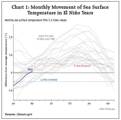
by Saurabh Ghosh^ and Kaustubh^ This study aims to investigate the impact of weather events like El Niño, La Niña, and the Indian Ocean Dipole (IOD) on rainfall and, consequently, on India’s growth and inflation dynamics. It finds that contrary to popular belief, El Niño alone does not necessarily lead to scanty rainfall or high food inflation. IOD often interacts with El Niño or La Niña to determine the actual rainfall pattern and the consequent food inflation. Our empirical findings indicate that the relationship between rainfall and inflation is non-linear and depends on several cofactors. 1. Introduction India’s growth and inflation outlook are significantly influenced by the temporal and spatial patterns and distribution of rainfall during the southwest monsoon season, which generally spans from June to September. With the changing rainfall pattern in recent years, along with the increased intensity and frequency of extreme weather events, there have been several studies analysing the impact of rainfall on growth, inflation, and other macroeconomic indicators in India. For instance, Dilip and Kundu (2020) find that deviations in rainfall can affect food inflation; Ghosh et al. (2021) observe that cyclones can lead to lower output growth, high inflation, and dampened tourist arrivals in the affected regions; and Beyer et al. (2022) suggest that natural disasters like floods can have far-reaching effects on the income and consumption patterns of households, leading to economic disruptions and challenges for individuals and communities. Taken together, these research findings emphasise the significant role of rainfall and extreme weather events in shaping India’s economic landscape. However, studies focusing on understanding the relationship between weather phenomena like rainfall and growth-inflation dynamics have been rather limited. Considering their complex interplay and their overall importance in influencing economic outcomes, we attempt to analyse the influence of El Niño-Southern Oscillation (ENSO) and IOD on Indian agricultural production and inflation. Following an adage that notes “a picture is worth a thousand words”, we consider charts of weather events and relevant macroeconomic variables along with regressions to decipher the impact of weather events on growth-inflation dynamics. The rest of the study is organised as follows: Section 2 deals with extant literature, rainfall forecasts, and actual rainfall. Section 3 reports exploratory data analysis to investigate the relationship between weather events like ENSO and IOD oscillations and rainfall, and the relationship between rainfall and weather events with agricultural growth and inflation. Section 4 deals with regressions to establish the relationship between India’s agriculture, rainfall, and inflation. Section 5 concludes with some policy-relevant observations. 2. Relationship between El Niño and Rainfall In this section, we analyse the rainfall forecast by different agencies and compute their deviations from the actual with an aim to shed light on what could be the plausible reasons for such deviations. 2.1 Forecasts and Actual Rainfall Indian Meteorological Department (IMD) issues various monthly and seasonal forecasts of rainfall for the southwest monsoon season through regular press releases. Private agencies e.g., Skymet started monsoon predictions in the year 2012, and generally it releases monsoon forecasts around a week before IMD. Rainfall forecasts are expressed as a percentage of Long Period Averages (LPA), which acts as a benchmark. The LPA for a decade is the average seasonal rainfall for the past 50 years. Therefore, the LPA is not constant, rather it is changing for each decade. Table 1 indicates that the IMD projections are range-bound. Except for the years 2006 (93 per cent of LPA) and 2016 (106 per cent of LPA), IMD has predicted rainfall in the range of 96-101 per cent of LPA. The table also highlights the errors in monsoon forecast from the actual rainfall, which could be because of the interplay of ESNO oscillations with positive or negative IODs. In the following sections, we would take a deep dive into these interplays of weather events. 2.2 Weather Phenomena: El Niño, La Niña and IOD El Niño and La Niña are weather phenomena caused by the interaction between the surface of the ocean and the atmosphere in the tropical Pacific. El Niño is the phenomenon wherein the water in the eastern Pacific heat up abnormally leading to a reduction and uneven distribution of rainfall in the Indian subcontinent. La Niña is the reverse weather phenomenon wherein sea water in the western Pacific get hot and humid, leading to normal or above-normal rainfall in India. El Niño or La Niña typically starts around end-December, persists for 9 to 12 months, and recurs every 2 to 7 years. It may be mentioned that during 34 per cent of the El Niño years, rainfall was normal or above normal. Chart 1 shows the monthly movement in sea surface temperature (compared to the average temperature) of the eastern Pacific for every El Niño year since 1950, with a purple line tracing the monthly temperature for the year 2023 which has an upward trajectory on April 2023.
 Indian Ocean Dipole (IOD), on the other hand, is defined as the difference between the sea surface temperature (SST) of the western and the eastern Indian Ocean. If the temperature in the west is greater than that of the east, it leads to more rainfall in India (Positive IOD) and vice-versa. IOD can either aggravate or weaken the impact of El Niño on Indian monsoons. Positive IOD may bring good rains to India despite an adverse El Niño condition (Chart 2). It typically recurs after every 3-5 years. Chart 2 (and Annex-Chart A) summarises the interaction of El Niño/La Niña and IOD, and indicates the expected outcomes of these weather phenomena on actual rainfall in India. In a way, this is our Null hypothesis. 2.3 Literature Survey There are a few available studies that have analysed the role of weather events on growth and inflation dynamics. For instance, Challinor et al. (2014) explored the impact of ENSO on global agriculture yields. They found that the impact of El Niño was crop specific. For example, it increased the yield of soybean but had a mixed impact on rice, wheat, and maize yields. However, the impact of La Niña was generally broad-based. Regarding the relationship between rainfall and agriculture GDP, Gulati et al. (2013) noted that 95 per cent of variations in the agriculture GDP growth of India, between 1996 and 2013, can be explained by just 3 factors – public and private investment in agriculture, rainfall, and agriculture price incentives. Bajaj et al. (2019) deep-dived into the relationship between the forecasted rainfall by the IMD and Skymet and found that the forecasts had failed to predict the deficient rainfall of 2002, and 2004 and severe drought conditions of 2009. The authors noted the need to keep a close watch on the weather updates throughout the year for more effective monetary policy formulation rather than relying only on pre-monsoon forecasts. In terms of the relationship between the ENSO and IOD oscillations and rainfall, Ashok et al. (2001) found evidence that ENSOs have a low correlation with Indian southwest monsoon rainfall and IOD have a high correlation. They emphasised that for tracking rainfall patterns, it is important to track IOD oscillations along with ENSO oscillations in India. Thus, the available literature indicates that the relationship between weather events (such as ENSO and IOD oscillation), actual rainfall, and growth-inflation dynamics is quite complex and requires a detailed analysis. We attempt to explore the nature of these intricate relationships through data visualisations and regression analysis. 3. Data 3.1 Data Sources For this study, climate-related data, such as ENSO, IOD and rainfall averages, have been collated from IMD. The data for annual agricultural GVA growth, rabi and kharif food grain production growth, inflation, and food inflation are taken from CEIC. Table 2 lists rainfall, agricultural growth, food inflation, and general inflation during various combinations of ENSO and IOD. | Table 2: Rainfall, Agricultural Growth, and Inflation under ENSO and IOD Events | | | Average Monsoon Rainfall
(% of LPA) | Average CPI Inflation | Average CPI Food Inflation | Average Agricultural GVA Growth | | El Niño - IOD Negative | 88.0 | 5.9 | 6.6 | -0.2 | | El Niño- IOD Neutral | 81.7 | 6.7 | 6.6 | -2.4 | | El Niño- IOD Positive | 94.0 | 5.9 | 5.2 | -1.0 | | La Niña - IOD Negative | 101.7 | 9.4 | 9.7 | 7.3 | | La Niña - IOD Neutral | 99.6 | 6.4 | 6.2 | 3.0 | | La Niña - IOD Positive | 99.0 | 5.5 | 4.3 | 3.5 | | Neutral ENSO - IOD Negative | 102.0 | 9.4 | 9.4 | 9.9 | | Neutral ENSO - IOD Neutral | 98.0 | 5.1 | 4.7 | 5.5 | | Neutral ENSO - IOD Positive | 100.7 | 7.2 | 8.8 | 3.5 | Time Period: 1995-2021
Sources: CEIC, IMD and authors’ calculation. | However, to get a better insight into the relationship between the above-mentioned variables, we have done an extensive exploratory data analysis using creative charts to visualise the complex relationship between them. 3.2 Exploratory Data Analysis (EDA) For this analysis, a year, say 2000, includes the monsoon starting from June 2000, while it represents the agricultural GVA growth for the financial year 2000-01. Similarly, inflation during 2000 indicates the average inflation numbers from April 2000 – March 2001. This convention has been followed uniformly to synchronise agricultural growth and inflation with the appropriate monsoon seasons. 3.2.1 Weather Events and Rainfall As discussed in the previous sections, the relationship between these ENSO and rainfall in India is complex, and other factors such as IOD, the Madden-Julian Oscillation, and local atmospheric circulation patterns may also play a role in determining rainfall patterns over the region. Chart 3 reports the impact of IOD and ENSO on rainfall as percentages of annual rainfall compared to its LPA. It indicates (a) El Niño years have below LPA rainfall if it is combined with Neutral IOD or Negative IOD. (b) Unlike El Niño, the impact of La Niña on total rainfall at the national level is highly volatile, in general, they have hovered around the LPA, and in some years have significantly below LPA (c) In the absence of both El Niño and La Niña, there is also evidence of varied rainfall patterns in India. Irrespective of ENSOs, it is the positive IOD years that have recorded the highest rainfall, on average, as compared with neutral or negative IOD years. Deficient rainfall and severe drought conditions mostly happened only in the El Niño years. But we need to carefully observe the IOD pattern, which could counter the effects of El Niño. 3.2.2 Weather Events and Agricultural Production Next, we explore the relationship between food production and weather events due to ENSO and IOD oscillations. The agriculture and allied sector of GVA mainly comprises crops, fishing, livestock and forestry, of which the first three are crucially dependent on rainfall. Further within the agriculture sector, foodgrains and non-foodgrains production are highly reliant on monsoon performance (Chart 4). Given the heterogeneity within the agriculture and allied sector, it is of policy interest to evaluate how weather vagaries caused by ENSO and IOD oscillations impact the entire sector and the wider economy. Our findings indicate that agricultural GVA growth exhibits lower volatility compared to food grain production growth. This difference can be attributed to sectors such as horticulture, animal husbandry, fisheries, etc., in agricultural GVA, which perhaps provide a buffer against the variability of rainfall. Specifically, kharif food grain production displays higher volatility within the food grain sector than rabi food grain production. This suggests that kharif food grain production is more susceptible to fluctuations in rainfall compared to rabi food grain production (Table 3). 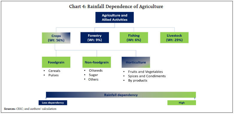 As evident from the left panel (Chart 5), in the Kharif production, El Niño leads to muted or negative kharif growth. La Niña in kharif season with positive and neutral IOD leads to a normal or higher production growth (on average). Even with negative IOD during La Niña, some years (2010, 2014) witnessed decent kharif production growth, mainly because of normal and near-normal monsoon rains. Neutral ENSO in the kharif season generally witnessed positive kharif production growth except for 2012, which could be due to below-normal monsoon rainfall that year. | Table 3: Relative Variance of Annual Growth Rates of Agriculture | | | Variance | Coefficient of Variance | Relative Variance# | | Agricultural GVA | 14.4 | 1.1 | 0.1 | | Kharif Food Grain Production | 96.4 | 5.3 | 0.6 | | Rabi Food Grain Production | 40.0 | 2.3 | 0.3 | | Crops GVA | 23.8 | 1.8 | 0.2 | | Livestock GVA | 18.5 | 0.8 | 0.1 | | Forestry GVA | 8.2 | 0.2 | 0.1 | | Fisheries GVA | 14.4 | 0.7 | 0.1 | | Rainfall | 157.7 | 9.9 | 1.0 | #Relative to rainfall growth
Sources: CEIC; and authors’ calculation. | In terms of rabi season food production growth (Chart 6), in line with the expectations, the El Niño years have lower (mostly negative) rabi production growth. La Niña years, on the other hand, reported good rabi production growth, except for 1995 (possibly due to base effect as the previous two years had good production growth) and 2000 (due to below normal monsoon in 2000 despite a La Niña year). In years of neutral ENSO, the volatility of rabi production is generally high, although, on average, it remains higher compared to La Niña and El Niño years (Chart 6). For instance, during neutral ENSO, rabi production growth varies from 12 per cent in 1996 (attributable to a base effect, as 1995 had negative rabi production growth) to a negative 1 per cent in 2018 (due to below-normal monsoon rains experienced that year). 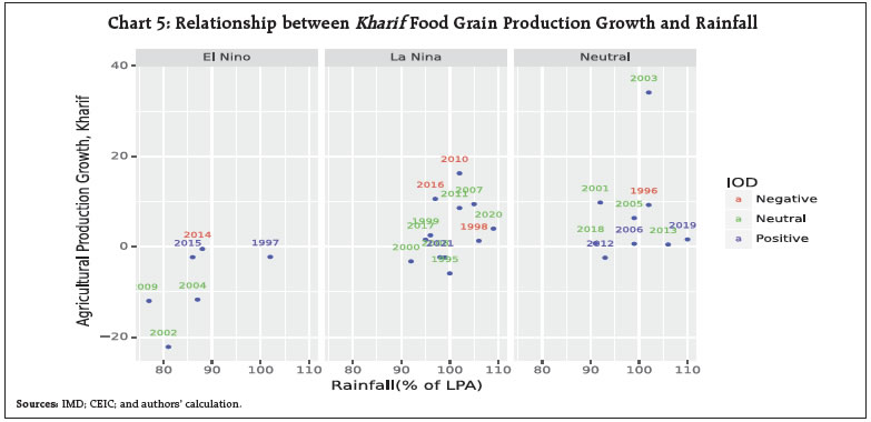 In terms of the growth of agricultural GVA, ENSO seem to have a profound impact, as during El Niño years agricultural GVA was observed to hover around zero growth, even with some years witnessing significant negative agricultural production growth rates. La Niña and neutral years are having wide variations, from high positive to negative growth rates. However, it is La Niña combined with neutral IOD that has, on average, recorded good agricultural GVA growth. Further, El Niño with negative IOD is giving negative or close to zero growth in the agricultural GVA (Chart 7). If, however, negative IOD is combined with La Niña or Neutral ENSO, then its effects have been largely neutralised. This could explain the large increase in agricultural GVA in 1996, 1998, 2010, and 2016 (Chart 7). 
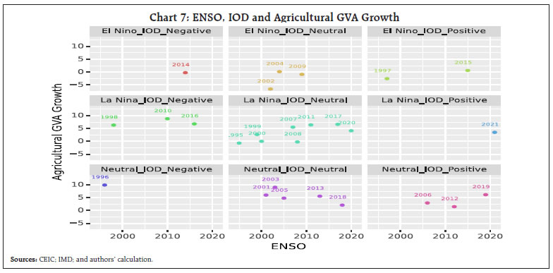 Thus, we can infer that in general El Niño years recorded lower or negative agricultural GVA growth. La Niña years are generally marked with positive agricultural GVA growth, except for 1995 (that was an exceptional year due to a drop in rice production in Punjab and Haryana because off excessive off-season rainfall1). However, in terms of ENSOs neutral periods are clear winners in terms of agricultural GVA growth, and this is irrespective of IOD status (Chart 7). It may be noted that weather events like ENSO and IOD affect agriculture not only through rainfall but through other channels also such as temperature, global commodity price fluctuation, and frequency of extreme weather events (like floods, drought, etc.). Thus, weather events’ interaction with agriculture and economics needs to control for several other factors in a multivariate framework. 3.2.3 Weather Events and Manufacturing Output The impact of weather events on the industrial sector in India can be assessed in terms of sectoral interlinkages between agriculture and industry. In the Indian context, weather conditions could adversely affect agriculture growth, which in turn impacts industrial production by affecting the supply of wage goods, agrarian inputs, and demand for industrial goods. The slow growth of agricultural income could impact consumer demand, which in turn affects the industrial output (Ahluwalia, 1991). As the agricultural sector contributes significantly to rural income, the private consumption demand is considerably affected by the levels of farm incomes. This is more applicable in the case of consumer goods, which carry a significant weight (of about 28 per cent) in the index of industrial production. Thus, adverse growth in the GVA originating from the agricultural sector as a result of adverse weather conditions could restrain demand for industrial goods and the expansion of output. The supply side effects of adverse weather conditions on the industrial output is transmitted through a reduced supply of raw materials used in the industries. The impact is twofold: one, the supply is reduced; second, the prices of such inputs for the industry tend to rise, thus raising the overall cost of production. The agro-based industries which constitute around 7-10 per cent of the value added of the industrial sector, could be more severely affected by an adverse shock on agriculture since such industries entirely depend on the latter for requirements of their raw material. Data broadly support the above transmission channels as manufacturing GVA growth was in general on the lower side in the El Niño years and negative IOD years (Chart 8). The exceptions were 1997 and 2019, when despite positive IOD manufacturing GVA growth fell significantly, which could be due to other factors, e.g., Asian Financial Crisis in 1997 and NBFC problems in 2019. 3.2.4 Services Sector Activity and Its Linkages The conjectural projection for the impact on real activity in the services sector is difficult to make because of the weaker, not-so-quantifiable nature of impact and the lack of information on informal sector activities. It is, nevertheless, necessary to make some informed judgement about the real activity in the services sector, given that the share of the services sector in aggregate output has increased from less than one-third in 1950-51 to around 60 per cent in recent years. Unlike industry, services are perhaps not entirely affected by agriculture. Data on rainfall and the services sector bring up the limited role of weather events in this sector (Chart 9). 3.2.2 Weather Events and Food Inflation Like any other commodities, food prices are functions of supply and demand. A scanty monsoon is often considered as one of the most important supply shocks, leading to price pressures. Persistent food inflation is often worrisome for a monetary policy authority because of its second-round impacts. Food inflation also plays an important role in the inflation expectation of households2, which is a key factor in the New Keynesian Phillips (supply) curve. For an emerging market economy like India, food inflation impacts headline inflation quickly mainly because of the high share of food items in households’ expenditure, thereby leading to a large share of food items in CPI inflation, and wage indexation to CPI inflation (Anand 2014)3. 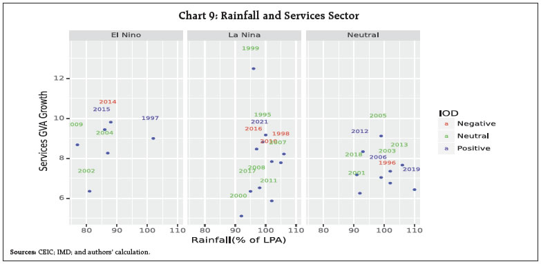 However, there hasn’t been a one-to-one correspondence between monsoon and food inflation in India. Food inflation was high in 2009, which was mainly due to deficient rainfall. Notwithstanding better rainfall, high food inflation persisted in 2010 and partly in 2011, spilling over to headline inflation. Similarly, there is a dichotomy between ENSO weather events and their impact on food inflation. Recently, while some commentaries have raised concerns about El Niño posing a potential risk to inflation dynamics in FY 24, many others have argued that even in the presence of El Niño, its impact on Indian economic growth and inflation would be limited (Nadhanael et al.,2023). In view of its policy importance and relevance, the following sections critically evaluate the impact of ENSO and IODs on food inflation. Contrary to expectations, median food inflation (bold horizontal lines in the boxplot) was low during the El Niño periods. Moreover, during El Niño, La Niña, and Neutral years the medians were close, indicating similar food inflation outcomes. However, some El Niño years were marked by extreme observations in terms of inflation, indicated by far-away dots (e.g., 2009), which was a drought year (Chart 8). Food inflation volatility was indeed higher during the La Niña period, as indicated by the height of the boxplot and the long whiskers. Notwithstanding a few extreme observations (e.g. 2012, 2013), in terms of median inflation and variability, neutral ENSO years ranged between El Niño years and La Niña years (Chart 10). The negative IOD years, on the other hand, clearly witnessed higher average food inflation than neutral or positive IOD. Notwithstanding low median food inflation, the neutral IOD periods were marked by extremely volatile food inflation, as evident from the length of the boxplot (Chart 11). They also indicated the presence of some extreme observations, e.g., 2009, 2008, and 2013, due to extreme weather events (severe drought of 2009 and above-normal rainfall in 2013). Food inflation during the positive IOD period was higher than the median of Neutral IOD periods. Despite positive IOD, inflation was high in the year 2012. Thus, data indicate that El Niño may not always result in very high food inflation. But due attention is needed on IOD, as negative IOD often coincides with very high food inflation (Chart 9). 3.2.5 Weather Events and Headline Inflation As food inflation constitutes a large component of the CPI basket, an association of headline inflation and weather events like ENSO and IOD oscillation often mirrors that of food inflation. The El Niño years have on average lower inflation and less variability compared to the La Niña years, except for the severe drought year of 2009 (Chart 12). The La Niña years have very high variability in terms of inflation. The median inflation in neutral ENSO years is low but there are some cases of high inflation periods (2012) during the neutral ENSO years.
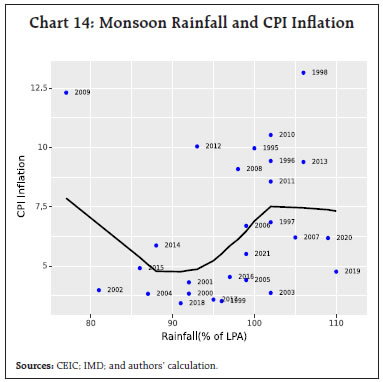
On the other hand, the negative IOD years have on average higher inflation than neutral or positive IOD. While the median inflation for Neutral IOD is rather low, mainly because of the bunching of a few low inflation years (e.g. 2000, 2017 and 1999), the Neutral IOD boxplot is marked with extreme observations Positive IOD years have moderate inflation with low variability. 3.2.6. Monsoon and Growth-Inflation Dynamics The scatter plot of Indian agricultural GVA points to its dependence on monsoon rainfall, which is indicated by the positive slope of the regression line over the years with agricultural GVA growth on the Y-axis and monsoon rainfall (per cent of LPA) on the X-axis (Chart 13). Besides the supply of agricultural output, rural income, and consumption are the major determinants of aggregate demand. In this vein, the smooth plot (i.e., without imposing any restrictions on curve fitting) of food inflation and monsoon rainfall indicates a rather non-linear relation, which could be because of several shift parameters influencing demand and supply curves (Chart 14). 
 Finally, we report the correlation heatmap of the relevant variables included in the above analysis (Chart 15). It indicates a significant correlation between annual rainfall throughout the year and seasonal (monsoon) rainfall. This could be because, in India, approximately 75 per cent of the annual rainfall occurs during the monsoon season. Additionally, we observe a strong correlation between headline CPI inflation and CPI food inflation. As indicated earlier, this could be attributed to the high weight of the food component in the consumer price index (CPI). The correlation matrix also indicates a strong association of agricultural growth variables with rainfall. However, the contemporaneous correlation between food and headline inflation and rainfall was found to be statistically weak, which could be due to the effects of other control variables and functional specifications. In the next section, we attempt a formal evaluation of the same in a multivariate regression framework where we introduce appropriate non-linearities.  4. Empirical Findings 4.1 Rainfall and agricultural growth The impact of rainfall on agricultural growth was examined through a simple autoregressive model augmented by monsoon rainfall (per cent of LPA). Models 1, 2, and 3 consider different dependent variables, i.e., annual agricultural GVA growth, annual rabi food grain production growth, and annual kharif food grain production growth, respectively. Each model includes lagged values of the dependent variable, to account for the base effect, persistence, and monsoon rainfall (per cent of LPA) as independent variables. In all the models, the coefficients of monsoon rainfall are positive and statistically significant, indicating that higher monsoon rainfall, on average, leads to higher agricultural growth. Further analyses of the coefficients of annual rainfall growth indicate that both kharif food grain production growth and rabi food grain production growth are dependent on rainfall. The negative coefficients of the lagged dependent variables in these models could indicate the base effects. | Table 4: Regression results explaining Agricultural Growth | | Dependent Variable | | | Agricultural GVA Growth | Rabi Food Grain Production Growth | Kharif Food Grain Production Growth | | Model 1 | Model 2 | Model 3 | | Constant | -19.3*** | -37.3*** | -38.72** | | Lag Dependent Variable | -0.48*** | -0.43*** | -0.55*** | | Rainfall Growth (Annual) | 0.24*** | 0.43*** | 0.42** | | R- square | 0.57 | 0.57 | 0.52 | | Adjusted R -square | 0.54 | 0.54 | 0.48 | Time Period of the Model 1, Model 2 and Model 3 – 1993-2020
Note - * denotes level4 coefficient statistically significant at 15 percent significance, ** denotes significant at 5 percent significance level, and *** denotes significant at 1 percent significance level. | 4.2 Rainfall and Inflation As food constitutes a major portion of the CPI consumption basket, it is the most likely channel through which rainfall and consequent agricultural growth would impact the overall CPI inflation. Therefore, to analyse the effect of rainfall and agriculture growth on inflation, we regressed each of the annual CPI food inflation and CPI headline inflation, on the amount of contemporaneous monsoon rainfall. Additionally, it is important to note that we included both monsoon rainfall and the square of monsoon rainfall as explanatory variables in all models to account for the non-linear relationship between rainfall and inflation, (as observed in Chart 14). Further, we controlled for agriculture growth rates and international commodity price inflation (Bloomberg data), as India is a major non-food commodity importer. The results of the regressions are summarised in Table 6. Among the estimates, model 1 uses annual CPI food inflation and headline CPI inflation each as a dependent variable, it includes the lagged dependent variable, growth in kharif food grain production, lag of rabi food grain production5, current year monsoon rainfall as the percentage of the long-term average (LPA) and its square as explanatory variables. In model 2, we have regressed each of the annual CPI food inflation and headline CPI inflation with their lags (AR1), annual agriculture GVA growth, lag of agriculture GVA growth, monsoon rainfall, as a percentage of the long-term average (LPA), and its square term. Model 3, controls for international commodity price inflation, in addition to the set of independent variables used in Model 2. Among the control variables, both rabi and kharif food grain production growth coefficients are statistically significant and negative, suggesting that an increase in agricultural supply leads to lower food inflation. The magnitudes of both coefficients are similar, indicating that the productions of both seasons play an almost equal role in food inflation. Similarly, in Model 2, the coefficients of current year agricultural GVA growth and its lag are negative, indicating that higher agriculture supply leads to lower food inflation. The magnitude of both coefficients is nearly equal, indicating that both the current-year agricultural GVA growth and previous-year agriculture growth have almost equal role in reducing food inflation. However, the lagged annual food and headline inflation coefficients are positive and statistically significant in all three models, indicating persistence in inflation, possibly due to adaptive inflation expectations (Dua and Goel, 2021). Finally, coefficients of international commodity prices inflation are positive in sign, indicating that after accounting for rainfall and agriculture growth they have a positive impact on both food and headline inflation. In these models, the coefficients of rainfall reveal the non-linear relationship between rainfall and inflation. The coefficient for rainfall is negative, while the coefficient for the square of rainfall is positive. This indicates a parabolic relationship where an increase in rainfall up to a certain threshold leads to lower headline and food inflation, but beyond that threshold, further increases in rainfall may result in higher inflation. This relationship can be attributed to the positive impact of rainfall on aggregate supply up to a moderate level, while excess rainfall beyond the threshold often leads to crop damages coupled with supply chain disruptions. In Model 3, the negative rainfall coefficients were statistically significant, indicating the importance of rainfall on inflation. Although the coefficients of rainfall and its square are not statistically significant in other models, their p-values are relatively low. This lack of statistical significance could be attributed to the endogeneity problem associated with food production and inflation, rather than the insignificance of the relationship between rainfall and its square with inflation. We would address the endogeneity issue in a 2SLS setup using rainfall as an instrumental variable. 4.3 Rainfall, Agricultural Output, and Inflation: Instrumental Variable To address the issue of possible endogeneity between agriculture growth and inflation in the previous regression models, we have employed the Two-stage Least Squares (2SLS) method to refine the results in section 4.2. This method allows us to mitigate the endogeneity problem by introducing instrumental variables, specifically the growth in rainfall. Rainfall serves as an exogenous variable, as economic factors such as agricultural growth and inflation do not have a direct impact on it. However, rainfall does impact both inflation and agriculture growth. Therefore, it is a suitable instrument to address the endogeneity issue and determine the impact of agriculture growth on inflation. We utilise the predicted values of agricultural GVA growth, rabi food grain production growth, and kharif food grain production growth derived from the regressions (stage 1), where these variables were regressed on annual rainfall growth and their own lag respectively. In Model 1, we use the predicted values of kharif food grain production growth and rabi food grain production growth as control variables. Similarly, in Models 2 and 3, we use the predicted value of agricultural GVA growth as a control variable6. The results of regressions are summarised in Table 5. In the 2SLS regressions, the coefficients of monsoon rainfall and its square are statistically significant and exhibit patterns consistent with the regressions in Section 4.2, thereby confirming the presence of a non-linear relationship between monsoon rainfall and inflation, even after controlling for agriculture growth. This suggests that monsoon rainfall influences food and headline inflation through channels beyond its impact on agriculture growth. The coefficients of kharif food grain production growth and lag of rabi food grain production growth continue to exhibit negative values, and their magnitudes remain nearly equal for both food and headline inflation, though their statistical significances remain weak. This finding suggests that the production levels of both seasons are significant determinants of food and headline inflation, even after accounting for endogeneity between agriculture growth and inflation. The low level of significance of agricultural growth variables may be attributed to the filtering of variations in these variables during the first stage of the 2SLS regression, to address the endogeneity issue. Moreover, the impact of international commodity prices on food inflation was positive, indicating the influence of international commodity prices on domestic inflation. | Table 5: 2-SLS Regression (with Rainfall as instrumental variable) results explaining variations in headline and food Inflation | | Dependent Variable | Model 1 | Model 2 | Model 3 | | CPI Food Inflation | Headline CPI Inflation | CPI Food Inflation | Headline CPI Inflation | CPI Food Inflation | Headline CPI Inflation | | Explanatory Variables | | | | | | | | Constant | 193.55** | 121.47** | 186.76** | 117.89** | 205.5* | 132.3* | | Lag of Dependent Variable | 00.39** | 0.52*** | 0.40** | 0.52** | 0.50** | 0.60*** | | Monsoon Rainfall (% LPA) | -4.23** | -2.63** | -4.02** | -2.51** | -4.42** | -2.81** | | Square of Monsoon Rainfall (% LPA) | 0.0235** | 0.0145** | 0.0223** | 0.0139** | 0.024** | 0.015** | | Control Variables | | | | | | | | Predicted Kharif Season Food Grain Production Growth | -0.33 | -0.22 | | | | | | Lag of Predicted Rabi Season Food Grain Production Growth | -0.55 | -0.32 | | | | | | Predicted Agricultural GVA Growth | | | -0.67 | -0.46 | -0.50 | -0.36 | | Lag of Predicted Agricultural GVA Growth | | | -0.67 | 0.40 | -0.60 | -0.34 | | Lag of International Commodity Prices Growth | | | | | 0.09 | 0.06 | | Adjusted R-square | 0.35 | 0.40 | 0.35 | 0.40 | 0.37 | 0.42 | | Note: * denotes coefficient statistically significant at a 15 per cent significance level (footnote 4), similarly, ** denotes significant at 5 percent significance level, and *** denotes significance at a 1 per cent significance level. Time Period of the Model 1, Model 2 and Model 3 – 1994-2020 |
| Table 6: Regression results explaining variations in headline and food Inflation | | Dependent Variable | Model 1 | Model 2 | Model 3 | | CPI Food Inflation | Headline CPI Inflation | CPI Food Inflation | Headline CPI Inflation | CPI Food Inflation | Headline CPI Inflation | | Explanatory Variables | | Constant | 91.44 | 60.74 | 91.71 | 65.84 | 117.5* | 84.26* | | Lag of Dependent Variable | 0.62*** | 0.70*** | 0.51*** | 0.62*** | 0.61*** | 0.71*** | | Monsoon Rainfall( % LPA) | -2.08 | -1.35 | -2.05 | -1.43 | -2.50* | -1.82* | | Square of Monsoon Rainfall ( % LPA) | 0.012 | 0.008* | 0.012* | 0.008* | 0.015* | 0.01* | | Control Variables | | | | | | | | Kharif Season Food Grain Production Growth | -0.21** | -0.13** | | | | | | Lag of Rabi Season Food Grain Production Growth | -0.30** | -0.18** | | | | | | Agricultural GVA Growth | | | -0.51* | -0.28* | -0.48* | -0.25* | | Lag of Agricultural GVA Growth | | | -0.51** | 0.29* | -0.53** | -0.27* | | Lag of International Commodity Prices Growth | | | | | 0.10* | 0.06* | | Adjusted R -square | 0.43 | 0.48 | 0.42 | 0.45 | 0.45 | 0.48 | Note: * denotes coefficient statistically significant at 15 percent significance level, similarly, ** denotes significant at 5 percent significance level, and *** denotes significant at 1 percent significance level.
Time Period of the Model 1, Model 2 and Model 3 – 1990-2021 | 5. Conclusion Monetary policy hinges on inflation expectations, which in turn depend on food inflation. In India, the agricultural sector is considerably dependent on monsoon rainfall. It is generally believed that weather events (e.g., El Niño, La Niña, and the Indian Ocean Dipole) have significant impacts on rainfall and thereby influence growth-inflation dynamics. Considering their importance, we explore the impact of these weather events on India’s growth and inflation. Our finding suggests that contrary to popular belief, El Niño, by itself, may not lead to a deterioration in macroeconomic stability. There were years when, despite El Niño, rainfall was close to normal and inflation remained benign. The analysis indicates that it is indeed the IOD that often interacts with El Niño or La Niña to determine the actual rainfall. This is evident as average inflation was higher during the negative IOD years as compared with the neutral or positive IOD years. La Niña years also experienced a wide range of agricultural growth and inflation, depending on the corresponding IOD oscillation status and other exogenous factors. Further, our analysis indicates that while higher rainfall leads to higher agriculture growth (in both the rabi and kharif seasons), the relationship of inflation with rainfall is non-linear. This could be because rainfall impacts the food inflation dynamics through agricultural growth. At the same time, other exogenous factors, such as international commodity prices also influence these growth-inflation dynamics. In conclusion, our data analysis highlights that a single adverse weather event (e.g., El Niño) may not be a threat to macroeconomic stability, but we need to be vigilant on other factors, such as IOD oscillations, local supply chain disruptions caused by acute climate events, and global commodity prices. References Ahluwalia, D. (1991), “Drought Proofing in the Indian Foodgrain Economy”, Indian Journal of Agricultural Economics, 46(902-2018-2823), 111-120. Anand, R., Ding, D., and Tulin, M. V. (2014), “Food Inflation in India: The Role for Monetary Policy”, International Monetary Fund. Ashok, K., Guan, Z., and Yamagata, T. (2001), “Impact of Indian Ocean dipole on the relationship between the Indian Monsoon Rainfall and ENSO”. Geophysical Research Letters - GEOPHYS RES LETT. 28. 10.1029/2001GL013294. Bajaj, P., Suganthi, D., Kumar, R. and Mukherjee, A. (2019), “Will the Weather Gods Smile or Frown? Evaluating Monsoon Forecasts”, RBI Bulletin, June_ Dilip A., and Kundu, S. (2020), “Climate Change: Macroeconomic Impact and Policy Options for Mitigating Risks”, RBI Bulletin, April. Dua P. and Goel D. (2021), “Inflation Persistence in India”, Journal of Quantitative Economics 19, 525–553 Iizumi, T., Luo, JJ., Challinor, A., et al. (2014), “Impacts of El Niño Southern Oscillation on the Global Yields of Major Crops”, Nat Commun 5, 3712 https://doi.org/10.1038/ncomms4712 Gulati, A., Saini, S. and Jain, S., (2013), “Monsoon 2013: Estimating the Impact on Agriculture”, Working Papers, eSocialSciences. Ghosh, S., Kundu, S., and Dilip, A. (2021), “Green Swans and their Economic Impact on Indian Coastal States”, Reserve Bank of India Occasional Papers, 42(1). Malik, A., Li, M., Lenzen, M., Fry, J., Liyanapathirana, N., Beyer, K., Boylan, S., Lee, A., Raubenheimer, D., Geschke, A., and Prokopenko, M. (2022), “Impacts of Climate Change and Extreme Weather on Food Supply Chains Cascade across Sectors and Regions in Australia”, Nature food, 3(8), 631–643. https://doi.org/10.1038/s43016-022-00570-3 Nadhanael, G. V., et al. (2023), “State of the Economy”. RBI Bulletin, April
Appendix
|