by Deepmala, Sunil Kumar and Bipul Ghosh^ This study investigates the drivers of private consumption in India, both in the short and long term. The findings reveal a long-run relationship between real private consumption, income and wealth, indicating a strong correlation between consumption and income over time. Additionally, factors such as interest rates, consumer and government indebtedness, inflation, and uncertainty impact short-term private consumption. Furthermore, the study highlights the asymmetric impact of interest rates, with monetary policy being more effective in containing private consumption rather than stimulating it. Monitoring these factors becomes crucial for accurately assessing the evolving domestic demand conditions. Private consumption is a key driver of aggregate demand in India, like many other economies. Although its share has come down over the years, it still constitutes the largest part of aggregate demand –around 56 per cent during 2012-13 to 2019-20 and contributed about 59 per cent to real GDP growth on an average during this period. The pandemic-induced large loss of lives, livelihoods, and consumer confidence, however, dented private consumption substantially – it contracted by 5.2 per cent during 2020-21 and pulled down real GDP by 5.8 per cent in the same year. Amidst fiscal and monetary stimuli, private consumption rebounded and grew by 11.2 per cent and 7.5 per cent during 2021-22 and 2022-23, respectively; real GDP expanded by 9.1 per cent and 7.2 per cent, respectively, during these years, exhibiting strong co-movements. Considering the paramount contribution of private consumption to aggregate demand and growth, an analysis of its macroeconomic drivers assumes importance for a more informed, forward-looking assessment and navigation of the business cycles efficiently. Income, wealth, inflation, interest rate, and future expectations/ uncertainty, among others, are major potential determinants of short- and long-run private consumption (Singh, 2012; Vihriälä, 2017; Wong, 2017; Dossche, et al., 2018). In the long-run, income and wealth drive private consumption according to the insights provided by the seminal works such as “permanent income hypothesis (PIH)” and “life cycle hypothesis (LCH)” (Freidman, 1957; Modigliani, 1954; Ando and Modigliani, 1963; Fernandez-Corugedo, 2004). PIH postulates that consumers decide their expenditure based on their long-term view of the likely resources available to them. According to LCH, forward-looking consumers maximise their lifetime utility subject to the lifetime resources available to them – households save more at a young age to finance consumption post-retirement. Any variation in asset prices and wealth changes the expected income and may trigger a readjustment in the current consumption. On the other hand, factors such as interest rates, inflation, availability of credit, government indebtedness (Ricardian equivalence phenomenon), and uncertainty influence private consumption in the short term. With inflation reaching multi-decadal highs across countries during 2022-23, its role in dragging down private consumption has attracted attention. For example, in the Indian context, as noted by Patra (2023), inflation ruling above 6 per cent is inimically harmful for growth and is showing up in the deceleration of private consumption spending and the moderation in sales growth in the corporate sector. Against this backdrop, we empirically examine the long-run and short-run macroeconomic drivers of private consumption in India in an error correction framework for the period 2004-2019, using quarterly data. We have chosen pre-pandemic period for the empirical analysis to have robust inferences as the pandemic led to a massive structural break in data. The empirical analysis indicates a long-run co-integrating relationship between real private consumption and income and wealth, with income elasticity close to unity pointing towards a strong co-movement of consumption and income over time. Amongst the short-run drivers, besides income and wealth, real interest rate; inflation; and indebtedness of households and government are found to be impacting private consumption. The paper also explores the potential asymmetric effect of monetary policy easing and tightening cycles on private consumption. The analysis suggests an asymmetric impact: monetary tightening dampens private consumption more than the expansionary effect of an equivalent easing of interest rate. The anatomy of the remaining study is as follows: a brief review of literature is discussed in Section 2; data and methodology are furnished in Section 3; Section 4 describes the empirical findings including the asymmetric impact of the monetary policy on private consumption; and concluding observations are given in Section 5. 2. Literature Review Consumption and its drivers have received wide coverage in economic research. The seminal work of Keynes on General Theory (Keynes, 1936) identifies the relationship between income and consumption as a key macroeconomic relationship wherein real consumption is mainly determined by real disposable income, with a supplemental role for wealth, credit, taxes, expectations, and aggregate price levels. Extending the relationship between consumption and income beyond Keynes’s “absolute income hypothesis”, Duesenberry (1949) postulates that consumption is also influenced by previously achieved consumption levels, implying that once a particular level of consumption is attained, it becomes difficult to cut it significantly. Modigliani (1954) focuses on the “lifecycle hypothesis” wherein households consume a constant portion of the present value of their lifetime income – accordingly, they save at a young age to finance consumption post-retirement. Freidman’s (1957) “permanent income hypothesis (PIH)” distinguishes between current income and permanent income (income expected during lifetime) and argues that consumers decide their expenditure based on the latter reflecting their long-term view of the likely resources available to them. While permanent income is regarded as average income over the long run which is influenced by several factors such as accumulated or inherited wealth/capital, occupation, environment etc., the transitory component of income is largely saved, with minimal impact on current consumption. Hall (1978) by combining rational expectations theory with permanent income hypothesis suggests that consumption follows a random walk process. Empirical studies also suggest the response of consumption to be asymmetric to the positive and negative income shocks. Jawadi and Léoni (2012) find the relationship between income and consumption as non-linear and cyclical. According to Bunn et al. (2018), the marginal propensity of consumption (MPC) of negative income shocks is higher than that of positive income shocks in the UK. Similar results are found in case of the Netherlands (Christelis et al., 2019). The impact of wealth, especially housing and financial assets, on consumption has been studied extensively which is also relevant for monetary policy transmission. Wealth could affect private consumption through various channels, viz., i) realized wealth, ii) unrealized wealth, iii) budget constraints, iv) liquidity constraints and v) substitution effects (Cooper and Dynan, 2016; Paiella and Pistaferri, 2017; Jawadi et al., 2015). Some studies find housing wealth affecting consumption more than financial wealth (e.g., Benjamin et al., 2004; Bostic et al., 2009; Case et al., 2013). The impact of housing and financial wealth on consumption may be cyclical and asymmetric across countries (Lettau and Ludvigson, 2004). The asymmetric impact can be due to income uncertainty and risk aversion (Carroll and Kimball, 1996), varying perceptions of liquidity (Shefrin and Thaler, 1988), and the combination of liquidity constrains and business cycles (Apergis and Miller, 2006). According to Schooley and Worden (2008), households’ spending gets a boost from an increase in their assets from home equity. In the Indian context, Singh (2012) finds that a 10 per cent rise in real stock wealth increases the consumption demand by 0.3 per cent, consistent with estimates for some emerging market economies. Khan et al. (2015) estimate consumption function for South Asian countries including India and they conclude that while consumption depends on current income in the short run, consumers foresee their future income and accordingly make consumption decisions based on permanent income in the long run. Amongst other determinants of private consumption, interest rate impacts consumption through income and substitution effects – these effects could operate in opposite directions, rendering the aggregate impact on consumption uncertain and mixed, depending upon household-specific characteristics. Some studies have found an inverse relation (e.g., Boskin, 1978; Mishkin, 1976; Gylfason, 1981; Kozlov, 2023), while others document a positive relation (e.g., Springer 1975). Kozlov (2023) finds that a decrease in the interest rate boosts consumption substantially in the short-run, which diminishes over time. Gourinchas and Rey (2018) underline that co-movements in real interest rates and real consumption do not follow a systematic trend. Some studies have found the impact of interest rates on consumption to be weak (Kapoor and Ravi, 2009; MacDonald et al., 2011; Hviid and Kuchler, 2017). Interest rate fluctuations also affect households’ consumption through “balance sheet channel” by influencing property prices (the wealth effect) and cash flows through mortgage payments. Mian and Sufi (2014) underline that a large fraction of the consumption decline during the Great Recession period could be potentially attributed to “household balance sheet” channel. Several studies have found that an easing of borrowings constraint bolsters household consumption during normal/ boom phase, but excessive borrowings (leverage) adversely impact their consumption when the economy is undergoing through a stress phase (e.g., Mian and Sufi, 2011; Dynan, 2012; Baker, 2018). High household debt built up in the US during the boom phase led to weaker economic conditions during the burst phase as several shocks hit households: a decline in housing prices, an increase in borrowing constraints, and a fall in housing and equity wealth raising debt-asset ratio beyond acceptable levels (Mian and Sufi, 2011). Highly indebted households cut consumption substantially in response to negative income shocks (Baker, 2018). De Nardi et al. (2017) argue that precautionary savings in response to an increase in labour market risk lead households to substitute consumption expenditures with safe assets such as government securities. The validity of the Ricardian equivalence hypothesis (REH) is examined by Ayunasta et al. (2020). Their findings show that Indonesian household consumption is not significantly impacted by the government’s external debt, but other factors such as gross domestic product, tax revenue, government spending, and government budget surplus / deficit exert statistically significant influence on it. Dooyeon Cho and Dong-Eun Rhee (2013) find nonlinear effects of government debt on private consumption - a higher level of government debt crowds out private consumption to a greater extent. A thorough empirical analysis on the relationship between inflation, interest rate and GDP and household consumption are provided by Osuji Obinna (2020). The author finds that a high inflation rate can cause distortion and uncertainty in the economy so that it will reduce aggregate consumption and dampens economic growth. 3. Model Specifications Drawing upon the underlying economic theories and literature review in the previous section, the potential long - and short-run determinants of consumption demand are: (1) income and wealth, (2) interest rate; (3) credit availability and consumer indebtedness; (4) fiscal policy and government indebtedness; (5) Inflation; (6) uncertainty; (7) demographic change. For our study, personal disposable income (PDI)1 is taken for income category while stock market capitalisation and Bombay Stock Exchange (BSE) index are considered for wealth effect. The interest rate is proxied by alternative measures such the weighted average call rate (WACR); weighted average lending rate (WALR) on outstanding loans of commercial banks; 1-year g-sec yield (1YRGSY); and 10-year g-sec yield (10YRGSY). Households’ indebtedness is captured through personal loans outstanding, while central government debt is a measure of government indebtedness to capture the Ricardian equivalence effects. Inflation is measured by private consumption deflator. The uncertainty indices and crude oil prices are taken to capture uncertainty, while old-age dependency ratio is considered as a measure of demographic impact. The details of all variables and their sources are furnished in Annex Table A1. We have used quarterly time series for the period 2004Q2-2019Q4 in empirical estimation, restricting it till pre-pandemic for robust inferences. All data are seasonally adjusted and nominal series are converted into real series using the private consumption deflator. Furthermore, most variables are transformed into natural logarithms except for interest rates. Based on the theoretical underpinnings discussed above, long-run and short-run equations can be estimated as: Where C, I and W are consumption, income, and wealth, respectively; Δ denotes quarter on quarter changes and X represents other determinants that are expected to affect private consumption in short-run only. Since wealth variables reflect stock position at the end-period, it is considered with one lag in equations following de Bondt et al. (2020). The selection of j is dependent upon underlying relationships. Since variables are mostly I(1), i.e. integrated in their first difference (Appendix Table A3), and the bound test reveals the presence of long-run cointegrating relationship2, an error correction model (ECM) framework is used to examine the long- and short-run dynamics. Furthermore, following de Bondt et al. (2020), the generalised method of moments (GMM) estimation approach is chosen to account for potential endogeneity among variables3. The baseline equation for consumption growth in the ECM specification is as under: γ is the error correction term (ECT), while βί and θί represent short-run and long-run coefficients, respectively. Five lags of the dependent variable and regressors are used as instrumental variables in GMM framework. As discussed earlier, current consumption is assumed to be dependent on wealth variables lagged by one period both in the short and long run. Other short-run determinants are assumed to be impacting consumption contemporaneously. Thick modelling and selection of equations For robust inferences, we adopt a “thick modelling” approach and estimate alternative model specifications with a host of permutations and combinations of independent variables following Granger and Jeon (2004); Aiolfi et al. (2005); McAdam and McNelis (2005); Pierdzioch et al. (2014) and de Bondt et al. (2020). Among the short-run determinants, we consider one variable from the interest rate category in each equation and at most four other determinants each taken from different groups at each iteration. Following Granger and Jeon, 2004 and de Bondt et al., 2020, we average estimated coefficients of the selected models. After estimating several equations independently, we follow a five-step selection process - three in-sample selection criteria, one theoretically founded criterion and one out of sample criterion - to filter the best ECM specifications. The three in-sample criteria are: (i) all coefficients are statistically significant at leastat 5% level; (ii) R2 at least 0.60; and (iii) no residual autocorrelation. The fourth criterion (theoretically founded) is that estimated coefficients should have signs in accordance with the existing economic theory. The fifth criterion (out-of-sample) is that the ratio of root-mean-squared error (RMSE) relative to the benchmark model should be < 0.85. The benchmark model is a simple ECM equation which only includes real personal disposable income and wealth component in both short and long run to explain consumption. Asymmetric Impact of Interest Rate on Consumption To test the asymmetric impact of monetary policy (interest rate) on private consumption, a modified ECM in a GMM framework is estimated with terms to capture loosening and tightening of interest rate. Following MacDonald et al., 2011, the non-linear version of the above modified model can be represented as: The variable ΔIRt+ and ΔIRt- separate the interest rate series into periods of tightening and easing. 4. Empirical Findings To begin with, the correlation of private consumption with all potential determinants at lags up to 4 is assessed (Appendix Table A3). Next, we estimate ECM for each determinant separately to check whether the coefficient of each regressor on private consumption exhibits signs in line with a priori expectations (Appendix Table A4). Granger-causality analysis is also undertaken with regressors at different lags and the results are furnished in Appendix Table A5. With various permutations and combinations of regressors described in the preceding section, we estimate a total of 103 ECM equations. Since each ECM equation includes several variables, the outcome would rely on the model’s specification and interaction among variables on the right-hand side. Next, using the three in-sample selection criteria, 33 equations are chosen which constitute around one-third of total equations estimated at the first stage. After applying the fourth criterion (i.e., signs of estimated coefficients in line with the existing economic theory), 18 equations are left out. To evaluate the fifth selection criterion (ratio of root-mean- squared error (RMSE) relative to the benchmark model should be < 0.85), the 18 short-listed equations are estimated with the sample period from 2004:Q2 to 2017:Q4 and out of sample RMSE is calculated for the period 2018:Q1 to 2019:Q4. The average RMSE over eight horizons is used to compute the relative RMSE of each specification against the benchmark model and only those specifications having a relative RMSE of less than 0.85 are selected for further analysis. A total of 12 ECM equations satisfy this criterion, and the corresponding estimated coefficients are reported in Appendix Table A7. The coefficients of the long-run equation and average coefficients of the 12 short-run equations are reported in Table 1 and Table 2, respectively. The empirical analysis indicates a long-run co-integrating relationship between real private consumption, income and wealth (SMC), with income elasticity close to unity pointing towards a strong co-movement of consumption and income over time. In the short-run equations, interest rate, households’ indebtedness, uncertainty and government indebtedness are found to be statistically significant. The results show that income and wealth positively impact consumption even in the short-run. Higher interest rates compress consumption demand, indicative of the substitution effect dominating the income effect and a role for monetary policy in demand management. Higher bank lending to households, as captured by outstanding personal loans, boosts private consumption, providing an evidence of the quantum channel of monetary policy in addition to the interest rate channel. At the same time, higher government indebtedness is also found to support private consumption, suggestive of non-Ricardian consumer behaviour, in consonance with the evidence in Athukorala et al. (2004). The positive impact of government debt on private consumption could be due to higher government expenditure on social transfers and subsidies which boosts purchasing power of households. Furthermore, capital spending by the government in the Indian context is also sizeable and is focused on infrastructure upgradation, which can then crowd-in private investment, provide productivity gains and increase output growth which can then have a positive impact on private consumption. Both inflation and uncertainty index have a negative impact on private consumption, which is in line with theoretical proposition. | Table 1: Long run coefficients | | Variables | Coefficients | | Income | 0.990 | | SMC | 0.067 | | Sensex | 0.063 |
| Table 2: Average short run coefficients | | Variables | Coefficients | | Range | Average | | Income | [0.400, 0.640] | 0.503 | | Stock Market Capitalization | [0.020, 0.050] | 0.030 | | Sensex | [0.010, 0.050] | 0.028 | | WALR | [-1.380, -1.220] | -1.297 | | 10YRGSY | [-1.640, -1.310] | -1.415 | | 1YRGSY | [-1.970, -1.300] | -1.594 | | Personal Loans | [0.290, 0.460] | 0.373 | | Government Debt | [0.220, 0.300] | 0.251 | | Inflation | [-0.350, -0.190] | -0.252 | | Uncertainty Index | [-0.010, -0.010] | -0.010 | | ECT | [-0.520, -0.470] | -0.491 |
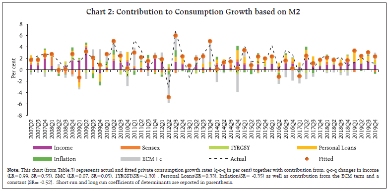
Next, we focus on the two best models (named as M1 and M2) out of 12 models, i.e., the models with the lowest RMSE, and use these to estimate the contribution of each factor in growth of private consumption in the short run. The results are furnished below in Table 3. As per the model results (Table 3), income and wealth together account for an average 50 per cent share in the growth of private consumption in the short-run. The cyclical factors, including credit channel (interest rate and loans), contribute the remaining share to private consumption growth during the sample period (Charts 1 and 2). Asymmetric effect of interest rates The results of models to capture asymmetric effects of interest rate on private consumption are presented in Table 4. Although direction of the impact remains same (negative influence) which is on the expected lines, the degree of impact varies signifying an asymmetric impact of interest rate on private consumption. Additionally, the Wald test suggests that the coefficients of IRt+ and IRt- are significantly different from each other. The results indicate that higher interest rates weigh more on private consumption than an equivalent easing of interest rates, which suggests that monetary policy may be more effective in containing private consumption and domestic demand relative to boosting the same. | Table 3: Short run dynamics of the best two models | | Variable | M1 | M2 | | | Coefficients | | Income | 0.41*** | 0.55*** | | | (13.81) | (15.63) | | Sensex | 0.03*** | | | | (4.15) | | | SMC | | 0.05*** | | | | (8.22) | | WALR | -1.38*** | | | | (-6.22) | | | 1YRGSY | | -1.30*** | | | | (-5.03) | | Personal Loans | 0.29*** | 0.33*** | | | (10.24) | (8.06) | | Government Debt | 0.30*** | | | | (6.80) | | | Inflation | -0.28*** | -0.35*** | | | (-3.32) | (-4.85) | | ECT | -0.48** | -0.52*** | | | (-10.16) | (-10.75) | | R2 | 0.72 | 0.71 | | Prob (J-statistic) | 0.98 | 0.94 | | Q-statistic (upto 5 lags) (p-value) | 0.24 | 0.48 | | Note: ***, **, * represent statistical significance at less than 1, 5 and 10 per cent levels, respectively. Figures in parentheses are t-statistic. |

| Table 4: GMM estimation for asymmetric test | | Variables | Model 1 | Model 2 | Model 3 | Model 4 | | Income | 0.57*** | 0.57*** | 0.54*** | 0.56*** | | Sensex | 0.01** | 0.03*** | 0.03*** | 0.03*** | | WALR– | 1.19*** | 0.72*** | | | | WALR+ | -4.40*** | -4.34*** | | | | 1YRGSY- | | | 1.22*** | | | 1YRGSY+ | | | -4.31*** | | | 10YRGSY– | | | | 2.25*** | | 10YRGSY+ | | | | -5.36*** | | Government Debt | 0.07* | 0.13*** | 0.19*** | 0.22*** | | Personal loans | | 0.04** | 0.05* | | | Inflation | -0.33*** | -0.39*** | -0.43*** | -0.46*** | | ECT | -0.59*** | -0.53*** | -0.49*** | -0.53*** | | Wald chi2 | 65.48*** | 58.49*** | 111.90*** | 62.09*** | | Note: ***, **, * represent statistical significance at less than 1, 5 and 10 per cent levels, respectively. | 5. Concluding observations Given the dominant contribution of private consumption to aggregate demand and growth, we empirically examine the macroeconomic drivers of private consumption over short and long horizons in India. It is found that there exists a long-run co-integrating relationship between real private consumption, income and wealth, with income elasticity close to unity pointing towards a strong co-movement of consumption and income over time. In the short-run, interest rate, consumer indebtedness, government indebtedness, inflation and uncertainty also impact private consumption. The interest rate channel signifies the role of monetary policy to manage domestic demand and inflation. Furthermore, the impact of interest rate is found to be asymmetric, with monetary policy more effective in containing private consumption than boosting the same. Bank credit boosts private consumption through easing liquidity and financial constraints. Government indebtedness also shores up private consumption through social transfers and subsidies boosting purchasing power of households and capex spending boosting private investment and incomes. High inflation reduces purchasing power and consequently, it has an adverse impact on private consumption and overall growth. In the short run, as the empirical analysis shows, a bouquet of factors drive private consumption which is the mainstay of aggregate demand and an ongoing comprehensive evaluation of all such factors is essential to arrive at a realistic assessment of the evolving domestic demand conditions. References: Aiolfi, M., & Favero, C. A. (2005). Model uncertainty, thick modelling and the predictability of stock returns. Journal of Forecasting, 24(4), 233-254. Aizenman, J., Cheung, Y. W., & Ito, H. (2019). The interest rate effect on private saving: Alternative evidence from the household survey data in Japan. Journal of the Japanese and International Economies, 52, 14-36. Ando, A., & Modigliani, F. (1963). The life cycle hypothesis of saving: aggregate implications and tests. American Economic Review, 53(1), 55–84. Apergis, N., & Miller, S. M. (2006). Consumption asymmetry and the stock market: empirical evidence. Economic Letters, 93(3), 337–342. Athukorala, P. C., & Sen, K. (2004). The Determinants of Private Saving in India. World Development, 32(3), 491-503. Auclert, A. (2019). Monetary Policy and the Redistribution Channel. American Economic Review, 109(6), 2333-2367. Ayunasta, P., Setiaji, B., & Hakim, L. (2020). Debt and consumption in Indonesia: Ricardian equivalence approach. Issues on Inclusive Growth in Developing Countries, 1(1), 49-60. Baker, S. R. (2018). Debt and the response to household income shocks: Validation and application of linked financial account data. Journal of Political Economy, 126(4), 1504-1557. Benjamin, J. D., Chinloy, P., & Jud, G. D. (2004). Real estate versus financial wealth in consumption. The Journal of Real Estate Finance and Economics, 29(3), 341–354. Boskin, M. J. (1978). Taxation, saving and the rate of interest. Journal Political Economy, 86(2), 3–27. Bostic, R., Gabriel, S., & Painter, G. (2009). Housing wealth, financial wealth, and consumption: new evidence from micro data. Regional Science and Urban Economics, 39(1), 79–89. Bunn, P., Le Roux, J., Reinold, K., & Surico, P. (2018). The consumption response to positive and negative income shocks. Journal of Monetary Economics, 96, 1-15. Cagan, P. (1956). The Monetary Dynamics of Hyperinflation. In Friedman M. (Ed.), Studies in the Quantity Theory of Money. University of Chicago Press: Chicago, USA. Carroll, C. D., & Kimball, M. S. (1996). On the concavity of the consumption function. Econometrica, 64(4), 981–992. Case, K. E., Quigley, J. M., & Shiller, R. J. (2013). Wealth effects revisited 1975–2012. Critical Finance Review, 2(1), 101–128. Cho, D., & Rhee, D. E. (2013). Nonlinear effects of government debt on private consumption: Evidence from OECD countries. Economics Letters, 121(3), 504-507. Christelis, D., Georgarakos, D., Jappelli, T., Pistaferri, L., & Van Rooij, M. (2019). Asymmetric consumption effects of transitory income shocks. The Economic Journal, 129(622), 2321-2350. D’Erasmo, P., Mendoza, E. G., & Zhang, J. (2017). What is a Sustainable Public Debt? American Economic Review, 107(6), 1611–1641. Deaton, A., & Paxson, C. (1994). Saving, growth, and aging in Taiwan. In R. F. Engle & C. W. Granger (Eds.), Long-run Economic Relationships: Readings in Cointegration (pp. 163-195). Oxford University Press. Debelle, G., & Lamont, O. (1997). Relative price variability and inflation: Evidence from US cities. Journal of Political Economy, 105(1), 132-152. Dietz, R. D., & Haurin, D. R. (2003). The social and private micro-level consequences of homeownership. Journal of Urban Economics, 54(3), 401-450. Dustmann, C., Fasani, F., & Speciale, B. (2017). Illegal migration and consumption behavior of immigrant households. The Economic Journal, 127(600), 1543-1578. Edelberg, W., Guerrieri, V., & Sill, K. E. (2007). Retail prices during a housing boom: identifying supply-side distortions using census micro data. The Review of Economics and Statistics, 89(1), 10–23. Engelhardt, G. V. (1996). Consumption, down payments, and liquidity constraints. Journal of Money, Credit and Banking, 28(2), 255–271. Fagereng, A., Guiso, L., Malacrino, D., & Pistaferri, L. (2019). Heterogeneity and persistence in returns to wealth. Econometrica, 87(6), 2107-2144. Feldstein, M. S. (1974). Social security, induced retirement, and aggregate capital accumulation. Journal of Political Economy, 82(5), 905-926. Ferguson, R. W., & Peters, M. (1995). The effect of real estate wealth on household consumption in the presence of credit constraints. Real Estate Economics, 23(4), 417-435. Fisher, J. D. (2006). The dynamic effects of neutral and investment-specific technology shocks. Journal of Political Economy, 114(3), 413-451. Flavin, M. A. (1981). The adjustment of consumption to changing expectations about future income. Journal of Political Economy, 89(5), 974–1009. Fratzscher, M., & Juvenal, L. (2018). News shocks, sovereign risk, and sovereign debt maturity. Journal of International Economics, 112, 109-134. Fuster, L., Llena-Nozal, A., & Zafar, B. (2021). Housing wealth, employment, and the age of entrepreneurs. Journal of Monetary Economics, 117, 1068-1092. Gabaix, X. (2011). The granular origins of aggregate fluctuations. Econometrica, 79(3), 733-772. Gali, J. (1994). Government size and macroeconomic stability. European Economic Review, 38(1), 117–132. Geanakoplos, J., Magill, M. J., & Quinzii, M. (2004). Demography and the long-run predictability of the stock market. Journal of Financial Economics, 73(3), 401–430. Gertler, M., & Grinols, E. (1982). Monetarism, inflation, and the business cycle: Comment. Journal of Money, Credit and Banking, 14(4), 602–607. Gianonne, D., Lenza, M., & Primiceri, G. E. (2017). Credit shocks and aggregate fluctuations in an economy with production heterogeneity. Review of Economic Studies, 84(2), 792–832. Giglio, S., Maggiori, M., & Stroebel, J. (2020). Five facts about beliefs and portfolios. Journal of Economic Perspectives, 34(3), 94-121. Goel, R., & Saunoris, J. W. (2018). Stock markets, consumption, and real activity: a cross-country analysis. Journal of International Financial Markets, Institutions and Money, 54, 23-49. Greenwood, J., Hercowitz, Z., & Huffman, G. (1988). Investment, capacity utilization, and the real business cycle. American Economic Review, 78(3), 402–417. Hall, R. E. (1978). Stochastic implications of the life cycle-permanent income hypothesis: theory and evidence. Journal of Political Economy, 86(6), 971–987. Hamilton, J.D., Perez-Quiros, G. (1996). What do the leading indicators lead? Journal of Business, 69(1), 27–49. Hanna, S., Fan, Q., Kabukcuoglu, Z., Kalcheva, K., Li, L., Metrick, A., & Yildirim, Y. (2018). House money: the effects of the 2008 mortgage crisis on consumer behavior. The Review of Financial Studies, 31(6), 2343–2380. Himmelberg, C., Mayer, C., & Sinai, T. (2005). Assessing high house prices: bubbles, fundamentals, and misperceptions. Journal of Economic Perspectives, 19(4), 67–92. Huggett, M. (1993). The risk-free rate in heterogeneous-agent incomplete-insurance economies. Journal of Economic Dynamics and Control, 17(5-6), 953–969. Jappelli, T., & Pistaferri, L. (2014). Does consumption inequality track income inequality in Italy? The Economic Journal, 124(581), 1296-1316. Johansson, A., & Ronnqvist, M. (2015). Financial sophistication and wealth accumulation: evidence from Swedish lottery players. Journal of Banking & Finance, 56, 12-23. Kaplan, G., & Violante, G. L. (2014). A model of the consumption response to fiscal stimulus payments. Econometrica, 82(4), 1199–1239. Kaplanis, I. (2021). Housing market activity, unemployment, and consumption asymmetry: Evidence from Greece. Journal of Housing Economics, 52, 101817. Karatheodoris, A., & Katrakilidis, C. (2012). Consumption and leisure: nonlinear dynamics in an OLG growth model with endogenous time allocation. Journal of Macroeconomics, 34(1), 189–207. Keller, W., & Shiue, C. H. (2018). The paradox of power: Understanding fiscal capacity in Imperial China and absolutist regimes. Journal of Economic History, 78(3), 756-791. Kim, K., & Roubini, N. (2008). Twin deficit or twin divergence? Fiscal policy, current account, and real exchange rate in the US. Journal of International Economics, 74(2), 362-383. Kodila-Tedika, O., Rindermann, H., Sacko, A., & Sonedjou, I. (2019). Sonedjou I (2019). Pre-colonial institutions and modern economic growth: the case of West Africa. Journal of Institutional Economics, 15(2), 263-289. Kumhof, M., Laxton, D., & Muir, D. (2012). The global integrated monetary and fiscal model (GIMF): Theoretical structure. Journal of Economic Dynamics and Control, 34(1), 1-45. Leeper, E. M. (1991). Equilibria under “active” and “passive” monetary and fiscal policies. Journal of Monetary Economics, 27(1), 129–147. Leeper, E. M., Sims, C. A. & Zha, T. (1996). What does monetary policy do? Brookings Papers on Economic Activity, 2, 1–78. Lettau, M., & Ludvigson, S. C. (2019). Shocks and crashes. The Review of Financial Studies, 32(6), 2304-2341. Li, K., Zhang, F., & Zhao, L. (2021). Stock market volatility, household consumption, and uncertainty shocks. International Review of Financial Analysis, 73, 101674. Liu, Z., & Sercu, P. (2017). Asset pricing when the representative investor cares about beliefs’ impact on her future wealth. Journal of Financial Economics, 126(3), 556-578. Lucas Jr, R. E. (1976). Econometric policy evaluation: A critique. Carnegie-Rochester Conference Series on Public Policy, 1, 19–46. Malmendier, U., & Nagel, S. (2011). Depression babies: do macroeconomic experiences affect risk taking? Quarterly Journal of Economics, 126(1), 373–416. Modigliani, F., & Brumberg, R. (1954). Utility analysis and the consumption function: An interpretation of cross-section data. Post-Keynesian Economics, 388–436. Mulligan, C. B., & Sala-i-Martin, X. (1999). Social security in theory and practice (II): Efficiency theories, narrative theories, and implications for reform. NBER Working Paper Series, 7118. Müller, K., Fuchs-Schündeln, N., Şahinb, A., & Içilc, S. (2019). Labor market policies and capital taxation in a labor market with search frictions. Journal of Monetary Economics, 107, 91-106. Nelson, C. R., & Plosser, C. I. (1982). Trends and random walks in macroeconmic time series: Some evidence and implications. Journal of Monetary Economics, 10(2), 139–162. Okun, A. M. (1962). Potential GNP: its measurement and significance. Proceedings of the Business and Economic Statistics Section, American Statistical Association, 98–104. Pagano, M., & Bianco, M. (2020). Sovereign risk, fiscal policy, and macroeconomic stability. Journal of Monetary Economics, 115, 114-129. Parker, J. A. (1999). The reaction of household consumption to predictable changes in social security taxes. American Economic Review, 89(4), 959–973. Pistaferri, L. (2016). Handbook of macroeconomics, 2A, 2305-2410. Poterba, J. M. (1988). Comment on “Investment and Tobin’s Q.” Journal of Political Economy, 96(6), 1302-1304. Ramey, V. A. (2016). Macroeconomic shocks and their propagation. Journal of Economic Literature, 54(1), 87-144. Reis, R. (2013). The mystique surrounding the central bank’s balance sheet, applied to the European crisis. Journal of Economic Perspectives, 27(3), 3-28. Romer, C. D., & Romer, D. H. (1989). Does monetary policy matter? A new test in the spirit of Friedman and Schwartz. NBER Macroeconomics Annual, 4, 121-170. Sims, C. A. (1992). Interpreting the macroeconomic time series facts: The effects of monetary policy. European Economic Review, 36(5), 975-1000. Stock, J. H., & Watson, M. W. (2002). Macroeconomic forecasting using diffusion indexes. Journal of Business & Economic Statistics, 20(2), 147-162. Summers, L. H. (2014). U.S. economic prospects: Secular stagnation, hysteresis, and the zero lower bound. Business Economics, 49(2), 65-73. Taylor, J. B. (1993). Discretion versus policy rules in practice. Carnegie-Rochester Conference Series on Public Policy, 39, 195–214. Woodford M (2012). Inflation targeting and financial stability. NBER Working Paper Series, 17967. Yao, F., Wei, J., & Yu, J. (2018). Fiscal deficit and household consumption in China: Evidence from a provincial panel analysis. China Economic Review, 50, 110-124. Zeldes, S. P. (1989). Optimal consumption with stochastic income: Deviations from certainty equivalence. The Quarterly Journal of Economics, 104(2), 275-298. Zhang, S., Wang, P., & Wang, J. The effects of social security on private consumption: Evidence from China. Journal of Comparative Economics, 48(3), 528-547.
Appendix | Table A1: List of Variables | | Category | Variable | Sources | | Consumption | Private consumption | National Statistical Office (NSO) | | Income | Personal Disposable Income | NSO | | Wealth | Sensex | BSE Limited | | Stock Market Capitalization (SMC) | BSE Limited | | Interest rate | Weighted average call money rate (WACR) | RBI | | Weighted average money lending rate (WALR) on outstanding rupee loans of scheduled commercial banks | RBI | | 10-year government securities yield (10YGSY) | RBI | | 1-year government sec yield (1YRGSY) | RBI | | Consumer indebtedness | Personal Loans | RBI | | Government indebtedness | Central Government Debt | MoF | | Uncertainty | Uncertainty Index | www.policyuncertainity.com | | Crude Oil Price | MoPNG | | Inflation | Inflation based on PFCE | NSO | | Demographic | Old-age-dependency Ratio | World Bank |
| Table A2: Summary Statistics | | Variables | Units | Mean | Std. Dev. | Minimum | Maximum | | Consumption | % yoy | 1.87 | 1.69 | -3.14 | 7.11 | | Income | % yoy | 3.15 | 0.85 | 1.92 | 7.07 | | Sensex | % yoy | 3.74 | 9.62 | -32.72 | 36.90 | | SMC | % yoy | 4.88 | 11.44 | -34.75 | 40.10 | | WACR | % pa | 6.50 | 1.60 | 3.20 | 9.80 | | WALR | % pa | 11.60 | 0.80 | 10.10 | 13.10 | | 10YGSY | % pa | 7.60 | 0.70 | 5.40 | 8.90 | | 1YRGSY | % pa | 7.00 | 1.20 | 4.20 | 9.40 | | Personal Loans | % yoy | 3.82 | 1.98 | -1.87 | 11.76 | | Government Debt | % yoy | 2.83 | 1.26 | -0.08 | 7.13 | | Uncertainty Index | Index | 95.20 | 46.80 | 34.50 | 234.50 | | Crude Oil Price | (USD/barrel) | 73.10 | 25.00 | 31.70 | 118.80 | | Inflation | % yoy | 1.35 | 0.93 | -0.58 | 4.10 | | Old-age-dependency Ratio | % | 7.99 | 0.47 | 7.37 | 9.77 |
| Table A3: Unit Root Tests | | | ADF | Phillips-Perron | | Variable | Level | Diff | Level | Diff | | Consumption | -1.56 | -10.73*** | -1.96 | -14.55*** | | Income | -0.49 | -6.65*** | -2.56* | -6.78*** | | Sensex | -2.99 | -5.63*** | -2.78* | -5.63*** | | SMC | -2.81 | -5.25*** | -2.67* | -5.25*** | | WACR | -2.72 | -7.29*** | -2.48 | -7.29*** | | WALR | -3.15 | -6.91*** | -2.85* | -6.91*** | | 10YRGSY | -2.79 | -6.61*** | -2.67* | -6.61*** | | 1YRGSY | -2.51 | -6.38*** | -2.31 | -6.38*** | | Personal Loans | 0.19 | -5.32*** | -0.83 | -5.32*** | | Government Debt | -0.12 | -8.23*** | -0.67 | -8.23*** | | Uncertainty Index | -2.56 | -7.37*** | -2.26 | -7.37*** | | Crude Oil Price | -1.69 | -5.83*** | -1.24 | -5.83*** | | Inflation | -0.37 | -5.74*** | -0.38 | -5.74*** | | Old-age-dependency Ratio | -0.50 | -7.39*** | 8.30 | -7.39*** | | Note: ***, ** and * represent statistical significance at 1, 5 and 10 per cent levels, respectively. The lag length in the ADF tests was chosen based on Schwarz Bayesian Criterion (SBC). |
| Table A4: Correlation Table | | Variables | Lag | | 0 | 1 | 2 | 3 | 4 | | Income | 0.99*** | 0.99*** | 0.99*** | 0.99*** | 0.99*** | | Sensex | 0.96*** | 0.96*** | 0.96*** | 0.96*** | 0.95*** | | SMC | 0.96*** | 0.96*** | 0.96*** | 0.96*** | 0.96*** | | WACR | 0.15 | 0.12 | 0.09 | 0.08 | 0.04 | | WALR | -0.77*** | -0.76*** | -0.75*** | -0.74*** | -0.73*** | | 10YGSY | 0.04 | -0.02 | -0.09 | -0.14 | -0.19* | | 1YGSY | 0.15 | 0.13 | 0.09 | 0.06 | 0.02 | | Personal Loans | 0.97*** | 0.97*** | 0.97*** | 0.97*** | 0.97*** | | Government Debt | 0.99*** | 0.99*** | 0.99*** | 0.99*** | 0.99*** | | Uncertainty Index | -0.08 | -0.07 | -0.08 | -0.1 | -0.13 | | Crude Oil Price | -0.04 | -0.07 | -0.11 | -0.16 | -0.20* | | Inflation | 0.95*** | 0.97*** | 0.97*** | 0.97*** | 0.95*** | | Note: ***, ** and * represent statistical significance at 1, 5 and 10 per cent levels, respectively. |
| Table A5: Determinants of Consumption | | Variables | Tested sign | Expected sign | | Income | [+] | [+] | | Sensex | [+] | [+] | | SMC | [+] | [+] | | WACR | [-] | [-] | | WALR | [-] | [-] | | 10YRGSY | [-] | [-] | | 1YRGSY | [-] | [-] | | Personal Loans | [+] | [+] | | Government Debt | [+] | Ambiguous | | Uncertainty Index | [-] | [-] | | Crude Oil Price | [-] | [-] | | Inflation | [-] | [-] | | Old-age-dependency Ratio | [+] | [+] | | Note: This table represents the summary of variables included in the benchmark model. The estimated preliminary sign in the benchmark ECM for each variable separately is reported in the third column. |
| Table A6: Granger Causality Test Results | | Null Hypothesis: | F-Statistic | Prob. | | Income does not Granger Cause Consumption | 1.94 | 0.07 | | Income (-1) does not Granger Cause Consumption | 4.21 | 0.00 | | Sensex does not Granger Cause Consumption | 0.74 | 0.60 | | Sensex (-1) does not Granger Cause Consumption | 1.05 | 0.15 | | Sensex (-2) does not Granger Cause Consumption | 2.56 | 0.08 | | Sensex (-3) does not Granger Cause Consumption | 3.10 | 0.02 | | SMC does not Granger Cause Consumption | 0.70 | 0.56 | | SMC (-1) does not Granger Cause Consumption | 0.99 | 0.18 | | SMC (-2) does not Granger Cause Consumption | 1.36 | 0.11 | | SMC (-3) does not Granger Cause Consumption | 2.63 | 0.03 | | WACR does not Granger Cause Consumption | 3.15 | 0.02 | | WACR (-1) does not Granger Cause Consumption | 3.29 | 0.01 | | WALR does not Granger Cause Consumption | 4.13 | 0.00 | | WALR (-1) does not Granger Cause Consumption | 3.98 | 0.01 | | 10YRGSY does not Granger Cause Consumption | 3.78 | 0.01 | | 10YRGSY (-1) does not Granger Cause Consumption | 4.74 | 0.00 | | 1YRGSY securities do not Granger Cause Consumption | 3.18 | 0.02 | | 1YRGSY (-1) does not Granger Cause Consumption | 4.41 | 0.00 | | Central Government Debt does not Granger Cause Consumption | 0.39 | 0.86 | | Central Government Debt (-1) does not Granger Cause Consumption | 0.87 | 0.20 | | Central Government Debt (-2) does not Granger Cause Consumption | 1.47 | 0.14 | | Central Government Debt (-3) does not Granger Cause Consumption | 2.08 | 0.04 | | Personal Loans do not Granger Cause Consumption | 0.99 | 0.43 | | Personal Loans (-1) does not Granger Cause Consumption | 1.97 | 0.07 | | Personal Loans (-2) does not Granger Cause Consumption | 2.52 | 0.05 | | Uncertainty index does not Granger Cause Consumption | 0.70 | 0.22 | | Uncertainty index (-1) does not Granger Cause Consumption | 0.60 | 0.25 | | Uncertainty index (-2) does not Granger Cause Consumption | 1.62 | 0.13 | | Uncertainty index (-3) does not Granger Cause Consumption | 2.34 | 0.07 | | Crude oil price does not Granger Cause Consumption | 0.92 | 0.48 | | Crude oil price (-1) does not Granger Cause Consumption | 0.28 | 0.92 | | Inflation does not Granger Cause Consumption | 3.87 | 0.01 | | Inflation (-1) does not Granger Cause Consumption | 4.44 | 0.00 | | Old-age-dependency ratio does not Granger Cause Consumption | 0.90 | 0.49 | | Old-age-dependency ratio (-1) does not Granger Cause Consumption | 1.50 | 0.21 |
| Table A7: Short-run dynamics of the final selected models | | Variables | EQ1# | EQ2# | EQ3 | EQ4 | EQ5 | EQ6 | EQ7 | EQ8 | EQ9 | EQ10 | EQ11 | EQ12 | | Income | 0.41*** | 0.55*** | 0.49** | 0.64** | 0.46** | 0.59** | 0.64** | 0.41** | 0.57** | 0.43** | 0.45** | 0.40** | | Sensex | 0.03*** | | 0.01** | 0.02** | 0.02** | 0.03* | 0.02** | 0.04** | 0.05** | | | | | SMC | | 0.05*** | | | | | | | | 0.02** | 0.02** | 0.03** | | WALR | -1.38*** | | -1.22** | | | | | | | -1.29** | | | | 10YRGSY | | | | -1.64** | -1.31** | -1.40** | | | | | -1.32** | | | 1YRGSY | | -1.30*** | | | | | -1.97** | -1.40** | -1.80** | | | -1.46** | | Personal Loans | 0.29*** | 0.33*** | 0.37** | 0.37** | 0.38** | 0.43** | 0.38** | 0.41** | 0.46** | 0.35** | 0.34** | 0.36** | | Government Debt | 0.30*** | | 0.22** | | 0.23** | | | 0.25** | | 0.25** | 0.24** | 0.27** | | Uncertainty Index | | | -0.01** | -0.01** | | | -0.01** | | | | | | | Inflation | -0.28*** | -0.35*** | | | -0.19** | -0.20** | | -0.30** | -0.30** | -0.27** | -0.20** | -0.25** | | ECT | -0.48** | -0.52*** | -0.48** | -0.47** | -0.49** | -0.50** | -0.48** | -0.50** | -0.50** | -0.50** | -0.49** | -0.49** | | R2 | 0.72 | 0.71 | 0.65 | 0.66 | 0.71 | 0.68 | 0.64 | 0.71 | 0.67 | 0.68 | 0.69 | 0.70 | | Prob (J-statistic) | 0.98 | 0.94 | 0.98 | 0.93 | 0.97 | 0.92 | 0.98 | 0.99 | 0.98 | 0.98 | 0.98 | 0.98 | Note: ***, **, * represent statistical significance at less than 1, 5 and 10 per cent levels, respectively.
#: The reported two best models in Table 3: --are based on EQ1 and EQ2. |
|