by Deba Prasad Rath, G V Nadhanael and Shobhit Goel^{^}

This article analyses the extent of forward-looking information contained in various sources of information about the trajectory of crude oil prices. Our results show that qualitative information, such as the forecasts available from the Survey of Professional Forecasters (SPF), tends to outperform the futures prices. The forecast accuracy of futures prices improves once we account for trends in real economic activity, such as capacity utilisation in key oil consumer economies. Also, our results indicate that forecast accuracy tends to improve for all forecasts methods including, naïve forecast, futures prices, adjusted futures prices, SPF, and those provided by US-Energy Information Administration (EIA), when the futures trajectory is lower than the current price (backwardation), highlighting the role of market conditions in shaping forecast accuracy.

I. Introduction

Understanding the dynamics of crude oil markets and assessing the likely trajectory of prices in the future are important for policymakers for a number of reasons. For central banks, especially those with a mandate for inflation targeting, making reliable and robust inflation forecasts is paramount for both ‘anchoring’ inflation expectations and also for its own ‘credibility’ (Baumeister & Kilian, 2014b; Garga et al., 2022). Given India’s large share of food and fuel in overall consumption, coming up with the best possible forecasts for these supply-side drivers of inflation is critical. In India, crude oil prices significantly impact inflation through their direct and indirect effects on prices of goods and services that use crude oil and its products as inputs (John et al., 2020). Given this, crude oil price outlook is an essential input for the Monetary Policy Committee’s (MPC’s) deliberations on inflation projections.

Although the dependency of economic activity on crude oil has fallen steadily over the last thirty years with a shift towards cleaner and renewable sources of energy, crude oil continues to play a critical role in the economy (Blanchard & Gali, 2007; Pagano & Pisani, 2009). Crude oil is crucial for producing a wide range of goods and services, especially transportation. Higher oil prices raise the cost of inputs, and when they are passed through to output prices, they contribute to inflation. If these cost increases can’t be passed on to consumers, profit margins of firms could be impacted, denting the growth and investment outlook. Conversely, a drop in oil prices can stimulate economic growth by reducing production costs and encouraging production (Ahmad et al., 2022; da Silva Souza & de Mattos, 2023; Sadath & Acharya, 2021). If administered prices suppress the inflation impact of high oil prices, it could lead to fiscal strain, as the subsidy burden would increase. Further, higher oil prices widen the current account deficit (CAD), given the high import dependency. As crude oil prices influence a host of these macroeconomic variables, their forecasts play an essential role in setting the outlook for these variables.

This article examines the alternate sources of information - including naïve forecasts¹, futures prices², adjusted futures prices, US Energy Information Administration (EIA) and the Survey of Professional Forecasters (SPF) of the Reserve Bank of India (RBI) forecast for crude oil prices - on the future trajectory of oil prices and attempts to assess their usefulness for arriving at a realistic outlook for the oil price trajectory. Specifically, the article contributes to the literature by providing a comprehensive analysis of various sources of information on oil price outlook and comparing their forecast accuracy. Also, our methodology of adjusting for demand conditions adds a different dimension to using oil prices for forecasting. Moreover, this article also compares the forecast performance across different market conditions as characterized by the market conditions, i.e., whether the futures prices are higher or lower than current prices.

We first provide an overview of the forecasting methods used to project oil prices. Specifically, we analyse the assessment of the US EIA and the SPF of the RBI. Thereafter, we analyse the extent to which forward-looking information is contained in the oil futures prices and empirically assess whether explicitly accounting for demand factors can help improve the predictive power of futures prices. Thereafter, we look at the forecast performance of these alternate sources across different market conditions and their policy implications.

II. Approaches to Forecasting Oil Prices

The oil price forecasting methods can be broadly classified into two categories. The first category, qualitative forecasting, uses traditional methods that rely on estimates provided by professional forecasters and industry experts, focusing on assessing the impact of infrequent events such as wars and natural disasters on oil prices (Alquist et al., 2011). More recently, qualitative information is also analysed in a more structured manner. Machine learning and Artificial Intelligence (AI)-based techniques³ which leverage on advanced computational tools to analyse vast amounts of information and extract valuable insights for predicting oil prices are also being increasingly used (Bashiri et al., 2013).

On the other hand, the second category, quantitative forecasting, relies on econometric methods that employ statistical techniques to model and predict oil prices. Time series models play a crucial role in this category by utilising historical data to identify systematic patterns, such as autocorrelation, to make projections for crude oil prices (Frey et al., 2009). They are particularly well-suited for crude oil prices, as the data exhibits recurring patterns. Additionally, financial market models explore the intricate relationship between spot and futures prices, shedding light on how they influence one another. Meanwhile, structural models delve into the impact of specific economic factors and the behaviour of economic agents on the future spot crude oil prices, offering valuable insights into the underlying mechanisms driving price movements. Furthermore, non-standard models such as Artificial Neural Networks (ANN) and Support Vector Machines (SVM) provide alternative approaches that leverage advanced computational techniques to enhance oil price forecasts beyond the capabilities of traditional econometric methods. These models represent a dynamic and evolving field in research on oil price forecasting.

Traditional Qualitative Forecasts

Estimates provided by professional forecasters and industry experts can be considered under the category of qualitative forecasts as they often are based on the qualitative judgments of the forecasters who employ their overall understanding and experience to provide a forecast, especially in case of estimating the impact of infrequent events such as wars and natural disasters.⁴ We look at two such sources in detail.

First is the information from the U.S. Energy Information Administration (EIA), which provides monthly forecasts for up to 2 years ahead. The EIA forecast is based on analysts’ judgments using different variables as guides. These include (1) price forecasts from the pooled and regression models, (2) the previous month’s price forecast, and (3) futures prices. The pooling model utilises an average of five separate models based on historical economic and oil market activity data utilizing different quantitative techniques. These include a vector autoregressive (VAR) model, a model based on the spread between oil futures prices and the spot price of oil, a model using non-oil industrial commodity prices, a model with a time-varying parameter representing the relationship between the spreads between the U.S spot prices of gasoline and heating oil and the spot price of crude oil, and a model based on the cumulative change in U.S. crude oil inventory levels. Another input utilised by EIA is a linear regression model based on inputs from the Short-term Economic Outlook (STEO) global oil market forecast. It considers month-to-month changes in US petroleum inventory levels, global GDP, and petroleum inventory levels in Organisation for Economic Co-operation and Development (OECD) countries. As inventory levels can reflect short-term market imbalances, they are seen to capture better the cumulative effect of demand and supply side factors (EIA US, 2020).

The second source we analyse in detail is the Reserve Bank of India (RBI)’s Survey of Professional Forecasters (SPF) which provides aggregated results from a bi-monthly survey of professional forecasters. The survey elucidates the participants’ forecast for crude oil price for the coming quarters. The SPF was initiated as a quarterly survey in the second quarter of 2007-08, and the crude price forecast has been published since 2008-09:Q4 round (7th round), which provides a forecast for 2009-10:Q1. In order to align with the monetary policy cycle, the SPF was shifted to a bi-monthly frequency from the 28th round. The SPF in a way is also a combination forecast as it takes the median forecast price predicted by different professional forecasters all of whom may have used different forecasting techniques and models.

Structural Models

In structural models, the crude oil price forecast is modelled to be dependent on a group of fundamental economic variables, with standard explanatory variables being OPEC output commitments, inventory levels in major oil consumers, oil consumption and production of major economies, and other macro-economic variables like GDP growth rate, interest rate, exchange rate, and other commodity prices. Yang et al., (2002) utilises an error correction model (ECM) to estimate the demand equation and related elasticities. It includes the impact of income effect and resultant demand shift for crude oil and supply side structure by including OPEC market structure and its attempt at cartelization. Further, simple models to forecast short-term WTI crude oil spot prices by using OECD petroleum inventories have been attempted in literature (Merino & Alvaro Ortiz, 2005; Ye et al., 2002, 2005). Merino & Alvaro Ortiz (2005) attempts to estimate if other variables, including the oil market, financial market, and commodity prices, apart from inventory levels, improve the original model, but that non-oil market variables do not improve the model and only oil market variables like speculation and OPEC spare capacity improve the overall explanatory power. Vector autoregressive (VAR) and Structural VAR (SVAR) models to forecast crude oil prices have gained significant attention in the literature, as these models allow for endogenizing the price of oil instead of assuming exogenous oil prices. Kilian (2009) creates a global real economic activity index, which decomposes the oil price shocks into three components: oil supply shock, global demand shock for all industrial activities, and a specific demand shock for oil. Baumeister & Kilian (2012) finds that the real-time forecasts made using the VAR model based on global oil market variables are more accurate than the no-change forecast and even Autoregressive (AR), Autoregressive moving-average (ARMA), and futures prices-based forecast, especially for horizons up to one year. VAR models can also be used to evaluate the sensitivity of the baseline forecast to alternative forecast scenarios, which may involve shocks to demand and supply of oil (Baumeister & Kilian, 2014a). Wang et al., (2015) employed a model which included variables such as futures price, global oil production, global economic activity, and changes in oil inventory, among other variables, to forecast crude oil prices. They found the model to have superior performance than a no-change model.

Futures Prices

Another category of quantitative forecasting model is based on financial market data. These models investigate if futures prices can be used to obtain unbiased and efficient forecasts of crude oil prices. If the crude oil futures markets are efficient, then futures prices should reflect all presently available information which may drive the crude oil prices in future, making them a helpful tool for predicting crude oil prices (Gulen, 1998). Futures prices may be useful in predicting crude oil prices, particularly in the short term. On an evaluation of the predictive accuracy of 1, 3, 6, 9, and 12 months ahead crude oil futures prices for forecasting the crude oil prices, Abosedra et al., (2004) finds that although futures prices and naïve forecasts are unbiased at all forecast horizons, only the 1 and 12 month ahead futures prices based forecasts outperform the naïve forecast. Therefore, given the limitations of using futures prices alone to predict crude oil prices, even in an efficient market, it is important to consider other factors that can affect crude oil prices, such as macroeconomic conditions, changes in production and consumption patterns, and geopolitical events. Furthermore, sudden supply disturbances, such as any major geo-political event, can adversely affect the predictive accuracy of futures prices as futures prices also respond to news about supply-side developments like spot prices. Although Chinn et al., (2005) found that futures prices are unbiased predictors of crude oil prices and do slightly outperform time series and random walk models in predicting crude oil prices, they have limited predictive capacity. Recent literature, however, find that futures price-based forecasts can produce reasonable forecasts, especially for short and medium-term periods. To improve forecast performance, some have argued for a model that imposes very little structure on the relationship between spot and futures prices; others have proposed the usage of the term structure (Bredin et al., 2021; Chu et al., 2022).

Adjusted Futures Prices

Attempts have been made to correct the biases in futures prices to improve their forecast performance. Pagano and Pisani (2009) find that the futures prices are not unbiased predictors of crude oil prices, as the mean forecast error for each forecast horizon is significantly negative, ranging from US$ 0.73, US$ 1.89, and US$ 4.37 for 3-, 6- and 12-month horizon. They used a monthly average of futures prices for West Texas Intermediate (WTI) grade of crude oil for different horizons. They further investigated whether business cycle phases explained the forecast errors and regressed the error on the US capacity utilisation data released by the Federal Reserve every month. They found that forecast errors and capacity utilisation are negatively related. The slope coefficient increases in magnitude with the increase in forecast horizon and is also statistically significant from the 4-month horizon onwards. Using an out-of-sample forecasting exercise, they found that adjusted forecasts are more precise than those obtained with unadjusted futures, random walk, or futures adjusted for a constant value, particularly at longer horizons (greater than six months).

Since our objective is to assess the relative forecast performance of various sources of information, we also attempt to generate an adjusted futures price series. Following the methodology utilized by Pagano et.al., (2009), we examine whether the futures prices are an unbiased estimator of crude oil prices and then try to adjust the futures prices with real sector indicators. Our approach, however, differs on specific accounts. We utilise the average quarterly price to generate and evaluate the forecast to maintain comparability with different sources. Therefore, we take the average of the 3-month ahead futures prices for each quarter to obtain the unadjusted futures prices-based forecast for the subsequent quarter. Further, our analysis is based on the Brent futures prices. Even though our objective is to assess the trajectory of the Indian basket of crude oil⁵, futures prices are not available for the Indian basket, and Brent is the closest proxy.⁶

More importantly, while Pagano et.al., (2009) used capacity utilisation (CU) for the US to adjust for macroeconomic factors, we augment it with CU for China. China is the second largest oil consumer, accounting for nearly 16 per cent of global crude oil consumption. In the early 2000s, US was the leading consumer of crude oil, accounting for nearly 25 per cent of the global consumption of crude oil. However, China’s crude oil consumption has increased significantly in the last two decades, rising from less than 7 per cent in 2001 to more than 16 per cent in 2021. India has emerged as the third largest consumer of crude oil, although its share in global crude oil consumption is still below 5 per cent (Table 1).

On the other hand, US’s consumption in absolute terms has remained broadly stable but has declined in share of global consumption to less than 20 per cent. Thus, in the last decade, China has become an important player in the global crude oil price dynamics (Chart 1). Further, the US has of late reduced dependence on the import of crude oil and has moved towards usage of domestically produced shale oil.

We take the quarterly average of Brent 3 months ahead futures prices⁷. We first compute the forecast error (fe_t) by using the quarterly average of Brent 3-month ahead futures prices in the previous quarter⁸ (f_t-1) and the actual observed prices of brent prices in the current quarter (p_t).

This forecast error is the dependent variable with CA_US (average quarterly capacity utilisation for the US) and CA_CN (quarterly capacity utilisation for China) as the independent variables.⁹ The Federal Reserve provides capacity utilisation for the US on a monthly frequency; therefore, we take a quarterly average is taken for this model. The National Bureau of Statistics of China provides capacity utilisation data for China on a quarterly basis.

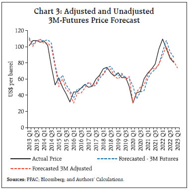
From the regression results, we find that the regression model is highly significant based on F statistic. Further, CA_US has a positive sign and is significant at 5 per cent level, while CA_CN has a negative sign and is highly significant at 1 per cent level.¹¹

The larger magnitude for the co-efficient for capacity utilisation for China implies that China is playing a more significant role in global crude oil dynamics. Any fall in the capacity utilisation for China would lead to the adjusted Brent 3-M futures forecast being revised downwards and vice-versa.

IV. Comparing Forecast Performance of Alternate Models

To evaluate the forecast performance of SPF crude oil forecast, the next quarter forecast for crude oil prices from the 7th to 27th round is taken as they are available with a quarterly frequency. From the 28th round, due to bi-monthly frequency, we proceed as follows. For Q2 and Q4 of each calendar year, an end of earlier period forecast is directly taken as they correspond to the quarter end. In the Q1 and Q3 of each calendar year, the forecast from the February round and August round is taken. It may be noted that this gives the forecaster some information advantage as they can incorporate information regarding crude oil price behaviour in the first 15-30 days of the forecasted quarter.

We first evaluate the forecast performance of unadjusted 3-month Brent futures prices (Chart 2). The unadjusted Brent 3M futures prices are seen to lag when used as a forecast measure, as they seem to be more influenced by the current spot prices than by futures price expectations.

First, we look at the average of forecast errors to see if there is a positive or negative bias in the forecast. In the period from Q2:2013 to Q1:2023, we find that the Brent 3M futures prices-based forecast has an average error of US$ 0.86, while for the SPF forecast, the average forecast error is US$ 1.56 and is US$ 0.72 for the PPAC no-change forecast and US$ 0.79 for Brent no-change forecast. It is however, the lowest for US-EIA forecast with an average forecast error of US$ (-)0.07.

The upward bias in the forecast may be due to various factors including the inability to predict sudden collapse in crude oil prices due to some unexpected demand collapse (as seen during COVID-19). It can also be due to the supply conditions normalising faster than expected or the temporary demand spike cooling off. Also, at times higher crude oil prices are due to collective actions of oil producers, namely OPEC, to restrain supply and drive-up oil prices but the supply cuts may not be successful for longer runs, with all producers having an incentive to increase their individual production to garner higher revenues, reflecting a classic game theory situation. Further, professional forecasters, forecasters at monetary authorities and even analysts using crude oil price forecast as an input may also tend to be conservative in the prediction for crude oil prices even when they expect the prices to cool down, reflecting loss aversion behaviour. This is because if the prices fail to cool down to the levels forecasted by them, a larger penalty is incurred in terms of higher inflation, thus raising questions over the efficacy of their forecasting prowess. On the other hand, if prices cool down more than expected it is a positive surprise in terms of cost and inflation, thereby escaping scrutiny. Thus, forecasters see lower perceived cost in forecasting a higher crude oil price and thus having an upward bias than predicting a lower crude oil price and risking scrutiny.

Next, we look at the forecast accuracy by evaluating the root mean square of error (RMSE). The Brent 3M futures prices show only a marginal improvement in the root mean square of error (RMSE) score over the Brent no-change forecast, highlighting the limitations of using unadjusted futures prices as a forecast. On the other hand, the SPF forecast significantly outperforms it in RMSE (Table 3). Further, the errors from futures prices are substantial during periods where there is a secular increase or decline in crude oil prices, as highlighted in the literature.

The comparison of the adjusted forecast vis-à-vis the unadjusted forecast shows that the adjusted forecast was able to better predict the fall in crude price during periods of a sudden drop in industrial activity like during the outbreak of COVID in 2020-21:Q1 and pickup in crude prices due to revival in industrial demand activity since 2020-21:Q2.

The improvement in prediction power of the adjusted Brent 3M futures prices forecast is reflected in its lower RMSE score of 6.89 down from 8.09 for the unadjusted forecast. This reflects a marked improvement over the no-change forecast. However, the SPF forecast continues to outperform, highlighting the advantage of using a combination of forecasts.

A snapshot view of the properties and merits and demerits of relying on all the above discussed sources of information are presented in Annex 1.

A critical factor in determining the predictive power of futures prices is the nature of the market in terms of whether the futures curve indicate a decline or an increase in prices going ahead. Therefore, in the next step, we identify the period of backwardation (the spot price of the asset is higher than the futures price) and contango (the spot price of the asset is lower than the futures price) and compare the forecast performance of various sources during these periods separately. Many plausible reasons for backwardation include short-term supply shortages, temporary demand spikes, expectations of deflation or recession, and convenience yield. Contango, conversely, usually occurs when the market predicts a supply shortage or demand spike in the future. Normal inflationary pressures and storage costs also lead to higher futures prices than the spot prices.

In the sample period considered, backwardation and contango are broadly equally occurring phenomenon. We find the average forecast error and RMSE separately for the period of backwardation and contango.¹² The forecast performance as measured by RMSE is less satisfactory when the market prices are in contango, with a large positive upward bias in the forecast being found as measured by the average of forecast error. This implies that when the futures oil prices are trading higher; all the forecast models overpredict oil prices, thus leading to a substantial upward error in forecast.

The magnitude of error in a scenario of contango is the highest in the case of Brent’s 3-month futures price-based unadjusted forecast. This bias in prediction is also reflected in a higher RMSE of 9.19 during the period of contango as contrasted with an RMSE of 7.00 during the backwardation period. The adjusted Brent 3-month futures considerably reduces this bias during the contango periods, resulting in RMSE improving to 7.88 from 9.19. This improvement can be attributed to the inclusion of the forward-looking economic indicators of oil demand, which helps to predict any demand shock-induced collapse in oil prices. Similarly, under backwardation, Brent 3-month adjusted futures perform almost as well as the SPF forecast.

IV. Conclusion

In this article, we looked at the relative performance of various forward-looking sources of information of oil prices in terms of their forecast accuracy. We find that qualitative information such as the median forecast available from the SPF tends to outperform futures prices; and futures prices, at best, can match a naïve forecast where we assume that the prices would continue to remain the same at the current level. We, however, find that the predictive power of futures prices improves significantly once we account for the impact of industrial activity on oil demand by incorporating information on capacity utilisation for the two largest consumers of crude oil, the US and China. Our results also indicate that the forecast performance of all the sources analysed is better under a backwardation period, when current prices are higher than futures prices. These indicate that relying upon any specific individual source of information alone may not be the prudent approach and an assessment of the future trajectory of oil prices should ideally take into account all the available information from various data sources, trends in actual economic activity in major oil consuming economies. Moreover, the current state of the oil market as indicated by the shape of futures curve, i.e., whether it is in contango or backwardation, also provides valuable information regarding the degree of accuracy with which crude oil prices can be forecasted.

References

Abosedra, S., & Baghestani, H. (2004). On the predictive accuracy of crude oil futures prices. Energy Policy, 32(12), 1389–1393. https://doi.org/10.1016/S0301-4215(03)00104-6

Ahmad, I., Iqbal, S., Khan, S., Han, H., Vega-Muñoz, A., & Ariza-Montes, A. (2022). Macroeconomic effects of crude oil shocks: Evidence from South Asian countries. Frontiers in Psychology, 13(August). https://doi.org/10.3389/fpsyg.2022.967643

Alquist, R., Kilian, L., & Vigfusson, R. J. (2011). Forecasting the Price of Oil. In International Finance Discussion Papers (Issue 1022).

Bashiri Behmiri, N., & Pires Manso, J. R. (2013). Crude Oil Price Forecasting Techniques: A Comprehensive Review of Literature. SSRN Electronic Journal, 1–32. https://doi.org/10.2139/ssrn.2275428

Baumeister, C., & Kilian, L. (2012). Real-time forecasts of the real price of oil. Journal of Business and Economic Statistics, 30(2), 326–336. https://doi.org/10.1080/07350015.2011.648859

Baumeister, C., & Kilian, L. (2014a). Real-time analysis of oil price risks using forecast scenarios. IMF Economic Review, 62(1), 119–145. https://doi.org/10.1057/imfer.2014.1

Baumeister, C., & Kilian, L. (2014b). What central bankers need to know about forecasting oil prices. International Economic Review, 55(3), 869–889. https://doi.org/10.1111/iere.12074

Baumeister, C., & Kilian, L. (2015). Forecasting the Real Price of Oil in a Changing World: A Forecast Combination Approach. Journal of Business and Economic Statistics, 33(3), 338–351. https://doi.org/10.1080/07350015.2014.949342

Blanchard, O. J., & Gali, J. (2007). The Macroeconomic Effects of Oil Shocks: Why are the 2000s So Different from the 1970s? National Bureau of Economic Research No. 15467, Cambridge, USA.

Bredin, D., O’Sullivan, C., & Spencer, S. (2021). Forecasting WTI crude oil futures returns: Does the term structure help? Energy Economics, 100(April), 105350. https://doi.org/10.1016/j.eneco.2021.105350

Chinn, M., LeBlanc, M., Coibion, O., Chinn, M., LeBlanc, M., & Coibion, O. (2005). The Predictive Content of Energy Futures: An Update on Petroleum, Natural Gas, Heating Oil and Gasoline.

Chu, P. K., Hoff, K., Molnár, P., & Olsvik, M. (2022). Crude oil: Does the futures price predict the spot price? Research in International Business and Finance, 60(August 2021). https://doi.org/10.1016/j.ribaf.2021.101611

da Silva Souza, R., & de Mattos, L. B. (2023). Macroeconomic effects of oil price shocks on an emerging market economy. Economic Change and Restructuring, 56(2), 803–824. https://doi.org/10.1007/s10644-022-09445-w

ECB. (2015). Forecasting the price of oil (Issue 4).

Frey, G., Manera, M., Markandya, A., & Scarpa, E. (2009). Econometric models for oil price forecasting: A critical survey. CESifo Forum, 10(1), 29–44.

Funk, C. (2018). Forecasting the real price of oil - Time-variation and forecast combination. Energy Economics, 76, 288–302. https://doi.org/10.1016/j.eneco.2018.04.016

Garga, V., Lakdawala, A., & Sengupta, R. (2022). Assessing Central Bank Commitment to Inflation Targeting: Evidence From Financial Market Expectations in India. SSRN Electronic Journal, 22. https://doi.org/10.2139/ssrn.4245158

Gulen, G. (1998). Efficiency in the crude oil futures market. Journal of Energy Finance & Development, 3(1), 13–21.

John, J., Singh, S., & Kapur, M. (2020). Inflation Forecast Combinations – The Indian Experience. RBI Working Paper Series, September.

Kilian, L. (2009). Not all oil price shocks are alike: Disentangling demand and supply shocks in the crude oil market. American Economic Review, 99(3), 1053–1069. https://doi.org/10.1257/aer.99.3.1053

Manescu, C., & Robays, I. Van. (2014). FORECASTING THE BRENT OIL PRICE ADDRESSING TIME-VARIATION IN FORECAST PERFORMANCE (1735).

Merino, A., & Alvaro Ortiz. (2005). Explaining the so-called price premium in oil markets.

Pagano, P., & Pisani, M. (2009). Risk-adjusted forecasts of oil prices (999).

Sadath, A., & Acharya, R. (2021). The macroeconomic effects of increase and decrease in oil prices: evidences of asymmetric effects from India. International Journal of Energy Sector Management, ahead-of-p. https://doi.org/10.1108/IJESM-02-2020-0009

Wang, Y., Liu, L., Diao, X., & Wu, C. (2015). Forecasting the real prices of crude oil under economic and statistical constraints. Energy Economics, 51, 599–608. https://doi.org/10.1016/j.eneco.2015.09.003

Yang, C. W., Hwang, M. J., & Huang, B. N. (2002). An analysis of factors affecting price volatility of the US oil market. Energy Economics, 24(2), 107–119. https://doi.org/10.1016/S0140-9883(01)00092-5

Ye, M., Zyren, J., & Shore, J. (2002). Forecasting crude oil spot price using OECD petroleum inventory levels.

International Advances in Economic Research, 8(4), 324–333. https://doi.org/10.1007/BF02295507

Ye, M., Zyren, J., & Shore, J. (2005). A monthly crude oil spot price forecasting model using relative inventories. International Journal of Forecasting, 21(3), 491–501. https://doi.org/10.1016/j.ijforecast.2005.01.001

Zhang, Y., Ma, F., Shi, B., & Huang, D. (2018). Forecasting the prices of crude oil: An iterated combination approach. Energy Economics, 70, 472–483. https://doi.org/10.1016/j.eneco.2018.01.027

^{^} The authors are from the Department of Economic and Policy Research. The views expressed in this article are those of the authors and not of the Reserve Bank of India.

¹ In naïve forecasting, it is assumed that the price of crude oil at time t+1 is equal to the same at time t (current price). In other words, it is a no-change forecast.

² Futures (plural) is being used to refer to futures contract based price, while future (singular) is used to refer to future as tense.

³ These encompass methodologies like the Delphi method, belief networks, fuzzy logic, expert systems, and web text mining.

⁴ These forecasters also use econometric as well as structural models as inputs for making their assessments, but do not solely rely on them.

⁵ The composition of Indian Basket of Crude represents Average of Oman & Dubai for sour grades and Brent (Dated) for sweet grade in the ratio of crude processed during previous financial year. The data for Indian Basket of Crude is provided by the Petroleum Planning & Analysis Cell (PPAC) under the Ministry of Petroleum and Natural Gas for both daily and monthly frequencies.

⁶ Our assumption is that the trajectory of brent futures could adequately capture the same of Indian basket within the forecast relevant period (one quarter).

⁷ The average of daily price of Brent 3 month ahead futures in the preceding quarter is taken as the forecast for the next quarter.

⁸ Unadjusted futures prices based forecast.

⁹ We use one period lag for capacity utilisation as the data on capacity utilisation is available with a lag of one quarter. So, for a forecaster at time t, only information about CU of t-1 is available. Given that CU has a high level of persistence, previous period CU is taken as a proxy.

¹⁰ Augmented Dickie Fuller (ADF) showed that the series are stationary (Forecast error and capacity utilisation of China at 1 per cent significance and for capacity utilisation for US at 10 per cent significance).

¹¹ The CU for US shows up in the regression with an opposite sign than expected which could be also indicative of the fact that futures prices, are putting more weight on US CU whereas it is underweighting China CU (which is reflected in the negative sign).

¹² Backwardation and Contango are estimated in the quarter the forecasts are made.