by Harshita Keshan, Garima Wahi and Krishna Mohan Kushwaha^{^}

The article presents an analysis of the fiscal-inflation nexus, and insights into the evolving dynamics of global public debt in the post-pandemic era. The pandemic triggered unprecedented fiscal expansions and accommodative monetary policies, contributing to a surge in global debt levels and multi-decadal high inflation. Employing a panel vector autoregression (PVAR) framework, the study finds that inflationary surprises can only temporarily reduce real debt burdens while large deficits amplify inflationary pressures.

Introduction

The COVID-19 pandemic, a true black swan event, triggered an unprecedented fiscal and monetary stimulus across the world to support domestic demand and preserve financial stability. Even as such coordinated policy responses prevented market frenzy and supported quick economic recoveries, these responses led to inflated central bank balance sheets and surging public debt levels, contributing to multi-decadal high inflation amidst lingering supply bottlenecks. While the vast quantitative easing (QE) during 2010s after the global financial crisis did not provoke inflation, the unparalleled fiscal stimulus during the pandemic in conjunction with extremely accommodative monetary policies sent inflation soaring globally, raising the question whether inflation is a fiscal phenomenon (The Economist, 2021).

As countries modified fiscal targets and activated escape clauses, global public debt surged from 84 per cent of gross domestic product (GDP) in 2019 to near 100 per cent of GDP in 2020. Subsequently, as exceptional fiscal measures came to an end, fiscal deficits corrected in some cases (but still elevated) and nominal GDP posted robust growth, global debt decreased to around 91 per cent of GDP by end-2022. It increased thereafter to around 93 per cent in 2024 and is poised to increase further from burgeoning interest burdens and the slow pace of fiscal consolidation, casting aspersions on debt sustainability (IMF, 2024a).

The multi-decadal high inflation during 2022- 2023 and high nominal GDP growth appear to have contributed to eroding the real value of government debt in the post-pandemic period. This well-documented debt-reduction mechanism is effective only when inflation surpasses expectations, as positive inflation surprises boost nominal GDP and tax revenues (Patel and Peralta-Alva, 2024; Garcia-Macia 2023); however, this channel could be transient and unsustainable as repeated inflation surprises can destabilise inflation expectations, depress economic activity, drag down government revenues and exacerbate fiscal deficits and public debt. At the same time, prudent fiscal policy also supports monetary policy in anchoring inflation expectations. Sargent and Wallace (1981) seminal paper illustrates that sustained large government fiscal deficits, even if not financed by central banks, can undermine the effectiveness of monetary policy in curbing inflation.

These intricate fiscal-financial interactions create a dual and dynamic relationship between inflation and debt. While studies which explore inflation and government debt dynamics focus on one side of the relationship at a time, this article tries to evaluate the fiscal-inflation nexus in a comprehensive framework of panel vector autoregression (PVAR). Before delving into the econometric analysis, it is essential to first examine the emerging trends in global public debt as outlined in the next section. It provides crucial context, offering insights into the distributional dynamics of debt and its evolution, shaped significantly by the pandemic and subsequent policy responses. Section III summarises the nature of work done in this field and the results of these studies. Section IV provides an in-depth discussion of the model employed, the rationale underpinning its selection, and the detailed steps involved in its implementation. Section V presents the results and inferences therefrom with the last section providing concluding remarks.

II. Stylised Facts

The pandemic-induced policy response has profoundly influenced global public debt. According to the IMF Fiscal Monitor (October 2024), global public debt is anticipated to surpass $100 trillion in 2024 – equivalent to 93 per cent of global GDP – and is projected to approach 100 per cent of GDP by 2030. This trajectory underscores the significant fiscal challenges that lie ahead.

Chart 1a vividly depicts the rising trend of global public debt, highlighting its alarming growth trajectory in dollar value terms for the world as a whole and some countries which have particularly large value of debt. Notably, while worsening debt burdens are projected for only one-third of the world’s economies, this subset contributes to more than half of total global debt and approximately two-thirds of global GDP, emphasising the concentrated nature of fiscal vulnerabilities (IMF, 2024b).

Further insights into the distribution of debt burdens are provided in Chart 1b where debt is examined relative to GDP. The persistently higher mean compared to the median debt-to-GDP signals a positively skewed distribution, indicating that a few highly indebted economies significantly inflate the average. Over time, the divergence between median and mean ratios has widened, signifying an increasingly skewed debt distribution. An analysis of advanced economies (AEs) and emerging markets and middle-income economies (EMMEs) indicates that the average debt-to-GDP ratio for AEs is nearly 40 percentage points higher than that for EMMEs. Despite a modest increase in global debt-to-GDP ratio, AEs led by the US are expected to maintain their dominant share of global debt, even as the debt levels of EMMEs steadily rise driven by China.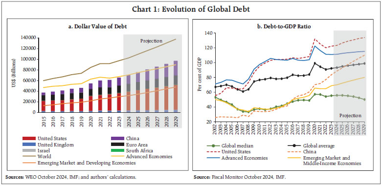

As pandemic-related restrictions eased and economies began to rebound in 2022, resilient growth and inflationary surprises provided a temporary reprieve for fiscal balances. Chart 2 illustrates how primary deficits returned to pre-pandemic lows by 2022, especially for AEs — reducing by approximately eight percentage points for AEs and four percentage points for EMMEs compared to their 2020 levels. The progress, however, remains wobbly on the overall deficit front owing to rising interest payments. Overall fiscal deficits are expected to increase marginally till 2024 to 5.2 per cent of GDP, driven by higher interest expenses and continued public spending, before gradually declining during the period 2025–2029. Nevertheless, fiscal deficits are expected to remain above pre-pandemic levels for most countries over the coming years.

In 2022, when inflation spiked, several countries experienced revenue surprises from increased tax buoyancy, and concomitantly, surging nominal GDP levels drove down deficit and debt ratios. On average, AEs witnessed a jump of around 3 per cent in government revenues between 2020 and 2022 while EMMEs revenues increased by around 5 per cent over the same time period (Chart 3). However, for EMMEs with significant foreign currency-denominated debt, fiscal dynamics deteriorated due to currency depreciation and rising interest rates.

The trajectory of inflation steadily increased starting 2020 while debt-to-GDP ratio witnessed a concomitant reduction from its peak, reaching its trough in tandem with the inflation peak in 2022, highlighting a negative correlation between positive inflation surprises and debt-to-GDP ratios (Chart 4). However, such high inflation-led debt deflation may offer only short-term relief and sustained fiscal consolidation efforts are required for effective debt consolidation. The next section summarises the nature of work done in this field and the results of these studies.

III. Literature Review

An increase in inflation affects the fiscal outlook through various channels (Dynan, 2022). First, higher inflation raises interest cost for the government due to rolling over of debt at higher interest rates. Second, inflation impacts primary balance both positively and negatively. It instantly increases the nominal revenue, especially the ones not indexed to inflation, like taxes above income thresholds; but also raises the spending due to increased expenditure on inflation-indexed benefit programs. Third, inflation also brings about a higher nominal GDP growth, helping the government to bear the burden of higher nominal government debt on the one hand and reducing debt-to-GDP ratio through the denominator channel on the other. This effect is significant and may overshadow the first and second ones.

The impact of inflation surprises on debt and fiscal balances is also established empirically. Garcia-Macia (2023) finds that as nominal revenues are affected by inflation immediately while primary expenditures take time to adjust, inflation shocks temporarily improve fiscal balances. Inflationary shocks, and not merely inflation, also improve debt dynamics by improving the primary balance and the nominal GDP as denominator. Unexpected inflation has played a significant role in driving the debt-to-GDP ratio during certain periods and in specific countries. GDP shocks have also been influential, accounting for an estimated 40 per cent of the yearly variation in debt-to-GDP ratios for the median advanced economy (Patel and Peralta-Alva, 2024). However, if inflation is caused due to a supply shock, for example, higher energy prices, it can also adversely affect the public finances by moderating consumption and reducing tax revenues (Bankowski et al., 2023).

In the US, debt-to-GDP ratio is determined by contributions from inflation, growth and nominal returns paid on debts of different maturities (Hall and Sargent, 2011). Das and Ghate (2022) find a higher contribution from inflation and growth towards reduction in debt-to-GDP for India during high inflationary and growth years. Several other studies use inflation, GDP growth, and interest rates as drivers of debt to evaluate the evolution of debt-to-GDP ratio (Ando et al., 2025).

On the other side, literature also highlights the potential link between expansionary fiscal policy and inflation. The fiscal theory of the price level (Cochrane, 2021) postulates that when real value of government debt is more than the present value of taxes less spending, it can drive up prices to restore solvency of public finances. Although some studies establish that public debt is inflationary for countries with large public debt (Kwon, 2009; Romero and Marin, 2017), others find that debt only plays a minor role in the determination of price level (Castro et al., 2003; Harmon, 2012). A few studies also explore the prospect of non-linear impact on inflation, wherein the inflation response varies with the level of debt. (Cevik and Miryugin, 2024; Beirne and Renzhi, 2024). Banerjee et al. (2023) also establish that fiscal deficit has a non-linear impact on inflation – greater impact on upside tail risks than on average inflation – and that these effects are significantly larger for Emerging Market and Developing Economies (EMDEs) as compared to AEs. They also find that in inflation targeting regimes, the effect of higher fiscal deficit on inflation weakens sharply. Martin (2015) infers that higher public debt leads to increased inflation in the longer run unless the country imposes a strict inflation target. On the expectations front, evidence indicates that debt surprises can raise long-term inflation expectations in Emerging Market Economies (EMEs) persistently, especially when initial debt and inflation levels are high (Brandao-Marques et al., 2024).

In AEs, higher deficits under fiscal-led regime have five times larger effect on inflation vis-à-vis monetary-led regime, in addition to raising the likelihood of high inflation (Banerjee et al., 2022). Leeper (1991) demonstrated that active fiscal behaviour leads to lump-sum inflation tax, generating inflation in the next period while Bordo and Levy (2021) find that the association between fiscal deficits and inflation holds during periods of fiscal stress when governments resort to inflation tax. The degree of impact of fiscal deficits on inflation can also depend on prevailing inflationary conditions (Lin and Chu, 2013).

Catao and Terrones (2005), in their study of 107 nations, identify a significant positive relationship between fiscal deficits and inflation in economies experiencing high inflation and in developing countries, however, they also find that this relationship does not hold for low-inflation, advanced economies. Some studies also attempt to assess the bidirectional relationship between fiscal variables and inflation, but by establishing one causality at a time. In Euro area, inflation affects public finances negatively beyond short run while fiscal expansion exacerbates inflationary pressures, necessitating a stronger monetary policy response (Bankowski et al., 2023). According to Bon (2015), in developing countries, public debt seems to increase inflation, while inflation reduces public debt. In another study of nine EU countries, Tiwari et al. (2015) establish a causality from inflation to budget deficits for Belgium and France but find no causality from budget deficits to inflation.

A few studies testing the two-way causality between public debt and inflation in a unified framework (using either VAR or VECM) have typically focused on a single country like the US (Cherif and Hasanov, 2018) and Germany (Nastansky et al., 2014). Overall, the relationship between fiscal deficits and inflation has primarily been explored from one perspective, and often in the context of one country or few large economies. This paper builds upon these studies to investigate two-way relationship between inflation and public debt, across a diverse set of forty-two countries, including both advanced and emerging economies.

IV. Data and Methodology

In order to examine the interplay of fiscal dynamics (debt-to-GDP ratio) with other macroeconomic indicators, including economic growth, inflation, and policy rates, this study employs a Panel Vector Autoregression (PVAR) framework. The PVAR approach effectively accounts for country-specific heterogeneity while capturing the dynamic interdependencies among multiple endogenous variables. Although VAR models are well-suited for estimating such relationships, their empirical application in macroeconomic studies often encounter challenges related to limited data availability, commonly referred to as the “curse of dimensionality”.

In this study, relatively short time series further limits the feasibility of estimating separate VAR models for individual countries. To address this constraint, the analysis focuses on a concise set of variables that represent the core dynamics of key macroeconomic indicators and adopts a panel VAR framework. This pooling of data across countries not only mitigates the limitations of short time series but also enhances estimation reliability by leveraging the cross-sectional dimension of the dataset (Adarov, 2021). The specification takes the following reduced form:

with time index t = 1,…,T; and country index i = 1,…, N, where y_i is a vector of five variables for country i: real GDP growth rate, CPI inflation rate (year-on-year), Δ debt-to-GDP ratio, policy rate and oil price inflation; γ_i is a vector of country specific fixed effects; and ε_i,t denotes a vector of reduced form errors.

To account for the substantial cross-sectional heterogeneity, the model incorporates country fixed effects (γ_i) to capture the unobserved, time-invariant characteristics unique to each nation. However, since fixed effects may correlate with the regressors due to the lagged dependent variables, we address this potential bias using forward mean-differencing, commonly known as the ‘Helmert procedure’, as outlined by Love and Zicchino (2006). This approach retains the orthogonality between the transformed variables and lagged regressors, allowing lagged regressors to serve as valid instruments for estimating coefficients using the system GMM method. We employ robust standard errors to account for potential heteroskedasticity and serial correlation within the data.

Since the model is estimated in its reduced form, additional structure is imposed on the error variance-covariance matrix to identify structural shocks using a standard Cholesky decomposition, which orthogonalises the reduced-form errors. In this framework, variables listed earlier in the ordering are treated as more exogenous, influencing subsequent variables both contemporaneously and with a lag. The chosen ordering for the Cholesky decomposition is: oil inflation→ CPI inflation→ GDP growth → debt-to-GDP ratio → policy rate. The primary findings remain robust to different permutations of ordering.

IV.1. Data

This econometric analysis utilises an unbalanced panel dataset comprising a global sample of forty-two countries, including 15 AEs and 27 EMEs, spanning the period 1990–2023 at an annual frequency. The composition of the sample is detailed in Appendix Table A1. The selection of countries is primarily driven by the availability of sufficiently long time series and a substantial number of cross-sectional observations (N), ensuring the feasibility of a robust econometric analysis. The macroeconomic variable datasets, namely GDP, CPI, and debt-to-GDP ratio, are sourced from the IMF’s World Economic Outlook Database (October 2024). Oil price data are obtained from the World Bank’s Pink Sheet, while policy rate data are retrieved from CEIC. Table 1 presents the descriptive statistics for all variables¹.

V. Empirical Results

We begin by assessing the stationarity of the variables used in Section V.1 and determine the optimal lag length for our model based on the Moment and Model Selection Criteria (MMSC) in Section V.2. Then we test for Granger causality between the primary variables and present the impulse response functions, analysing the response of the key variables to various shocks, providing graphical representations alongside detailed explanations of the observed effects (Sections V.3 and V.4).

V.1. Test for Stationarity

All variables are retained in their original form, except for the debt-to-GDP ratio, which is used in first differences. Stationarity is verified using the Im-Pesaran-Shin, Fisher Augmented Dickey-Fuller, and Fisher Phillips-Perron panel unit root tests, with the results presented in Table 2.

V.2. Model Selection

The selection of the appropriate lag order is critical for a robust panel VAR analysis. Selecting too few lags can omit critical variables, biasing results, while excessive lags risk over-parameterization and reduced degrees of freedom (Boubtane et al., 2012). We use one lag based on the MMSC (Andrews and Lu, 2001), specifically the Modified Bayesian Information Criterion (MBIC) and the Modified Hannan-Quinn Information Criterion (MQIC). The overall coefficient of determination (CD) also supports this choice. The combined results reported in Table 3 validate the selection of a first order PVAR² model, ensuring a balance between explanatory power and parsimony.³

V.3. Granger Causality

Before proceeding further, we examine Granger causality between key variables, particularly the CPI and debt-to-GDP ratio. Table 4 reports the chi-square Wald statistics for testing the null hypothesis that the debt-to-GDP ratio does not Granger cause CPI and vice versa, as well as its causal effects on the other three variables. The last row presents the joint probability for all lagged variables in the equation, evaluating whether all lags of all variables can be excluded from each equation in the panel VAR system. The findings indicate bidirectional causality between the debt-to-GDP ratio and CPI at 1 per cent significance level. Furthermore, the joint significance chi-square statistics in the final row confirm that all lagged variables collectively Granger cause each variable in the system.

V.4. Impulse Response Functions

We now proceed with the analysis of the impulse response functions (IRFs) to assess the responses of the debt-to-GDP ratio and CPI to shocks in the corresponding variables within the system. Chart 5 presents IRF plots for debt-to-GDP ratio and CPI. The solid lines in the plots represent the orthogonal IRFs of the respective variables over a ten-year horizon. The shaded areas indicate 95 per cent confidence intervals constructed using 1,000 Monte Carlo simulations based on the fitted reduced form of the panel VAR model.

As shown in Chart 5, a positive shock to the debt-to-GDP ratio has a positive and significant short-term impact on CPI inflation, which diminishes over time. Specifically, the estimates indicate that a one standard deviation shock to debt-to-GDP ratio (3.7 percentage points) can lead to a 120 basis points (bps) rise in CPI inflation in the first period, peaking at 181 bps in the second period. This effect remains significantly positive up to 5 years.

Analysing the other side of the bidirectional relationship, Chart 5 illustrates that higher inflation causes a significant and sharp fall in debt-to-GDP ratio. Specifically, a one standard deviation shock to inflation (4.4 percentage points) can lead to around 38 bps reduction in debt-to-GDP ratio in first year. The impact peaks in the third year and fades by the seventh year, supporting the evidence provided by Garcia-Macia (2023).

Beyond the primary variables of interest, the interactions among other variables also appear to be on expected lines (Appendix Chart A1). For instance, an increase in the policy rate significantly reduces inflation, demonstrating the effectiveness of monetary policy.

VI. Conclusion

This study analyses the intricate relationship between inflation and public debt, particularly in the context of unprecedented fiscal spending triggered by the COVID-19 pandemic. The findings underscore the inflationary effects of high public debt, emphasising the necessity of fiscal consolidation. While high inflation can temporarily deflate away debt burden, this effect is neither permanent nor sufficient to address long-term fiscal challenges. High inflation can have its own adverse consequences on consumption, investment, and growth (RBI, 2024).

References

Adarov, A. (2021). Dynamic interactions between financial cycles, business cycles and macroeconomic imbalances: A panel VAR analysis. International Review of Economics & Finance, 74, 434-451.

Ando, S., Mishra, P., Patel, N., Peralta-Alva, A., & Presbitero, A. F. (2025). Fiscal consolidation and public debt. Journal of Economic Dynamics and Control, 170, 104998.

Banerjee, R., Boctor, V., Mehrotra, A. N., & Zampolli, F. (2023). Fiscal sources of inflation risk in EMDEs: The role of the external channel. Bank for International Settlements, Monetary and Economic Department.

_______(2022). Fiscal deficits and inflation risks: The role of fiscal and monetary regimes. Bank for International Settlements, Monetary and Economic Department.

Bańkowski, K., Checherita-Westphal, C., Jesionek, J., & Muggenthaler, P. (2023). The effects of high inflation on public finances in the euro area: Based on the analysis by the Eurosystem members of the Working Group on Public Finance. ECB Occasional Paper No. 332.

Beirne, J., & Renzhi, N. (2024). Debt shocks and the dynamics of output and inflation in emerging economies. Journal of International Money and Finance, 148, 103167.

Bordo, M. D., & Levy, M. D. (2021). Do enlarged fiscal deficits cause inflation? The historical record. Economic Affairs, 41(1), 59-83.

Bon, N. V. , (2015). The Relationship Between Public Debt and Inflation in Developing Countries: Empirical Evidence Based on Difference Panel GMM. Asian Journal of Empirical Research, 5(9), 128–142.

Boubtane, E., Coulibaly, D., & Rault, C. (2013). Immigration, growth, and unemployment: Panel VAR evidence from OECD countries. Labour, 27(4), 399-420.

Brandao-Marques, L., Casiraghi, M., Gelos, G., Harrison, O., & Kamber, G. (2024). Is high debt constraining monetary policy? Evidence from inflation expectations. Journal of International Money and Finance, 149, 103206.

Castro, R., de Resende, C., & Ruge-Murcia, F. (2003). The backing of government debt and the price level. Cahier de recherche, 22.

Catao, L. A., & Terrones, M. E. (2005). Fiscal deficits and inflation. Journal of Monetary Economics, 52(3), 529-554.

Cevik, S., & Miryugin, F. (2024). It’s never different: Fiscal policy shocks and inflation. Comparative Economic Studies, 1-35.

Cherif, R., & Hasanov, F. (2018). Public debt dynamics: the effects of austerity, inflation, and growth shocks. Empirical Economics, 54, 1087-1105.

Cochrane, J. H. (2021). The fiscal theory of the price level: An introduction and overview. Journal of Economic Perspectives.

Das, P., & Ghate, C. (2022). Debt decomposition and the role of inflation: A security level analysis for India. Economic Modelling, 113, 105855.

Dynan, K. (2022, September). High inflation and fiscal policy. Peter G. Peterson Foundation.

Garcia-Macia, D. (2023). The effects of inflation on public finances. IMF Working Paper No. 93.

Hall, G. J., & Sargent, T. J. (2011). Interest rate risk and other determinants of post-WWII US government debt/GDP dynamics. American Economic Journal: Macroeconomics, 3(3), 192-214.

Harmon, E. Y. (2012). The impact of public debt on inflation, GDP growth and Interest rates in Kenya (Doctoral dissertation, University of Nairobi).

Has the pandemic shown inflation to be a fiscal phenomenon? A decade of QE did not cause much inflation. Fiscal stimulus has sent it soaring. (2021). In The Economist. Retrieved from https://www.economist.com/finance-and-economics/2021/12/18/has-the-pandemic-shown-inflation-to-be-a-fiscal-phenomenon.

International Monetary Fund (2024a). Fiscal Affairs Dept. Fiscal Monitor, October 2024: Putting a Lid on Public Debt.

_______(2024b). World Economic Outlook, October 2024: Policy Pivot, Rising Threats.

Kwon, G., McFarlane, L., & Robinson, W. (2009). Public debt, money supply, and inflation: a cross-country study. IMF Staff Papers, 56(3), 476-515.

Lin, H. Y., & Chu, H. P. (2013). Are fiscal deficits inflationary? Journal of International Money and Finance, 32, 214-233.

Love, I., & Zicchino, L. (2006). Financial development and dynamic investment behavior: Evidence from panel VAR. The Quarterly Review of Economics and Finance, 46(2), 190-210.

Martin, F. M. (2015). Debt, inflation and central bank independence. European Economic Review, 79, 129-150.

Leeper, E. M. (1991). Equilibria under ‘active’ and ‘passive’ monetary and fiscal policies. Journal of Monetary Economics, 27(1), 129-147.

Nastansky, A., Mehnert, A., & Strohe, H. G. (2014). A vector error correction model for the relationship between public debt and inflation in Germany. University Of Potsdam, Statistical Discussion Contributions No. 51.

Patel, N., & Peralta-Alva, A. (2024). Public Debt Dynamics and the Impact of Fiscal Policy. IMF Working Paper No. 87.

Reserve Bank of India (2024, December 6). Statement by the Governor, Shri Shaktikanta Das: Monetary Policy Statement for December 2024.

Romero, J. P. B., & Marín, K. L. (2017). Inflation and public debt. Monetaria, 5(1), 39-94.

Sargent, T. J., & Wallace, N. (1981). Some unpleasant monetarist arithmetic. Federal Reserve Bank Of Minneapolis Quarterly Review, 5(3), 1-17.

Tiwari, A. K., Bolat, S., & Koçbulut, Ö. (2015). Revisit the budget deficits and inflation: Evidence from time and frequency domain analyses. Theoretical Economics Letters, 5(03), 357.

Appendix

^{^} The authors are from the Monetary Policy Department, Reserve Bank of India (RBI). Assistance with data processing from Akash Raghatwan is gratefully acknowledged. The views expressed in this article are those of the authors and do not represent the views of the RBI.

¹ The data has been winsorised at 97 per cent, meaning the top and bottom 1.5 per cent of values are adjusted.

² To ensure the GMM model is overidentified, four lags are used as instruments. Overidentification allows the application of various MMSC criteria, which are not applicable in just-identified models.

³ The selected model passes the stability test.