The Indian banking sector embarked upon a phase of consolidation during H2:2021-22. Banks bolstered risk absorbing capacity as gross non-performing assets declined to their lowest level in six years. Macro stress tests reveal that all banks would be able to comply with minimum capital adequacy norms even in a severe stress scenario, although some segments as well as non-banking financial companies may be vulnerable to liquidity shocks. Contagion risks increased in March 2022 vis-à-vis September 2021 on account of deepening inter-bank market linkages. Introduction 2.1 Policy support, including regulatory dispensations, helped the Indian banking sector navigate waves of the pandemic and strengthen their risk absorption capacity. With the progressive normalisation of economic activity, banks were able to kick start a fresh lending cycle while simultaneously improving profitability. There are, however, early signs of stress in certain sectors, calling for caution and monitoring on an ongoing basis. 2.2 This chapter presents an evaluation of the soundness and resilience of financial intermediaries in India by analysing their recent performance on key parameters, as reflected in their offsite reporting to the Reserve Bank. Section II.1 presents an assessment of business mix, asset quality, capital adequacy, earnings and profitability of scheduled commercial banks (SCBs) and evaluates their resilience against macroeconomic shocks through stress tests and sensitivity analysis. Section II.2 provides a snapshot of the performance of small finance banks (SFBs). Sections II.3 and II.4 examine the recent financial performance of urban cooperative banks (UCBs) and non-banking financial companies (NBFCs) and stress tests their resilience. The concluding Section II.5 provides a detailed analysis of the network structure and connectivity of the Indian financial system and presents the results of contagion analysis under adverse scenarios. II.1 Scheduled Commercial Banks (SCBs)1, 2 2.3 After reaching a high of 11.9 per cent in March 2021, aggregate deposit growth (y-o-y) moderated gradually through 2021-22 reaching 9.9 per cent in March 2022 and further to 9.1 per cent by June 3, 2022 (Chart 2.1 a). Growth in current and savings account (CASA) deposits also moderated during this period, primarily on account of public sector banks (PSBs). Nevertheless, CASA deposit growth has exceeded the growth of term deposits for all categories of banks during the COVID-19 pandemic, which partly reflects households’ preference for liquidity in the face of higher uncertainty (Chart 2.1 b). 2.4 As the recovery gained traction, bank credit picked up during H2:2021-22 and reached 11.5 per cent in March 2022, rising further to 12.9 per cent as on June 3, 2022. Lending by both PSBs and private sector banks (PVBs) increased (Chart 2.1 c). While credit growth in the agriculture sector declined marginally despite a step-up in lending by PVBs, industrial credit continued to strengthen, driven by robust lending by PVBs and Foreign Banks (FBs). PSBs too recorded growth in industrial credit after almost three years of contraction (Chart 2.1 e). Lending to the services sector accounted for 41.8 per cent of credit extended by FBs (Chart 2.1 d). Growth in personal loans3 remained steady during 2021-22 and accounted for over 30 per cent of incremental lending by PSBs and PVBs. In personal loan sector, housing loans, credit card receivables and vehicle/ auto loans recorded double digit growth (Chart 2.1 f). 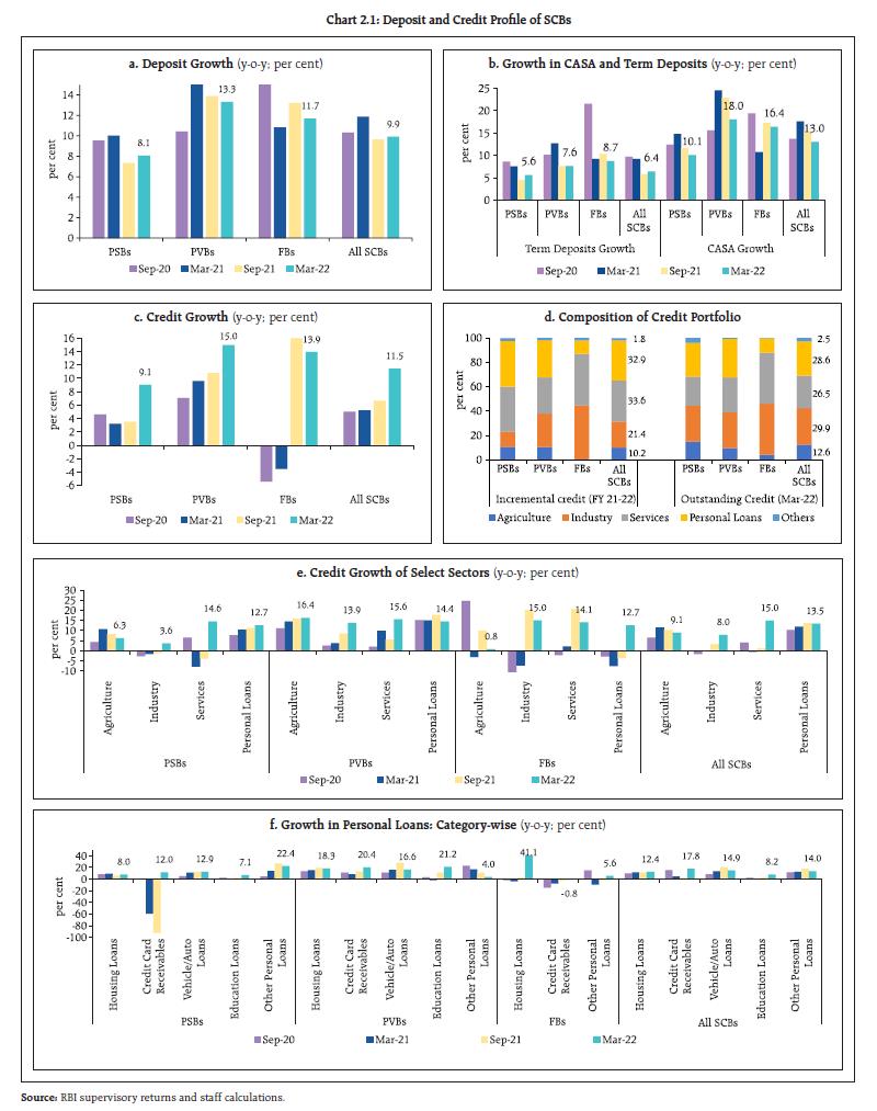
| Table 2.1: Increase in New Loans by SCBs: Economic Sectors and Organisations* | | Sector | Q4:2020-21 | Q1:2021-22 | Q2:2021-22 | Q3:2021-22 | Q4:2021-22 | | Increase during the quarter (₹ ‘000 crore) | | Economic Sector wise | | Agriculture | 13 | -50 | 72 | 3 | 24 | | Industry | 57 | -134 | 63 | 110 | 36 | | Services | 121 | -226 | 116 | 100 | 116 | | Personal Loans | 31 | -135 | 114 | 41 | 55 | | Organisation wise | | Public Sector | 64 | -133 | 49 | 101 | 57 | | Private Corporate Sector | 99 | -146 | 73 | 74 | 97 | | Household Sector | 64 | -285 | 268 | 76 | 85 | | of which: Individuals | 47 | -235 | 227 | 58 | 66 | | Others | -3 | 2 | 3 | 10 | 1 | | Total | 223 | -562 | 393 | 261 | 239 | | Share of new loans in total loans (per cent) | 16.7 | 11.6 | 15.1 | 16.8 | 17.9 | Note: *excluding Regional Rural Banks (RRBs).
Source: Basic Statistical Returns - 1, RBI. | 2.5 Rapid credit expansion during the second half of 2021-22 was aided by new loan accounts in the industrial and services sector (Table 2.1), with the share of new loans in total loans increasing in successive quarters of the year. II.1.1 Asset Quality 2.6 Asset Quality of SCBs continued to improve steadily through the year, with gross non-performing assets (GNPA) ratio declining from 7.4 per cent in March 2021 to a six-year low of 5.9 per cent in March 2022 (Chart 2.2 a). Net non-performing assets (NNPA) ratio also fell by 70 bps during 2021-22 and stood at 1.7 per cent at the year-end (Chart 2.2 b). The provisioning coverage ratio (PCR4) improved to 70.9 per cent in March 2022 from 67.6 per cent a year ago (Chart 2.2 c). The slippage ratio, measuring new accretions to NPAs as a share of standard advances at the beginning of the period, declined across bank groups during 2021-22 (Chart 2.2 d). Write-off ratio5 declined for the second successive year to 20.0 per cent in 2021-22 (Chart 2.2 e). II.1.2 Sectoral Asset Quality 2.7 SCBs’ asset quality improved across all major sectors (Chart 2.3 a). There was a broad-based improvement in the GNPA ratio in respect of the industrial sector, though it remained elevated for gems and jewellery and construction sub-sectors (Chart 2.3 b). The asset quality of the personal loans segment improved, especially for credit card receivables and education loans (Chart 2.3 c). 2.8 Restructuring of loans by entities impacted by the second wave of COVID-19 under the Resolution Framework (RF) 2.0 was 1.6 per cent of total advances in December 2021. Restructured assets constituted 2.4 per cent each of the advances under MSME and retail sectors. PSBs had a relatively larger share of restructured loan assets in their books (Chart 2.3 d). Earlier, restructuring under RF 1.0 was limited to 1.0 per cent of total advances. II.1.3 Credit Quality of Large Borrowers6 2.9 The share of large borrowers in SCBs’ loans has been declining in recent years, indicating reduction in credit concentration and diversification of borrowers. Their share in total GNPA of SCBs moderated marginally to 62.3 per cent during H2:2021-22 and remained well below its level in September 2020 (75.6 per cent) (Chart 2.4 a). 2.10 The GNPA ratio of large borrowers has been declining over the last two years to reach 7.7 per cent in March 2022 (Chart 2.4 b). Their special mention account (SMA)-2 loans and NPAs also declined during Q3 and Q4 of 2021-22, though the persistent rise in their SMA-0 and SMA-1 loans carries the potential to cause stress going forward (Chart 2.4 c and d). 2.11 As industrial activity revived during the second half of the year, the share of top 100 large borrowers in SCBs’ total loan books as well as in SCBs’ GNPA increased. These borrowers accounted for 17.1 per cent of SCBs’ total credit and 6.9 per cent of their GNPA (Chart 2.4 e). II.1.4 Capital Adequacy 2.12 Capital raising and earnings retention by banks supported capital augmentation. The CRAR has been on the rise since March 2020, improving further to 16.7 per cent in March 2022. The CRAR of PVBs and FBs remained above 18 per cent (Chart 2.5 a). The system level Tier-I7 leverage ratio has also been rising after March 2020 and stood at 7.1 per cent in March 2022 (Chart 2.5 b). II.1.5 Earnings and Profitability 2.13 Net interest margin (NIM) of SCBs increased marginally during 2021-22 and stood at 3.4 per cent (Chart 2.6 a). While NIMs of all bank groups increased during H2:2021-22, they remained lower for PSBs than PVBs. PSBs recorded high growth in profit after tax (PAT) (Chart 2.6 b). 2.14 The return on assets (RoA) and return on equity (RoE) ratios improved during H2:2021- 22. PVBs, which have been maintaining higher profitability than PSBs, improved their profile from the moderation recorded in the first half of the year (Chart 2.6 c and d).
2.15 After declining continuously for the last two years in tune with easy monetary and liquidity conditions, the cost of funds and yield on assets for SCBs settled at 4.1 per cent and 7.1 per cent, respectively, which were 10 bps lower than their levels in the previous half-year (Chart 2.6 e and f). II.1.6 Resilience – Macro Stress Tests 2.16 Macro-stress tests8 were performed to assess the resilience of SCBs’ balance sheets to unforeseen shocks emanating from the macroeconomic environment. These tests attempt to assess capital ratios over a one year horizon under a baseline and two adverse9 (medium and severe) scenarios. The baseline scenario is derived from the forecasted values of macro variables. The medium and severe adverse scenarios are arrived at by applying 0.25 to one standard deviation (SD) shocks and 1.25 to two SD shocks, respectively, to the macroeconomic variables, increasing the shocks sequentially by 25 basis points in each quarter (Chart 2.7). 2.17 Stress test results reveal that SCBs are well-capitalised and capable of absorbing macroeconomic shocks even in the absence of any further capital infusion by stakeholders. Under the baseline scenario, the aggregate CRAR of 46 major banks is projected to slip from 16.5 per cent in March 2022 to 15.0 per cent by March 2023. It may go down to 14.2 per cent in the medium stress scenario and to 13.3 per cent under the severe stress scenario by March 2023 (Chart 2.8 a). None of the 46 SCBs would breach the minimum capital requirement of 9 per cent in the next one year, even in a severely stressed situation (Chart 2.8 b). 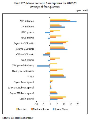 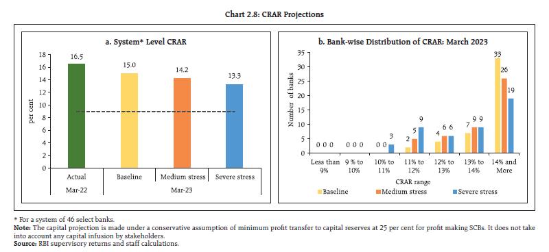 2.18 The common equity Tier I (CET 1) capital ratio of the select 46 SCBs may decline from 13.4 per cent in March 2022 to 12.2 per cent by March 2023 under the baseline scenario (Chart 2.9 a). Even in a severely stressed macroeconomic environment, the aggregate CET1 capital ratio would deplete only by 260 basis points, which would not breach the minimum regulatory norms. Furthermore, all these banks would be able to meet the minimum regulatory CET1 ratio of 5.5 per cent over the next one year under all the three scenarios (Chart 2.9 b). 2.19 Support measures provided by the regulator during the COVID-19 pandemic aided in arresting GNPA ratios of SCBs even with the winding down of regulatory reliefs. Under the assumption of no further regulatory reliefs as well as without taking the potential impact of stressed asset purchases by National Assets Reconstruction Company Limited (NARCL) into account, stress tests indicate that GNPA ratio of all SCBs may improve from 5.9 per cent in March 2022 to 5.3 per cent by March 2023 under the baseline scenario driven by higher expected bank credit growth and declining trend in the stock of GNPAs, among other factors (Chart 2.10). If the macroeconomic environment worsens to a medium or severe stress scenario, the GNPA ratio may rise to 6.2 per cent and 8.3 per cent, respectively. At the bank group level too, the GNPA ratios may shrink by March 2023 in the baseline scenario. In the severe stress scenario, however, the GNPA ratios of PSBs may increase from 7.6 per cent in March 2022 to 10.5 per cent a year later whereas it would go up from 3.7 per cent to 5.7 per cent for PVBs and 2.8 per cent to 4.0 per cent for FBs over the same period. 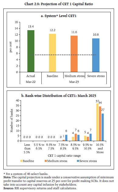
 2.20 Under housing loans, the financed property is generally the underlying collateral and hence, any fall in prices may have implications for lending banks. Accordingly, in the Indian case, house prices were subjected to shocks and it was found that even after a substantial price fall, the system level CRAR would remain well above the regulatory requirement of 9 per cent. At individual bank level, however, shocks of 55 per cent, 60 per cent and 80 per cent fall in the collateral value can result in the capital of one, two and three banks, respectively, to decline below the regulatory limit (Box 2.1). Box 2.1: Housing Price and Financial Stability – Sensitivity Analysis The global financial crisis (GFC) of 2008 underscored the role of a steep drop in housing prices in exacerbating stress in the financial system. The resilience of top Indian scheduled commercial banks (SCBs) to prolonged drops in house prices is tested, using account level data unlike the macro stress test presented earlier. The housing sector is looked at in isolation and only property prices are subjected to shocks but in a conservative stance. With sales growth in the housing market turning positive in Q2:2021-22, housing loan numbers have maintained double-digit growth (Chart 1 a). On the other hand, the growth in housing prices, as measured by the all-India house price index (HPI) of the Reserve Bank, remains below 5 per cent and presently sits at 1.8 per cent (Chart 1 b). With waivers being discontinued and with interest rates rising, the growth in house sales has lost momentum and inventory overhang is still well over 36 months. A sensitivity analysis of the impact of the fall in housing prices on the capital of banks with outstanding mortgages is conducted in line with the methodology of Banco Central do Brasil and Bank Negara Malaysia. The analysis is based on loan-level data till March 2022 obtained from the Residential Asset Price Monitoring Survey (RAPMS). The house property (for which the loan has been availed) is taken as the collateral. The present value of the collateral is estimated by using the change in HPI since the time of origination of the loan. The rate of interest of each housing loan is arrived at by using its sanctioned amount, tenor and equated monthly instalment (EMI). It is then used to arrive at the outstanding amount under the assumption that all EMIs until date have been paid in full. The estimated collateral value is then subjected to price shocks, simulating a sequence of decreases in steps of five percentage points each. Loans for which the shocked collateral value becomes lower than the amount outstanding are considered delinquent. Although collateral falling below the amount outstanding may not result in loans becoming NPAs, a sustained house price fall is considered to factor in capital losses by making allowance for provisions and income loss equivalent to a sub-standard loan. For non-delinquent loans there would be an increase in risk due to increase in the loan-to-value (LTV) ratio. Hence risk-weighted assets (RWA) for them are adjusted upwards using the internal rating based (IRB) formula (Annex 2). Simulations of reductions in residential property prices show a very small possibility of non-compliance to regulatory capital. Even in the event of substantial drop in the collateral value, system level capital to risk-weighted assets ratio (CRAR) will remain well above the regulatory requirement of 9 per cent. Taken individually, all 20 banks under study are able to maintain CRARsabove 9 per cent in response to a shock, up to theextent of 55 per cent on collateral value. Thereafter,a maximum of three banks with large housing loanportfolios face a decline of CRAR below the prescribedminimum under different price shock scenarios(Chart 2).
The analysis reveals that the impact of house price shock on banks’ CRAR may not be significant to cause financial instability even when a sustained fall in prices is considered. Strong capital position of the banks and the fact that housing loan portfolio constitutes only around 15 per cent of SCBs loan portfolio are the key mitigants. References: 1. Banco Central do Brasil (2021). Financial Stability Report, October 2. Bank Negara Malaysia (2019). Financial Stability Review, Second Half 2019. 3. Reserve Bank of India (2019): Residential Asset Price Monitoring Survey (July 11) | II.1.7 Sensitivity Analysis10 2.21 Top-down11 sensitivity analysis involving several single-factor shocks to simulate credit, interest rate, equity price and liquidity risks have been carried out under various stress scenarios12 to assess the vulnerabilities of SCBs, based on their operations up to March 2022. a. Credit Risk 2.22 Credit risk sensitivity has been analysed under two scenarios, in which the system-level GNPA ratio is assumed to rise by (i) one SD13 and (ii) two SD from its prevailing level in a quarter. Under a severe shock of two SD, the GNPA ratio of 46 select SCBs moves up from 6.0 per cent to 11.5 per cent, the system-level CRAR declines from 16.5 per cent to 12.6 per cent and the Tier-1 capital ratio falls from 14.4 per cent to 10.5 per cent. The system-level capital impairment could be 25.2 per cent under the severe shock (Chart 2.11 a). A reverse stress test shows that it requires a shock of 4.7 SD to bring down the system-level CRAR to the regulatory minimum of 9 per cent. 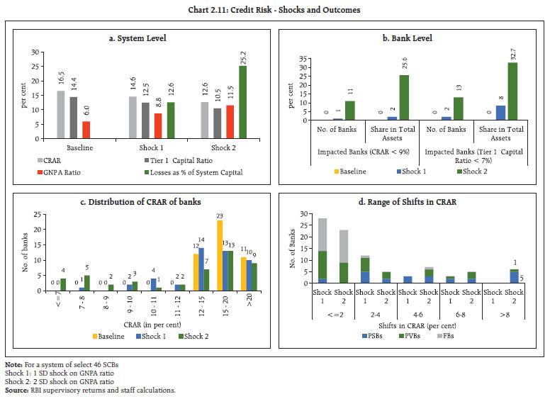 2.23 Bank-level stress test results show that under the severe (two SD shock) scenario, 11 banks with a share of 25.6 per cent in SCBs’ total assets, fail to maintain the regulatory minimum level of CRAR (Chart 2.11 b). In such a scenario, the CRAR falls below 7 per cent in case of four banks (Chart 2.11 c) and six banks record a decline of over eight percentage points in their CRARs. In general, PVBs and FBs face lower CRAR erosion than PSBs under both scenarios (Chart 2.11 d). b. Credit Concentration Risk 2.24 Stress tests on banks’ credit concentration - considering top individual borrowers according to their standard exposures – show that in the extreme scenario of the top three individual borrowers of respective banks failing to repay14, no bank would face a situation of the CRAR falling below the regulatory minimum, although three banks experience a decline of more than five percentage points in their CRARs (Chart 2.12 a and b). 2.25 Under the extreme scenario of the top three group borrowers in the standard category failing to repay15, the CRARs for all banks remain above 11 per cent, though two banks experience more than five percentage points decline in the CRAR (Chart 2.13 a and b).
2.26 In the extreme scenario of the top three individual stressed borrowers of respective banks failing to repay16, a majority of the banks experience a reduction of 25 bps or less in their CRAR (Chart 2.14). c. Sectoral Credit Risk 2.27 Shocks applied on the basis of volatility of industry sub-sector wise GNPA ratio indicate varying magnitudes of increases in banks’ GNPAs in different sub-sectors. A two SD shock to the energy and metals segments reduces the system-level CRAR by 16 bps and 13 bps, respectively (Table 2.2). Table 2.2: Decline in System Level CRAR
(basis points, in descending order for top 10 most sensitive sectors) | | | 1 SD | 2 SD | | Infrastructure - Energy (112%) | 8 | 16 | | Basic Metal and Metal Products (205%) | 8 | 13 | | Infrastructure - Transport (42%) | 3 | 6 | | Construction (53%) | 2 | 4 | | Food Processing (46%) | 2 | 4 | | Infrastructure - Communication (29%) | 1 | 3 | | Gems and Jewellery (29%) | 1 | 3 | | Cement and Cement Products (153%) | 1 | 2 | | Petroleum (non-infra), Coal Products (non-mining) and Nuclear Fuels (78%) | 1 | 2 | | Mining and Quarrying (164%) | 1 | 2 | Note: For a system of select 46 banks.
Numbers in parentheses represent the growth in GNPA of that sub-sector due to 1 SD shock to the sub-sector’s GNPA ratio.
Source: RBI supervisory returns and staff calculations. | d. Interest Rate Risk 2.28 The market value of investments subject to fair value for the sample of SCBs under review stood at ₹18.9 lakh crore in March 2022 (Chart 2.15). 94.8 per cent of these investments were classified as ‘available for sale (AFS)’ and the remaining were under the ‘held for trading (HFT)’ category. PSBs hold more than half of the total trading book portfolio of SCBs, though their share has come down in the recent period. 2.29 The sensitivity (PV0117) of the AFS portfolio increased minimally across bank groups vis-à-vis the December 2021 position, reflecting higher reliance on active interest rate risk management by banks. In terms of PV01 curve positioning, the tenor-wise distribution of PSBs’ portfolio indicated marginally higher allocation in the 5-10 year, paring the allocation to the ‘less than 1-year’ bucket. PVBs have built up investments/allocation in the ‘less than 1-year’ bucket and ‘more than 10-year’ bucket. FBs have continued to prefer the ‘more than 10-year’ bucket, while increasing their positioning marginally in the ‘5-10 year’ bucket. Although PV01 exposure of FBs in the highest maturity segment remains substantial, it may not be an active contributor to risk as some positioning involves bonds held as cover for hedging derivatives (Table 2.3). 2.30 As on June 8, 2022, yields have moved up across the curve relative to December 2021, with the upward shift being more pronounced at the shorter end. This can be attributed to sustained building up of inflation pressures, prevailing geopolitical turmoil and accelerated monetary policy normalisation. As compared to December 2021, the yield curve was flatter by March 2022, the upward shift being more prominent up to 12 years as well as at the longer end of the curve. The spike in the short end of the curve may be ascribed to the increased usage of variable rate reverse repo (VRRR) (Chart 2.16). 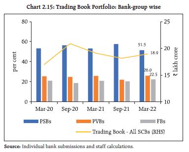
| Table 2.3: Tenor-wise PV01 Distribution of AFS Portfolio | | | Total (in ₹ crore) | Share (in per cent) | | <1 year | 1-5 year | 5-10 year | >10 years | | PSBs | 215.3 (211.8) | 7.0 (8.7) | 39.5 (39.3) | 43.7 (42.2) | 9.8 (9.8) | | PVBs | 61.3 (58.6) | 23.7 (16.3) | 50.0 (55.3) | 12.2 (14.5) | 14.1 (13.8) | | FBs | 137.7 (135.1) | 2.8 (4.1) | 22.5 (22.2) | 16.7 (15.7) | 58.0 (58.0) | Note: Values in the parentheses indicate December 2021 figures
Source: Individual bank submissions and staff calculations |
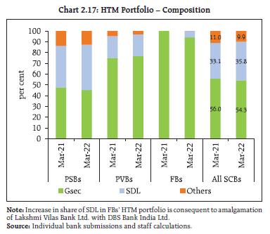
2.31 Trading profit of banks has recorded a marked reduction after Q1:2021-22. During Q4:2021:22, it fell by 17 per cent on a q-o-q basis for PSBs, while it increased for PVBs. FBs continued to report trading losses for the fifth consecutive quarter, with trading losses increasing in Q4:2021-22. The share of trading profits in net operating income declined to low single digits for both PSBs and PVBs (Table 2.4). There was also a rebound in other operating income (OOI) beyond pre-pandemic levels. 2.32 The interest rate exposure of PVBs and FBs in their HFT portfolios remained higher than that of PSBs, with PSBs having an overall short position in their HFT books, where short positions were built up in ‘less than 1-year’ and ‘more than 10-year’ buckets. Banks diverged in their trading strategies and interest rate outlook: PSBs had pronounced short positions in the more than 10-year bucket, while PVBs were long in all buckets and FBs were marginally short in the less than 1-year bucket (Table 2.5). 2.33 Any hardening of interest rates would depress investment income under the AFS and HFT categories (direct impact). It is assessed that a parallel upward shift of 250 bps in the yield curve would reduce the system level CRAR by 80 bps to 15.70 per cent. Analogously, the system level CET I capital would decline by 83 bps to 12.57 per cent (Table 2.6). 2.34 During 2021-22, PSBs preferred to augment their allocation in SDLs and wind down their other holdings in the HTM category (Chart 2.17). Under the then prevailing low interest rate conditions, banks sold a large portion of their HTM portfolio and booked profits, The outstanding HTM portfolio as on March 31, 2022, has relatively the same proportion of unrealised gains from SDLs and unrealised losses from G-Secs (Chart 2.18). Since G-Secs form the largest share of the HTM portfolio, the presence of substantial unrealised losses, especially in respect of PSBs, at the beginning of the interest rate tightening cycle, portends risk to their financial health going forward. | Table 2.4: OOI - Profit/(Loss) on Securities Trading | | (in ₹ crore) | | | Q4: 2020-21 | Q1: 2021-22 | Q2: 2021-22 | Q3: 2021-22 | Q4: 2021-22 | | PSBs | 5104 (9.1) | 9024 (17.7) | 5765 (13.9) | 3023 (6.4) | 2507(4.7) | | PVBs | 2499 (5.4) | 3669 (7.7) | 1996 (4.4) | 573 (1.2) | 1155 (2.3) | | FBs | -223 (-1.9) | -417 (-4.3) | -204 (-2.6) | -874 (-11.2) | -2183 (-20.3) | Note: Figures in parentheses represent OOI-Profit/(Loss) as a percentage of Net Operating Income.
Source: RBI Supervisory Returns |
| Table 2.5: Tenor-wise PV01 Distribution of HFT portfolio | | | Total (in ₹ crore) | Share (in per cent) | | <1 year | 1-5 year | 5-10 year | >10 years | | PSBs | -0.04 (1.5) | -12.7 (0.7) | 180.0 (13.6) | 161.1 (27.6) | -228.4 (58.2) | | PVBs | 14.4 (8.0) | 1.8 (2.4) | 5.7 (16.1) | 92.0 (14.1) | 0.4 (68.1) | | FBs | 7.5 (9.4) | -9.2 (-5.0) | 14.4 (23.2) | 74.3 (29.4) | 20.5 (52.4) | Note: Values in the brackets indicate December 2021 figures.
Source: Individual bank submissions and staff calculations. |
Table 2.6: Interest Rate Risk – Bank-groups - Shocks and Impacts
(under shock of 250 basis points parallel upward shift of the INR yield curve) | | | Public Sector Banks | Private Sector Banks | Foreign Banks | All SCBs | | AFS | HFT | AFS | HFT | AFS | HFT | AFS | HFT | | Modified Duration | 2.2 | -1.3 | 1.3 | 4.1 | 3.8 | 1.2 | 2.3 | 2.2 | | Reduction in CRAR (bps) | 77 | 35 | 301 | 80 | | Reduction in CET-I Capital (bps) | 81 | 36 | 308 | 83 | | Source: Individual bank submissions and staff calculations. |
 2.35 In March 2022, holding of SLR securities by PSBs and PVBs in the HTM category amounted to 21.0 per cent and 18.2 per cent of their NDTL, respectively, while it stood at 1.1 per cent for FBs. Taking advantage of the special dispensation permitting banks to classify SLR securities acquired between September 2020 and March 2022, under the HTM category, banks increased their HTM portfolio by 9 per cent during 2021-22. With PSBs’ HTM holdings approaching their regulatory threshold, the enhancement in HTM limit to 23 per cent of NDTL for securities acquired between April 1, 2022 and March 31, 2023 would enable banks to better manage their investment portfolio. e. Equity Price Risk 2.36 An analysis of the possible impact of a significant fall in equity prices on banks’ CRAR indicates that equity price risk is limited for the overall system as banks have low proportion of capital market exposures due to regulatory limits. Under the scenarios of 25 per cent, 35 per cent and 55 per cent drops in equity prices, the system level CRAR would decline by 21 bps, 30 bps and 47 bps, respectively (Chart 2.19). f. Liquidity Risk 2.37 Liquidity risk analysis aims to capture the impact of a possible run on un-insured deposits18 and potential increase in demand for unutilised portions of sanctioned/committed/guaranteed credit lines.
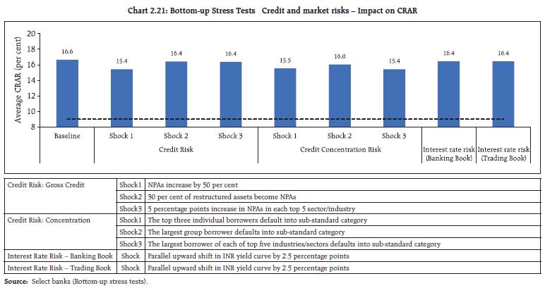
2.38 In a scenario of sudden and unexpected withdrawals of around 15 per cent of un-insured deposits along with the utilisation of 75 per cent of unutilised portion of committed credit lines, liquid assets19 at the system level as a percentage of total assets will decrease to 12.4 per cent from 21.9 per cent (Chart 2.20). II.1.8 Bottom-up Stress Tests: Credit, Market and Liquidity Risk 2.39 A series of bottom-up stress tests (sensitivity analyses) has been conducted for select banks20 with the reference date of March 31, 2022. The results testify to banks’ general resilience to different kinds of shocks and are generally in line with the findings from the top-down stress tests. Under different stress scenarios, the CRAR of all banks would remain above the regulatory minimum of 9 per cent. Average CRAR of banks is found to be higher than under a similar stress test exercise conducted a year ago with March 31, 2021 as the reference date (Chart 2.21). 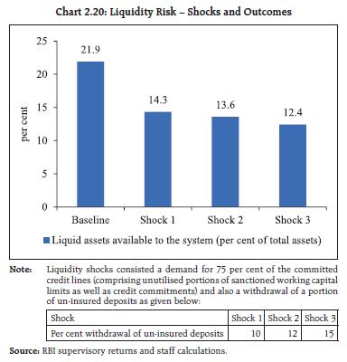
 2.40 The bottom-up stress tests for liquidity risk performed on select banks indicate that they would have positive liquid assets ratios21 under various alternative scenarios. HQLAs would enable banks in the sample to withstand liquidity pressures from sudden and unexpected withdrawal of deposits in each scenario. Under both scenarios, average liquid assets ratios of the select banks are found to be lower than those obtained under a similar exercise a year ago (Chart 2.22). II.1.9 Bottom-up Stress Tests: Derivatives Portfolio 2.41 A series of bottom-up stress tests (sensitivity analyses) on derivative portfolios have been conducted for select banks22 with the reference date as March 31, 2022. The derivative portfolios of the banks in the sample are subjected to four separate shocks on interest and foreign exchange rates. While the shocks on interest rates ranged from 100 to 250 basis points, a 20 per cent appreciation/depreciation shocks of foreign exchange rates is assumed. The stress tests are carried out for individual shocks on a stand-alone basis. 2.42 Most of the FBs maintain significantly negative net mark-to-market (MTM) positions as a proportion of CET-1 capital in March 2022. The MTM impact is by and large, muted for PSBs and PVBs (Chart 2.23).
2.43 The derivative portfolios of the sample banksare positioned to gain from an interest rate rise andvice versa. Potential MTM gains from a rise in interestrates has amplified in March 2022 as compared withthe September 2021 position. Going forward, MTMgains for derivatives portfolio are expected to risefurther against the backdrop of a rising interestrate regime. Contrary to interest rate shocks,the net impact of both the foreign exchange rate shocks remained subdued in the last two quarters (Chart 2.24). II.2 Small Finance Banks 2.44 The universe of small finance banks (SFBs) form 1.0 per cent of total assets of the SCBs. Aggregate deposits and credit of SFBs increased by 32.7 per cent and 23.1 per cent, respectively, during the four quarters of 2021-22 (quarterly average y-o-y growth). SFBs have been aggressively increasing their CASA deposits, with their share in total deposits increasing from 18.4 per cent in March 2019 to 33.9 per cent in March 2022 even as term deposits recorded a growth of 15.7 per cent (y-o-y) in March 2022 (Chart 2.25 a). 2.45 The high balance sheet growth of SFBs from a low base has raised some concerns on asset quality: their restructured standard advances portfolio remains higher than pre-pandemic levels, though below the peak of September 2021 (Chart 2.25 b).
The concentration of SFBs to limited geographies and customer profiles are factors influencing these developments. Their CRAR, however, remains comfortable at 19.3 per cent in March 2022, which is higher than the larger group of SCBs, though their PCR at 53.9 per cent stood significantly lesser than other banking groups in the SCB cohort (Chart 2.25 c). The RoE and RoA numbers had slipped into negative zone in September 2021. These ratios have, however, recorded a turnaround in H2:2021-22 but remain lower than historical trends (Chart 2.25 d). II.3 Primary (Urban) Cooperative Banks 2.46 Priority sector lending23 of primary (urban) cooperative banks (UCBs)24 crossed the March 31, 2022 target of 50 per cent and is nearing the March 31, 2023 target of 60 per cent (Chart 2.26 a). The CRAR of UCBs improved during H2:2021-22 to reach 15.8 per cent in March 2022. The CRAR of scheduled UCBs (SUCBs) improved to 14.4 per cent primarily because of the amalgamation of one UCB with an SFB (Chart 2.26 b).
2.47 After a sudden spike in September 2021 caused by the second wave of COVID-19, GNPA ratios of both SUCBs and NSUCBs improved significantly to 7.4 per cent and 11.3 per cent, respectively, by March 2022 (Chart 2.26 c). Their NNPA ratios also moderated during the year (Chart 2.26 d). Though provisions declined, PCR of SUCBs and NSUCBs improved to 64.9 per cent and 62.2 per cent, respectively, due to large fall in their GNPAs (Chart 2.26 e). UCBs recorded improvement in profitability in terms of NIM, RoA and RoE ratios during 2021-22 (Chart 2.26 f, g and h). II.3.1 Stress Testing 2.48 Stress tests have been conducted on a select set of UCBs25 to assess credit risk (default risk and concentration risk), market risk (interest rate risk in trading book and banking book) and liquidity risk, based on their reported financial positions as of March 2022. 2.49 The results show that (a) a few UCBs fail on four of the five parameters even in the baseline scenario; (b) the impact of credit default risk is higher than credit concentration risk in all three scenarios; (c) the impact of shock to the trading book and the banking book is minimal; (d) liquidity shocks impact the largest number of UCBs (Chart 2.27). II.4 Non-Banking Financial Companies26 (NBFCs) 2.50 Aggregate credit extended by NBFCs stood at ₹28.5 lakh crores in March 2022. Loans to industry constituted the largest segment (39.1 per cent), followed by personal loans (27.4 per cent) and those to services (15.3 per cent). Credit to agriculture sector accounted for a miniscule share (1.8 per cent) (Chart 2.28). Government owned NBFCs accounted for 45.6 per cent of aggregate credit extended by all NBFCs (Chart 2.29). Their dominant share of over three fourths of the industrial loans has, however, been receding (Chart 2.30).
2.51 In terms of credit dispensation by category of NBFC, investment and credit companies (NBFC-ICC) and infrastructure finance companies (NBFC-IFC) predominated in gross loans and advances in March 2022 (Chart 2.31). 2.52 The GNPA ratio of NBFCs eased in March 2022 from 6.8 per cent in September 2021, the moderation witnessed across both public and private sector NBFCs. The improvement was primarily on account of 340 bps dip in the GNPA ratio of the services sector. Nevertheless, it remained higher than other sectors at 9.9 per cent. There was a larger concentration of NPAs in the industrial sector for which the loan book size far exceeds that of the services sector (Chart 2.32). The aggregate NNPA ratio of NBFCs also ebbed in March 2022, despite a 90 bps rise in the NNPA ratio for the industrial sector loans on account of curtailed provisioning (Chart 2.33). The capital position of NBFCs remained robust and their return on assets (RoA) recouped in March 2022 (Chart 2.34).
2.53 Borrowings remained the major source of funds for NBFCs (Chart 2.35), mainly in the form of debentures and bank borrowings (Chart 2.36).
II.4.1 Stress Test27 - Credit Risk 2.54 The resilience of NBFC sector to credit risk shocks has been assessed for a sample of 155 NBFCs28 under a baseline and two stress scenarios – medium and high risk, with increase in the slippage ratio by 1 SD and 2 SD, respectively. The capital adequacy ratio of the sample NBFCs was at 26.7 per cent and GNPA ratio at 4.6 per cent in March 2022. The baseline scenario projected holds for one year ahead from this reference date, based on assumptions of business continuing under usual conditions. 2.55 Under the baseline scenario, the CRAR of nine NBFCs – comprising 1.72 per cent of total advances of the sample companies – is less than the minimum regulatory requirement of 15 per cent. Under a medium risk shock of a 1 SD increase in the slippage ratio, the GNPA ratio rises to 6.73 per cent and the resultant income loss and additional provisional requirements reduce the CRAR by 50 bps to 23.83 percent with CRARs of twelve NBFCs falling below 15 per cent. Under the high-risk shock of 2 SD increase in the slippage ratio, the GNPA ratio increases to 9.39 per cent, the capital adequacy ratio of the sector declines by 82 bps to 23.51 per cent and CRAR of fifteen NBFCs falls below minimum regulatory requirements (Chart 2.37). II.4.2 Stress Test - Liquidity Risk 2.56 The resilience of the NBFC sector to liquidity shocks is assessed by capturing the impact of a combination of assumed increase in cash outflows and decrease in cash inflows29. The baseline scenario uses the projected outflows and inflows as of March 2022. One baseline and two stress scenarios are applied – a medium risk scenario involving a shock of 5 per cent contraction in inflows and 5 per cent rise in outflows; and a high risk scenario entailing a shock of 10 per cent decline in inflows and 10 per cent surge in outflows. The results indicate that the number of NBFCs which would face negative cumulative mismatch in liquidity positions over the next one year in the baseline, medium and high-risk scenarios stood at 10 (representing 4.6 per cent of asset size of the sample), 23 (8.6 per cent) and 40 (21.5 per cent), respectively (Table 2.7). 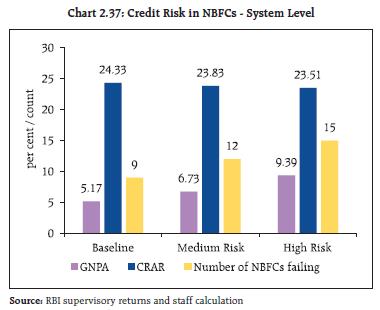
| Table 2.7: Liquidity Risk in NBFCs | | Cumulative Mismatch as a percentage of outflows over next one year | No. of NBFCs having liquidity mismatch | | Baseline | Medium | High | | Over 50 per cent | 3 (0.2) | 4 (0.2) | 4 (0.2) | | Between 20 and 50 per cent | 4 (1.0) | 4 (2.8) | 12 (5.7) | | 20 per cent and below | 3 (3.4) | 15 (5.6) | 24 (15.6) | Note: Figures in parenthesis represent percentage share in asset size of the sample
Source: RBI supervisory returns and staff calculations. | II.5 Interconnectedness 2.57 A financial system can be visualised as a network with financial institutions as nodes and bilateral exposures as links joining these nodes. These links which could be in the form of loans to, investments in, or deposits with each other act as a source of funding, liquidity, investment and risk diversification, but could also transform in adverse conditions into channels through which shocks can spread, leading to contagion and amplification of systemic shocks. Understanding the nuances of such networks becomes critical for safeguarding macroeconomic and financial stability. II.5.1 Financial System Network30 31 2.58 The total outstanding bilateral exposures32 among the entities in the financial system maintained steady growth. A major part of the surge emanated from higher funding requirements of PVBs (Chart 2.38 a). The increase in the March 2022 quarter was primarily due to higher exposure of SCBs to the financial system and of All-India Financial Institutions (AIFIs) and asset management companies (mutual funds) (AMC-MFs) to SCBs (Chart 2.38 b). 2.59 SCBs had the largest share of bilateral exposures. The shares of NBFCs, HFCs and insurance companies declined on a sequential and on y-o-y basis. Owing to the correction in the equity markets, the share of AMC-MFs in bilateral exposures contracted sharply from 13.4 per cent in September 2021 to 12.5 per cent in December 2021 before rising marginally in Q4:2021-22 (Chart 2.38 b). 2.60 In terms of inter-sectoral33 exposures, AMC-MFs, followed by insurance companies, were the biggest fund providers in the system, whereas NBFCs and HFCs were the largest receivers of funds, followed by PVBs. Among the bank groups, PSBs and UCBs had net receivable positions vis-à-vis the entire financial sector whereas PVBs, SFBs and FBs had net payable positions (Chart 2.39). 2.61 Net receivables of AMC-MFs and PSBs from the financial system increased during 2021-22. Among recipients of funds from the financial system, PVBs recorded a large increase while payables of NBFCs and HFCs also increased during the period34 (Chart 2.40). a. Inter-bank Market 2.62 Inter-bank exposures accounted for 3.1 per cent of the total assets of the banking system as of March 2022, with fund-based exposure constituting the major part (2.5 per cent). In absolute terms, both fund-based35 and non-fund-based exposures (primarily letters of credit and bank guarantees)36 bounced back to reach their pre-pandemic levels (Chart 2.41).
2.63 PSBs continued to maintain a dominant position in the inter-bank market and their share increased both on sequential and annual bases. The share of PVBs increased on a sequential basis, whereas that of FBs fell during Q4:2021-22 (Chart 2.42). 2.64 About 74 per cent of the fund-based interbank market was short-term (ST) in nature in which ST deposits had the highest share, followed by ST loans and call money market exposure. Long-term (LT) loans predominated in LT fund-based interbank exposures (Chart 2.43).
b. Inter-bank Market: Network Structure and Connectivity 2.65 The inter-bank market typically has a core-periphery network structure37 38. As of end-March 2022, four banks were in the inner-most core and five banks in the mid-core circle. The four banks in the inner-most core included a large public and three private sector banks. The banks in the mid-core were PSBs and PVBs. Most of the old PVBs along with FBs, SUCBs and SFBs formed the periphery (Chart 2.44). 2.66 The degree of interconnectedness in the banking system (SCBs), as measured by the connectivity ratio39 continued to decline over the year. Smaller FBs do not actively participate in the inter-bank market. The rise in their local interconnectedness through tendency to cluster, however, intensified as reflected in the increase in cluster coefficient to 42.6 per cent in March 2022 from 39.4 per cent a year ago (Chart 2.45). c. Exposure of AMC-MFs 2.67 In terms of inter-sectoral exposures, AMC-MFs maintained their position as the largest net providers of funds to the financial system as of end 2021-22. Their gross receivables stood at ₹11.41 lakh crore (around 31 per cent of their average AUM) whereas their gross payables were ₹0.93 lakh crore as at end- March 2022. SCBs were the major recipients of their funding. The momentum of AMC-MF exposure to banking sector has been rising since June 2020, exceeding pre-pandemic levels by Q4:2021- 22. Their receivables from AIFIs also increased (Chart 2.46 a). 2.68 The asset composition of AMC-MFs witnessed a significant shift in Q4:2021-22. The share of equity holdings in AMC-MFs receivables declined in Q4:2021-22 with the meltdown in the equity market. Furthermore, the share of long-term (LT) debt underwent a sharp markdown sequentially. On the other hand, their exposure to CDs surged from 6 per cent to 15 per cent in Q4:2021-22 (Chart 2.46 b).
d. Exposure of Insurance Companies 2.69 Insurance companies were the second largest net providers of funds to the financial system, with gross receivables at ₹7.29 lakh crore and gross payables at ₹0.46 lakh crore in March 2022. SCBs were the largest recipients of their funds, followed by subscription to LT debt issued by NBFCs and HFCs, and equity (Chart 2.47 a and b). e. Exposure to AIFIs 2.70 AIFIs were net borrowers of funds from the financial system, their gross payables and gross receivables having increased to ₹5.19 lakh crore and ₹4.77 lakh crore, respectively, in March 2022. They raised funds mainly from SCBs (primarily PVBs), AMC-MFs and insurance companies (Chart 2.48 a). Given their nature of operations, LT debt and LT deposits remained their preferred instruments for raising funds but the combined share of these instruments has declined to 41.5 per cent from 52.7 per cent a year ago, and they mobilised funds through CPs and CDs in Q4:2021-22 (Chart 2.48 b). f. Exposure to NBFCs 2.71 NBFCs were the largest net borrowers of funds from the financial system, with gross payables of ₹12.46 lakh crore and gross receivables of ₹1.62 lakh crore as at end-March 2022. Over half of their borrowings were from SCBs and this share increased further during H2:2021-22 as their reliance on funding by AMC-MFs and insurance companies reduced. (Chart 2.49 a). Instrument wise, the NBFC funding mix saw a rise in LT loans whereas the share of LT debt instruments and CPs declined during 2021-22 (Chart 2.49 b).
g. Exposure to HFCs 2.72 HFCs were the second largest net borrowers of funds from the financial system, with gross payables of ₹7.40 lakh crore and gross receivables of ₹0.63 lakh crore as at end-March 2022. As in the case of NBFCs, the reliance of HFCs on funding from SCBs has been high and it rose further during the year. Their share of borrowings from AMC-MFs declined while the share of insurance companies has remained largely stable (Chart 2.50 a). The proportion of resource mobilisation through LT debt instruments has contracted since March 2021 while loans (both LT and ST) grew on an annual as well as sequential basis. The share of funds mobilised through CPs varied through the year (Chart 2.50 b). III.5.2 Contagion Analysis 2.73 Contagion analysis uses network technology to estimate the systemic importance of individual banks. The failure of a systemically important bank leads to solvency and liquidity losses for the banking system, the scale of which depends on the capital and liquidity positions of banks as well as the extent and nature of exposure (whether it is a lender or a borrower) and magnitude of the interconnections that the failing bank has with the rest of the banking system. a. Joint Solvency40-Liquidity41 Contagion Losses for SCBs due to Bank Failure 2.74 A contagion analysis of the banking network, based on the end-March 2022 position, indicates that the bank with the maximum capacity to cause contagion losses (Table 2.8) is positioned in the inner-most core of the core-periphery network structure (Chart 2.44) and its failure would lead to a solvency loss of 2.83 per cent of the total Tier 1 capital of SCBs and liquidity loss of 0.02 per cent of total HQLA of the banking system. 2.75 An analysis of the five banks with the maximum capacity to cause contagion losses shows that possible contagion losses due to their failure increased in March 2022 vis-à-vis September 2021, which may be attributed to the deepening of the inter-bank market during the interregnum. | Table 2.8: Contagion Losses due to Bank Failure – March 2022 | | Trigger Code | % of Tier 1 capital of the Banking System | % of HQLA | Number of Bank defaulting due to solvency | Number of Bank defaulting due to liquidity | | Bank 1 | 2.83 | 0.02 | 0 | 0 | | Bank 2 | 2.31 | 0.20 | 0 | 0 | | Bank 3 | 2.16 | 0.01 | 0 | 0 | | Bank 4 | 1.83 | 0.12 | 0 | 0 | | Bank 5 | 1.82 | 0.50 | 0 | 0 | Note: ‘Trigger banks’ have been selected on the basis of solvency losses caused to the banking system.
Source: RBI supervisory returns and staff calculations. | 2.76 The presence of banks with traditionally strong deposit franchise businesses in this cohort is indicative of rising credit growth and increased reliance on the inter-bank market. This, however, would not lead to the failure of any additional bank on solvency and liquidity criteria (Table 2.8 and Box 2.2). Box 2.2: Determinants of solvency contagion loss due to bank failure The international transmission of financial shocks post Global Financial Crisis has highlighted the importance of analysis of contagion channels. The extent of loss that could be triggered by a financial institution is also an indicator of its systemic importance. Global systemically important banks (G-SIBs) are also required to maintain additional capital buffers to reduce their probability of failure and its impact on the system (BCBS, 2018). The FSR regularly makes assessments of contagion losses of the banking system due to failure of banks, NBFCs and HFCs and the results of hypothetical scenarios of failure of top five entities in each category having the maximum capacity to cause contagion losses are released on a half yearly basis. In order to ascertain the factors influencing the extent of solvency contagion loss at a system level due to idiosyncratic failure of the top-most bank having the maximum capacity to cause such loss, two alternative autoregressive distributed lag (ARDL) models are estimated for the dependent variable (ratio of solvency contagion loss due to failure of the top-most bank to cause maximum loss to Tier 1 capital of the banking system) with the regressor variables being (i) ratio of inter-bank exposure to total bank assets; (ii) tier 1 capital ratio and (iii) connectivity ratio (which measures actual number of links relative to maximum possible number of links). Quarterly data from March 2017 to March 2022 are used for which stationarity and bounds test conditions were satisfied for applying the ARDL model (Pesaran, Shin and Smith, 2001). | Table 1: Estimated models | | Variables | Model 1 ARDL(1,1,0) | Model 2 ARDL(1,0,0,1) | | Coefficient | t-statistic | Coefficient | t-statistic | | Dependent variable (-1) | -0.092 | -0.779 | -0.071 | -0.555 | | Inter-bank exposure to total bank assets | 3.573** | 2.461 | 5.559*** | 3.305 | | Inter-bank exposure to total bank assets (-1) | -3.235 | -1.597 | | | | Tier 1 capital ratio | -2.587** | -2.268 | -4.496** | -2.274 | | Connectivity ratio | | | 0.185 | 0.337 | | Connectivity ratio (-1) | | | 1.326* | 1.770 | | Constant | 38.460* | 1.938 | -30.535 | -1.109 | | @Trend | | | 1.564** | 2.300 | | Regression Diagnostics: | | | | | | Adj. R-square | 0.605 | | 0.649 | | | Durbin-Watson statistic | 2.496 | | 2.093 | | | F-statistic | 8.660*** | | 7.155*** | | | Serial correlation LM test p-value | 0.386 | | 0.943 | | | BPG Heteroskedasticity test p-value | 0.267 | | 0.292 | | | Correlogram of residuals and squared residuals are insignificant for both the models. | | | | | Bounds Test:
F-statistic (Null: No levels relationship) | 17.646*** | | 16.862*** | | | Note *, ** and *** denote significance at 10%, 5% and 1% level, respectively. | The results suggest that solvency contagion loss is driven by inter-bank market size, banks’ capital ratios and connectivity ratios – higher inter-bank exposure or interconnectedness leads to higher solvency contagion loss while better capital positions reduce the loss (Table 1). In the long run, only Tier-1 capital ratio is significant as per model 1, whereas both inter-bank exposure and Tier-1 capital ratios are significant as per model 2. One percentage point increase in the inter-bank exposure to total bank assets ratio contributes five percentage point rise in loss whereas, similar increase in Tier 1 capital ratio reduces loss by four percentage point as per model 2 (Table 2). It can thus, be concluded that in order to contain contagion loss, banks need to improve their capital position commensurate with the inter-bank market size and interconnectedness. | Table 2: Levels equation (long-run equation) | | Variables | Model 1 | Model 2 | | Coefficient | t-statistic | Coefficient | t-statistic | | Inter-bank exposure to total bank assets | 0.310 | 0.237 | 5.192*** | 3.313 | | Tier 1 capital ratio | -2.368** | -2.210 | -4.199* | -2.108 | | Connectivity ratio | | | 1.412 | 1.734 | | Constant | 35.213* | 1.873 | | | | @Trend | | | 1.460* | 2.114 | References: 1. BCBS, 2018. Global systemically important banks: revised assessment methodology and the higher loss absorbency requirement, July 2018. 2. Financial Stability Reports, various issues, Reserve Bank of India. 3. Pesaran, MH, Shin, Y., & Smith, R. (2001). Bound testing approaches to the analysis of level relationships. Journal of Applied Econometrics, 16(3), 289–326. | b. Solvency Contagion Losses for SCBs due to NBFC/HFC Failure 2.77 The failure of any NBFC or HFC would also act as a solvency shock to their lenders depending on the extent of exposure, and solvency losses can spread through contagion. 2.78 By end-March 2022, the idiosyncratic failure of an NBFC with the maximum capacity to cause solvency losses to the banking system would have impacted banks’ total Tier-1 capital by 2.40 per cent (as compared with 2.28 per cent in September 2021). In a similar scenario in the HFCs’ domain, the impact of total Tier-I capital would be 5.88 per cent (6.43 per cent in September 2021). In both cases, however, it would not lead to failure of any bank (Tables 2.9 and 2.10). c. Solvency Contagion Impact42 after Macroeconomic Shocks to SCBs 2.79 The contagion from the failure of a bank is likely to get magnified if macroeconomic shocks result in distress to the banking system. In such a situation, similar shocks may cause some SCBs to fail the solvency criterion, which then acts as a trigger for further solvency losses. 2.80 In the previous iteration, the shock was applied to the entity that could cause the maximum solvency contagion losses. In another iteration in which the initial impact of such a shock on an individual bank’s capital is taken from the macro-stress tests43, the initial capital loss due to macroeconomic shocks stood at 8.34 per cent, 12.88 per cent and 18.42 per cent of Tier-I capital for baseline, medium and severe stress scenarios, respectively. No bank fails to maintain Tier-I capital adequacy ratio of 7 per cent in any of the scenarios. As a result, there are no additional solvency losses to the banking system due to contagion (over and above the initial loss of capital due to the macro shocks) (Chart 2.51). | Table 2.9: Contagion Losses due to NBFC Failure – March 2022 | | Trigger Code | Solvency Losses as % of Tier -1 Capital of the Banking System | Number of Banks Defaulting due to solvency | | NBFC 1 | 2.40 | 0 | | NBFC 2 | 1.85 | 0 | | NBFC 3 | 1.75 | 0 | | NBFC 4 | 1.42 | 0 | | NBFC 5 | 1.39 | 0 | Note: Top five ‘Trigger NBFCs’ have been selected on the basis of solvency losses caused to the banking system.
Source: RBI supervisory returns and staff calculations. |
| Table 2.10: Contagion Losses due to HFC Failure – March 2022 | | Trigger Code | Solvency Losses as % of Tier -1 Capital of the Banking System | Number of Banks Defaulting due to solvency | | HFC 1 | 5.88 | 0 | | HFC 2 | 4.88 | 0 | | HFC 3 | 1.64 | 0 | | HFC 4 | 1.41 | 0 | | HFC 5 | 1.13 | 0 | Note: Top five ‘Trigger HFCs’ have been selected on the basis of solvency losses caused to the banking system.
Source: RBI supervisory returns and staff calculations | Summary and Outlook 2.81 Financial entities have generally emerged resiliently from the pandemic and are expanding their business as the economic recovery takes hold. Their asset quality has improved and capital positions remained strong. Macro stress tests reveal that SCBs would be able to withstand adverse macroeconomic circumstances. Also, any negative shock to house prices is not likely to significantly impact banks’ capital positions. Sensitivity analysis shows that credit concentration risk and equity price risk may not be substantial but banks, especially PSBs, having substantial unrealised losses in their books at the beginning of the interest rate tightening cycle, portends risks to their financial health going forward. Network analysis results suggest that contagion losses have increased during H2:2021-22.
|