Scheduled commercial banks’ (SCBs) credit growth remained subdued at 8.7 per cent year-on-year (y-o-y) in September 2019, though private sector banks (PVBs) registered double digit credit growth of 16.5 per cent. SCBs’ capital adequacy ratio improved significantly to 15.1 per cent in September 2019 after the recapitalisation of Public Sector Banks (PSBs) by the Government. SCBs’ gross non-performing assets (GNPA) ratio remained unchanged at 9.3 per cent between March and September 2019. Provision coverage ratio (PCR) of all SCBs rose to 61.5 per cent in September 2019 from 60.5 per cent in March 2019 implying increased resilience of the banking sector. Macro-stress tests for credit risk show that under the baseline scenario, SCBs’ GNPA ratio may increase from 9.3 per cent in September 2019 to 9.9 per cent by September 2020 . This is primarily due to change in macroeconomic scenario, marginal increase in slippages and the denominator effect of declining credit growth. As per network analysis, total bilateral exposures between entities in the financial system registered a marginal decline in quarter ended September 2019. Among all the intermediaries, private sector banks (PVBs) saw the highest y-o-y growth in their payables to the financial system, while insurance companies recorded the highest y-o-y growth in their receivables from the financial system. Commercial paper (CP) funding amongst the financial intermediaries continued to decline in the last four quarters. The size of the inter-bank market continued to shrink with inter-bank assets amounting to less than 4 per cent of the total banking sector assets as at end-September 2019. This reduction, along with better capitalisation of PSBs led to a reduction in contagion losses to the banking system compared to March 2019 under various scenarios relating to idiosyncratic failure of a bank/non-banking finance company (NBFC)/housing finance company (HFC) and macroeconomic distress. Section I Scheduled commercial banks1 2 2.1 This section discusses SCBs’ soundness and resilience under two broad sub-heads: i) performance, and ii) resilience. The latter uses macro-stress tests through scenarios and single-factor sensitivity analyses. Performance 2.2 SCBs’ aggregate credit growth moderated to 8.7 per cent on a y-o-y basis in September 2019 from 13.2 per cent in March 2019; deposit growth improved to 10.2 per cent from 9.9 per cent (Chart 2.1a). The banking sector’s credit growth falling short of deposit growth was last seen during Q2:2016-17. Among bank groups, credit growth of public sector banks (PSBs) decelerated to 4.8 per cent (y-o-y) in September 2019 from 9.6 per cent in March 2019; private sector banks’ (PVBs) credit growth moderated to 16.5 per cent from 21 per cent. There was, however, a sharp contrast between the wholesale and retail credit3 growth in PVBs - wholesale credit grew at 7.2 per cent as against a retail credit growth of 27.2 per cent. Deposit growth in both PSBs and PVBs exceeded their credit growth, although deposit growth in PSBs remained relatively sluggish at 6.6 per cent y-o-y in September 2019 as against 19 per cent for PVBs. 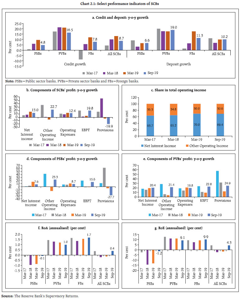 2.3 Growth in net interest income (NII) slowed down to 13 per cent in September 2019 as compared to 16.5 per cent in March 2019, one possible reason being higher growth in deposits as compared to credit. However, due to higher growth in other operating income (OOI) (particularly driven by profits on securities trading in PSBs which increased about tenfold as compared to end-September 2018), SCBs were able to maintain better earnings before provisions and taxes (EBPT) growth (Chart 2.1b). Given that PSBs’ trading portfolio classified as held for trading (HFT) is miniscule, such an increase in profits on securities trading is possibly due to aggressive available for sale (AFS) positioning (paragraph 2.28). However, the AFS portfolio being part of the structural balance sheet typically does not have safeguards like risk limits / stop loss limits which are typically available for pure trading portfolios. Aggressive interest rate positioning in the structural balance sheet based on anticipated softening of rates may have significant adverse consequences if the anticipated rate softening fails to materialise. With regards to buffers against anticipated risks, PVBs’ provisions grew at a faster rate as compared to those of PSBs (Chart 2.1d and e). 2.4 PSBs’ profitability ratios were muted because of weak credit growth as well as slow resolution of non-performing assets (NPAs). PVBs’ profitability ratios also declined whereas foreign banks showed better profitability (Chart 2.1f and g). PSBs’ weak return on equity (RoE) and return on assets (RoA) numbers compared to their private sector counterparts continue to come in the way of their ability to raise equity capital from the market at a decent cost. 2.5 Post the corporate tax rate cut in September 2019, a few banks decided to exercise the option of lower tax rate available under Section 115BAA of the Income Tax Act, 1961. Hence, profit after tax (PAT) across different banks is strictly not comparable for Q2:2019-20 and H1:2019-20 financial results. Concurrently, certain banks have re-measured their accumulated deferred tax assets as on March 31, 2019 based on the lower rate prescribed and the resultant impact has been taken through the profit and loss account (P&L). Comparing the performance in H1:2019-20 across various categories of SCBs using Profit Before Tax (PBT) shows that RoA for PVBs has improved from 1.7 per cent (1.2 per cent based on PAT) as at end-September 2018 to 1.8 per cent (1.0 per cent based on PAT) as at end- September 2019 as opposed to a decrease in RoA based on PAT. For PSBs, RoA based on PBT improved from -1.0 per cent (-0.7 per cent based on PAT) as at end-September 2018 to 0 per cent (-0.1 per cent based on PAT) as at end-September 2019. On an aggregate basis RoA of SCBs based on PBT moved from 0 per cent (-0.004 per cent based on PAT) as at end-September 2018 to 0.7 per cent (0.4 per cent based on PAT) as at end-September 2019. Hence, the improvement in SCBs’ profitability has been more robust than what has been indicated based on PAT figures for Q2:2019-20 after isolating for the one-off charges and the reduced taxation related impact. Asset quality and capital adequacy 2.6 SCBs’ GNPA ratio remained unchanged at 9.3 per cent between March 2019 and September 2019, though the level of GNPAs increased marginally by 0.2 per cent during the same period (Chart 2.2a). However, SCBs’ net non-performing assets (NNPA) ratio declined in September 2019 reflecting increased provisioning (Chart 2.2b). The aggregate provision coverage ratio (PCR) of all SCBs increased to 61.5 per cent in September 2019 from 60.5 per cent in March 2019 (Chart 2.2d). PCRs of both PSBs and PVBs increased in September 2019 (Chart 2.2e). 2.7 Following the recapitalisation of PSBs by the government, SCBs’ capital to risk-weighted assets ratio (CRAR) improved to 15.1 per cent in September 2019 from 14.3 per cent in March 2019. PSBs’ CRAR improved to 13.5 per cent from 12.2 per cent during the same period. There was a marginal increase in PVBs’ CRAR (Chart 2.2f). SCBs’ Tier-I leverage ratio7 increased from 6.3 per cent in March 2019 to 7.4 per cent in September 2019 (Chart 2.2g). 2.8 Bank-wise distribution of asset quality showed that while 24 banks had GNPA ratios under 5 per cent, 4 banks had GNPA ratios higher than 20 per cent in September 2019. Bank-wise distribution of capital adequacy showed that the number of banks with a CRAR of more than 12 per cent increased in September 2019 (Chart 2.2h and i). For banks8 with high GNPA ratios, availability of growth capital (Tier-I capital) appears to be limited (Chart 2.2j). Sectoral asset quality 2.9 The asset quality of agriculture and services sectors, as measured by their GNPA ratios, deteriorated in September 2019 as compared to March 2019 (Chart 2.3a). For the industry sector, though, slippages during the period declined (Chart 2.3b). Among the sub-sectors within industry, the slippage ratios of ‘textiles’, ‘rubber’ and ‘construction’ industries increased during the period (Chart 2.3c). 2.10 While Chart 2.3 captures risks which have already crystallised, Table 2.1 captures emerging risks by tracking the average risk weight9 movement in different sectors for rated and performing private obligors. For majority of the sectors, average risk weight has declined between March and September 2019. This is in line with a declining average risk weight at the aggregated level (Chart 1.30). Credit quality of large borrowers10 2.11 The share of large borrowers in SCBs’ total loan portfolios and their share in GNPAs was at 51.8 per cent and 79.3 per cent, respectively, in September 2019; these were lower compared to the 53 per cent and 82.2 per cent, respectively in March 2019. In the large borrower accounts, the proportion of funded amounts outstanding with any signs of stress (including SMA11 -0, 1, 2, restructured loans and NPAs) increased from 20.9 per cent in March 2019 to 21.2 per cent in September 2019. SMA-2 loans increased by about 143 per cent between March 2019 and September 2019. The top 100 large borrowers accounted for 16.4 per cent of SCBs’ gross advances and 16.3 per cent of GNPAs (Chart 2.4). Table 2.1: Average risk weight (in per cent) – sector-wise
(based on the banking system’s total amount outstanding to private obligors which are performing and externally rated) | | a. Sectors with decreasing Average Risk Weight | | Sector | Mar-19 | Sep-19 | | NBFC and other financial intermediation | 29.9 | 29.6 | | Basic metals and others | 60.5 | 54.9 | | Chemicals, cement and fertilizers | 52.8 | 50.6 | | Oil and Gas (Extraction, Refining) | 30.0 | 28.0 | | Food processing | 92.7 | 89.3 | | Real estate | 70.5 | 66.2 | | Transport | 70.2 | 68.1 | | Medical/ Educational/ Hospitality Services | 94.2 | 91.7 | | Auto | 66.5 | 64.4 | | Manufacturing - Electrical products/ Electronics | 55.6 | 55.1 | | Machinery and Equipments | 81.9 | 69.6 | | Retail and wholesale trade | 80.9 | 78.3 | | Gems and Jewellery | 85.8 | 83.5 | | Information Technology | 37.5 | 35.0 | | b. Sectors with increasing Average Risk Weight | | Sector | Mar-19 | Sep-19 | | Infrastructure/Construction (other than real estate) | 65.8 | 65.9 | | Energy/ Electricity | 66.2 | 67.4 | | Communication/ Telecom | 27.4 | 34.2 | | Texiles and Leather | 86.7 | 87.1 | | Pharmaceuticals | 53.0 | 53.7 | | Rubber, Plastic and their products | 72.9 | 79.8 | Note: Sectors are arranged in descending order based on total amount outstanding as on September 2019.
Source: PRIME Credit Rating Migration Database, CRILC and Reserve Bank staff calculations. | 2.12 Long-term bank loan ratings are representative of the credit quality of large borrowers. In this context, an analysis of possible rating shopping is presented in Box 2.1 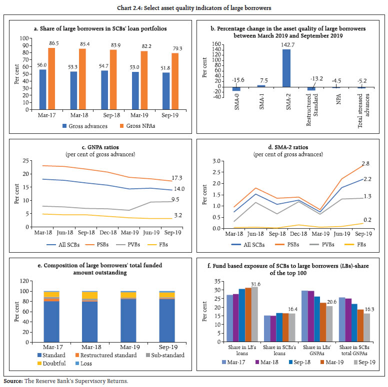
Box 2.1: Dynamics of withdrawn ratings: A snapshot of long-term bank loan rating behaviour Long term bank loan rating is a primary device for credit screening for banks. It also has regulatory implications as the capital adequacy of banking intermediaries is directly linked to external long-term ratings of the obligors that they are exposed to. Box 3.3 examines the credit screening mechanism adopted by investors in short-term instruments and finds a significant dispersion in the pricing of assets of equivalent tenor after accounting for all relevant factors with the same short-term ratings. This implies that these investors must be adopting additional credit screening mechanisms apart from obligor rating during credit selection. Similarly, given the inherent incentive on the part of the banks to boost capital adequacy through optimistic external ratings while at the same time adopting additional mechanism(s) to control aggregate credit risks, the issue of movement in external ratings requires additional scrutiny. In this regard, the Securities and Exchange Board of India (SEBI) has noticed instances where credit rating agencies (CRAs) have provided ‘indicative ratings’ to issuers without entering into written agreements with such issuers12. Since such ‘indicative ratings’ are not disclosed by CRAs on their websites, it becomes difficult to identify instances of possible rating shopping. Some instances of possible ‘rating shopping’ can still, however, be ascertained by looking at the dynamics around rating withdrawals where outstanding rating issued by a CRA was withdrawn and a new rating was provided by a different CRA (within 3 months of each other; in more than two-thirds of the cases new ratings were provided before the withdrawal of the old ones) since April 2016. Chart 1 shows the dynamics of movement across rating grades. Clearly, for ratings that are withdrawn, the new ratings assigned are either the same or an improvement over the earlier ratings. Although replacement of withdrawn ratings by better or similar ratings by a different rating agency is visible across all rating grades, such instances are particularly pronounced at BBB and below possibly because the rated universe has a big concentration around these rating grades. There are only nominal cases where withdrawn ratings were better than the assigned ratings. The issue of possible rating shopping behaviour on the part of obligors clearly requires serious attention. This is particularly relevant as some of the rating agencies have a much greater share in ratings assigned compared to their share in ratings withdrawn (Table 1). Yet, given the fact that the universe of rated obligors is around 40,000, the sample where such distortionary movements are seen represents only a small fraction of the rated universe and may not make the external ratings based capital adequacy framework infructuous.
| Table 1: Share of various rating agencies in withdrawn and assigned ratings | | Rating Agency | Ratings Withdrawn | Rating Assigned | Share in Withdrawn Rating | Share in Assigned Ratings | | CRA 1 | 268 | 209 | 30.8% | 24.0% | | CRA 2 | 261 | 189 | 30.0% | 21.7% | | CRA 3 | 194 | 65 | 22.3% | 7.5% | | CRA 4 | 91 | 73 | 10.5% | 8.4% | | CRA 5 | 39 | 175 | 4.5% | 20.1% | | CRA 6 | 14 | 123 | 1.6% | 14.1% | | CRA 7 | 3 | 36 | 0.3% | 4.1% | | Source: Prime Database and rating agencies’ websites. | |
Risks Banking stability indicator 2.13 The banking stability indicator (BSI)13 shows that there was an improvement in the banking sector’s soundness, profitability, efficiency and liquidity in September 2019 as compared to March 2019 (Chart 2.5). Resilience - Stress tests Macro-stress test - credit risk14 2.14 The resilience of the Indian banking system against macroeconomic shocks was tested through macro-stress tests for credit risks. These tests included a baseline and two adverse (medium and severe) macroeconomic risk scenarios (Chart 2.6). The baseline scenario assumed the continuation of the current economic situation in the future.15 The adverse scenarios were derived based on standard deviations in the historical values of each of the macroeconomic variables separately, that is, univariate shocks: up to 1 standard deviation (SD) of the respective variables for medium risk and 1.25 to 2 SD16 for severe risk (10 years historical data). The horizon of the stress tests is one year. 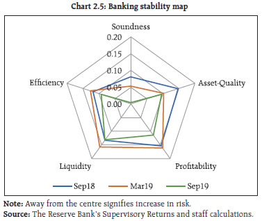 2.15 The stress tests indicate that under the baseline scenario, the GNPA ratios of all SCBs may increase to 9.9 per cent by September 2020 (Chart 2.7) due to change in macroeconomic scenario, marginal increase in slippages and the denominator effect of declining credit growth. Among the bank groups, under the baseline scenario, PSBs’ GNPA ratios may increase to 13.2 per cent by September 2020 from 12.7 per cent in September 2019 whereas for PVBs it may increase to 4.2 per cent from 3.9 per cent; and for FBs it may increase to 3.1 per cent from 2.9 per cent in September 2019. 2.16 Under the assumed baseline macro scenario, CRAR for a system of 53 banks is projected to come down to 14.1 per cent by September 2020 from 14.9 per cent in September 2019. Further deterioration of CRAR is projected under the stress scenarios (Chart 2.8a). 2.17 Three SCBs may have CRAR below the minimum regulatory level of 9 per cent by September 2020 without considering any further planned recapitalisation. However, if macroeconomic conditions deteriorate, five SCBs may record CRAR below 9 per cent under a severe stress scenario (Chart 2.8b).
2.18 Under the baseline scenario, the common equity tier-I (CET-I) capital ratio may decline from 11.9 per cent to 11.3 per cent in September 2020. Two SCBs may have a CET-I capital ratio below the minimum regulatory required level of 5.5 per cent by September 2020. Under a severe stress scenario, the system level CET I capital ratio may decline to 10.1 per cent by September 2020. Two SCBs may have a CET 1 ratio below 5.5 per cent by September 2020 (Chart 2.9). Sensitivity analysis: Bank level18 2.19 A number of single-factor sensitivity stress tests19, based on September 2019 data, were carried out on SCBs to assess their vulnerabilities and resilience under various scenarios20. Their resilience with respect to credit, interest rate and liquidity risks was studied through a top-down21 sensitivity analysis. Credit risk 2.20 Under a severe shock of 2 SD22, that is, if the GNPA ratio of 52 select SCBs moves up to 15.6 per cent from 9.4 per cent, the system-level CRAR will decline from 14.9 per cent to 11.2 per cent and Tier-I CRAR will decline from 12.8 per cent to 9.2 per cent. The impairment in capital at the system level could thus be about 27.1 per cent. The results of the reverse stress test show that it requires a shock of 3.52 SD to bring down the system-level CRAR to 9 per cent. The bank-level stress test results show that 18 banks23 having a share of 36.7 per cent of SCBs’ total assets might fail to maintain the required CRAR under a shock of a 2 SD increase in GNPA ratio (Chart 2.10). PSBs were found to be severely impacted with the CRAR of 16 of the 19 PSBs likely to go down below 9 per cent in case of such a shock. 2.21 Distribution of CRAR of select SCBs shows that under a 2 SD shock on the GNPA ratio, CRAR will come down below 7 per cent for as many as 12 banks, mostly PSBs (Chart 2.11). PVBs and FBs would experience a lesser shift in CRAR under a 2 SD shock while PSBs dominate the right half of the distribution (Chart 2.12).
Credit concentration risk 2.22 Stress tests on banks’ credit concentration, considering top individual borrowers according to their stressed advances, showed that in the extreme scenario of the top three individual borrowers’ failure24, the impact is significant for three banks. These banks account for 3.8 per cent of the total assets of SCBs. The impact on CRAR at the system level under the assumed scenarios of failure of the top 1, 2 and 3 stressed borrowers from each of the banks will be 47, 74 and 96 basis points (Chart 2.13). 2.23 Stress tests on banks’ credit concentration, considering top individual borrowers according to their exposures, showed that in the extreme scenario of the top three individual borrowers’ default25, the impact is significant for only two banks (Chart 2.14). The impact on CRAR at the system level under the assumed scenario of default by all the top three individual borrowers will be 130 basis points.
2.24 Stress tests using different scenarios, based on information about the top group borrowers in the banks’ credit exposure concentration, reveal that the losses could be around 6.2 per cent and 11.3 per cent of the capital at the system level under the assumed scenarios of default by the top group borrower and by the top two group borrowers, respectively. Two banks will not be able to maintain their CRAR level at 9 per cent if top 3 group borrowers default (Table 2.2). | Table 2.2: Credit concentration risk: Group borrowers – exposure | | Shocks | System Level* | Bank Level | | CRAR | Core CRAR | GNPA Ratio | Losses as % of Capital | Impacted Banks (CRAR < 9%) | | Baseline (Before Shock) | 14.9 | 12.8 | 9.4 | --- | No. of Banks | Share in Total Assets of SCBs (in %) | | Shock 1 | The top group borrower defaults | 14.0 | 11.9 | 13.0 | 6.2 | 1 | 0.2 | | Shock 2 | The top 2 group borrowers default | 13.3 | 11.2 | 15.9 | 11.3 | 1 | 0.2 | | Shock 3 | The top 3 group borrowers default | 12.8 | 10.6 | 18.3 | 15.4 | 2 | 2.2 | Note : * : For a system of select 52 SCBs.
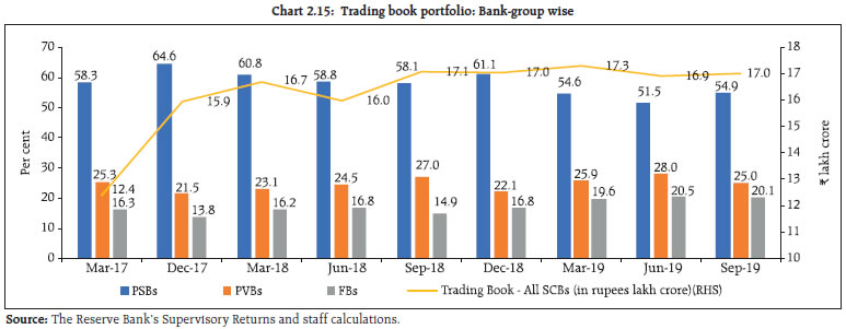
Source: The Reserve Bank’s Supervisory Returns and staff calculations. | Sectoral credit risks 2.25 A sensitivity analysis was done to assess bank-wise vulnerability due to their exposures to certain sub-sectors. Subsector-wise shocks based on respective historical standard deviation (SD) of GNPA ratios were considered to assess the credit risk due to the banks’ exposure to vulnerable subsectors. With a 1 SD shock on the GNPA ratios of some subsectors, the corresponding increase in the GNPAs of 52 banks in different sub-sectors is shown in Table 2.3. 2.26 The resulting losses due to increased provisioning and reduced income were taken into account to calculate a bank’s stressed CRAR and RWAs. The results show that the ‘Infrastructure – Energy’ segment may lead to a decline of 21 bps in the system’s CRAR under a 2 SD shock whereas the ‘Basic Metals and Metal Products’ sector’s exposure may lead to 19 bps decline in the system’s CRAR under a similar shock (Table 2.3). Interest rate risks 2.27 The market value of the portfolio subject to fair value for a sample of 52 SCBs accounting for more than 98 per cent of the total assets of the banking system stood at about ₹17 lakh crore as at end-September 2019 (Chart 2.15). About 91 per cent of the investments subjected to fair value were classified as available for sale (AFS). | Table 2.3: Decline in system level CRAR (bps) (in descending order) | | | 1 SD | 2SD | | Infrastructure - Energy (41 %) | 10 | 21 | | Basic Metal and Metal Products (46%) | 11 | 19 | | Infrastructure - Transport (27%) | 3 | 7 | | All Engineering (37%) | 4 | 6 | | Textiles (23%) | 2 | 4 | | Construction (32%) | 2 | 4 | | Food Processing (23%) | 2 | 3 | | Vehicles, Vehicle Parts and Transport Equipments (43%) | 2 | 3 | | P. Gems and Jewellery (27%) | 1 | 2 | | Mining and Quarrying (31%) | 1 | 1 | Note : * : For a system of select 52 SCBs.
Note: Numbers in parenthesis represent the growth in GNPAs due to 1 SD shock to the Subsector's GNPA ratio.
Source: The Reserve Bank’s Supervisory Returns and staff calculations. |
 2.28 There was an increase in PV0126 of the AFS portfolios of PSBs and FBs compared to the June 2019 values, while that of PVBs showed a marginal decrease. In terms of PV01 curve positioning, the tenor wise distribution of PV01 in PSBs indicates a continuing bias in favour of 5-10 year tenor while in PVBs and FBs the 1-5 year tenor appears to be dominant. A sharp reduction in the corporate tax rate and consequent concerns on borrowing size led to market reaction in the immediate aftermath. However, banks, notably PSBs, are carrying significant interest rate positions in their AFS book, specifically in greater than 5 year tenors (Table 2.4). A somewhat robust deposit growth vis-à-vis a relatively lukewarm credit growth leaves a lot of liquidity chasing interest rate risks. 2.29 With regard to the held for trading (HFT) portfolio size, PVBs and FBs continued to have significant interest rate exposures therein relative to their AFS books, with an increasing trend. The PV01 tenor wise distribution of PVBs and FBs shows dominant exposure in the 1 to 5-year tenor, similar to their AFS positioning (Table 2.5). 2.30 For investments under available for sale (AFS) and held for trading (HFT) categories (direct impact), a parallel upward shift of 2.5 percentage points in the yield curve will lower CRAR by about 81 basis points at the system level (Table 2.6). The total loss of capital at the system level is estimated to be about 6.3 per cent. Table 2.4: Tenor-wise PV01 distribution of the AFS portfolio (in per cent)
(values in brackets are June 2019 figures) | | | Total (in ₹ crore) | < 1 year | 1-5 year | 5-10 year | > 10 years | | PSBs | 247.9 | 4.3 | 26.6 | 47.3 | 21.8 | | | (231.4) | (5.5) | (30.8) | (44.0) | (19.8) | | PVBs | 50.3 | 17.9 | 50.8 | 24.3 | 7.5 | | | (51.2) | (22.7) | (48.8) | (24.7) | (3.7) | | FBs | 37.3 | 9.4 | 66.7 | 13.5 | 10.4 | | | (32.5) | (15.3) | (64.2) | (17.3) | (3.2) | | Source: The Reserve Bank’s Supervisory Returns and staff calculations. |
Table 2.5: Tenor-wise PV01 distribution of the HFT portfolio (in per cent)
(values in the brackets are June 2019 figures) | | | Total (in ₹ crore) | < 1 year | 1-5 year | 5-10 year | > 10 years | | PSBs | 2.1 | 1.9 | 22.8 | 59.9 | 15.3 | | | (1.2) | (5.2) | (8.3) | (84.2) | (2.2) | | PVBs | 14.8 | 7.4 | 50.7 | 31.0 | 21.4 | | | (12.0) | (10.5) | (54.2) | (41.7) | (1.8) | | FBs | 16.3 | 5.4 | 37.9 | 32.8 | 23.9 | | | (14.4) | (12.3) | (47.5) | (33.7) | (6.6) | | Source: The Reserve Bank’s Supervisory Returns and staff calculations. |
Table 2.6: Interest rate risk – bank groups – shocks and impact
(under a shock of 250 basis points parallel upward shift of the INR yield curve) | | | Public Sector Banks | Private Sector Banks | Foreign Banks | All SCBs | | AFS | HFT | AFS | HFT | AFS | HFT | AFS | HFT | | Modified Duration | 2.7 | 3.0 | 1.4 | 1.9 | 1.4 | 2.4 | 2.2 | 2.2 | | Reduction in CRAR (bps) | 101 | 39 | 132 | 81 | | Source: The Reserve Bank’s Supervisory Returns and staff calculations. | Equity price risk 2.31 Under the equity price risk, the impact of a shock of a fall in equity prices on bank capital and profits was examined. The system-wide CRAR will decline by 56 basis points from the baseline under a stressful 55 per cent drop in equity prices (Chart 2.16). The impact of a drop in equity prices is limited for the overall system because considering the regulatory limits prescribed for banks’ exposures to capital markets they typically have a low proportion of capital market exposures on their balance sheets. Liquidity risks: Impact of deposit run-offs on liquid stocks 2.32 The liquidity risk analysis captures the impact of deposit run-offs and increased demand for the unutilised portions of credit lines which were sanctioned/committed/guaranteed. Banks in general may be in a position to withstand liquidity shocks with their high-quality liquid assets (HQLAs)27. In assumed scenarios, there will be increased withdrawals of un-insured deposits28 and simultaneously there will also be increased demand for credit resulting in the withdrawal of the unutilised portions of sanctioned working capital limits and utilisation of credit commitments and guarantees extended by banks to their customers. 2.33 Using their HQLAs required for meeting day-to-day liquidity requirements, 49 of the 52 banks in the sample will remain resilient in a scenario of assumed sudden and unexpected withdrawals of around 10 per cent of deposits along with the utilisation of 75 per cent of their committed credit lines (Chart 2.17).
Stress testing the derivatives portfolio of banks: Bottom-up stress tests 2.34 A series of bottom-up stress tests (sensitivity analyses) on derivative portfolios were conducted for select sample banks29 with the reference date as on September 30, 2019. The banks in the sample reported the results of four separate shocks on interest and foreign exchange rates. The shocks on interest rates ranged from 100 to 250 basis points, while 20 per cent appreciation/depreciation shocks were assumed for foreign exchange rates. The stress tests were carried out for individual shocks on a stand-alone basis. 2.35 Chart 2.18 plots the mark-to-market (MTM) impact as a proportion of CET I capital and as can be seen in the chart, the impact of the sharp moves was mostly muted in individual banks, particularly PSBs and PVBs. Interestingly, in the context of an increase in external commercial borrowings during the current financial year such muted reactions in stress tests (including forex shocks) can only imply that either the corporates have remained unhedged or the forex risks have been transferred out of the banking system to other intermediaries more willing to assume them. As indicated in paragraph 2.42 in the June 2019 edition of FSR there is a need for a thorough assessment of corporates’ hedging profiles as given in the disclosures and possible adoption of macroprudential measures adopted by other jurisdictions towards balance sheet risks in corporate books. 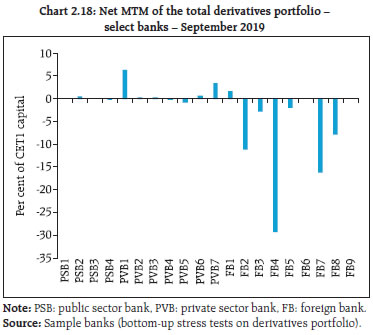
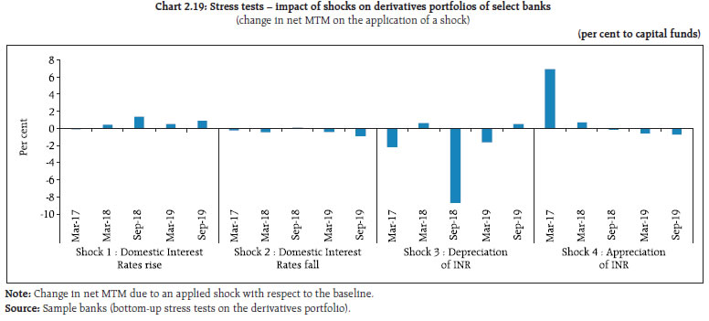 2.36 The stress test’s results showed that the average net impact of interest rate shocks on the sample banks was negligible. The results of the scenario involving appreciation of INR show the effect of shock continuing to normalise in September 2019 from the previous spike (Chart 2.19). Section II Scheduled urban cooperative banks Performance 2.37 The performance of scheduled urban cooperative banks (SUCBs) deteriorated significantly between March and September 2019. At the system level,30 the CRAR of SUCBs declined from 13.5 per cent in March 2019 to 9.8 per cent in September 2019. GNPAs of SUCBs as a percentage of gross advances increased from 6.4 per cent to 10.5 per cent and their provision coverage ratio31 declined from 61.1 per cent to 40.9 per cent during the same period. Further, SUCBs’ RoA turned negative in September 2019 (-3.6 per cent) from 0.7 per cent in March 2019, whereas their liquidity ratios32 marginally increased from 33.5 per cent to 33.9 per cent during the same period. Resilience - stress tests Credit risks 2.38 The impact of credit risk shocks on the SUCBs’ CRAR was observed under 4 different scenarios.33 34 The results show that (i) Under a 1 SD shock to GNPAs classified as loss assets, 10 additional SUCBs failed to achieve the minimum CRAR requirement. The system level CRAR may come down to 7.4 per cent after the shock. (ii) Under a 2 SD shock to GNPAs classified as sub-standard assets, one additional SUCB failed to achieve a 9 per cent CRAR. (iii) Under a 2 SD shock to GNPAs classified as loss advances, 23 more SUCBs failed to maintain the minimum CRAR requirement and the system level CRAR declined significantly to 3.5 per cent. Liquidity risks 2.39 A stress test on liquidity risks was carried out using two different scenarios: i) a 50 per cent, and ii) a 100 per cent increase in cash outflows in the 1-to-28 day time bucket. It was assumed that there was no change in cash inflows under both the scenarios. The stress test’s results show that 24 banks under the first scenario and 39 banks under the second scenario may face liquidity stress.35 Section III Non-banking financial companies 2.40 There were 9,642 NBFCs registered with the Reserve Bank as on September 30, 2019, of which 82 were deposit-accepting (NBFCs-D) and 274 were systemically important non-deposit accepting NBFCs (NBFCs-ND-SI). NBFCs operate through a network of 28,878 branches spread across the country. NBFCs-D and NBFCs-ND-SI are subject to stricter prudential regulations such as capital adequacy requirements and provisioning norms along with reporting requirements.36 Performance Asset quality and capital adequacy 2.41 NBFCs witnessed stress in their asset quality during H1:2019-20. The gross NPA ratio of the NBFC sector increased from 6.1 per cent as at end-March 2019 to 6.3 per cent as at end-September 2019. The net NPA ratio, however, remained steady at 3.4 per cent between end-March 2019 and end-September 2019. As at end-September 2019, the CRAR of the NBFC sector stood at 19.5 per cent, lower than 20 per cent as at end-March 2019 (Table 2.7). | Table 2.7: NBFCs’ asset quality and CRAR37 | | | GNPA Ratio | NNPA Ratio | CRAR | | Mar-15 | 4.1 | 2.5 | 26.2 | | Mar-16 | 4.5 | 2.5 | 24.3 | | Mar-17 | 6.1 | 4.4 | 22.1 | | Mar-18 | 5.3 | 3.3 | 22.1 | | Mar-19 | 6.1 | 3.4 | 20.0 | | Sep-19 | 6.3 | 3.4 | 19.5 | NBFCs’ vulnerabilities – ALM issues 2.42 While the importance of NBFCs in credit intermediation is growing, the IL&FS episode brought the focus on the asset liability mismatches of NBFCs, which poses risks to the NBFC sector as well as the financial system as a whole. To address such concerns, the Reserve Bank introduced the liquidity coverage ratio (LCR) requirement for all deposit-taking NBFCs and non-deposit taking NBFCs with an asset size of ₹5,000 crore and above (constituting 87 per cent of the total assets of the NBFC sector). The new regulation mandates NBFCs to maintain a minimum level of high-quality liquid assets to cover expected net cash outflows in a stressed scenario. NBFCs are required to reach a LCR of 100 per cent over a period of 4 years commencing from December 2020. Resilience - stress tests38 System level 2.43 Stress tests for the NBFC sector’s credit risk as a whole for the year ended September 2019 were carried out under three scenarios: Increase in GNPA by (i) a 0.5 SD, (ii) 1 SD and (iii) 3 SD. The results show that in the first scenario, the sector’s CRAR declined from 19.5 per cent to 18.9 per cent. In the second scenario, it declined to 18.1 per cent and in the third scenario it came down to 15.1 per cent. Individual NBFCs 2.44 The stress test’s results for individual NBFCs show that under the first two scenarios (increase in GNPA by 0.5 SD and 1 SD), around 8.6 per cent of the companies will not be able to comply with the minimum regulatory capital requirements of 15 per cent. Around 14.2 per cent of the companies will not be able to comply with the minimum regulatory CRAR norms under the third scenario, that is, an increase in GNPA by 3 SD. Section IV A. The real estate sector 2.45 The real estate sector has recently been in focus owing to developments both in the NBFC and banking sectors brought about by their real estate exposures. To get a ringside view of the financial strength of some of the major participants in the sector, the performance of 310 real estate companies (REs), as reflected in the books of the financial intermediaries having exposures to these entities since June 2016 was tracked. 2.46 Table 2.8 looks at the evolution of various financial intermediaries for the REs since June 2016. As can be seen in the table, while the aggregate exposure to REs approximately doubled, the aggregate share of HFCs and PVBs increased while PSBs’ aggregate share reduced sharply. This might, however, understate the exposure of PSBs to the sector given their exposure to a few NBFCs well entrenched in the real estate sector. Another important aspect that emerges from Table 2.8 is that the flow of funds to the sector has continued notwithstanding a general slowdown in credit growth documented earlier. Since September 2018 when the IL&FS induced risk aversion was noted, all categories of financial intermediaries have increased their exposures to REs, the sharpest being that of HFCs. Table 2.8: Relative share of exposures39 of various financial intermediaries
(For the sample of 310 real estate companies) | | (per cent) | | | HFCs | NBFCs | PSBs | PVBs | FBs | Others | Total (₹ crore) | | Jun-16 | 12.17 | 6.42 | 48.57 | 23.62 | 8.46 | 0.76 | 1,04,932 | | Jun-17 | 18.14 | 9.58 | 40.66 | 26.01 | 5.20 | 0.41 | 1,21,640 | | Jun-18 | 20.56 | 10.77 | 29.77 | 27.98 | 10.50 | 0.43 | 1,66,286 | | Jun-19 | 23.81 | 9.52 | 24.34 | 30.41 | 11.62 | 0.30 | 2,01,171 | | Source: TransUnion CIBIL. | 2.47 Table 2.9 looks at the evolution of impairment levels in this portfolio of 310 REs. The impairment numbers are cumulative in the sense that a company deemed impaired in the earlier quarter continues to be included as impaired till it comes out of the same. The impairment is based on 90 days past due (dpd). As can be seen in Table 2.9, the aggregate impaired exposures continued to rise steadily over the period of observation, with delinquency levels of all financial intermediaries higher as on June 2019 compared to their June 2018 levels. Given the structure of the sample this should be indicative of the evolution of general industry-wide portfolio health of REs rather than health of the real estate exposure in specific financial intermediaries. 2.48 To evaluate the effect of legacy impairment on aggregate numbers, Table 2.10 examines the movement in the 180+dpd/loss segment of the portfolios across financial intermediaries. Clearly the legacy load is fairly sizeable with regard to NBFCs/ PSBs while PVBs and HFCs’ portfolios are subject to recent slippages. 2.49 To conclude, the analysis of 310 real estate related obligors gives evidence of increased stress although the aggregate exposure to the sample firms continued to increase, implying availability of credit. However, the aggregate numbers for HFCs/ NBFCs / PVBs, while increasing, are relatively small in absolute amounts. PSBs’ exposure, particularly with regard to impairment is fairly large. However, this has to be seen in the context of their aggregate real estate portfolio performance. B. Consumer credit and developments in the non-banking space – a follow up 2.50 The June 2019 issue of the Financial Stability Report did a thematic exploration of consumer credit. The exploration noted an adverse selection bias, that is, consumer credit portfolio of NBFCs and HFCs has relatively higher delinquency rates as compared to SCBs. Given the continuing churn in the non-banking financial space as evidenced through the weighted inter-quartile differences in commercial paper (CP) rates outlined in Chapter 1, the portfolio health of these two sectors as evidenced in the delinquency numbers in the last two quarters is now outlined. Table 2.9: Evolution of impairment levels across financial intermediaries
(For the sample of 310 real estate companies) | | (per cent) | | | HFCs | NBFCs | PSBs | PVBs | FBs | Total | | Jun-16 | 0.00 | 0.11 | 7.06 | 1.76 | 0.00 | 3.90 | | Jun-17 | 0.00 | 0.12 | 9.67 | 1.66 | 0.00 | 4.38 | | Jun-18 | 0.03 | 2.00 | 15.00 | 2.64 | 2.51 | 5.74 | | Jun-19 | 2.09 | 2.31 | 18.71 | 5.41 | 2.83 | 7.33 | | Source: TransUnion CIBIL. |
Table 2.10: Evolution of 180+ dpd / loss assets across financial intermediaries
(For the sample of 310 real estate companies) | | (per cent) | | | HFCs | NBFCs | PSBs | PVBs | FBs | Total | | Jun-16 | 0.00 | 0.01 | 3.82 | 0.56 | 0.00 | 2.00 | | Jun-17 | 0.00 | 0.00 | 7.07 | 1.66 | 0.00 | 3.31 | | Jun-18 | 0.03 | 0.05 | 13.17 | 2.42 | 0.00 | 4.64 | | Jun-19 | 0.00 | 1.69 | 14.61 | 1.41 | 2.17 | 4.42 | | Source: TransUnion CIBIL. | 2.51 Table 2.11 gives the relative delinquency in auto loans which appears to be stabilising across financial intermediaries with the exception of NBFCs. The stabilising delinquency in PSBs' and PVBs' portfolios is particularly impressive in the context of slowing consumer credit growth in auto loans in Q1:2019-20 (Industry Insights Report, Second Quarter, 2019-TransUnion CIBIL). The trend is similar in ‘home loans’ where the HFCs’ portfolio shows a disproportionate increase, possibly owing to a relative slowdown in the growth in the segment (NBFC portfolio delinquency in this segment is higher but NBFCs’ share of the home loan portfolio is small and hence may not be reflective of the health of the sector) (Table 2.12). A relative slowdown is also seen in home loan origination volumes reflecting the generally soft activity in the real estate sector. 2.52 Loans against property (LAP) saw the most significant increase in delinquencies over the last year among major consumer credit products (Industry Insights Report, Second Quarter, 2019- TransUnion CIBIL) with the NBFC and PSB sectors being the worst affected (Table 2.13). As a possible precautionary measure, LAP origination volumes by PSBs and NBFCs showed a sharp decline during the June 2019 quarter as has been noted by TransUnion CIBIL. They also noted a shift by PVBs towards higher risk tiers in this segment. In sharp contrast, the personal loan segment continued its healthy growth in Q1:2019-20 led by NBFCs although NBFCs still lead the delinquency trend (Table 2.14). | Table 2.11: Relative delinquency in auto loans | | (per cent) | | | Mar-17 | Mar-18 | Mar-19 | Jun-19 | | PSBs | 3.50 | 2.80 | 2.60 | 2.60 | | PVBs | 1.70 | 1.60 | 0.90 | 0.90 | | NBFCs | 5.80 | 4.40 | 4.30 | 4.70 | | Industry | 3.70 | 2.80 | 2.50 | 2.70 | | Source: TransUnion CIBIL. |
| Table 2.12: Relative delinquency in home loans | | (per cent) | | | Mar-17 | Mar-18 | Mar-19 | Jun-19 | | PSBs | 2.10 | 1.90 | 2.00 | 1.80 | | PVBs | 0.60 | 0.70 | 0.70 | 0.70 | | NBFCs | 3.80 | 2.90 | 3.10 | 3.20 | | HFCs | 1.00 | 1.30 | 1.50 | 1.80 | | Industry | 1.50 | 1.50 | 1.60 | 1.70 | | Source: TransUnion CIBIL. |
| Table 2.13: Relative delinquency in loans against property | | (per cent) | | | Mar-17 | Mar-18 | Mar-19 | Jun-19 | | PSBs | 4.50 | 5.10 | 5.70 | 6.50 | | PVBs | 1.00 | 1.10 | 1.50 | 1.60 | | NBFCs | 3.40 | 4.10 | 4.80 | 5.20 | | HFCs | 1.20 | 1.70 | 2.10 | 2.60 | | Industry | 2.30 | 2.60 | 3.10 | 3.50 | | Source: TransUnion CIBIL. |
| Table 2.14: Relative delinquency in personal loans | | (per cent) | | | Mar-17 | Mar-18 | Mar-19 | Jun-19 | | PSBs | 0.70 | 0.40 | 0.60 | 0.40 | | PVBs | 0.40 | 0.50 | 0.50 | 0.50 | | NBFCs | 0.60 | 0.80 | 1.00 | 1.00 | | Industry | 0.60 | 0.60 | 0.60 | 0.60 | | Source: TransUnion CIBIL. | 2.53 In conclusion, emerging trends in consumer credit continue to show a challenging environment for NBFCs. This issue is of specific relevance since a recent industry report on the MSME40 sector (MSME Pulse, October, 2019-TransUnion CIBIL) also noted a sharp rise in delinquency as also slackening of credit growth in the commercial credit segment for NBFCs. Section V Network of the financial system41 2.54 A financial system can be visualised as a network if the financial institutions are considered as nodes and the bilateral exposures between them as links joining these nodes. Financial institutions establish links with other financial institutions for efficiency gains and risk diversification, but these same links also lead to risk transmission in a financial crisis. 2.55 The total outstanding bilateral exposures42 among the entities in the financial system amounted to ₹35 lakh crore as at end-September 2019. The y-o-y growth in bilateral exposures during this period declined to 7.7 per cent from double digit growth rates witnessed in the past (Chart 2.20a). 2.56 SCBs continued to be the dominant players accounting for 44.2 per cent of the financial system’s bilateral exposures as at end-September 2019 though their share declined in the last two quarters (Chart 2.20b). 2.57 Share of asset management companies – mutual funds (AMC-MFs), NBFCs and HFCs stood at 14.3, 13.4 and 8.9 per cent, respectively as at end-September 2019. The share of NBFCs in the financial system’s bilateral exposures witnessed a gradually increasing trend (Chart 2.20b). 2.58 The share of insurance companies in total bilateral exposures which fluctuated in the narrow band of 8.3-8.7 per cent over the last few quarters, increased to 9.2 per cent as at end-September 2019. All India financial institutions (AIFIs) had a share in the range of 7.3-8.8 per cent in the last two years. The share of pension funds (PFs) was relatively low in the range of 0.8-1.3 per cent, though there was a gradually increasing trend over the quarters. SUCBs had a negligible share of about 0.3 per cent in bilateral exposures. It is, however, to be noted that due to a small share in bilateral exposure, direct impact of contagion may be minimal but confidence channels can still carry the contagion. 2.59 In terms of inter-sectoral43 exposures, AMC-MFs followed by the insurance companies were the major fund providers to the system, while NBFCs followed by HFCs and SCBs were the major receivers of funds. Within the SCBs, PVBs had a net payable position vis-à-vis the entire financial sector, whereas PSBs had a net receivable position (Chart 2.21). 2.60 The net receivables of AMC-MFs and insurance companies from the financial sector, grew at 12.5 per cent (y-o-y) and 17 per cent (y-o-y), respectively, as at end-September 2019. Over the same period, PSBs registered a decline in net receivables by 12.4 per cent. On the other hand, the annual growth in PVBs’ net payables to the financial system was 20.8 per cent. For NBFCs and HFCs, net payables grew at 10.6 per cent and 5.5 per cent, respectively, owing primarily to increased borrowings by public sector NBFCs and large HFCs (Chart 2.22).
The inter-bank market 2.61 The size of the inter-bank market (both fund-based44 and non-fund-based45), as a proportion of total assets of the banking system has consistently declined over the last few years. Fund based inter-bank exposures as a share of total assets of the banking system moderated to 3.2 per cent as at end-September 2019 from 3.8 per cent as at end-September 2018 (Chart 2.23). 2.62 PSBs continued to dominate the inter-bank market with a share of 54.1 per cent (as compared to a share of 60.3 per cent in total bank assets) followed by PVBs at 32.3 per cent (share of 33.2 per cent in total bank assets) and FBs at 13.6 per cent (share of 6.5 per cent in total bank assets) as at end-September 2019 (Chart 2.24). 2.63 As at end-September 2019, 72 per cent of the fund-based inter-bank market was short-term (ST) in nature in which the highest share was of ST deposits followed by ST loans and call money (Call). The compositon of long-term (LT) fund based exposure shows that LT loans has the highest share followed by LT deposits (Chart 2.25).
Inter-bank market: Network structure and connectivity 2.64 The inter-bank market usually has a core-periphery structure. The network structure46 of the banking system47 at end-September 2019 shows that there were 5 banks in the inner-most core and 8 banks in the mid core. 2.65 During the last 5 years, the number of banks in the inner-most core ranged between two and five. These were usually the biggest PSBs or PVBs. Most foreign banks and almost all ‘old’ private banks were usually in the outermost periphery making them the least connected banks in the financial system. The remaining PSBs and PVBs along with a few major FBs made up the mid and outer-cores (Chart 2.26). 2.66 The degree of interconnectedness in the banking system (SCBs), as measured by the connectivity ratio48, has been decreasing slowly over the last few years. This is in line with a shrinking inter-bank market as mentioned earlier. The cluster coefficient49, which depicts local interconnectedness (the tendency to cluster), has not varied much in the last 5 years. This indicates that clustering/grouping within the banking network has not changed much over time (Chart 2.27). Exposure of AMC-MFs 2.67 AMC-MFs were the largest net providers of funds to the financial system. Their gross receivables were around ₹ 9,40,285 crore (around 37.8 per cent of their average assets under management (AUM) as on September 2019), and their gross payables were around ₹ 57,355 crore as at end-September 2019. 2.68 The top-3 recipients of their funds were SCBs followed by NBFCs and HFCs. AMC-MFs' receivables from SCBs which had increased in FY 2018-19 moderated in H1:2019-20. AMC-MFs’ receivables from NBFCs have exhibited a gradually decreasing trend since June 2018, while receivables from HFCs which had been on a declining trend since September 2018 registered an increase during Q2:2019-20 (Chart 2.28a). 2.69 An instrument-wise break-up of AMC-MFs’ receivables shows that AMC-MFs have reduced their CP exposures to NBFCs and HFCs. The share of certificates of deposit (CD) funding which sharply expanded in the second half of 2018-19, witnessed a fall after March 2019 (Chart 2.28b).
Exposure of insurance companies 2.70 Insurance companies had gross receivables of ₹5,98,875 crore and gross payables of around ₹25,980 crore, making them the second largest net providers of funds to the financial system as at end-September 2019. 2.71 As in the case of AMC-MFs, a breakup of insurance companies’ gross receivables indicates that the top 3 recipients of their funds were SCBs followed by NBFCs and HFCs. Long term (LT) debt and equity accounted for almost all the receivables of insurance companies, with limited exposure to short-term instruments. While the share of LT debt has been falling gradually, the share of equity has been increasing over the last 2 years (Charts 2.29a and b). Exposure to NBFCs 2.72 NBFCs were the largest net borrowers of funds from the financial system with gross payables of around ₹8,29,468 crore and gross receivables of around ₹66,635 crore as at end-September 2019. A breakup of gross payables indicates that 48.4 per cent of the funds were obtained from SCBs followed by 26 per cent from AMC-MFs and 21.3 per cent from insurance companies. The share of SCBs which had increased during FY 2018-19 registered a moderate decline in H1:2019-20. Share of AMC-MFs has been on a declining trend since the last few quarters (Chart 2.30 a). 2.73 The choice of instruments in the NBFC funding mix clearly shows the increasing role of LT loans (provided by SCBs and AIFIs) and a declining share of CPs (primarily subscribed to by AMC-MFs and to a lesser extent by SCBs) and LT debt (held by insurance companies and AMC-MFs) (Chart 2.30b). Exposure to housing finance companies 2.74 HFCs were the second largest borrowers of funds from the financial system with gross payables of around ₹5,90,039 crore and gross receivables of only ₹33,110 crore as at end-September 2019. HFCs’ borrowing pattern was quite similar to that of NBFCs except that AIFIs also played a significant role in providing funds to HFCs. Share of AMC-MFs in providing funding to HFCs came down sharply in the last year, only registering a marginal increase in Q2:2019-20. In contrast, the relative share of SCBs showed an upward trend, but dipped in September 2019 (Chart 2.31a). 2.75 As in the case of NBFCs, LT debt, LT loans and CPs were the top 3 instruments through which HFCs raised funds from the financial systems though their funding mix has been in a flux in the last six quarters. Reliance on CPs (subscribed to by AMC-MFs and to a lesser extent by SCBs) which had increased considerably in H1:2018-19 saw a sharp fall thereafter. This was compensated for by the increasing share of LT loans (from banks and AIFIs) and LT debt (Chart 2.31b). The CP and CD markets50 2.76 Among all the short-term instruments through which financial institutions raise funds from each other, CP and CD are the most important. In the CP market, AMC-MFs are the biggest investors and HFCs, NBFCs and AIFIs are the biggest issuers. In the CD market, AMC-MFs are the biggest investors and PVBs are by far the biggest issuers followed by PSBs. The size of the CD market which shot up during the second-half of 2018-19, witnessed a sharp fall after March 2019. The size of the CP market has also shrunk considerably in the last one year (Chart 2.32).
Contagion analysis51 Joint solvency52-liquidity53 contagion losses to the banking system due to idiosyncratic bank failure 2.77 Contagion analysis is a network technique used for estimating the systemic importance of different banks. Failure of a bank which is systemically more important leads to greater solvency and liquidity losses to the banking system. Solvency and liquidity losses, in turn, depend on the initial capital and liquidity position of the banks along with the number, nature (whether it is a lender or a borrower) and magnitude of the interconnections that the failing bank has with the rest of the banking system. 2.78 In this analysis, banks are triggered (assumed to have failed) one at a time and their impact on the banking system is seen in terms of the number of subsequent bank failures that take place and the amount of solvency and liquidity losses that are incurred (Chart 2.33). 2.79 Contagion analysis of the banking network54 indicates that if the bank with the maximum capacity to cause contagion losses fails (that is, Bank 1), it will lead to a solvency loss of 3.2 per cent of the total Tier-I capital of the banking system and a liquidity loss of 0.3 per cent of the total liquid assets. The losses as at end-September 2019 are lower compared to end-March 2019 (FSR June 2019) due to a better capitalised public sector banking system and a shrinking inter-bank market (Table 2.15). Solvency contagion losses to the banking system due to idiosyncratic NBFC/HFC failure 2.80 As noted earlier, NBFCs and HFCs are the largest and the second largest borrowers of funds from the financial system. A substantial part of this funding comes from banks. Therefore, failure of any NBFC55 or HFC will act as a solvency shock to its lenders. The solvency losses caused by these shocks can further spread by contagion either due to direct linkages among the lenders or due to an information contagion. 2.81 Here, the quantum of solvency contagion losses56 to the banking system caused by the idiosyncratic failure of a NBFC/HFC are assessed. The results are presented in Tables 2.16 and 2.17. Failure of a NBFC with the maximum capacity to cause solvency losses to the banking system (labelled as NBFC 1 in Table 2.16) will cause a loss of 2.5 per cent of the total Tier-I capital of the banking system. Failure of a HFC with the maximum capacity to cause solvency losses to the banking system (labelled as HFC 1 in Table 2.17) will lead to a loss of 4.6 per cent of the total Tier-I capital of the banking system. In either case, that is, NBFC or HFC failure, no additional bank will fail. Table 2.15: Top 5 banks with maximum contagion impact – September 2019
(joint solvency-liquidity contagion) | | Trigger Bank | Solvency losses as a % of Tier-I capital | Liquidity losses as a % of HQLAs | Number of defaulting banks due to solvency | Number of defaulting banks due to liquidity | Total | | Bank 1 | 3.2 | 0.3 | 0 | 0 | 0 | | Bank 2 | 2.7 | 0.1 | 1 | 0 | 1 | | Bank 3 | 2.5 | 0.2 | 1 | 0 | 1 | | Bank 4 | 2.4 | 1.8 | 1 | 3 | 4 | | Bank 5 | 2.3 | 0.8 | 0 | 0 | 0 | Note: Top 5 ‘trigger banks’ were selected on the basis of solvency losses caused to the banking system.
Source: The Reserve Bank’s Supervisory Returns and staff calculations |
| Table 2.16: Top 5 NBFCs with maximum contagion impact - September 2019 | | Trigger | Solvency losses as a % of total Tier-I capital of banks | Number of defaulting banks | | NBFC 1 | 2.5 | 0 | | NBFC 2 | 1.7 | 0 | | NBFC 3 | 1.7 | 0 | | NBFC 4 | 1.5 | 0 | | NBFC 5 | 1.3 | 0 | Note: Top 5 ‘trigger NBFCs’ were selected on the basis of solvency losses caused to the banking system.
Source: The Reserve Bank’s Supervisory Returns and staff calculations. |
| Table 2.17: Top 5 HFCs with maximum contagion impact - September 2019 | | Trigger | Solvency losses as a % of total Tier-I capital of banks | Number of Defaulting banks | | HFC 1 | 4.6 | 0 | | HFC 2 | 2.8 | 0 | | HFC 3 | 2.3 | 0 | | HFC 4 | 2.2 | 0 | | HFC 5 | 1.5 | 0 | Note: Top 5 ‘trigger HFCs’ were selected on the basis of solvency losses caused to the banking system.
Source: The Reserve Bank’s Supervisory Returns and staff calculations | Solvency contagion impact57 after macroeconomic shocks to SCBs 2.82 The contagion impact of a bank’s failure is likely to be magnified if macroeconomic shocks result in distress in the banking system in a situation of a generalised downturn in the economy. Macroeconomic shocks are given to SCBs which lead to some SCBs failing the solvency criterion, which then acts as a trigger causing further solvency losses. The initial impact of macroeconomic shocks on individual banks’ capital was taken from the macro-stress tests, where a baseline and two (medium and severe) adverse scenarios were considered for September 2020.58 2.83 Initial capital losses due to macroeconomic shocks are 5.4, 9.8 and 14.4 per cent of Tier-I capital of the banking system for baseline, medium and severe stress scenarios, respectively. The number of banks failing due to macroeconomic shocks are three for baseline, three for medium and four for severe stress (Chart 2.34). 2.84 The contagion impact overlaid on the outcome of the macro-stress test shows that additional solvency losses due to contagion (on top of the initial loss of capital due to the macro shocks) to the banking system in terms of Tier-I capital are limited to 0.8 per cent for the baseline, 0.8 per cent for medium stress and 1 per cent for severe stress scenarios. Also, the additional number of defaulting banks due to contagion (excluding initial defaulting banks due to the macro shocks) is zero for baseline and medium stress scenarios and 1 for severe stress scenario (Chart 2.34).
|