by
KL Krishna
Bishwanath Goldar
Deb Kusum Das
Suresh Chand Aggarwal
Abdul Azeez Erumban
Pilu Chandra Das The views expressed in this Report are those of the authors and should not be attributed to the Centre for Development Economics as an Institution. © 2022 jointly held by K.L. Krishna, Bishwanath Goldar, Deb Kusum Das, Suresh Chand Aggarwal, Abdul Azeez Erumban and Pilu Chandra Das, the authors of the Report Centre for Development Economics
Delhi School of Economics
University of Delhi
Delhi 110007, India
www.econdse.org |
| Contents | | Foreword | | Preface and Acknowledgements | | Chapter 1: Introduction to India KLEMS Approach | | 1.1 Introduction | | 1.2 Evolution of India KLEMS Research | | 1.3 Global Productivity Research | | 1.4 Productivity research in India | | 1.4.1 Early Research | | 1.4.2 Recent Research | | 1.4.3 Productivity research based on KLEMS database | | 1.5 Report summary and contribution of chapters | | Annexure 1A: List of Industries in India KLEMS Database | | Annexure 1B: The data sources and construction of variables – key points | | Annexure 1C: Publications of the Research Team Based on India KLEMS Database | | Chapter 2: Sources and Methodology: India KLEMS Database | | 2.1 Introduction | | 2.2 Approach to measuring productivity in India KLEMS: The growth accounting methodology | | 2.2.1 The KLEMS production function | | 2.2.2 The decomposition of value added and output growth | | 2.3. Data and Variables: Construction and Approaches | | 2.3.1 Gross Output | | 2.3.2 Gross Value Added | | 2.3.3 Intermediate inputs | | 2.3.4 Labour Input | | 2.3.5 Capital Input | | 2.3.6 Labour Income Share | | 2.4 Data Challenges & Outstanding Issues | | 2.4.1 Gross Output and Intermediate Inputs | | 2.4.2 Labour Input | | 2.4.3 Labour Income Share | | 2.4.4 Capital Input | | 2.4.5 Methodology of TFP Measurement | | 2.5 Summary | | Annexure 2A: Additional Tables | | Chapter 3: Economic Growth in India: An Industry Perspective | | 3.1 Introduction | | 3.2 Changes in the structure of the economy | | 3.3 Aggregate value-added growth and industry and broad sector contributions to aggregate growth | | 3.4 Growth of industry output and intermediate inputs | | 3.5 Summary and Conclusion | | Annexure 3A: Additional Table | | Chapter 4: Employment, Labour Quality and Labour Income Share | | 4.1 Introduction | | 4.2 Profile of the Workforce since 1980-81 | | 4.3 Structure and growth in employment | | 4.3.1 Structure of employment in India during 1980-2017 | | 4.3.2 Growth in employment | | 4.4 Growth in Labour Quality Index | | 4.4.1 Growth in Labour Quality index in Broad sectors | | 4.4.2 Growth in labour quality index for the 27 India KLEMS industries | | 4.5 Growth in Labour Input | | 4.5.1 Growth in Labour Input in Broad sectors | | 4.5.2 Growth in Labour Input for the 27 KLEMS industries | | 4.6 Labour Income Share | | 4.6.1 Trends in labour income share in India | | 4.6.2 The volatility of the labour income share | | 4.6.3 Reallocation of change in the labour income share | | 4.7 Summary and Conclusion | | Annexure 4A: Additional Tables | | Annexure 4B: Trends in employment in the period 2011-2017 – assessing the impact of growth in real wages | | Chapter 5: Investment and Capital Input | | 5.1 Introduction | | 5.2 Composition and Growth of Investment | | 5.2.1 Distribution of Investment across Broad Sectors | | 5.2.2 Growth rate of real investment by broad sectors | | 5.3 Composition and growth rates of capital stock | | 5.3.1 Changing composition of capital stock | | 5.3.2 Growth rates of capital stock | | 5.4 Capital service growth rates | | 5.5 Capital composition effects | | 5.6 Summary and conclusions | | Annexure 5A: Additional Tables | | Chapter 6: Trends and drivers of labour productivity in Indian industries | | 6.1 Introduction | | 6.2: Literature on Labour Productivity | | 6.3. Methodology and Dataset | | 6.3.1 Measurement of labour productivity | | 6.3.2 Sources of Labour productivity growth | | 6.3.3 Decomposition of labour productivity- within and between effects | | 6.3.4 Data and variables | | 6.4: Labour Productivity – Trends and behaviour | | 6.4.1 Labour Productivity growth in the disaggregate industries | | 6.4.2 Changes in the growth rate of labour productivity | | 6.5 Sources of Growth in Labour Productivity and the ‘virtuous’ pattern of growth | | 6.5.1 Sources of Growth in Labour Productivity | | 6.5.2 The virtuous pattern of growth of labour productivity | | 6.6 Labour productivity at the broad sectoral level, reallocation and sectoral decomposition | | 6.6.1 Level of labour productivity in the broad sectors | | 6.6.2 Growth of labour productivity in the broad sectors | | 6.6.3 Labour Productivity: Reallocation and Sectoral Decomposition | | 6.7 A cross-country comparison of labour productivity | | 6.8 Summary and Conclusion | | Annexure 6A: Additional Table | | Chapter 7: Industry origins of Aggregate Growth and Total Factor Productivity | | 7.1 Introduction | | 7.2 Review of Indian Growth and Productivity Literature | | 7.2.1 Studies based on non-India KLEMS datasets | | 7.2.2 Studies based on the India KLEMS datasets | | 7.3 Methodology | | 7.3.1 Production Possibility Frontier (PPF) approach | | 7.3.2 Direct Aggregation across Industries | | 7.3.3 Sectoral Aggregation | | 7.4 Disaggregated Empirical Results, 1980-17 | | 7.4.1 Sources of Industry-level Output Growth | | 7.4.2 Industry Origins of Aggregate Growth and Productivity | | 7.4.3 Industry contributions to growth of aggregate primary inputs | | 7.5 Disaggregated Growth & Productivity Dynamics – Pre & Post Global Financial Crisis | | 7.5.1 Changes in sources of output growth, 2008-17 less 1993-07 | | 7.5.2 Changes in industry contributions to aggregate growth & productivity, 2008-17 less 1993-07 | | 7.5.3 Changes in industry contributions to growth of aggregate primary inputs, 2008-17 less 1993-07 | | 7.6 Sectoral Origins of Growth & Productivity | | 7.7 Summary & Conclusions | | Annexure 7A: Additional Tables | | Chapter 8: Growth, Employment and Labour Productivity in Formal and Informal Manufacturing | | 8.1 Introduction | | 8.2 Formal-Informal Divide and the Role of the Informal Sector | | 8.2.1 Formal-Informal Divide in Employment | | 8.2.2 Informality in India | | 8.3. Dataset and Methodology | | 8.3.1 Data | | 8.3.2 Methodology | | 8.4 Relative Share of the Manufacturing Sector and the Extent of Informality | | 8.4.1 Manufacturing sector | | 8.4.2 Informality in the manufacturing sector of India | | 8.5 Growth in Real GVA, Organized and Unorganized Manufacturing | | 8.6 Growth in Employment, Organized and Unorganized Manufacturing | | 8.7 Labour Productivity in the unorganized and organized sector of the Indian economy | | 8.7.1 Labour productivity – trends and behaviour | | 8.7.2 Informality: Role in stagnant growth and sectoral decomposition | | 8.7.3 Decomposition of aggregate labour productivity growth - the reallocation effect | | 8.8 Summary and Conclusion | | Annexure 8A: Construction of real GVA series for organized and unorganized segments of manufacturing industries | | Annexure 8B: Growth rate in real GVA series in organized and unorganized segments of manufacturing industries, 1981-2017 | | Annexure 8C: Growth in employment in organised and unorganised segments of manufacturing, 1981-2017 | | Chapter 9: Capital Intensity in Industries | | 9.1 Introduction | | 9.2 Trends in capital intensity | | 9.2.1 Capital intensity in the aggregate economy and broad sectors | | 9.2.2 Capital intensity in the 27 KLEMS industries | | 9.3 Growth in Capital Intensity, Labour Productivity and Real Wages | | 9.4 Wage-rental ratio and capital intensity of the Indian economy: Econometric Analysis | | 9.4.1 Relative prices of capital | | 9.4.2 Effect of Wage-rental ratio on and capital intensity – Aggregate Economy | | 9.4.3 Impact of real wage on capital intensity – estimate for manufacturing based on a panel data model | | 9.5 Conclusion | | Chapter 10: Energy Intensity in Manufacturing Industries | | 10.1 Energy intensity | | 10.1.1 Trends in energy intensity in aggregate manufacturing | | 10.1.2 Trends in energy intensity in organised manufacturing | | 10.1.3 Impact of energy prices on energy intensity in organised manufacturing | | 10.2 Determinants Energy Use and Energy Intensity in Organized Manufacturing | | 10.3 Conclusion | | Annexure 10A: Construction of energy use and energy intensity series for manufacturing | | Annexure 10B: Construction of Industry-level energy use and energy-intensity series for organized manufacturing | | Annexure 10C: ARDL Model Estimation for Explaining Energy Intensity of Manufacturing using Time-series Data at the Aggregate Manufacturing Level | | Chapter 11: Growth and Productivity in India’s Services sector | | 11.1 Introduction | | 11.2 Service Sector Liberalization: An Overview | | 11.3 Service Sector Performance: 1980-2017 | | 11.4. Productivity Trends in India’s Service Sector | | 11.5. Conclusions | | Annexure 11A: Policies Relating to Services Sector | | Chapter 12: Growth and Productivity: A China and India comparison | | 12.1 Introduction | | 12.2 Labour Productivity and growth in India and China: The aggregate picture | | 12.3 Aggregations of KLEMS industry growth rates: Methodology and data | | 12.3.1 Methodology | | 12.3.2 CIP/China KLEMS Data | | 12.4 Empirical results | | 12.4.1 Labour productivity and TFP in the broad sectors of the economy | | 12.4.2 Labour productivity and TFP in the select industry groups of the economy | | 12.4.3 The industry pattern of aggregate TFPG | | 12.4.4 Capital deepening and labour productivity growth – a comparative perspective | | 12.5 Conclusion | | Annexure 12A: India KLEMS and China KLEMS, Concordance | | Chapter 13: Summary and Conclusion | | 13.1 The context | | 13.2 Outputs and Inputs | | 13.2.1 Output, value added and intermediate inputs | | 13.2.2 Labour input and labour income share | | 13.2.3 Capital input | | 13.2.3 Capital input | | 13.3 Labour Productivity and Total Factor Productivity | | 13.4 The Performance of Manufacturing – formal-informal divide and energy use | | 13.4.1 Formal-Informal Divide | | 13.4.2 Energy intensity of manufacturing | | 13.5 Capital intensity: A relook at the trends and underlying factors | | 13.6 Services as an engine of Growth | | 13.7 Comparative performance of India and China | | 13.8 India KLEMS: The way forward | | 13.8.1 Intangible investment | | 13.8.2 ICT capital | | 13.8.3 Informal sector | | 13.8.4 Relaxing neoclassical assumptions | | 13.8.5 Productivity implications for welfare | | References |
| Abbreviations | | ASI | - | Annual Survey of Industries | | CSO | - | Central Statistics Office | | EMDE | - | Emerging Market and Developing Economies | | EUS | - | Employment-Unemployment Survey | | GDP | - | Gross Domestic Product | | GFC | - | Global Financial Crisis | | GFCF | - | Gross Fixed Capital Formation | | GO | - | Gross Output | | GVA | - | Gross Value Added | | ICT | - | Information Communication Technology | | IKD | - | India KLEMS Database | | IO | - | Input-Output | | IOTT | - | Input-Output Transactions Table | | KLEMS | - | Capital-Labour-Energy-Materials-Services | | LP | - | Labour Productivity | | NAS | - | National Accounts Statistics | | NIC | - | National Industrial Classification | | NSO | - | National Statistical Office | | NSSO | - | National Sample Survey Office | | PLFS | - | Periodic Labour Force Survey | | RBI | - | Reserve Bank of India | | SUT | - | Supply Use Table | | TFP | - | Total Factor Productivity | | TFPG | - | Total Factor Productivity Growth | | WPI | - | Wholesale Price Index | | Units | | 1 Lakh = one hundred thousand | | 1 Crore= one hundred Lakh = ten Million |
Profiles of Authors K L Krishna, a Founder Member of CDE (Centre for Development Economics), at the Delhi School of Economics, has been the Principal Investigator of the RBI-funded India KLEMS Productivity Project since 2009. With post-graduate qualifications in Statistics from the University of Kerala, and the Indian Statistical Institute, Kolkata, and Ph.D. degree in Economics from the University of Chicago, he taught Econometrics and Industrial Economics for four decades and supervised around 45 Ph.D. and M.Phil. theses in a variety of fields. He served as Head of the Department of economics. and Director, Delhi School of Economics in the 1980s and 1990s. He was the Founder Managing Editor of the Journal of Quantitative Economics for one decade, and President of the Indian Econometric Society (TIES) for one term. He is a member of the TIES Trust. He was the Chairman or member of several official Committees of the Government of India. He held the position of Chairman of CESS, Hyderabad, during 2007-13, and MIDS, Chennai during 2013-20. Bishwanath Goldar is a Retired Professor of Economics of the Institute of Economic Growth, Delhi. He has an M.A. in Economics and Ph.D. from Delhi School of Economics, University of Delhi. He has been at the Institute of Economic Growth from 1979 to 2014, except for three brief stints at a professorial or equivalent position at the National Institute of Public Finance and Policy (1988-90), the Indian Council for Research on International Economic Relations (2003-04), and the Jawaharlal Nehru University (2012-13). During 2015-2016 he was a National Fellow of the Indian Council of Social Science Research, affiliated with the Institute of Economic Growth. He is a former member of the National Statistical Commission and is currently a member of the Standing Committee on Economic Statistics, constituted by the Ministry of Statistics and Programme Implementation, Government of India. His area of specialization is industrial economics and international trade. The bulk of his research has been on productivity and employment in Indian Industries, wage share in value added, and price-cost margin in Indian manufacturing, export performance of Industrial firms, effective protection of Indian industries, impact of trade reforms on the performance of industrial firms, and foreign direct investment in India. He has also undertaken studies on rural water supply in India and Bangladesh, water supply in Delhi, pollution of river water and river water quality in India, and the environmental aspects of Indian industries including studies on energy efficiency in Indian industrial firms and the impact of environmental performance of industrial firms on their stock prices. Deb Kusum Das, Professor at the Department of Economics, Ramjas College. He has a PhD from the Delhi School of Economics and received the EXIM Bank IEDRA Award 2004 for his doctoral dissertation, “Some Aspects of Productivity and Trade in Indian Industry”. He is also associated with ICRIER as an external researcher and researched on important issues related to Indian economy: jobs, labour intensive manufacturing, India’s global competitiveness. His research interests are empirical international trade, labour markets and productivity growth of the Indian economy. He is the co-founder of a network for South Asian undergraduate students of Economics (SAESM). Suresh Chand Aggarwal is currently the Senior Fellow, ICSSR at Department of Business Economics. Earlier retired as Head and Professor from the Department of Business Economics (now known as Department of Finance and Business Economics), University of Delhi. He has guided a number of students for their Ph.D. and M.Phil. thesis. He does research in Labour Economics, Econometrics and Development Economics and has published a number of papers in the related areas in national and international Journals. He has been associated as a Lead researcher on Labour in the India KLEMS project from its beginning and participated in numerous national and international conferences and has contributed to a number of papers under the KLEMS project. He has earlier done projects and consultancies for many organizations, e.g., ILO, World bank, UGC, ICRIER, etc. His current projects are RBI funded 'INDIA KLEMS' Project, and ICSSR funded ‘Inclusive Growth Project’. Abdul Erumban teaches and researches at the University of Groningen (RuG), Groningen, The Netherlands. He is also a senior research fellow at the Conference Board (TCB) and an academic member of the Productivity Institute at the Alliance Manchester Business School. During 2013-2019, he worked as a senior economist at TCB, leading their research on global productivity, global economic outlook, and emerging markets. He has an M.A. in Development Economics from John Matthai Centre, University of Calicut, an M.Phil in Applied Economics from the Centre for Development Studies, and a Ph.D. in Economics from the University of Groningen. His research centers on productivity, technological change, structural change, digital transformation and its impact, globalization, global value chain, and international comparisons of economic development. He maintains a particular interest in economic issues in emerging markets, particularly India, China, and the Middle East economies. Being an active participant in the KLEMS research initiatives aimed to understand productivity dynamics in the world's major economies, he sustains a good relationship with international networks on productivity research. He is an advisor to the Asia KLEMS, which aims to understand productivity dynamics in Asian economies, and a lead researcher on capital in the Reserve Bank of India's India KLEMS project, seeking to understand productivity and competitiveness in Indian industries. He has also actively participated in European Commission's World Input-Output Database project at the University of Groningen. His principal publications are in the Journal of Economic Perspectives, Review of Income and Wealth, Journal of Comparative Economics, Industrial and Corporate Change, and Structural Change and Economic Dynamics. Pilu Chandra Das is an Assistant Professor in the department of economics at Kidderpore College, University of Calcutta. He has an M.A. in economics and M.Phil. from Delhi School of Economics, University of Delhi. His M.Phil. thesis was on “Total Factor Productivity in Indian Organised Manufacturing: the story of the Noughties”, dealing with productivity in Indian registered manufacturing sector. He has been associated with the India KLEMS project since 2012. His research interest is mostly in productivity and has been a co-author of several papers prepared under the India KLEMS project. He has several published papers. Earlier, he was associated with ICRIER as a research assistant in a project named ‘Estimating Domestic Value Added and Foreign Content in India’s Exports’ sponsored by the Department of Economic Affairs, Ministry of Finance, Government of India. He was also associated with National University of Singapore in constructing the variables for the Singapore KLEMS data set.
Foreword The innovative work of the India KLEMS team has resulted in the groundbreaking India Productivity Report, which is a comprehensive report primarily using the India KLEMS database to examine various aspects of productivity dynamics in Indian industries. The India KLEMS project, which follows the standards of World KLEMS and EU KLEMS, provides a database on capital, labour, and intermediate inputs along with total factor productivity, thus facilitating a comparison of India's productivity dynamics with other global players. It is an important step in analyzing the role of factor accumulation, productivity, and structural change in the Indian economy. The India KLEMS project came to fruition in 2009 with Prof. KL Krishna as chairperson. I have known Krishna since he received his PhD from the University of Chicago in 1967, after completing his dissertation on productivity and then returning to DSE at the University of Delhi. Krishna has been the ideal lead on this project. From the inception of the project, Prof. Bishwanath Goldar served as advisor and the late Deb Kusum Das served as the coordinator. Prof. Suresh Chand Aggarwal and Dr. Abdul Azeez Erumban were among the original project team. Most-recently, Pilu Chandra Das joined the team in 2015. They, along with numerous collaborators, have made an outstanding contribution with the publication of the India Productivity Report. The Report was more than a decade-long endeavor, during which time numerous articles have been published in international journals by the team. The India KLEMS team has attended and presented at all World KLEMS conferences, starting in 2010, and all Asia KLEMS meetings starting in 2011. The India team will host the next Asia KLEMS meeting in 2022. As in many other Asian economies, overcoming the legacies of past policies has been a major challenge for India. India had adopted the path of an inward-oriented closed economy policy atmosphere since it embarked on its path of planned industrialization in the mid-1950s. Since the mid-1980s, there has been some rethinking in the policy circles. Liberalization of the Indian economy to private and foreign investors began in 1988, which led to a foreign exchange crisis and IMF program in 1991. Manmohan Singh was appointed Finance Minister in July 1991, during which time India undertook bold steps to reform the economy. This changed the economic development path in the country, eventually giving India a more prominent and visible presence in the global economy. The pro-market policy changes have altered the business climate for the private and external sectors, making the importance of productivity growth more significant in the Indian context. While many researchers have explored the productivity dynamics in India, their work was confined mostly to the formal manufacturing sector, which had relatively better data. The constraints on data for inputs and output at the detailed industry level made it difficult to produce a fair analysis of factor inputs and productivity in other sectors of the economy. A country’s economic policies and investment climate are key components of factor accumulation and productivity, which drive economic growth. Therefore, understanding sources of economic growth is paramount to researchers and policymakers. In today’s market-oriented economy, productivity growth is as important to fostering economic growth in India as it is in raising the living standards of millions of people in the world's second most populated country. Moreover, analysis of changes in factor inputs and productivity at the industry level is essential in identifying India's growth path to facilitate a pro-growth structural transformation. Evidence suggests consistent decline in poverty over the years in India. However, as home to the world's young population, India has vast human capital potential, if tapped properly. Additionally, market opportunities for investors, along with its resources, provide the potential to improve India's living standards. Productivity plays a key role in this process by improving production efficiency and helping generate surplus for additional consumption and investment. Overcoming productivity growth challenges requires a better understanding of the underlying features of productivity of specific industries. Since the 1990s, intensified global integration as well as global fragmented production chains have resulted in drastic changes in the global economy. This has created opportunities for many developing economies, including India, to participate in segments of the global value chain, where they have a comparative advantage, and further climb up the quality ladder. Increased productivity would help better position India in the global value chain and fend off the intense competition from imports which displaces domestic producers. It is this perspective that gives the India KLEMS project and the India Productivity Report added significance. The Report also documents the changes in the employment structure of the economy, which features a fall in agriculture – as one would expect – but stagnant manufacturing. The Report has noted the recent fall in manufacturing jobs in India and the failure of the sector to absorb workers who leave the primary sector. While overall employment growth has been relatively weak, there has been a shift in the structure towards service sector jobs. Along with the need to create manufacturing jobs, the Report analyzes energy intensity to reveal the need for policy implementation that encourages energy conservation in the manufacturing sector. Policy adjustments are also recommended to enhance India's human capital. While improvements are being made, the pace must accelerate given the size of the population and labour force. Meanwhile, the agricultural sector remains the largest job-providing broad sector in India although its relative importance in job creation is declining. By developing future extensions of the KLEMS data, researchers may gain an understanding of dynamics within the sector by considering sub-sectors within the agricultural sector. Undoubtedly, the India KLEMS database and the productivity report demonstrate substantial improvements in the data and analysis of the Indian economy. The continued work on the data will lend itself to fewer assumptions. Currently, in addition to several comparability issues across various employment surveys, the researchers needed to make assumptions to fill in the gaps between survey years, as there are no comprehensive official time-series estimates available. With the liberalization of the economy in the 1990s the country became attractive to domestic and foreign investors, but hurdles still exist, namely stimulating investments in the formal sectors such as the much-important manufacturing sector. According to the Report the investment to GDP ratio in India has recently fallen. The need for reforming the labour market, improving infrastructure – both physical and human – and investment climate, are essential to stimulate investment and productivity. Although India is an excellent exporter of IT professionals and services, previous research by the India KLEMS team indicated a tremendous untapped potential in many sectors of the economy from the use of ICT, through investing in IT equipment, software, and communication. Taking into consideration various policy reforms, the trends in productivity demonstrate that productivity benefits from outward-oriented policies rather than inward-oriented ones. The India Productivity Report, as well as the India KLEMS data, have a profound impact not just on India, but on the global economy. The Report does a phenomenal job of unveiling productivity dynamics in India, which creates a clearer understanding of the growth process in the country. The India KLEMS data is a crucial tool for researchers to more intensely study and understand various aspects of India's economic growth in the coming years. Moreover, the database can serve as an invaluable resource for policymakers. Globally, the KLEMS research has advanced further to incorporate the roles of ICT and intangibles in the growth process. As the KLEMS research continues, focusing on the participation of several industries in the global value chain and the potential for specializing in specific tasks and sectors will impact India research. I look forward to the policies and research that will result from this report, as well as further development of the data. This research was made possible by the generous support of the Reserve Bank of India. For almost 13 years, RBI has funded the work on India KLEMS at the Indian Council for Research on International Economic Relations, and the Centre for Development Economics at the Delhi School of Economics. This level of support has been instrumental in building India KLEMS and the data that through continued policy and research will impact the global economy. In closing, I would like to offer my profound appreciation for the work of the late Deb Kusum Das. His role leading the India KLEMS initiative was key in bringing this publication to fruition. His focus on quantifying trade barriers in India and the impact of the economic liberalization helped drive the research of the entire group. Applause to the India KLEMS team and sincere gratitude to D.K.D. At the time of his passing, he was serving as the President of Asia KLEMS, where his passion for his work was impactful. I, along with his many friends and colleagues, will be forever grateful for his contribution to the economic community. Dale W. Jorgenson University Research Professor, Harvard University
Preface and Acknowledgements This report, titled “India Productivity Report” is based on research work carried out under the India KLEMS project at the Centre for Development Economics (CDE), Delhi School of Economics (DSE) in collaboration with the Reserve Bank of India (RBI). We, the team members of the research project, prepare this preface and acknowledgements to the report with a deep sense of grief because of the sudden and untimely passing away of Prof. Deb Kusum Das on the Christmas eve of 2021. Prof. Das has been a prominent member of the research team. He is the person who brought us into the research team. This report marking the culmination of the research project has been his dream undertaking. He played a pivotal role in the endeavour to prepare this report, from conceptualizing the content of different chapters at the early stage, to ensuring that the chapters get written in time, to getting the chapters copy edited as the work progressed, and even to attending to nitty-gritties such as the colours of lines and bars in the graphs placed in different chapters as the work had come almost to an end. The team members gratefully acknowledge the amount of work Prof Deb Kusum Das had done for the preparation of the report till the cruel hands of destiny took him away, and they have now collectively taken over the responsibility to ensure that the report be of high quality, as envisioned by Prof. Deb Kusum Das. As said earlier, the India KLEMS research project is housed at the Centre for Development Economics (CDE), Delhi School of Economics (DSE). The research project has been there from 2014. Prof. K.L. Krishna led the research project. Prof. Bishwanath Goldar acted as research advisor. Other senior members of the team that carried out research work under the India KLEMS project are Prof. Deb Kusum Das who acted as the project coordinator, Prof. Suresh Chand Aggarwal, Dr Abdul Azeez Erumban, and Shri Pilu Chandra Das. Dr Erumban is at the Groningen Growth and Development Centre, University of Groningen, the Netherlands. The research team is thankful to the Groningen Growth and Development Centre, University of Groningen for the research time Dr Erumban has devoted to the project. The project team has received ample guidance from a Research Advisory Committee whose members include the leading international experts on measurement of productivity, the most prominent of them being Prof. Dale Jorgenson of Harvard University, Cambridge MA, USA. Other experts in the advisory committee who provided direction to the research done in the project include Prof. Marcel Timmer, Prof. Bart van Ark, and Prof. Mary O’Mahony. The team will fail in its duty if it does not place on record the encouragement that they have received from the international KLEMS research community. Special thanks are due to Prof. Hak Kil Pyo, Prof. Kyoji Fukao and Prof. Harry Wu for the interaction that the team members had with them in connection with Asia KLEMS, particularly in attending meetings and conferences of Asia KLEMS. Prof Wu has been very kind to the India KLEMS research team. He has provided data and has actively participated in the studies undertaken on India-China productivity comparison. The India KLEMS research team is grateful to Prof Wu for immense helpfulness and intellectual engagement. The India KLEMS project first started at Indian Council for Research on International Economic Relations (ICRIER) in 2009, where the foundations of the subsequent research work was laid. Prior to that, a feasibility report for construction of data series on output and inputs of different sectors of Indian economy and carrying out research based on those data, similar in spirit and design to EU-KLEMS, was prepared by Prof. K.L. Krishna, Prof. Arup Mitra and Prof. Bishwanath Goldar. The feasibility report provided the basis for the development of a research proposal which was submitted to the RBI. This met with a positive response and the RBI very kindly funded the project from its inception. The first phase of the research project continued in ICRIER till 2013. Later in 2014, the new phase of the project began at CDE, DSE. The National Statistical Office (NSO) had provided a great deal of support in the form of data and technical advice when the project was at ICRIER, and they have provided such valuable support and advice also later when the new phase of the project began and continued at CDE, DSE. A series of consultation workshops were held at ICRIER in the initial phase of the research project. This was done for developing the methodologies for the measurement of inputs, output and productivity, and further refinements were made in the meetings and annual workshops held at CDE, DSE. A large number of scholars and experts, and persons with substantial knowledge of the data particularly India’s national accounts have contributed majorly in the ten odd years’ journey of the project. It is difficult to name all of them. To take a few names out of the long list, the research team members gratefully acknowledge that they have immensely benefited in the course of last 14 years of work on the project from the intellectual inputs received from Prof. T.N. Srinivasan, Prof. Isher Judge Ahluwalia, Prof. K. Sundaram, Dr Pronab Sen, Prof. T.C.A. Anant, Prof. T.S. Papola, Prof. Ashok Gulati, Prof. Simrit Kaur, Prof. Surender Kumar, Prof. Ravindra Dholakia, Prof. Pushpa Trivedi, Mr Ramesh Kolli, Mr. G. Raveendran, Mr. Bimal Giri, Mr Nilachal Ray, Dr G.C. Manna and Shri Ashish Kumar. The National Accounts Division of the National Statistical Office (NSO) has provided a great deal of support to the research project both when it was at ICRIER and when it got relocated at CDE, DSE. The support has been in the form of data and technical advice. Indeed, some unpublished data on the asset composition of investment in different industries for different years has been a major, invaluable help in the preparation of capital input series. For this support regarding capital series and in general about output and input series, the research team thanks Mr S.V. Ramanamurthy, Mr P.C. Mohanan, Mr. P.C. Nirala, Ms. T. Rajeshawari, and Ms. Anindita Sinharoy. Mr Ramanamurthy has been attending the coordination committee meetings and advisory committee meetings and has contributed to the project through his advice. Interaction with officers of RBI has been of immense benefit to the research project. In the presentations made at the Mumbai Office of RBI in 2011 and 2012, considerable insights were obtained from the comments and suggestions received from Late Dr Subir Gokarn (Deputy Governor, RBI) and Shri Deepak Mohanty (Executive Director, RBI). Subsequently, in July 2018, the research team got an opportunity to make a presentation of their research findings at a workshop at the Mumbai Office of the RBI. Dr Viral Acharya (Deputy Governor, RBI) gave the introductory observations and chaired one of the sessions of the workshop, and Dr Amartya Lahiri contributed to the workshop with his comments and suggestions. The comments and suggestion received at the workshop were a great help to the research. The team wishes to thank particularly Prof. T.C.A. Anant, Prof. Pami Dua, Prof. Chetan Ghate, Prof. K. Narayanan, and Prof. Pushpa Trivedi. In the course of that workshop, several RBI officers made presentations based on their research, which provided useful intellectual inputs for the research undertaken by the India KLEMS team. Over the last seven years, since the second phase of the project started at CDE, DSE from 2014, the India KLEMS research team had the benefit of interacting with RBI officials in the co-ordination committee meetings, advisory committee meetings, and at the annual workshops where the research undertaken during the year was presented. There is a long list of RBI officers to whom the India KLEMS team is indebted for intellectual inputs and ideas that they have provided in such meetings. The presentations made by RBI officers at the annual workshops held under the research project have been a matter of great encouragement to the India KLEMS research team. The research team wishes particularly to thank Dr. Rajeev Ranjan, Ms. Balbir Kaur, Ms. Rekha Mishra, Dr. Jai Chander, and Mr. S.V. Arunachalam for the support, encouragement and constructive suggestions in the coordination meetings and advisory committee meetings. Other RBI officers that the India KLEMS research teams wish to thank sincerely include Shri B. M. Misra, Dr Satyananda Sahoo, Ms. Rigzen Yangdol and Mr Avdhesh Kumar Shukla. The Indian KLEMS research team thanks the RBI officers who made presentations of their research at the annual workshops of the KLEMS project held at DSE. To name some of them, these include Shri Sarthak Gulati, Shri Utsav Saksena, Shri Avdhesh Shukla, Ms. V. Dhanya, Mr. Sonna Thangzason, Ms. Sonam Choudhury, Shri Rajib Das, Shri Siddhartha Nath, Dr. Harendra Behra and Shri Saurabh Sharma. In addition, for chairing the sessions of the annual workshops, the India KLEMS team would like to thank Dr M.D. Patra and Dr Rajeev Ranjan. In the course of last two years, the India KLEMS research team has been interacting with several senior officers of RBI, Dr M. D. Patra, Dr Sitikantha Pattanaik, Dr D. P. Rath, and Dr Rajiv Ranjan for the coordination of the project. The team is sincerely thankful to them. The team would like to thank Mr. Avdhesh Kumar Shukla for the interactions it had with him in the course of meetings and annual workshops. During 2021, training programs for RBI officers were held for the purpose of skill transfer, so that after 2021, the project could be housed at the RBI, implemented by the RBI officers. The India KLEMS research team greatly appreciates the efforts made towards learning and interest shown in the training programs by Dr Sadhan Chattopadhyay, Shri Siddhartha Nath, and Dr Sreerupa Sengupta. The annual workshops under the KLEMS project gave an opportunity to interact with other researchers working in the area of productivity in India. For making presentations at the workshops and for participation in the discussions, thanks are due to Prof. Dibyendu Maiti, Dr Jagganath Mallick, Ms. Niti Khandelwal, and Ms Rupika Khanna. The India KLEMS research team is grateful to Dr Rakesh Mohan who was the Director of ICRIER when the research proposal and the request for grant was given to the RBI. For providing ample encouragement and for helping in administrative matters, thanks are due to the successive Directors of ICRIER during 2009-2013 when the research project was housed at ICRIER, Dr Rajeev Kumar, Dr Parthasarathi Shome, and Dr Rajat Kathuria, and to the successive Executive Directors of CDE, Prof. Sunil Kanwar Prof J.V. Meenakshi, , Prof. Rohini Somanathan, Prof. Shreekant Gupta, Prof. Aditya Bhattacharjea, and Prof. Dibyendu Maiti in the course of last eight years when the project was housed at CDE. The ICRIER staff and CDE staff have been always helpful in the implementation of the research project, for which the research team wish to record their appreciation and thanks. Among the ICRIER staff, the KLEMS research team are especially thankful to Shri Manmeet Ahuja and Mr Krishan Kumar, who along with their team members provided considerable help in organizing workshops, co-ordination committee meetings, and other meetings connected with research work. The research team particularly wants to thank Mr Surjit Singh, Manager of CDE during the first five years of the project at CDE, 2014 to 2018, and Ms Deepika Garg, who has been the Manager of CDE since 2019. The research team wishes to thank Shri Rajesh Papnai who maintains accounts, the ICT personnel over the years, Mr. Sanjeev Sharma, Ms. Mandeep Kaur, Mr. Raju Chauhan, Mr. Sonveer Vats and Mr. Rohit Kohli, for the ICT related support they have provided, and other subordinate staff, Mr. Mritunjay Bisht and Mr. Ashok Kumar for making arrangements in connection with meetings and workshops. The research work under the India KLEMS project involved a massive amount of work for data collection and processing. This would not have been possible without the support received from other members of the research team, which is gratefully acknowledged. In the course of the initial four years of the project at ICRIER valuable research work has been done and support provided by Ms Kuehlika De, Ms Shreerupa Sengupta, Mr. Gunajit Kalita, Ms Deepika Wadhwa, Mr Jaggannath Mallick, Mr Pilu Chandra Das, Mr Subhojit Bhattacharjya, and Mr Parth Goyal. In the course of last seven years so, from 2014 to 2021, support for research in the India KLEMS project has been provided by Ms. Sanghita Mondal, Mr Vinay Sharma, Mr. Maajid Mehaboob Chakkarathodi, Mr. Anuj Goyal, Ms. Mehak Gupta, Ms. Prachi Madan, Mr Sk Md Azharuddin, Ms. Suchetna Pahwa and Mr. Samiran Dutta. The research team members do not words enough to thank these persons for the role they have played through their hard work and dedication for the successful completion of the India KLEMS research project. We wish to place on record our great appreciation of the review of the Report done by Prof. Hak K. Pyo, Professor Emeritus, Faculty of Economics, Seoul National University, Prof. H. Chun and Dr. K.H. Rhee, members of the Korea KLEMS team, and Prof. Minh Khuong Vu of Lee Kuan Yew School of Public Policy, National University of Singapore. We have immensely benefited from their comments and suggestions. A presentation on the Report was made at a Webinar organized by the RBI in July 2022. Valuable comments and suggestion were received from the RBI officers who were discussants at the Webinar. Detailed, excellent comments were received subsequently from the National Accounts Analysis Division of the Department of Economic and Policy Research, RBI. We express our gratitude to the RBI officers for the comments and suggestions that they have given which has helped us improve the Report. Finally, the research team wishes to place on record their appreciation of the work done by Ms Poonam Madan for copy editing the manuscript prepared by members of the research team. K.L. Krishna
Bishwanath Goldar
Suresh Chand Aggarwal
Abdul Azeez Erumban, and
Pilu Chandra Das
Chapter 1: Introduction to India KLEMS Approach 1.1 Introduction Economic growth and productivity at the global and country level is of major interest to researchers and policymakers, even more during global shocks and slowdowns, where the focus of economic policy becomes to rejuvenate “growth.” This gives productivity a prime place in academic research directed at understanding why some countries are able to do much better than other similarly placed countries in terms of the rate of economic growth and raising the standards of living. Going from the general to the specific, for India, a major emerging economy, productivity is the key force or driving engine for rapidly fostering the development and growth process.1 India has substantial economic potentials thanks to its enormous human and natural resources. Yet, the country is unable to lift in a short period the living standards of her vast population to sufficiently high levels owing to constraints of various kinds. A swift, substantial augmentation of productivity would enable India’s goods and services production units to penetrate in a much bigger way into the global export markets. Productivity improvements will help the country get better integrated into the global value chains and fend off the strong competition from imports that tends to displace domestic producers. It is also important for making small and medium firms more competitive, especially in the manufacturing sector, and for enhancing value addition in various economic activities securing higher profits, which would encourage further investments and higher remuneration for the worker. All of these will help make the size of the economy increasingly bigger and the Indian people progressively more prosperous. An understanding of India’s achievements regarding productivity advances, how productivity advances have contributed to economic growth, and the forces underlying the trends in productivity is obviously important both from an academic and policy point of view. While productivity can be measured using multiple approaches (Box 1), the discussion here is focused on introducing the KLEMS-based approach to productivity measurement in the Indian economy. The KLEMS approach takes into account the roles played by capital, labour, energy, materials and services as inputs in output growth. The evolution of the India KLEMS research effort is aimed at building quality as well as detailed disaggregated data for analyzing growth and productivity at the industry level in the context of the World KLEMS initiative, which aims at construction of comparable datasets for cross-country as well as country-specific detailed productivity analysis. A review of global literature on productivity research throws up some very significant studies indicating the importance of analysing the contribution of productivity to economic growth. Indeed, the research focussed on productivity as a source of growth makes an important contribution to the literature on economic growth. Box 1: Different Measures of Productivity | Productivity measures are useful in assessing a country’s economic performance. Productivity measures are categorised depending on whether they assess this performance using partial or all factors of production. A Partial Productivity measure relates output to a single input, such as labour, capital or energy. Of these, labour productivity, defined as the ratio of output to number of workers or number of hours worked is, the most commonly-used. With GDP (Gross Domestic Product) as the measure of output and number of workers as the measure of input, labour productivity is closely related to GDP per capita, which is a measure of the standard of living in a country. On the other hand, Total Factor productivity (or TFP) relates an index of output to a composite index of all inputs. In studies of medium-term or long-term economic growth, the usual focus is on TFP as the measure of productivity. TFP growth is often associated with innovation and technological progress, the long-run drivers of per capita income growth. Another distinction is between productivity measures based on value added (VA) or gross output (GO). Table 1.1 presents commonly-used productivity measures. Relevant productivity measures may be selected for different analytical purposes in assessing a country’s economic performance. | Table 1.1: Commonly-used productivity measures | | | Input Measures: K and L | K, L, E, M, and S | | Output Measure | Labour (L) | Capital (K) | K and L | K, L, E, M and S | | Gross Output (GO) | Labour Productivity Based on GO = GO/L | Capital Productivity Based on GO= GO/K | K-L TFP (MFP) based on GO | KLEMS TFP GO | | Value Added (VA) | VA/L | VA/K | K-L TFP based on VA | _ | | | Partial (Single) Factor productivity measures | Total or multi-factor productivity (TFP/ MFP) | Note: MFP denotes multi-factor productivity
Source: Adapted from Schreyer (2001) | | This report, titled India Productivity Report (IPR) provides the detailed analysis required to understand India’s performance since the 1980s, both at the economy-wide and disaggregated industry levels. The report is based on the India KLEMS database, version 2019, which includes important inputs as variables, such as capital (K), labour (L), energy (E) material (M) and services (S), at the industry level to construct estimates of labour and total factor productivity (TFP) across a set of 27 industries from seven broad sectors (Annexure 1A mentions the full list) using the growth accounting technique for productivity measurement and analysis (Box 2 outlines some measurement issues). This report devotes separate chapters to various aspects of the analysis undertaken, covering themes that have remained in focus and new themes added over the years, since the India KLEMS productivity study was launched in 2009. The report covers the analytical framework and detailed methodology as well as substantive empirical results for 27 industries, broad sectors and the overall economy. Alternative measures of output, including gross value of output and gross value added have been distinguished in the presentation of the results. The data sources and construction of variables are discussed in detail in the next chapter (Major point given in Annexure 1B). The period of study is from is from 1980-81(written alternatively as 1980) to 2017-18 (written as 2017) and includes periods of high growth (2003-07) as well as global slowdown (2008-17)2. Box 2: Evolving treatment of productivity in the global context | The OECD Productivity Manual 2001 provides a comprehensive treatment of various issues in productivity measurement at the aggregate and industry levels. Schreyer (2001) is a concise guide to the somewhat voluminous OECD Manual. Murray (2016) reviews the strengths and weaknesses of partial and total factor productivity measures from theoretical and methodological perspectives. Jorgenson (2018) reviews recent advances in the measurement of production/productivity and welfare within the National Accounts in SNA 2008.
Considerable progress has been made in addressing the limitations of GDP and the National Accounts. Chapters 19 and 20 in SNA 2008 resolved long-standing issues in the measurement of capital and labour inputs and made it possible to incorporate capital and labour services and productivity growth into National Accounts. Jorgenson highlights the fact that this resulted in a sharp reversal in the relative importance of the main sources of economic growth--productivity growth and accumulation of primary factors of production from the celebrated works of Solow (1957) and Kuznets (1971) using capital stock and hours worked.
The OECD developed economy wide and industry level standards for productivity and capital measurement. These have been implemented for more than 40 countries through the World KLEMS Initiative and incorporated into the official National Accounts for 13 countries (Jorgenson 2018). The National Accounts for 199 countries have been linked through the World Bank’s ICP (Internationals Comparison Program) in 2011, which required aggregate PPPs for all countries to be constructed from relative prices for different commodity groups and linked to prices for the United States in dollars.
The empirical results from recent advances in the measurement of TFP growth have shown that about 80 per cent of economic growth in advanced economics (AEs) can be attributed to growth in capital and labour services, the primary factor of production. TFP growth reflecting innovation, accounts for about 20 per cent of economic growth. This is the reverse of Solow (1957) and Kuznets (1971). This sharp reversal is due to the incorporation of new measures of capital and labour services into production account of SNA (System of National Accounts) 2008. | 1.2 Evolution of India KLEMS Research The India KLEMS (Capital, Labour, Energy, Materials and Services, as inputs) research on growth and productivity in the Indian economy began in 2009 at ICRIER (Indian Council for Research on International Economic Relations), a leading think-tank in Delhi, at the instance of Prof. Dale Jorgenson of Harvard University. Prof. Jorgenson, a pioneer in KLEMS research worldwide, was on a visit to India in 2007 when he suggested to late Dr. Isher Judge Ahluwalia, chairperson of ICRIER, to undertake productivity research on the lines of EU-KLEMS which had been set up in 2003 for growth and productivity research at disaggregated levels in the advanced economies, comparing the European Union, the United States and Japan. ICRIER set up a working group in 2007 consisting of Prof. K. L. Krishna, Prof. Arup Mitra and Prof. B. Goldar to prepare a feasibility report which provided a basis or foundation to develop a detailed research proposal on the lines of EU KLEMS.3 Stage 1 ICRIER accepted the working group’s report, and a request was made to RBI (Reserve Bank India) for a research grant. After due consideration, RBI consented to support the project financially, subject to appropriate terms and conditions. An advisory committee was formed with Prof K. L. Krishna as chairperson and nominees from RBI and CSO (Central Statistics Office), ICRIER external experts, Prof. Jorgenson, Prof. Bart van Ark, Prof. Marcel Timmer, and Prof. Mary O’Mahony of EU KLEMS to monitor and give advice for the research. The project was launched in 2009, with Prof Bishwanath Goldar as advisor and Dr. Deb Kusum Das as the coordinator. Prof. Suresh Chand Aggarwal and Dr. Abdul Azeez Erumban were the key members of the research team right from the beginning. The other members of the research team in the initial years were Ms Deepika Wadhwa, Mr. Gunajit Kalita, Mr. Jaggananath Mallick. Mr. Suvojit Bhattacharjya and Mr. Parth Goyal, and subsequent new members of the team were Ms Kuhelika De, Ms Sreerupa Sengupta, and Mr. Pilu Chandra Das. It is because of the excellent research support and high dedication to work of these members of the team that the India KLEMS project could make laudable progress. The first major task in the India KLEMS project was to construct time series data on gross output, GVA (Gross Value added) and five inputs, K (capital), L (labour), E (energy), M (materials), and S (Services) and factor income shares from 1980-81 (1980) onwards for 26 disaggregate industries comprising the Indian economy (number of industries later enhanced to 27). The data sets had to be consistent with the National Accounts Statistics (NAS) and other official economic statistics of the Indian government. The 26-industry classification was adopted from EU (European Union) KLEMS project for the sake of facilitating international comparisons (see Annexure Table A.1.1). The data sets of the Indian KLEMS project covering a period of 29 years, from 1980-81 (1980) to 2008-09 (2008) were used to prepare a comprehensive report, ‘Estimates of Productivity growth for Indian Economy’ and submitted to RBI in 2013. RBI published these on its website in July 2014. Stage 2 Since January 2015, the India KLEMS Project has been housed at the Centre for Development Economics (CDE), Delhi School of Economics, with continued financial support from RBI and the same team of researchers with Prof. K.L Krishna as the Principal Investigator and Chairman of the advisory committee. Prof. Bishwanath Goldar has continued as advisor and Dr. Deb Kusum Das as co-ordinator. Prof. Suresh Chand Aggarwal has continued to specialise in labour input data, and Dr. Abdul Azeez Erumban in Capital input data. Mr. Pilu Chandra Das has assisted the team on construction of annual time series on Output, Gross Output (GO), and Gross Value Added (GVA), and the five inputs, K, L, E, M and S, and factor income shares. Every year since then, the updated data set and the data manual have been submitted to RBI, as part of the deliverables. In addition, analytical papers using the latest data set have been prepared in accordance with the terms of the grant for the year. Members of the research team have made extensive use of the India KLEMS data sets to prepare research papers and present them at various national and international conferences (See Annexure 1C). Of special significance to the world KLEMS initiative are two papers4 comparing productivity performance in India and China that were undertaken in collaboration with researchers from China. With effect from 2022, RBI takes over the India KLEMS project. The India Productivity Report (IPR) covering the period 1980-2017 has been under preparation by the research team for the past two years to be submitted to RBI. 1.3 Global Productivity Research The advent of research on productivity dates to the works of Solow (1957) and Jorgenson and Griliches (1967). Since the World KLEMS research platform was initiated in 2010, there has been a continuous flow of research on sources of growth and productivity, with a primary focus on disaggregated sectors, incorporating the notion of a production function at the industry level. Following the success of the EU KLEMS project, Prof. Dale Jorgenson, Prof. Marcel Timmer and Prof. Bart Van Ark established the World KLEMS Initiative in 2010 at the first World KLEMS conference held at Harvard University. This is a platform of more than 40 countries, encompassing Europe, United States, Asia and Latin America. Two major regional platforms were also developed. The Chile-based Economic Commission for Latin American and the Caribbean (ECLAC), which is an agency of the United Nations, established the Latin American regional organization, LA KLEMS in 2009. The Asia KLEMS network was set up in 2010, comprising Japan, South Korea and Taiwan alongside China and India. These networks have organized several world and regional conference and meetings5 and the next Asia KLEMS conference is due to be held in India in 2022. The core of these regional networks has been to construct country specific KLEMS datasets. These conferences showcase research outputs in measurement and analysis of multifactor productivity with due attention to both country studies and cross-country comparisons. Productivity as a source of our understanding of economy-wide growth has been extensively researched both within and outside the KLEMS platform. We highlight here some of the important recent literature in this context. Van Ark et al. (2021) provide a key recent investigation into the question of how to avoid another phase of sluggish growth, after what occurred following the global financial crisis leading to a period of global slowdown for advanced economies. The authors state that in the past 15 years, productivity growth in advanced economies has significantly slowed, giving rise to the productivity paradox of the new digital economy – that is, increased business spending on information and communication technology assets and digital services without a noticeable increase in productivity. The study provides evidence that structural changes apparently underline the slowing productivity growth rates at the macro level. In the United States, most of the positive contribution to productivity growth is coming from the digital-manufacturing sector. The Euro Area and the United Kingdom show larger productivity contributions from the digital-using sectors. The paper outlines a series of policy measures to ensure medium as well as long-term recovery. Dabla-Norris et al (2015) observe that trend growth in advanced economies has been slowing, driven by a slowdown in human and capital accumulation and declining total factor productivity (TFP). The decline in TFP before the crisis reflected not only the reallocation of resources to sectors where productivity growth was slower, but also declining productivity growth within those sectors, which increasingly account for the bulk of employment and economic activity. Dieppe (2020) is a comprehensive contribution to global productivity research, covering an exhaustive sample of countries with a variety of data sources, including macroeconomic, sectoral and firm-level data. The book provides an in-depth view on Emerging Market and Developing Economies (EMDEs) relative to Advanced Economies (AEs), by using a comprehensive dataset for 35 AEs and 129 EMDEs. The largely policy-oriented assessments provide several perspectives on – trends and prospects of productivity growth; global, regional, domestic and sectoral drivers of productivity; factor reallocation and technological change; inter-country productivity convergence; and in the context of the COVID-19 pandemic, the effect of natural disasters and economic disruptions on productivity growth. Several important findings emerge from these assessments, namely weak investment, weak TFP growth and fading gains from factor reallocation. A key finding is that labour productivity growth in EMDEs has been undergoing multiple surges and declines since the 1980s, each of increasing magnitude over time. However, the COVID-19 pandemic threatens to cause the largest and most broad-based decline in EMDE productivity growth, compounding a trend slowdown in labour productivity growth in these countries, which began after the 2007-09 Global Financial Crisis (GFC). Fraumeni (2019) is a major attempt towards creating a foundational resource for the understanding of the various new and existing methodologies and their corresponding results. Most of the chapters use the KLEMS-type models to analyze sources and origins of growth and productivity for a host of nations – G7, E7, EU, Latin America, Norway, China, Taiwan, Japan, Korea, India and other South Asian countries. By going beyond traditional measurement techniques, the book explores new methodologies meant to better address the contemporary challenges of the global economy. Several other interesting studies may be mentioned here.6 Using the Conference Board’s Total Economy Database (TED), Erumban and Van Ark (2018), report that global labour productivity growth has undergone a drastic slowdown since the beginning of the 2010s – with the slowdown being driven largely by declines in TFP growth. Nomura (2018) aggregates output, labour and capital input growth rates for the period 1970-2014 across a group of 21 Asian countries by taking into account factor-price differentials. The study reports a post-crisis reduction in the TFP growth rate of the group. He identifies that regional productivity slowdown in Asia has been caused mainly by the post-crisis decline in TFP growth of the Chinese economy, on which the Asian economy has become increasingly reliant, and also due to the decline in India’s TFP performance over the same period. Hofman and Aravena (2018) use the growth accounting approach to explain the Latin American and Caribbean region’s economic growth during 1990-2013. They report that Latin American countries have substantially lower labour productivity than developed countries, with a gap that appears to be increasing mainly due to the relatively sluggish contribution of capital deepening and TFP growth in this region. 1.4 Productivity research in India 1.4.1 Early Research While there are several Indian studies on productivity, covering the aggregate economy as well as broad sectors, the latter are largely about organized manufacturing and only a few on agriculture and service sectors. Bosworth et al. (2007) presented estimates of the sources of economic growth for the sub-periods of 1960-80 and 1980-2004, for the aggregate economy as well as at the sector level for agriculture, industry and services. The productivity estimates of Bosworth and Maertens (2010) echoed the pattern observed by Bosworth et al. (2007). Other earlier studies on sources of growth include Dholakia (2002), Sivasubramonian (2004) and Virmani (2004)7. In context of the manufacturing sector, such studies indicated a slow rate of TFP growth in Indian manufacturing for the period 1951 to 1979 (Reddy and Rao, 1962; Banerji, 1975; Goldar, 1986; and Ahluwalia, 1985). The literature in the 1990s started exploring the biases in productivity estimates of the manufacturing sector due to the use of the value-added function and the method of single deflation8 of value-added. In particular, Balakrishnan and Pushpangadan (1994) used the double-deflation method for value-added to contest the assertion of the study by Ahluwalia (1991) (which used single-deflated value-added) regarding the acceleration in manufacturing TFP growth in the 1980s.9 Subsequent studies mostly concluded that the post-reform improvement in TFP growth of Indian manufacturing was non-existent and rather, was slower compared with the TFP performance of the 1980s.10 The handful of earlier studies pertaining to the unorganized manufacturing sector (Prakash, 2004; Unni et al. ,2001; Kathuria et al., 2010) mostly reported a downward trend in TFP growth. The earlier productivity research on the Indian service sector had focused on specific sub-sectors, such as – Railways (Sailaja, 1988; Alivelu, 2006), Airlines (Hashim, 2003), Insurance (Sinha, 2007), ICT industries (Mathur, 2007) and a relatively larger number of studies were about the Banking sub-sector (De, 2004; Sinha and Chatterjee, 2008). For the services sector as a whole, Goldar and Mitra (2010) and Virmani (2004) indicated an acceleration in TFP growth after 1980. Even before the inception of the India KLEMS project, Banga and Goldar (2007) had used an econometric approach with the KLEMS production function framework to conclude that the contribution of the services (S) input to output and productivity growth of the organized manufacturing sector had increased substantially in the 1990s, with trade reforms identified as a major cause. The productivity research revolving around the agriculture sector has looked at both –the aggregate agriculture sector and sub-sectors such as crops, livestock, including crop-specific analysis of major crops such as rice and wheat. A number of studies found improvement in the TFP index of the Indian agriculture sector, following the introduction of high yielding varieties (Rosegrant and Evenson, 1992; Evenson et al., 1993; Fan et al., 1999). In particular, Fan et al. (1999) found a relatively faster TFP growth rate of 2.5 per cent per annum for the 1980s and a marginal slowdown to 2.3 per cent per annum in the 1990s. The introduction of high yielding varieties, adoption of new technologies and improvement in rural infrastructure were argued to have induced faster productivity growth. Although most of the studies estimated technological change for aggregate agriculture, micro-level farm data11 were deployed by several crop-specific studies (Pinstrup et al., 1991; Sindhu and Byerlee, 1992; Kumar and Rosegrant, 1994; Joshi et al., 2003). Krishna (2006) is a useful review of the early literature on TFP growth in Indian agriculture and its determinants, and Bhalla (2006) is a relevant study of the impact of agricultural growth on rural poverty, and it draws attention to measures for raising labour productivity in agriculture and diversification to high-value crops. 1.4.2 Recent Research Productivity analysis continues to be important in the Indian research agenda and agricultural productivity, in particular, continues to engage researchers (Nicholas Rada and David Schimmelpfennig 2015, Emerick 2018, Balaji and Suresh Babu 2020). Initiatives by the Indian government through several policy programmes such as “Make in India” attempt to boost competitiveness in the manufacturing sector, which has been characterised by low TFP growth. Several studies have sought to investigate the impacts of such initiatives by looking at the determinants of low productivity, keeping in consideration aspects of foreign involvement (Chawla, 2020), mark ups (Mukherjee and Chanda, 2020), firm size (Mitra and Sharma, 2018) and exports (Narayanan and Sahu, 2020). The use of diverse datasets pertaining to informal and formal manufacturing at firm as well as industry level enables analysis of the manufacturing dynamics prevalent in the Indian economy.12 The rapid expansion of the service sector and emergence of the service-driven growth has provided much scope for research. The servification of manufacturing is also a dominant theme. | The rapid expansion of the service sector and emergence of the service-driven growth has provided much scope for research, on issues related to the nature and implications of growth of this sector, including exports and employment (Bhide et al., 2021). Further, within the services-manufacturing linkage, the servification of manufacturing and the impact of reforms in the services sector13 on manufacturing performance remain dominant research themes in the Indian context. The importance of service-sector productivity with emphasis on both market and non-market services and its determinants is a potential research agenda that still needs to be explored. 1.4.3 Productivity research based on KLEMS database Since the construction of KLEMS dataset with estimates of labour as well as total factor productivity growth by industries, several comprehensive research papers have been written by the KLEMS research team. These papers, using growth accounting technique as their core methodology, attempt to analyse the performance of the aggregate economy and its sub sectors during 1980-2018. Prominent amongst these are Das et al. (2016), Erumban et al. (2019), Goldar et al. (2017), Krishna et al (2020) and Das et al. (2019). Their focus has been evaluation of productivity performance within different economic policy regimes, issues of structural change and growth and assessment of sources of growth for the Indian economy. In addition, Wu, Krishna et al., (2016) undertook a comparison of India’s growth and productivity performance with China. A related work that compares TFP levels in India and China (Erumban et al., 2019) is in progress. Other studies include analysis of structural changes in employment (Krishna et al., 2016), trends in labour quality, (Krishna et al., 2018), and growth and jobs - Indian experience in the international perspective (Aggarwal and Goldar, 2019). Further, issues such as ICT investment and growth (Erumban and Das, 2019), productivity growth and levels in formal and informal manufacturing (Krishna et al., 2018), productivity dynamics in services (Krishna et al., 2016), structural change (Erumban et al., 2019) and a paper exploring India’s trade-productivity linkage using KLEMS and other datasets (Das, 2019) have also been addressed.14 The research outputs of the India KLEMS group bring several novel features to the analysis of productivity growth in the economy. The main dataset used in our analysis is the India KLEMS database on inputs, outputs and productivity trends for 27 sectors of the Indian economy from 1980 onwards within a growth accounting framework | The research outputs of the KLEMS group bring several novel features to the analysis of productivity growth in the Indian economy. Its period of analysis witnessed piecemeal deregulation from 1980 until 1991 and subsequently, long-term reforms in trade and industry that followed the crisis of 1991-92. Further, the high-growth phase (2003-08) of the Indian economy followed by periods of global shocks and world slowdown in productivity allows examination of several research hypotheses, including the sources of growth and the contribution of productivity enhancement to the observed growth. The construction of dataset for 27 sectors of the economy allowed disaggregated industry-level analyses, which enabled the identification of the leading sectors within groups such as market economy, market services and manufacturing. The industry perspective provides important insights when compared with the aggregate. Analysis of how growth of inputs and total factor productivity of each industry contribute to aggregate value added, thereby also determining each industry’s contribution to aggregate growth forms a part of the research agenda. The growth accounting technique allows for studying sources of overall growth as well sources of both labour productivity and total factor productivity growth. In addition, while assessing the explicit role of inputs when accounting for output growth, the contribution of the inputs to observed productivity gets captured significantly better when the construction of variables, especially labour and capital, allows for heterogeneity within inputs than cases where measurements of these primary inputs did not consider heterogeneity. Finally, the main dataset used in our analysis is the India KLEMS database on inputs, outputs and productivity trends for 27 sectors of the Indian economy from 1980 onwards within a growth accounting framework. The dataset, publicly available at the RBI website15, illustrates to the research and policy communities, the benefits of using detailed data. 1.5 Report summary and contribution of chapters The next chapter (2) discusses the main database used in our analysis -- the India KLEMS dataset that provides harmonized statistics on outputs, inputs and productivity trends for 27 industries comprising the Indian economy; a wide range of manufacturing and services sector industries find place in the list of 27 industries. The dataset is constructed in a manner so as to maintain a close association with National Accounts Statistics (NAS), National Statistical Office, Ministry of Statistics and Programme Implementation, Government of India, with all variables benchmarked with the NAS database. It is freely downloadable and available at the RBI website.16 The chapter describes in brief how the series on various variables in the India KLEMS dataset are constructed and at the same time devotes considerable attention to the details of the data sources employed and methodology, which also receives attention in the subsequent chapters of the report where the data are analyzed. It may be pointed out here that for the construction of the database, several supplementary data sources are used in addition to National Accounts Statistics (NAS), such as the National Sample Survey Office (NSSO) data on employment and unorganized manufacturing, Periodic Labour Force Survey (PLFS), Annual Survey of Industries (ASI), Wholesale Price Index (WPI), Input-Output Transactions Tables (IOTT) and Supply-Use Tables (SUT). Several datasets not in the public domain were provided by National Statistical office (NSO) and information on several important variables had to be extracted using ASI unit level data. We claim justifiably that an industry-level focus allows for deeper insights when compared with aggregate analysis. It is important to point out that several industries are responsible for the observed productivity and growth performance. Given the large variation across industries with respect to technological characteristics and the regulatory environment, the observing of industries within certain broad groups – manufacturing as well as services, which drive the growth or productivity performance has profound implications for policy making. In addition, the use of detailed input measures allows us to study heterogeneity of inputs. Hence, this report, based on the India KLEMS research project (2009-21), provides new methodological perspectives on the use of data in economic growth and productivity analysis at a disaggregate level. Chapter 3 discusses the observed changes in structure of the economy, followed by growth decomposition at the industry as well as sectoral level in context of growth in value added. It goes on to examine the contribution of intermediate inputs to the observed growth, using a gross output specification of the industry level production function. It finds that value added share of agriculture & allied activities declined steadily over the past four decades and that of services sector increased from 37 per cent in 1980 to 53 per cent in 2017. A large part of this increase is on account of doubling of the share of market services from 15 to 32 per cent. Of the 6.03 per cent per annum observed average growth for the aggregate economy during 1981 to 2017, 2.03 percentage points came from market services, 1.21 from manufacturing, 1.26 from non-market services and less than 0.8 from agriculture and allied activities. Comparing growth in output with that in input, we observe a strong positive correlation between gross output and intermediate input growth. Further, it is observed that intermediate inputs share in gross output is relatively high in all manufacturing industries and within intermediate inputs, materials input’s share is high across a majority of the sectors or industries. The India KLEMS research project provides new methodological perspectives on the use of data in economic growth and productivity analysis at a disaggregate level. | The next two chapters, 4 and 5, provide an in-depth review of labour and capital—two primary inputs used in assessing both labour and total factor productivity. Chapter 4 first discusses the profile of workers in the Indian economy and then an overview of the structure of employment during the period 1980-2017. It also looks at aspects of labour such as, labour quality and labour income share, from an industry perspective. The main variables used are (1) employment (2) growth rate of employment, (3) growth rate of labour inputs, (4) labour quality indices, (5) growth rate of labour quality and (6) labour income share in value added. The India KLEMS dataset provides time series and cross section evidence of labour input for 27 industry groups. It is also the only consistent time series data available on employment by industry for different categories of labour input. Using this database, a detailed insight is provided on the role of labour input in accounting for output and productivity growth at both aggregate and industry level. Chapter 4 offers several important insights pertaining to labour used in Indian industries. Employment, as measured by workforce participation rates have been declining in India, especially among rural females. Growth in employment in India also slowed considerably in the recent period and there was an absolute decline of eight million employed persons between 2011 and 2017. The level of employment declined in agriculture, mining, and manufacturing, and the growth in employment was driven mainly by construction and market services, underlying evidence of significant changes in the structure of employment. Further, during 2011-2017, the share of more educated workers significantly increased in the workforce. Another significant observation is that alongside overall growth in employment, there had been a significant growth in the labour quality index, leading to faster growth in labour input during 1980-2017. The observed change in labour income share seems to have occurred mainly due to the ‘within industry’ effects in the sectors and structural change effects were small as compared to the ‘within industry’ effect. The real product wages had experienced a consistent increase in the average annual growth rate during the overall period of 1980-2017. Finally, growth in employment and in labour quality index had neither been uniform across industries, nor across sub-periods, and considerable variations are observed in both these growth rates. The observed change in labour income share seems to have occurred mainly due to structural change in the sectors and ‘within industry’ effects are greater as compared with the “structural change” effect. | In an annexure to this chapter, an attempt has been made investigate some important factors impacting employment in different major segments of the economy. A positive effect of real value added and a negative effect of real wage rate is found. The models estimated could predict the fall that has actually occurred in employment in agriculture and manufacturing and in aggregate employment between 2011 and 2017. This finding has important implications for the issue of comparability of data sources used in the study to build employment series for recent years. Chapter 5 analyses the trends in deployment of physical capital in Indian industries during the period 1980-2017. It examines the trends in investment-to-GDP ratio, real investment, capital stock, and growth rates of capital services across various industries. Capital stock is measured using the standard perpetual inventory method for individual assets and capital services as a weighted aggregate individual asset-specific stock of capital. The difference between the two measures--capital stock and capital service growth rates--is the effect of changing composition of capital stock. The chapter documents the changes in capital composition in the broad sectors of the economy, along with trends in the capital-output ratio and capital intensity measured as capital stock per worker. It observes an increasing role of equipment capital in the Indian economy, which helps improve capital composition effects. Capital services growth rates were mostly higher than capital stock growth rates across the board. In Chapter 6, we examine trends in labour productivity and possible drivers of the observed productivity performances. Measure of labour productivity is deployed to carry out an analysis for broad sectors and the 27 disaggregated industries. Analysis of factor reallocation and sectoral decomposition is also attempted. Finally, for an international perspective, it compares growth and labour productivity in India with that in a select set of countries. The chapter offers several findings--There is large variation in observed labour productivity both, over time and across industries. The observed labour productivity growth is faster in capital-intensive and ICT-based industries. Further, labour productivity growth rates fluctuate considerably during the sub periods-1994-2007 and 2008-2017. The construction industry is the only sector that shows negative growth in labour productivity for the period 1980-2017. Industry decomposition shows that aggregate labour productivity growth is explained mainly by ‘within industry’ productivity growth, and ‘between’ or ‘structural change’ explains only a small part of it. The static reallocation effect has been positive and substantial during this entire period, suggesting a positive structural change effect. The main driver of the observed labour productivity growth in a majority of the industries is growth in capital intensity, with TFP growth contributing significantly to very few industries. The contribution of TFP is evident in ICT industries, with a range of 28 to 40 per cent. Finally, despite achieving one of the highest growth rates in labour productivity at an average of 5 per cent per annum during 1980-2017, the level of labour productivity in India is still very low as compared with countries such as BRICS, and other selected developing and developed countries. The trends in the manufacturing sector remain a challenging question--as the relative prices of capital in this sector are among the highest across the broad sectors of the economy, yet it continues to see high growth in capital per worker | A detailed examination of industry origins of India’s growth and productivity forms the core of Chapter 7. The disaggregated industry-level production accounts are analyzed for the 27 India KLEMS industries and six broad sectors for the overall period of 1981-2017 and for two sub-periods—the pre-GFC phase of 1992-2007, pertaining to post-systematic reforms and 2009-17, the post-GFC phase of global productivity slowdown. The chapter uses growth accounting techniques based on the gross output framework to examine the industry-level sources of output growth. It deploys the methodologically superior and practically sound Production Possibility Frontier (PPF) approach to analyse the origins of aggregate value-added and TFP growth, instead of the more traditional Aggregate Production Function (APF) approach. The findings of the chapter are three-fold: Decomposition of the sources of growth using the gross output-based production approach yeilds several observations—First, intermediate inputs were the largest contributor to the observed output growth across the 27 industry groups, driven mostly by the contribution of Material (M) input. However, the contribution from the Services (S) input was substantial for the services industries--signaling the importance of intermediate transactions within this sector; Second, capital input was the second-most important contributor after intermediate inputs, especially for the services industries. Third, the contribution from labour input and TFP growth were negligible except for a few instances. A review of the industry origins of GVA growth reveals that apart from the agriculture & allied industries sector, industries belonging to the services sector exhibited impressive contributions to aggregate value-added growth. The substantial contribution of services was a combination of high value-added shares and impressive value-added growth rates. None of the manufacturing industries made it to the list of top contributors to aggregate value-added growth -- raising questions about the numerous policies that have been aimed at enhancing the sector’s competitiveness. The largest contribution to overall productivity growth came from agriculture & allied industries and public administration, a non-market service industry. Analysis at the broad sector level offers the following observations—first, the services sector was the largest contributor to aggregate value-added growth and TFP. The contribution of this sector to aggregate value-added growth was driven mostly by the strong performance of market services, while the corresponding contributions to aggregate TFP growth was driven by the non-market sub-sector. Second, aggregate TFP growth, estimate derived from the PPF, is mostly accounted for by Domar-weighted industry-level TFP growth, however substantial reallocation effects of labour and capital do exist. None of the manufacturing industries made it to the list of top contributors to aggregate value-added growth--raising questions about the numerous policies that have been aimed at enhancing the sector’s competitiveness | Chapter 8 is contextualised to the dualistic structure of manufacturing in India and considers the substantive differences between the formal and informal manufacturing segments in terms of growth in real GVA, employment and productivity. The dominance of the informal segment was evident in its two-third share in employment in 2017-18, and one-third share in GVA. Comparing the two segments in terms of growth in GVA and employment, we observe that faster growth in the formal segment accounted for seven million more jobs out of total 10 million in the overall manufacturing sector during the period of 1999-2017 and its share in employment had thus risen in recent years from 25 per cent in 1999 to 34 per cent in 2017. Labour productivity in the informal manufacturing segment had always been lower than that of the organised segment, though the relative difference had narrowed down and had always exerted a downward pressure, a ‘drag’ on the labour productivity of the overall manufacturing sector. Decomposition of the labour productivity growth shows a positive ‘within’ industry change and structural (or between industries) change, thus pointing to the phenomenon of movement of workers from less productive to industries that were more productive. The chapter offers some policy suggestions, such as, a greater focus could be on those industries, which could aid in accelerating the process of formalisation of Indian manufacturing, both from capital and labour point of view. In addition, unorganised sector enterprises may be incentivised to grow and become competitive by removing obstacles through the provisioning of cheap finance, regular supply of electricity and other necessary inputs, and access to new appropriate technology and markets. Research on India’s productivity performance has highlighted that factor accumulation rather than productivity improvements are behind the observed growth of the economy. Chapters 9 and 10 contributes to this literature by reviewing factor intensity, especially energy and capital intensities. The analysis of capital intensity in Chapter 9 reveals that the Indian economy was increasingly becoming capital intensive, amid a falling relative price of capital compared with labour. Much of the recent expansion in capital services and capital deepening was in the market services sector. The construction sector was another sector where capital intensity had been rapidly rising. While these were primarily in alliance with the fall in relative price of capital, the trends in the manufacturing sector remain a challenging question--as the relative prices of capital in this sector were among the highest across the broad sectors of the economy, yet it continues to see high growth in capital per worker. The results of the econometric analysis of capital intensity indicate that the finding of a marked increase in the growth rate in real wages during 2003-2017 as compared with 1981-2002 fits well with (and may be treated as a major explanation for) the finding of an accelerated growth in capital intensity in the Indian economy during 2003-2017. A significant positive effect of real wages on capital intensity is found from both an analysis based on time series data and an analysis based on panel data. Research on India’s productivity performance has highlighted that factor accumulation rather than productivity improvements are behind the observed growth of the economy. The results of the econometric analysis indicate that the finding of a marked increase in the growth rate in real wages during 2003-2017 as compared with 1981-2002 fits well with (and may be treated as a major explanation for) the finding of an accelerated growth in capital intensity in the Indian economy during 2003-2017 | Analysis of trends in energy intensity in Chapter 10 is confined to manufacturing, which accounts for a substantial part of the economy’s energy consumption, with a focus on the formal segment of manufacturing at the aggregate and industry level for the period 2004-05 to 2016-17. A distinguishing feature here is that energy intensity is computed by taking a physical measure of energy. The analysis of trends in capital intensity has a wider industrial coverage, extending to the entire economy. The study covers the period 1980-81 to 2017-18. The analysis shows several significant findings. First, in the period from 1980 to the end of 2000s, there was a downward trend in energy intensity in manufacturing, which got subsequently halted. The energy intensity series for aggregate manufacturing shows a mild upward trend after 2010, whereas the energy intensity series for organized manufacturing based on a different data source, namely ASI, shows that after 2011 there was a marked slowdown in the downward trend as compared with the trend prevailing previously. Second, the average annual growth rate in capital intensity at the aggregate economy level during the period 2003-2017 was significantly higher than that during 1981-2002. Decomposition analysis revealed that a sizeable part of the hike in the growth rate in capital intensity in the period 2003-2017 as compared with the period 1994-2002 is explained by the effect of the inter-industry reallocation of labour. The econometric analysis of determinants of energy use and energy intensity presented in the chapter reveals a significant negative relationship between energy price and energy demand in manufacturing. An examination of movements in prices of energy and output shows that there was a fall in the real price of energy input in manufacturing in the period 2011-12 to 2017-18 and this could be one of the important factors that halted or slowed down the previously prevailing downward trend in energy intensity in manufacturing. Further analysis of trends in energy intensity using a time-series model finds the important role played by real price of energy. The analysis brings out that movements in manufacturing sector output and real price of energy fails to explain fully the movements in energy intensity in the more recent period, and the reversal from the previously prevailing downward trends seem traceable to some factors that tend to raise energy intensity of manufacturing. Chapter 11 examines the growth and productivity trends in the Indian services sector for the overall period of 1980-2017 and various sub-periods. The analysis has been done at the disaggregated level for the ten services industries and at the sectoral level for market and non-market services. Within the market services sub-sector, ICT-intensive and non-ICT-intensive service segments are analysed separately. Since there is substantial heterogeneity within the service sector, our detailed sectoral focus helps understand the relative position of market services versus non-market services, and ICT-using and producing services versus non-ICT services in the overall service sector performance in India. We use labour productivity as a measure of productivity performance and observe sources of labour productivity growth for the disaggregated services. Our main observation is that labour productivity in India’s service sector had been growing substantially in the period 1980-2017 and much of this productivity gain was accruing through acceleration in non-market services productivity. In the pre-reforms phase (1980-93), non-market services showed higher labour productivity growth relative to the market services, while the converse was true in the reform phase (1994-2002) and the golden growth phase (2003-07). However, market services fell behind non-market services in terms of labour productivity growth in the global slowdown phase (2008-17). A closer examination further suggests that ICT-intensive sectors, in particular trade and postal & telecommunication had driven much of the market services productivity growth, while non-market services growth had been driven by public administration. We further observe that TFP growth accounted for much of the improvements in labour productivity in financial services, public administration, and overwhelmingly for transportation and storage. For the rest of the services industries, except for education (where the contribution of TFP growth and capital deepening was very close), the contribution of TFP growth was mostly small. For non-market services, we find very low or negligible contributions from overall productivity growth in accounting for labour productivity growth. The decomposition of gross output growth reveals that capital and intermediate inputs (services input in particular) were the significant contributors to the observed output growth rates in different service industries. Labour productivity in India’s service sector has been growing substantially in the period 1980-2017 and much of this productivity gain is accruing through acceleration in non-market services productivity | The role of TFP growth in accounting for the observed growth was negligible. In the pre-reform phase, non-market services outperformed that of market services in this regard; however, we observe that TFP growth of market services was higher in the reform phase of 1994-2002. Overall, in terms of broad sectors, the highest contribution for the period 1980-2017 was from services. In terms of industry-wise contribution to aggregate TFP growth for the period of 1980 to 2017, the top three contributors include agriculture et al, public administration and defence, and transport and storage. Financial services and ‘other services’ also contributed significantly. This substantiates our assertion about the growing importance of services in the overall economy and offers evidence that high productivity growth in many service sectors underlies the current dynamism in service sector growth to a considerable extent. Economic growth in India and China has been often compared in the literature, as these giant economies have lately been the major driving force of recent global growth. These two economies share the experience of a shift from a socialist past to a market economy, which happened around the early 1990s. However, their paths to economic growth have been different. While China's growth was largely driven by the manufacturing sector, India relied substantially on its services sector. One of the important features of the country KLEMS datasets, such as the India KLEMS, is that they allow cross-country comparison of growth and levels of both labour and total factor productivities. Chapter 12 addresses that aspect of KLEMS database by undertaking a comparison of China and India’s growth and productivity performance. This chapter compares the proximate sources of economic growth in the two countries, i.e., the role of capital accumulation and total factor productivity in driving labour productivity, using a comparable methodology and detailed industry-level data for the period 1980-2017. The analysis reveals that China's labour productivity had grown much faster than that of India over the last 40 years, thereby widening the gap between the two countries’ productivity levels. A massive tide in its non-service economy has driven China's labour productivity growth compared with India, where the services economy did relatively better over the years. China performed relatively better in all the nine industry groups reviewed in this chapter, except for the financial and business services sectors in the 1990s and non-market services through the entire 1981-2017 period. China's dominance in the industrial sector was also visible in its TFP performance. China performed better in the aggregate economy, agriculture, and industry, while India’s service sector performance was much better. Our analysis tends to suggest that the Chinese manufacturing sector was significantly more successful than the Indian in creating productivity by investing in physical capital. The marginal productivity of capital has been higher in Chinese manufacturing compared with India. | The analysis in the chapter tends to suggest that the Chinese manufacturing sector was significantly more successful than the Indian in creating productivity by investing in physical capital. The marginal productivity of capital was higher in Chinese manufacturing compared with India. As already well-established in the literature, India's growth and productivity have been driven by the services sector, and our results indicate that more than capital deepening, it was the skill intensity of workers that appears to have had a higher marginal impact on labour productivity in the market services sector in India. Evidently, upskilling its workers had a larger productivity impact in India, primarily in its market services, compared with China. The capital-driven growth in China's manufacturing and skill-driven growth in India's market services are clearly brought out by our analysis in terms of the marginal productivity effects of these inputs in the two economies. Chapter 13 sums up the main findings of the study. It outlines certain data issues in the construction of the India KLEMS database. The chapter ends with a discussion on the way forward in terms of strengthening the database and in terms of the research to be undertaken based on the data. Annexure 1A: List of Industries in India KLEMS Database | Table 1A.1: Full set of 27 industries and seven broad sectors | | KLEMS Industry Description | Industry code | | Agriculture | | | Agriculture, Hunting, Forestry and Fishing | AtB | | Mining | | | Mining and Quarrying | C | | Manufacturing | | | Food Products, Beverages and Tobacco | 15t16 | | Textiles, Textile Products, Leather and Footwear | 17t19 | | Wood and Products of wood | 20 | | Pulp, Paper, Paper products, Printing and Publishing | 21t22 | | Coke, Refined Petroleum Products and Nuclear fuel | 23 | | Chemicals and Chemical Products | 24 | | Rubber and Plastic Products | 25 | | Other Non-Metallic Mineral Products | 26 | | Basic Metals and Fabricated Metal Products | 27t28 | | Machinery, n.e.c. | 29 | | Electrical and Optical Equipment | 30t33 | | Transport Equipment | 34t35 | | Manufacturing, n.e.c; recycling | 36t37 | | Utilities | | | Electricity, Gas and Water Supply | E | | Construction | | | Construction | F | | Market Services | | | Trade | G | | Hotels and Restaurants | H | | Transport and Storage | 60t63 | | Post and Telecommunication | 64 | | Financial Services | J | | Business Service | 71t74 | | Non-market Services | | | Public Administration and Defence; Compulsory Social Security | L | | Education | M | | Health and Social Work | N | | Other services | 70+O+P | | Note: In some studies, Mining, Utilities and Construction have been taken as a group and called non-manufacturing industry. | Annexure 1B: The data sources and construction of variables – key points -
The latest available dataset is India KLEMS dataset, version 2020. The period covered is 1980-81 to 2018-19. The Report is based on India KLEMS database, 2019 in which data were provided for the years, 1908-81 to 2017-18. -
Data are provided for 27 industries into which the economy has been divided. -
The industrial classification adopted and the concepts used for the measurement of output, inputs and productivity are such that the dataset is comparable (by and large) to such datasets available for other countries. This facilitates international comparative studies on productivity. -
The details of construction of data series are available in the DATA MANUAL. This document is titled: Measuring Productivity at the Industry Level – The India KLEMS Database, Data Manual 2019. -
The main source of data for constructing the KLEMS dataset (containing output, inputs, factor shares and productivity series) is the National Accounts Statistics (NSO). -
Supplementary data are obtained mainly from: Annual Survey of Industries; NSS survey results in respect of employment-unemployment surveys and unorganized manufacturing (unincorporated enterprises) surveys; Input-output tables and supply-use tables. -
Deflators for materials and energy input are formed with the help of wholesale price indices; deflators for services input make use of implicit deflators for services in National Accounts Statistics. -
Gross output series and gross value added series are mostly formed from national accounts data. The gap between the two provides intermediate input. -
The materials, energy and services input series are constructed by splitting total intermediate inputs with the help of Input-Output and Supply-use tables. -
Labour input is measured as an index of labour service flows, taking into account changes in worker composition, in terms of levels of education. -
One of the widely used methodologies to capture changes in labour composition is given by Jorgenson, Gollop and Fraumeni (JGF) (1987). This is adopted for constructing the labour input series in the India KLEMS dataset. -
The growth rate in labour input may be decomposed into growth in labour quantity (employment) and labour quality (or composition effect). -
Capital input measure is based on a flow concept instead of a stock concept – similar to labour. -
The rationale is that assets are not directly used in the production process, rather the service delivered by these assets are the inputs to the production. The empirical measurement of capital services is complicated -- due to the difficulty in quantifying the flow of capital services delivered by a unit of capital. Therefore, the usual practice is to assume proportionality between capital services and capital stock at individual asset level (Jorgenson, 1963; Jorgenson and Griliches, 1967; Hulten, 1986). The service flow from a given stock differs from asset to asset. This is taken into account in the construction of capital input series in Indian KLEMS database. -
The growth rate in capital input may be decomposed into growth in capital stock and the effect of changes in composition. The breakup is provided in the dataset. See data manual for more details. Annexure 1C: Publications of the Research Team Based on India KLEMS Database | Table 1C.1: List of Publications – India KLEMS research | | S. No. | Title of paper/chapter | Author(s) | Status | | Journal Publications | | 1. | Sources of India’s Post-reform Economic Growth: An Analysis based on India KLEMS Database | K.L. Krishna, Bishwanath Goldar, Abdul. A. Erumban, Pilu Chandra Das, and Suresh Chand Aggarwal | Economic and Political Weekly, 57 (31), July 2022, | | 2. | Economic Growth in India during 1950-2015: Nehruvian Socialism to Market Capitalism | Deb K. Das, Abdul A. Erumban and Jagganath Mallick | Journal of Economic Surveys, vol. 35(3), 2019, pp. 926-951. | | 3. | What is new about India’s economic growth? An Industry-level perspective | Deb K. Das, Suresh C. Aggarwal, Abdul A. Erumban and Pilu C. Das | Indian Growth and Development Review, vol. 13(1), 2019, pp. 11-36 | | 4. | Structure and Growth of Employment: Evidence from India KLEMS data | Suresh C. Aggarwal and Bishwanath Goldar | Indian Growth and Development Review, vol. 12(2), 2019, pp. 202-228 | | 5. | Structural Change and Economic Growth in India | Abdul A. Erumban, Deb K. Das, Suresh C. Aggarwal and Pilu C. Das | Structural Change and Economic Dynamics, vol. 51, 2019, pp. 186-202 | | 6. | How Does the Productivity and Economic Growth Performance of China and India Compare in the Post-Reform Era, 1981-2011? | Harry X. Wu, K.L. Krishna, Deb Kusum Das and Pilu Chandra Das | International Productivity Monitor, vol. 33, 2017, pp. 91-113 | | 7. | Structural Changes in Manufacturing Employment in India, 1999-2011 | Bishwanath Goldar and Suresh C. Aggarwal | Econometric Modeling: Macroeconomics eJournal, 2017; available at SSRN | | 8. | Productivity Growth in India since the 1980s: The KLEMS Approach | Bishwanath Goldar, K. L. Krishna, Suresh C. Aggarwal, Deb K. Das, Abdul A. Erumban and Pilu C. Das | Indian Economic Review, vol. 52(1), 2017, pp. 37-71 | | 9. | Information and communication technology and economic growth in India | Abdul E. Erumban and Deb K. Das | Telecommunications Policy, vol. 40(5), 2016, pp. 412-431 | | Book Chapters | | 10. | Manufacturing productivity in India: the role of foreign sourcing of inputs and domestic capacity building | K.L. Krishna, Bishwanath Goldar, Deb K. Das, Suresh C. Aggarwal, Abdul A. Erumban and Pilu C. Das | Fraumeni, B. (Ed.). (2020). Measuring Economic Growth and Productivity: Foundations, KLEMS Production Models, and Extensions, Academic Press, pp. 95-116 | | 11. | Sources of growth and structural changes in the Indian economy since 1980s | Bishwanath Goldar | Das, D. K. (Ed.). (2018). Productivity Dynamics in Emerging and Industrialized countries, Routledge, pp. 363-39 | | 12. | Productivity Growth in India Under Different Policy Regimes | Deb K. Das, Abdul A. Erumban, Suresh C. Aggarwal and Sreerupa Sengupta | Jorgenson, Dale W., Kyoji Fukao, and Marcel P. Timmer, eds (2016). The World Economy: Growth or Stagnation?, Cambridge University Press, pp. 234-280 | | 13. | ICT Investment and Economic Growth in India: An Industry Perspective | Abdul A. Erumban and Deb K. Das | Maiti, D., Castellacci, F, and Melchior, A, eds (2019). Digitalisation and Development: Issues for India and Beyond. Springer, pp. 89-117 | | Kye note address at an international conference | | 14. | Dimensions of the Indian growth story since liberalization, | K.L. Krishna | Fifth Asian KLEMS Conference, held on October 14 and 15, 2019 at Tsinghua China Data Center, Tsinghua University, Beijing | | CDE Working Papers, Delhi School of Economics, University of Delhi | | 15. | Productivity Growth and Levels – A Comparison of Formal and Informal Manufacturing in India | K.L. Krishna, Bishwanath Goldar, Suresh C. Aggarwal, Deb K. Das and Pilu C. Das | Working paper #291, 2018 | | 16. | Trends and Patterns in Labour Quality in India at Sectoral Level | K.L. Krishna, Suresh C. Aggarwal, Bishwanath Goldar, Deb K. Das, Abdul A. Erumban and Pilu C. Das | Working paper #285, 2018 | | 17. | ICT Investment and Economic Growth in India: An Industry Perspective | K.L. Krishna, Abdul A. Erumban, Bishwanath Goldar, Deb K. Das, Suresh C. Aggarwal and Pilu C. Das | Working paper #284, 2018 | | 18. | Industry Origins of Economic Growth and Structural Change in India | K.L. Krishna, Abdul A. Erumban, Deb K. Das, Suresh C. Aggarwal and Pilu C. Das | Working paper #273, 2017 | | 19. | Structural Changes in Employment in India, 1980-2011 | K.L. Krishna, Suresh C. Aggarwal, Abdul A. Erumban and Deb K. Das | Working paper #262, 2016 | | 20. | Productivity Dynamics In India’s Service Sector: An Industry-Level Perspective | K.L. Krishna, Deb K. Das, Abdul A. Erumban, Suresh C. Aggarwal and Pilu C. Das | Working paper #261, 2016 | | | | Unpublished Research | | 21. | Economic growth and jobs: India's experience of the last two decades in an international perspective | Suresh C. Aggarwal and Bishwanath Goldar | Research Paper Submission to RBI (2019) | | 22. | Exploring the Trade-Productivity Linkage: An application of India KLEMS dataset | Deb K. Das | Research Paper Submission to RBI (2019) | | 23. | Energy Intensity in the Indian Economy and Major Energy-Using Sectors with a Special Focus on Manufacturing | Bishwanath Goldar | Research Paper Submission to RBI (2019) | | Recent Presentations/Research in Progress | | 24. | Levels and growth rates of sectoral productivity: A comparison of India and China | Abdul A. Erumban, Harry X. Wu, Deb Kusum Das, David Liang | Presented at the Sixth WORLD KLEMS Conference, 2021 | | 25. | Industry Origins of Growth and Productivity: India’s Manufacturing Sector in the 21st Century | Deb K. Das and Samiran Dutta | Presented at the Sixth WORLD KLEMS Conference, 2021 |
Chapter 2: Sources and Methodology: India KLEMS Database 2.1 Introduction The accurate measurement of inputs and output is of prime importance in any study on productivity. While preparing the India KLEMS database, much attention has been paid to the measurement of inputs and output, considering the theory and international practices of productivity measurement. The database uses several sources of information and appropriate measurement approaches, largely consistent with the prevailing KLEMS approach (see Jorgenson et al., 1987; OECD, 2001; Timmer et al., 2010) to build a consistent data series. The India KLEMS covers 27 industries that constitute the entire Indian economy and provides annual data on primary inputs (capital and labour), intermediate inputs (energy, materials, and services), and output (gross value added and gross output) since 1980.17 This chapter discusses the methodology adopted in measuring productivity in the India KLEMS, along with detailed discussions on the construction of each of the above-mentioned variables, and factor income shares, particularly labour income share in gross value added, and the sources of data used in constructing them. The remaining part of the chapter is structured as follows. Section 2.2 discusses the approach to measuring productivity in the India KLEMS database, which is the standard neoclassical growth accounting approach. In Section 2.3, the approaches to construct each variable along with the sources of data are discussed in individual sub-sections. It also contains discussion on construction of the series on labour income share in gross value added. Section 2.4 lays out some outstanding issues that may be considered in the future, and the last section provides a summary of the chapter. 2.2 Approach to measuring productivity in India KLEMS: The growth accounting methodology Measuring the proximate sources of output growth18, i.e., factor accumulation and productivity, at the individual industry level is an important feature of the India KLEMS database. To accomplish this, the approach we follow is the standard growth accounting (see the discussion below), using both value-added function and gross output function frameworks. This approach requires data on inputs and output at the industry level. Therefore, the subsequent parts of this chapter also discuss the construction of variables required for implementing the growth accounting methodology. 2.2.1 The KLEMS production function The most common approach to measuring productivity and factor input contribution to output growth is to assume a value-added production function, i.e. where V is real value added, L is labour input, K is capital input, and A is an indicator of overall efficiency in using inputs in the production process, or total factor productivity (TFP), all for industry i (the subscript i will disappear when 2.1 is considered for the aggregate economy) and year t. In eq. (2.1), industry value added is a function of industry-level capital and labour inputs. Nonetheless, while this function is quite appropriate at the aggregate economy level, it is less appropriate at the industry level for important reasons. Value added is essentially a nominal concept, as there is no physical quantity of value added. Therefore, in practice, one derives real value added as a volume index obtained as a residual after subtracting intermediate inputs from the gross output. In the productivity measurement using value added function, this implies that the production function links technological change exclusively to real value added and primary inputs (OECD, 2001). Therefore, a value-added production function is valid only when intermediate inputs in the production process are separable from primary inputs. The conditions of separability are quite restrictive (see Goldman and Uzawa, 1964) and are mostly rejected in empirical tests by several previous studies.19 Therefore, industry-level productivity measures using value added functions are likely to produce a biased picture of technological change if technological change considers both primary and intermediate inputs in the production process (OECD, 2001). The production of one industry may crucially be linked to the output of another industry through the use of intermediate inputs. Due to such inter-industry reliance for intermediate inputs, it is unrealistic to assume industry-level technological change to happen solely based on the primary inputs. This makes the use of a gross output function to measure industry-level productivity more appropriate. Therefore, following the standard growth accounting approach followed in the KLEMS type of growth decomposition (see Timmer et al, 2010), India KLEMS assumes a gross output production function at the industry level. The gross output in any given industry j is assumed to be a function of factor inputs (capital and labour), intermediate inputs (energy, materials, and services), and total factor productivity, i.e.  where Y is real gross output, E, M, and S are real intermediate inputs, respectively energy, materials, and services inputs. It is important to note that both inputs and output in equations (2.1 and 2.2) are aggregates of many components. For instance, capital may consist of several types of assets (e.g., computers, machinery, or buildings) and vintages, and labour may consist of different skill groups, age groups, or gender. Following the KLEMS practice globally, in the India KLEMS we take the heterogeneity in labour and capital inputs into account while accounting for factor input contribution to output growth (to be discussed in detail later in the chapter). In the case of intermediate inputs, as is evident from equation (2.2), we distinguish between three distinct types of intermediate inputs used in the production process, which are energy, materials, and services. 2.2.2 The decomposition of value added and output growth Using the production functions specified in (2.1) and (2.2), and assuming additivity of nominal compensation of factor inputs and nominal values of intermediate inputs (i.e., the sum of input costs, such as wages to workers, rental values to capital, and intermediate input costs, is equal to nominal value of output for any given industry), constant returns to scale, and competitive factor market, we can decompose output and value-added growth into contributions from inputs and productivity. First, industry value added growth can be decomposed into contribution of factor inputs (capital and labour) and TFP as:  Equation (2.3) has been widely used in the literature, including in studies on productivity in Indian economy (e.g., Bosworth and Collins, 2008). It decomposes value-added growth, and therefore, does not account for the contribution of intermediate inputs to the production process. As mentioned earlier, to account for these inputs, we need to use a gross output function. The difference between gross output and gross value added for any given industry is the intermediate inputs. However, at the aggregate level, as the intermediate inputs used in one industry is the output of another industry, the inter-industry transactions cancel out, and a value- added function is appropriate. To measure productivity at industry level, as is the case with the India KLEMS, a more appropriate approach would be to use a gross output function (Jorgenson et al, 1987).20 By expanding equation (2.3) to include the intermediate input, we can express the gross output-based growth accounting equation as:  where Pyj,t is the gross output price, Pxj,t is the intermediate input price for input X (X= energy, materials, and services), and X is the volume of the respective intermediate input. The income share of capital is obtained as a residual after subtracting the income share of all other factors from nominal gross output value. It may be noted that the value added based TFP measure in equation (2.3) Avj,t and the gross output based TFP in equation (2.5), Ayj,t have an accounting relationship (Hulten, 1978).21 The value added TFP is the product of gross output TFP and the ratio of gross output to gross value added, therefore, Avj,t is indicative of improvements in the productivity of factor inputs, labour and capital, and is more interesting from an aggregate economy and welfare perspective. Ayj,t, on the other hand, accounts for the efficiency of all inputs – labour, capital and intermediate inputs – and is important from a technological change point of view (see Das et al, 2016). Note that in all the decompositions discussed above, we considered both labour and capital as single inputs. However, capital consists of various types of assets of several vintages (e.g., computers (of processor vintages such as Core i3, i5, i7, etc.), trucks, buildings, etc.). Similarly, workers consist of different age groups, educational or skill levels, and gender. While accounting for the contribution of these inputs to the production process, it is imperative to account for these differences, which will be discussed when we explain the construction of data and variables. 2.3. Data and Variables: Construction and Approaches To practically implement the growth accounting methodology discussed in the previous section, we need data on inputs (capital, labour, and intermediate inputs), factor income shares and output for each individual industry. In the India KLEMS database, we have 27 industries (see Table 2.1 and Annexure Table 2A.1), which can broadly be categorised as agriculture, manufacturing (consisting of 13 industries), non-manufacturing industries (consisting of three industries), services (consisting of the market and non-market services, with six industries in the former, and four in the latter group). All variables are constructed, and growth accounting is performed individually for these 27 industries. Therefore, to construct aggregate indicators, such as productivity growth in the aggregate economy, total manufacturing sector, total service sector, etc., we use various aggregation procedures, such as the Tornqvist aggregation, Domar aggregation, or aggregate production function. These methods are discussed in individual chapters, wherever applicable. The time period covered in this report is 1980-2017, and all the variables are constructed for this period. Since most analyses in this study are based on growth rates, the first year for which we compute growth rate is 1981, and therefore, the analysis period for all growth analysis is 1981-2017. For comparison purposes, in most chapters, this period is divided into three sub-periods – 1981-93, 1994-2002, and 2003-17. The first sub-period is largely consistent with the first set of liberalisation policies in India, whereas the second and third periods are the full liberalisation policy period since the 1990s and the fast-growing phase of the 2000s, during which several incremental policy reforms were introduced. In some chapters, the last period may also be divided further into the pre-global financial crisis period, 2003-07, and post-global financial crisis period, 2008-17. The main source of India KLEMS data is the annual National Accounts Statistics (NAS), published by the National Statistical Office (NSO). However, we also rely on other sources such as the Input-Output (IO) tables, various rounds of National Sample Survey Office (NSSO) surveys on employment and unemployment and unorganised manufacturing (NSSO was merged with CSO to form NSO in 2019; however, at several places references is being made to NSSO surveys to impart greater clarity in the discussion), and Annual Survey of Industries (ASI) wherever required. This section discusses the sources of data and the approach to construct each of the variables available in the 2019 version of the India KLEMS database. For elaborated discussion on individual variable construction, interested readers may also refer to the India KLEMS data manual (Das et al., 2019). In particular, data on labour input is not available from the national accounts, which necessitated compiling consistent employment series from NSSO surveys. | Table 2.1: List of industries in India KLEMS | | Sl.No. | ISIC 3.1 | KLEMS industries | | 1 | AtB | Agriculture, hunting, forestry & fishing | | 2 | C | Mining & quarrying | | 3 | 15t16 | Food products, beverages & tobacco products | | 4 | 17t19 | Textiles, textile products, leather & footwear | | 5 | 20 | Wood & products of wood | | 6 | 21t22 | Pulp, paper, paper products, printing & publishing | | 7 | 23 | Coke, refined petroleum products & nuclear fuel | | 8 | 24 | Chemicals & chemical products | | 9 | 25 | Rubber & plastic products | | 10 | 26 | Other non-metallic mineral products | | 11 | 27t28 | Basic metals & fabricated metal products | | 12 | 29 | Machinery, n.e.c. | | 13 | 30t33 | Electrical & optical equipment | | 14 | 34t35 | Transport equipment | | 15 | 36t37 | Manufacturing, n.e.c.; recycling | | 16 | E | Electricity, gas & water supply | | 17 | F | Construction | | 18 | G | Trade | | 19 | H | Hotels & restaurants | | 20 | 60t63 | Transport & Storage | | 21 | 64 | Post & telecommunication | | 22 | J | Financial services | | 23 | 71t74 | Business services | | 24 | L | Public administration & defence; compulsory social security | | 25 | M | Education | | 26 | N | Health & social work | | 27 | 70+O+P | Other services | 2.3.1 Gross Output The gross output of an industry is defined as the value of industry production using primary factors like labour, capital, and intermediate input purchased from other industries. We obtained gross output at current and constant prices (2011-2012 base) for all industries available from the NAS for years since 2011. For earlier years, although one could take the data from the NAS back-series, the 2011-12 base back-series did not provide gross output estimates by industries except for agriculture and allied sector, mining and quarrying, and construction. Therefore, for the remaining industries, the historical series on gross output for the period 1980-2011 period is estimated by multiplying industry value added data from NAS 2011-12 back series with the respective output/value added (see the discussion of value added below) ratio obtained from back series with 2004-05 base. These alternations, however, were not sufficient to obtain gross output series for all the 27 industries in the KLEMS database, as the number of NAS industries was smaller than the KLEMS requirement. The NAS estimates of gross output for a few industry groups are at a higher aggregate level than the India KLEMS industry groups, requiring splitting of the aggregates. In such cases, NAS estimates of output for the manufacturing sectors have been split using inter-industry gross output share from the ASI (for the registered manufacturing segments)22 and the NSSO rounds (for the unregistered segments). Moreover, for unregistered manufacturing, gross output data is available in NAS from 2004-05 onwards only. For the missing years, the output/value added ratio from NSSO unorganized survey rounds has been applied to measures of value added from national accounts estimates of unorganised manufacturing industries. Since these ratios are available only for the NSSO survey years, we linearly interpolate the ratios for intervening years. For service sectors, national accounts do not provide any estimates of gross output prior to 2011-12. We construct estimates of output for the service sector with the help of IO tables. We take the benchmark year gross output to value added ratio for the relevant service sector from IO tables for years 1978-79, 1983-84, 1989-90, 1993-94, 1998-99, 2003-04, and 2007-08. These ratios are linearly interpolated for intervening years and applied to the gross value-added series obtained from national accounts to derive the output estimates consistent with NAS at current prices. To create an output series at constant price, we use the NAS estimates directly wherever the NAS sector classification matches the KLEMS classifications. For industries where direct NAS estimates are not available, the nominal estimates are deflated with value added deflators for the respective industries derived from the NAS. For industries for which we create gross output estimates using ASI and NSSO industry distributions, we first deflate the nominal series using weighted wholesale price indices (WPI) for the relevant industry groups, obtained from the Office of the Economic Advisor. The deflated industry series are then normalized i.e., proportionally adjusted to match with the published NAS aggregate real output of those sectors. 2.3.2 Gross Value Added The gross value added of an industry is the value of output less the value of all intermediate inputs used in the production process (see the next section for a discussion on the measurement of intermediate inputs). When measured at factor cost, it is the sum of compensation paid to labour and capital inputs (Berndt and Hesse, 1986). NAS provides estimates of gross value added by industry of use at current and constant (2011-12) prices since 1950 at both aggregate and disaggregate levels in its 2011-12 base back series. We use this series until 2011-12, and for years after 2011, we extend the series using the most recent national accounts data. Specifically, we use the 2011-17 data available from the 2019 annual NAS. The KLEMS industries for which data are directly taken from NAS are agriculture & allied sector, mining & quarrying, electricity, gas & water supply, construction, trade, hotels & restaurants, transportation & storage, communication, financial services, public administration & defense, education, and health services. For the KLEMS industry business services, we combine the value-added data for three NAS sectors, which are ‘information & computer related services’, ‘professional, scientific & technical services including R&D’ and ‘administrative & support service activities & other professional services’. Similarly, we combine the NAS sectors ‘real estate’, ‘ownership of dwellings’ and ‘community & social services’ (excluding ‘education & health’) to obtain the KLEMS industry ‘other services’. For the manufacturing sector, the NAS provides separate estimates on value added in the organised (registered) and unorganised (unregistered) segments until 2011-12. These aggregate estimates are split using industry shares from the ASI for the organised segment and the NSSO unorganised manufacturing surveys for the unorganised segment. For the unregistered manufacturing sector, we have used industry distributions from six rounds of NSSO unorganised surveys, which are 40th round (1984-1985), 45th round (1989-90), 51st round (1994-95), 56th round (2000-01), 62nd round (2005-06), 67th round (2010-11) and 73rd round (2015-16). However, NAS has not been distinguishing between organised and unorganised segments of the manufacturing industries since the introduction of the 2011-12 series. Instead, it provides a split between the corporate (consisting of both public sector and private corporations) and household sectors. As in registered manufacturing, we use the ASI industry distribution to split the value-added data in the corporate sector and the NSSO unorganised manufacturing industry distributions for splitting the household sector value added. The sum of registered and unregistered for the years prior to 2011-12 and the sum of household and corporate sector for years since 2011-12 are considered as value added data for the manufacturing industries in the India KLEMS database. It should be noted that the NAS series for the corporate segment of manufacturing is based on the Ministry of Corporate Affairs’ MCA-21 database, which follows an enterprise approach compared to the establishment approach followed in the ASI. This might lead to a slight inconsistency between the two data sets. Despite this limitation regarding using ASI data for splitting the MCA-21-based NAS manufacturing estimates,23 we do not yet have a better alternative solution. It is to be noted that our estimates of value added are adjusted for financial intermediation services indirectly measured (FISIM). The value of such services forms a part of the income originating in the banking and insurance sector and, as such, is deducted from the GVA. For deflating the current price estimates of value added in the manufacturing sector, we use wholesale price deflators, while for other sectors they are deflated using implicit deflators from the national accounts. 2.3.3 Intermediate inputs Our approach to measuring a time series of intermediate inputs (energy, materials, and services inputs) follows the methodology developed by Jorgenson et al. (1987) and extended by Jorgenson (1990). It is similar to the one elucidated by Timmer et al. (2010, Chapter 3) in the context of EU KLEMS (also see Jorgenson et al., 2005, Chapter 4). The cornerstone of this approach is a time series of input-output (IO) tables that gives the flows of all commodities in the economy and payments to primary factors (Jorgenson et al., 2005; Timmer et al., 2010). Every commodity is accounted for in the IO transaction tables, regardless of whether produced by a domestic source or imported, and every use is noted, whether purchased by industry or by a final demand element. We first match the 27 KLEMS industries with the industry classifications in various benchmark IO tables available for India. Then, for each benchmark year, the share of the three intermediate input groups—energy, materials, and services inputs—in total intermediate inputs are calculated. These proportions are linearly interpolated for intervening years to create a time series of distribution of total intermediate inputs into the three input categories. This interpolation assumes that the input-output coefficients for each industry change progressively between two benchmark years. This approach has been adopted for all the KLEMS industries except for public administration and defense, for which the data on intermediate input consumption was not available in the IO tables. For this industry, we rely on information from NAS and system of national accounts (SNA) tables. Specifically, we used the ‘Net Purchase of Commodities and Services’ of the Administrative Department as total intermediate input. Then using the information on the distribution of ‘Government Final Consumption Expenditure’ between different categories, we distribute the total intermediate input into materials, energy, and services inputs. Once we have the time series of the distribution of the three inputs for all the 27 industries, we apply those to the nominal values of total intermediate input from the national accounts. The national account consistent total intermediate inputs are constructed as the difference between gross output and gross value added, discussed in the previous sections. We obtain the intermediate deliveries in each sector by subtracting the nominal gross value added from the nominal gross output. Thus, combining the IO and NAS we construct a consistent time series of intermediate inputs—energy, materials, and services—in current prices. To construct the constant price series, the nominal values of intermediate inputs are deflated using a weighted deflator for each of the three intermediate inputs.24 For constructing weighted deflators, we use the WPI for the industries that produce the input components of intermediate input categories energy, and materials. These wholesale price deflators are combined with relevant industry weights from input-output transaction tables. We allow the weights to change over time using varying weights for three different IO benchmarks, 1989, 1998, and 2007. The weights from the 1989 table have been used for the period 1980 to 1993, the weights from the 1998 table have been used for the period 1993 to 2003, and the weights from the 2007 table have been used for the price series for the period since 2003. Once the three individual series were formed, these were spliced to construct one single intermediate input price series used to deflate the nominal values of energy, and materials. This approach, however, was not feasible for the services inputs, as the WPI is not available for services. Therefore, we use implicit GDP deflators derived from the NAS to deflate service inputs. For individual services input, implicit deflators were formed and then these were combined using industry specific weights taken from three IO benchmarks, 1989, 1998, and 2007. 2.3.4 Labour Input The contribution of labour input to production comes from the pure number of workers or hours worked—a quantity measure and the accumulation of worker skills—a quality measure. India KLEMS makes a distinction between the quantity and quality contributions of labour input into the production process while measuring productivity. Although the number of hours is an appropriate measure of labour quantity for productivity analysis, such data is hard to obtain for developing countries, including India. The data sources on employment in India do not provide information on exact number of hours worked by a person and measure it only as half-day and full-day. Therefore, implicitly assuming proportionality between the number of workers and the number of hours, researchers often use the number of workers, or employment, as a measure of labour quantity. This approach is followed in the India KLEMS. This section discusses the sources of employment data used in the India KLEMS and the approach followed to measure employment for the 27 KLEMS industries for 1980-2017. The section also discusses the approach we follow to measure labour quality. 2.3.4.1 Data Sources In India, the main sources of data on the number of workers and the distribution of employment by economic activities can be categorised into three. The first set of sources cover all sectors of the economy, which are decennial Population Census (Census) and the quinquennial Employment & Unemployment Surveys (EUS) of the NSSO25. The second set covers the organized segment of the economy only, which are the ASI, and the employment market information program, by the Directorate General of Employment & Training (DGE&T) of the Ministry of Labour (Labour Bureau).26 The last is NSSO’s unregistered sector surveys, which provide data on employment in the unorganised manufacturing industries for selected rounds. The NSSO unregistered surveys also cover unincorporated non-agricultural enterprises (excluding construction) in two of the recent rounds (67th (2010-11) and 73rd (2015-16)). While the surveys by Census, EUS, and the Labour Bureau are household surveys, the ones by ASI and NSSO for the unregistered sector are establishment-based surveys. The India KLEMS relies primarily on the quinquennial EUS because it covers the entire economy and uses a consistent definition of the activity status of the person since the beginning of the quinquennial rounds of the surveys. While the Population Census also covers the entire economy, it is often criticised for underestimating workforce participation rates (WPRs), leading to lower employment estimates (Sivasubramonian, 2004). Moreover, the frequency of census estimates is once in a decade, while that of the EUS is five years, providing a more accurate picture of trends in employment. Although the EUS is often assumed to be understating population (Sivasubramonian, 2004; Ghose, 2016), it provides consistent WPRs. The estimates obtained from EUS are widely used for planning and policy purposes and by academic researchers. We use the WPR estimates from the quinquennial rounds of EUS, and population estimates27 to derive employment data for India KLEMS. During 1972-2011, the NSSO conducted nine rounds of EUS, following a comparable approach over various rounds.28 In addition, from 1989-90 to 2004-05, the NSSO had also conducted annual EUS based on a small sample, often called the 'thin rounds'. However, these thin round results are considered less reliable, as their reference period is shorter compared with the quinquennial surveys, thus overlooking the patterns of seasonal variations, and their sample size is also relatively small. More recently, the National Statistical Office (NSO) started conducting periodic labour force surveys (PLFS), which are aimed to bring out high frequency data on employment. The results of the PLFS are not exactly comparable with the earlier quinquennial surveys, and hence should be used with caution. The EUS provides several concepts of employment, depending upon the reference period it uses (one year, one week, and each day of the reference week) to determine the activity status. We use the usual and subsidiary status (UPSS) definition of employment, which is widely considered a good measure of employment (Visaria, 1996; Bosworth et al., 2007; Sundaram, 2008; Rangarajan, 2009), and is also adopted by the NAS in its labour input method.29 Six quinquennial rounds of EUS are used to create the KLEMS employment series for the period 1980-2017. These are the 38th round (1983), 43rd round (1987-88), 50th round (1993-94), 55th round (1999-2000), 61st round (2004-05), and 68th round (2011-12) rounds and the PLFS, 2017-18.30 2.3.4.2 Measuring persons employed at the Industry Level In all the Employment & Unemployment Surveys, information about the person’s principal and subsidiary economic activity is collected and an industry code is assigned for the principal and the subsidiary industry in which the person is employed. NSSO used National Industry Classification (NIC)-1970 for classification of persons employed by industry in its 38th and 43rd rounds of EUS. These industrial classifications changed in the subsequent rounds. While NIC 1987 is followed in the 50th round, NIC 1998 is followed in the 55th and 61st rounds, and NIC 2008 is used in the 68th round and the PLFS. Therefore, to create a consistent series over time, the starting point was to create a concordance between the 27 KLEMS sectors, and NIC-1970, NIC-1987, NIC-1998 and NIC-2008. These concordances were formed and are available in India KLEMS data manual (Das et al., 2019). Employment numbers for each industry has been computed using the following steps: 1. We first obtain the WPRs by UPSS for four groups: Rural Male (RM), Rural Female (RF), Urban Male (UM), and Urban Female (UF) from unit level data of each round of EUS. These are then applied to the corresponding period’s population estimates from census31 to estimate the number of persons employed in the four segments. These four segments are added to create the total employment.32 2. The 27 KLEMS industry distribution of employment is obtained from unit level data of each survey round for each group, rural male, rural female, urban male, and urban female. 3. The 27-industry distribution of employment from EUS is then applied to the total number of persons employed in order to obtain number of employees, Hj,s,g, in each industry by gender and rural/urban areas, where Hj,s,g is number of employed persons for any given industry ‘j’, sector ‘s’ (s=1 for rural and 2 for urban sectors), and gender ‘g’ (g=1 for male and 2 for female). 4. The estimates of employment for the intervening years between the major EUS rounds have been obtained by simple interpolation of the four segments—rural male, rural females, urban male and the urban females, ignoring the outliers33 where the two closest rounds have then been used for interpolation.34 While, the estimates from the major rounds are centred around the mid-year of the survey rounds, i.e., July for 38th round and 1st Jan for the other rounds; the interpolation has been centred around 1st October so as to coincide with the mid-year of the national income estimates which refer to the Indian financial year from April to March. So, the base is shifted to October while taking the forecasts. 5. Total persons employed for any given industry in a year are then obtained as the sum of the Hj,s,g over the two gender and two sectors, ΣsΣgHj,s,g. 6. Extrapolate the employment data backward for 1980-81 to 1982-83 period using the interpolation of the broad industrial classification of 32nd round (1977-78) and 38thround (1983-84). The broad sector data for 32nd round is used as a bench- mark, because the 27-industry classification cannot be obtained for the 32nd round due to non-availability of unit level data. Through steps 1 to 6, we obtain a time series of employment (total persons employed) in each industry in the India KLEMS for the period 1980-2017. However, the India KLEMS also accounts for the heterogeneity of worker groups, under the assumption that the skill differences of employees will have differing impact on productivity. To account for such skill differences in the workforce, we construct a labour quality index, the approach to which is described in the next sub-section. 2.3.4.3 Measuring Labour Quality Index The measurement of labour quality is essentially an attempt to distinguish one labour type from the other taking into account the embodied human capital in each person. The source of human capital could be through investment in education, experience, and training. The KLEMS approach to estimate labour quality distinguishes workers according to their educational attainment and experience and weights each category's growth rate using their marginal productivities, approximated by their wage shares. Nevertheless, many limitations of India’s employment statistics, especially the non-availability of information on wages/ earnings of different category of workers, make it difficult to follow this approach in a pertinent way. Regardless, we construct a labour quality index for India KLEMS industries, computed only based on education overlooking other dimensions such as experience. The quality of labour force is of considerable importance in the context of productivity measurement, and one of the widely used methodologies to capture changes in labour quality is given by Jorgenson et al., (1987). First, define the growth rate of aggregate labour input in industry İ (ΔIn Lj,t) as a Törnqvist index of persons worked by individual labour types ‘l’ as follows:35
The first term on the right-hand side indicates the change in labour input and the second term indicates the change in total persons employed in industry ‘İ’. It can easily be seen that if proportions of each labour type in the labour force change, this will have an impact on the growth of labour input beyond any change in total persons worked. The index of aggregate labour quality thus measures the changes in the educational composition of work force of the economy. The labour quality growth rates have been computed using equation (2.11) for each of the 27 industries using five education categories namely: (i) up to primary, (ii) primary, (iii) middle, (iv) secondary & higher secondary, and (v) above higher secondary. The estimates are generated using five EUS rounds, 38th, 50th, 55th, 61st, and 68th and the PLFS rounds of NSO. They are then indexed to 1983 (38th round) as the base. For years between the EUS rounds, the index has been interpolated, and for 1980, 1981 and 1982 they are extrapolated. Finally, the entire series of labour quality index is rebased to 1980, the first year of the India KLEMS database. In constructing the basic data used in implementing equation 2.11, the following steps have been performed: 1. Compute the distribution of persons employed by the five educational groups for all the 27 industries for the selected major rounds of EUS37 and PLFS. 2. Apply these proportions to the number of employed persons in different industries in the major rounds and PLFS to obtain the distribution of persons by education groups. 3. Estimate the earnings data from NSO which relates to mainly the regular and casual persons employed. It may however be mentioned that even for these two groups, for a large number of persons employed, the wages are either missing or given as zero. While the earnings of regular and casual workers are estimated directly from the survey data, the earnings of self-employed persons have been estimated econometrically and a Mincer wage equation is used to estimate the earnings for self-employed persons.38 The Mincer wage equation is estimated after correcting for sample selection bias by using the Heckman’s39 two step procedure (Heckman, 1976). The Mincer function has been applied to the earnings of casual and regular employees where the earnings have been regressed on dummy variables representing age groups, gender, education, location (rural or urban), marital status, social exclusion, and industry. The identification factors used in the first stage are age, gender, marital status, and type of household. The corresponding earnings of the self-employed are obtained as the predicted value with similar traits.40 The average wages per day are then computed for persons employed of different type of employment, i.e., self-employed, regular, and casual combined together; whose wages are available. 4. Estimate labour quality index, following Jorgenson et al (1987)41 using the equations explained above, and the data compiled in steps 1-3. 2.3.5 Capital Input This section outlines the methodology employed to estimate capital input for the 27 industries in the India KLEMS database used in various chapters of this report. As in the case of labour, where we distinguished between various workers, capital consists of different asset types of multiple vintages, each with a distinct productivity profile. All the productivity calculations in India KLEMS and this report use capital services as the input to production, which is estimated using the approach developed by Jorgenson and Griliches (1967), and outlined in Jorgenson et al., (1987). The main difference between conventional measures of capital stock and the measures of capital services used in India KLEMS is that the latter accounts for the differences in productivity between different asset types and vintages. While the capital stock measures, when accounted for appropriate depreciation profiles, only consider the heterogeneity of different vintages of capital, they do not account for asset heterogeneity. For instance, aggregate capital stock measures would assume that a computer's productivity is the same as that of a car. However, proper measures of capital stock would account for the decline in the efficiency of both computers and cars over their lifetime. To measure capital services, using the Jorgenson et al (1987) approach, we need estimates of capital stock for detailed asset types and the shares of each of these assets in total capital compensation. Using the Törnqvist approximation to the continuous Divisia index under the assumption of instantaneous adjustability of capital, aggregate capital services growth rate is derived as a weighted growth rate of individual capital assets, the weights being the compensation shares of each asset, i.e., 
 where PKk,j,t is the rental price or user cost of capital asset type k in year t. Therefore, the numerator, which is the product of user cost of asset k and the capital stock of asset k, is the capital compensation received by asset k. The numerator is the sum of compensation received by all assets, or the total capital compensation, and therefore vk,t is the share of asset k in total capital compensation. Under the neoclassical assumption of price-marginal product equality, it effectively incorporates the productivity or qualitative differences in the contribution of various asset types to aggregate capital services, as the composition of aggregate capital stock in any industry changes (see Jorgenson, 2001). For instance, as the marginal productivity of information and communication technology (ICT) capital is higher than that of other assets, a change in the composition of capital towards ICT capital will result in higher capital services, which will be captured by a larger value of the v for ICT assets. It is evident from (2.12) that two important components of capital service measure are the asset wise capital stock, Sk,t and the service price (rental price) of capital assets, PKk,t. Assuming a geometric depreciation rate, δk which is constant over time, but different for each asset type, capital stock in asset k in and year t can be constructed using standard Perpetual Inventory Method (PIM) as: where, Ik,j,t is the real investment in asset type k. The rental price of capital PKk,j,t reflects the price at which the investor is indifferent between buying and renting the capital good for a one-year lease in the rental market. In the absence of taxation, the rental price equation can be derived as the sum of the nominal rate of return, the nominal cost of depreciation, less capital gain (see Jorgenson and Griliches, 1967; and Christensen and Jorgenson, 1969):42  where PIk,j,t is the investment price (or acquisition price) of asset k in year t, and it is the nominal rate of return. The first component is the rate of return component, which captures the opportunity cost of purchasing a capital asset. The second component is the depreciation component, and the last component, which is the difference between investment prices in year t and t-1, captures the capital gain. Thus, this formula shows that the rental price is determined by the nominal rate of return, economic depreciation costs, and asset-specific capital gains. The rate of return i in equation (2.16) can be measured either as an internal or ex-post rate of return – using the information on realised capital compensation—or an external or ex-ante rate of return—such as the prevailing long-term interest rate in the economy. There is continuing debate on which rate is more appropriate for productivity analysis. Empirical evidence suggests that the choice of a particular rate may impact final estimates of capital services and productivity (see Oulton, 2007; Erumban, 2008a). In India KLEMS, following the arguments that investors make their investment decisions considering the prevailing interest rates in the economy, we use an external rate of return (see more details in part (iv) sub-section 2.3.5.1). Since our measure of capital input takes account of asset heterogeneity,43 it was essential to obtain investment data by asset type to estimate equation (2.15). We distinguish between three different asset types — construction, transport equipment, and machinery (includes ICT and non-ICT machinery). We exploit multiple sources of information for the construction of our database on capital services. This includes NAS that provide information on broad sectors of the economy, the ASI covering the organised manufacturing sector, and the NSSO rounds for unorganised manufacturing. Even though we use multiple sources of data, our final estimates are entirely consistent with the aggregate data obtained from the NAS. 2.3.5.1 Data Sources i) Asset-wise investment for broad sectors of the economy Industry-level estimates of capital input require detailed asset-by-industry investment matrices. The NAS provides information on aggregate capital formation by the industry of use for nine broad sectors, which, nevertheless, was not sufficient for our purpose. Therefore, we have collected more detailed data on assets and industries from the NSO.44 This is the data underlying the published aggregate gross fixed capital formation (GFCF) by the broad industry groups, separately for public and private sectors. For those sectors for which the investment matrices were not available from NSO, we gather information from other sources (e.g., ASI for organised manufacturing and NSSO surveys for unorganised manufacturing) and benchmark it to the aggregate investment series from the National Accounts. The data used in the current version of the India KLEMS is based on the revised NAS with 2011-12 base and the detailed asset-industry data for this benchmark is available only for the period 2011-12 to 2015-16. Therefore, we extrapolate the series using growth rates from the previous version of the data for earlier years. However, there were slight differences between the industry groups available in the current release of the NAS data and the previous ones (see Annexure Table 2A.4), which required some matching of sectors before combining the two series. Since we did not obtain detailed asset/industry-wise data on capital formation from the NSO, after 2015-16, we relied solely on publicly available data from the National Accounts for recent years. The publicly available data contains more detailed information now than what it used to be in the past. Therefore, the reliance on the NAS public data did not create too many challenges. However, there were two outstanding issues. First, the asset transport equipment was not separately available in this data. Therefore, we assumed the share of transport equipment in the total machinery and equipment group in 2015-16 to remain constant to create nominal investment in transport equipment since 2016-17. The nominal investment was deflated using the GFCF deflator for transport equipment. Second, the published NAS does not provide us a distinction between organised and unorganised manufacturing, which was available in the previous versions. Therefore, to continue the older series and exploit the detailed asset and industry information from the ASI and NSSO unorganised manufacturing survey (see below), we have proxied the organised manufacturing by corporate and public sector manufacturing and unorganised manufacturing by household manufacturing. ii) Asset-wise investment for non-NAS sectors NAS provides data only for nine broad sectors, while we have 27 industries, which necessitated further splitting of some of the NAS sectors. This includes aggregate manufacturing (registered and unregistered separately) with 13 sub-sectors; other services into four sub-sectors; and real estate activities and business services into two sub-sectors. The manufacturing sector investment data was disaggregated into 13 KLEMS subsectors using industry and asset distributions calculated from ASI (for the organised sector) and NSSO (for the unorganised sector) data. Investment series in the service sector has been split into sub-sector using two alternative approaches — value added shares and capital/labour ratio in the higher aggregate industry. However, the final data used are based on value added shares, as a sensitivity analysis did not show a significant difference between the two. a) Registered Manufacturing: In order to split the aggregate capital formation in the organised manufacturing sector into 13 study sectors, we use the ASI. Following ASI's definition of GFCF, i.e., actual additions (newly purchased, second hand and own construction) minus deductions plus depreciation adjustment for discarded assets during the year, we measure GFCF from ASI micro-level data for each of the 13-manufacturing industries. The detailed yearly volumes beginning 1964-65 were used to derive the GFCF by asset type directly. For the years 1964-1978, the relevant data are obtained from published detailed volumes. For the period since 1983-84, ASI has generated detailed tables from Block C of the ASI schedule that contains data on fixed assets. Data for missing years are interpolated using the changes in investment using the book value method (Goldar, 1986). Once the investment in each of these assets and industries is generated using ASI data, we apply this industry-asset distribution45 to the published aggregate NAS GFCF series for the organised manufacturing sector. It may also be noted that from 1960-61 to 1971-72, ASI data are for the census sector, and from 1973-74 onwards, they are for the factory sector. To make these two series comparable over the years, we convert the data prior to 1972 to the factory sector using the factory/census ratio in 1973. Thus, after these adjustments, we obtain investment data for 13 manufacturing industries (according to KLEMS classification) by asset types, consistent with the NAS aggregate. b) Unregistered Manufacturing: The data required for creating the gross investment series for the 13 sectors of the unorganized manufacturing sector are obtained from various rounds of NSSO surveys on unorganized manufacturing. We use six rounds of NSSO surveys that cover the period 1989-2016. These are 45th round (1989-90), 51st round (1994-95), 56th round (2000-01), 62nd round (2005-06), 67th round (2010-11), and 73rd round (2015-16). Unit level data has been aggregated to 13 industries using the appropriate concordance tables. NSSO provides net addition to owned assets during the reference year within the block of fixed assets, and we use this as a measure of our investment. The investment series constructed for six rounds were interpolated to obtain the annual time series of unorganized sector gross fixed capital formation by asset type. As in the registered sector's case, once the investment by asset types across industries is constructed, the asset-industry distribution is applied to the published NAS aggregate GFCF in unregistered manufacturing to obtain NAS consistent GFCF by asset type and industries. iii) Investment Prices by Asset Types In order to compute asset-wise capital stock using PIM (equation 2.15) and rental price (equation 2.16), we require asset-wise investment price deflators. Since NSO has provided us with investment data by industries and assets both in current and constant prices, we could derive the price deflators with base 2011-12. For years before 2011, prices were spliced using 2004-05 base investment deflators. These deflators are directly used for all the three asset categories we have. Since there was no separate asset-wise data available for transport equipment since 2016-17, the investment deflator for transport equipment from 2016-17 was extrapolated using the trend in the investment price of total machinery & equipment obtained from NAS. For industries for which NSO data were not available, the deflator from the nearest aggregate sector is applied (e.g., for all the 13 registered manufacturing industries, we use the aggregate registered manufacturing deflator from the NAS). iv) Initial Stock, Depreciation Rates, and Rate of Return As is evident from equations 2.12 to 2.16, our capital input estimates require time-series data on asset-wise capital stock. Capital stock has been constructed using the PIM, where the capital stock (S) is defined as a weighted sum of past investments with weights given by the relative efficiencies of capital goods at different ages, which requires data on current investment by asset types, investment prices by asset types and depreciation rate. Also, for the practical implementation of PIM to estimate asset-wise capital stock, we require an estimate of the initial benchmark stock. NAS provides estimates of net capital stock since 1950 for all the broad sectors in its Statement 17: Net Fixed Capital Stock by industry of use. We take the NAS estimate of real net capital stock in 1950 (in 2011-12 prices) as our benchmark stock for all non-manufacturing sectors, and for manufacturing sectors, the same is taken for the year 1964.46 However, since the NAS estimate is available only for broad sectors and for aggregate capital, we use our industry-asset distribution of GFCF for the benchmark year in order to create net fixed capital stock estimates by asset type for all 27 industries. NAS also provides detailed tables on the assumed life of assets used for computing capital stock, for private units, administrative units as well as departmental and non-departmental units by asset types.47 We use these lifetime estimates to derive appropriate depreciation rates for non-ICT assets, using a double declining balance rate. Following the NAS, we assume 80 years of lifetime for buildings, 20 years for transport equipment, and 25 years for machinery and equipment (see Appendix 26.2; NSO, 2007). The corresponding depreciation rates are 2.5 percent for buildings and construction, 10 percent for transport equipment, and 8 percent for machinery.48 Subsequently, we build our capital stock series by asset types for all the 27 industries using our GFCF series from 1950 (1964) onwards for the non-manufacturing (manufacturing) sectors. Our measure of capital input is arrived at using equation (2.12), for which we also require estimates of rental prices (see equation 2.16). Assuming that the flow of capital services is proportional to the capital stock at the individual asset level, aggregate capital flows can be obtained using a translog quantity index by weighting growth in the stock of each asset by the average shares of each asset in the value of capital compensation, as in (2.12). The rate of return (i) in equation (2.16) represents the opportunity cost of capital. As stated earlier, in the India KLEMS, it is measured as an external rate of return, proxied by the average of return on government securities and prime lending rate obtained from the Reserve Bank of India. Therefore, we use a real rate, which is net of capital gain. Hence, the capital gain component in equation (2.16) is excluded while estimating rental price using the external rate of return, obtaining  where r is the real rate of return, nominal interest rate adjusted for consumer price inflation rate. The consumer price indices (CPI) are obtained from IMF and World Bank. 2.3.6 Labour Income Share In the previous sections, we discussed the measurement of output, primary inputs, and intermediate inputs. However, as is evident from equations 2.3 and 2.5, we also require data on factor income shares to measure productivity using growth accounting. While the income shares of intermediate inputs can be directly measured as the ratio of nominal values of energy, materials, and services inputs to nominal values of gross output, the income share of capital and labour needs to be calculated separately. This is because the income of capital is not directly observable, and the income of labour involves the imputation of self-employed workers' wages, which is usually not available in published official statistics. As we discussed earlier, once we have the estimate of labour income share, the income share of capital can be computed as a residual, under the assumption of constant returns to scale. In this section, we discuss the measurement of labour income share in value added. The basic data sources used for the computation of labour income share are the NAS (covering the entire economy), the ASI (covering organised manufacturing industries) and unit level data of NSSO survey of unorganised manufacturing enterprises. The NAS publishes data on net domestic product (NDP) comprising of compensation of employees (CE), operating surplus (OS) and mixed income (MI) for major industry groups—agriculture, forestry, logging & fishing; mining & quarrying; manufacturing—registered & unregistered; electricity, gas & water supply; construction; trade; hotels & restaurants; transport & storage; communication; banking & insurance; real estate, ownership of dwelling & professional services; public administration; and other services. As in the case of GFCF (see section 2.3.5.1), NAS does not provide estimates of factor incomes separately for registered and unregistered manufacturing since 2011-12. Instead, it provides a split between corporate sector and household sector. The MI component consists of income accruing to capital and the wage income of the self-employed workers and is an important part of labour income in the unorganised segment of the economy. Therefore, to accurately calculate total labour income in any given industry (consisting of both registered and unregistered segments), we need to combine the CE (which is the total income earned by workers other than self-employed) and the portion of MI that can be attributed to wages of self-employed workers. To compute labour income share, we first collect the data on CE and MI for all the NAS industry groups mentioned earlier. However, only nine industry groups—(i) agriculture, forestry, logging & fishing, (ii) mining & quarrying, (iii) electricity, gas, and water supply and (iv) construction, (v) trade, (vi) hotels and restaurants, (vii) post and telecommunication, (viii) financial services and (ix) public administration and defence—are directly comparable to India KLEMS industry classification. For the other sectors, we had to split the NAS aggregates using industry distributions from other sources. We split the NAS estimates of factor incomes for registered and corporate sector manufacturing into 13 KLEMS manufacturing industries using the distribution of ASI data on total emoluments. For the unorganised manufacturing and household sector, we use the distribution of wage payments (to hired workers) in different industries from the NSO unorganised surveys. Similarly, the MI in the unorganised and household manufacturing sector are split across industries using the distribution of mixed income in various industries. For this purpose, the mixed income component has been obtained after subtracting the wage payments (to hired workers) from the total value added in any given industry. Unlike the ASI data for organised manufacturing, the data for unorganised manufacturing enterprises are available for only the NSO survey years. The distributions for the non-survey years have been linearly interpolated, except for years before 1989 and years after 2016. For years before 1989, we use a constant distribution of 1989-90, and for years after 2016, we use the distribution of 2015-16, as the surveys used in this study starts in 1989-90 (45th round) and ends in 2015-16 (73rd round). For the remaining service industries, the aggregate estimates of relevant industry groups from NAS are distributed across the KLEMS industries using their gross value-added share. For instance, the estimate of factor incomes for ‘other services’ in NAS has been split into KLEMS industries (i) education, (ii) health & social work, and (iii) other services. Once we construct the series of CE and ME for all the KLEMS industries, we measure the labour income share in value added as (also see equation 2.4): An important step in the implementation of equation (2.18) is the estimation of ηj. We estimate ηj using industry-wise data on the number of self-employed workers, wage rate of self-employed and the number of days of work per week from unit records of NSO employment-unemployment survey.49 We use two approaches to get an estimate of ηj, and the final series on labour income shares for each industry are arrived at using an average of the two estimates of ηj. In the first approach, we estimate labour income of self-employed workers for each industry for the NSO survey years, 1983-84, 1993-94, 1999-00, 2004-05, 2009-10, 2011-12 and the PLFS, 2017-18 using the number of self-employed, the number of days of work per week, and the estimated wage rate of self-employed using a Mincer equation (see section 2.3.3). The estimated self-employed income is divided by the mixed income derived from NAS to get an estimate of η. We do not estimate the η for all the KLEMS industries due to data reliability issues. Rather, in some cases, the estimates are made for a broad industry group, and these group estimates are applied to all the constituent industries.50 In the second approach, we directly estimate the ratio of income of the self-employed workers to the income of regular and casual workers. This ratio is multiplied with the NAS estimate of CE to derive the labour income component of the MI.51 η in this case is obtained as a ratio of the labour income component of MI and total MI. If the estimated labour component of MI exceeds the NAS reported estimate of MI, which was the case in a number of industries/years, the estimate of η has been taken as unity. Examining the estimates obtained by the first approach, it was found that the estimated labour income shares out of mixed income varied significantly among the estimates for the eight years for which the ratio in question has been estimated. Therefore, the average value of η has been computed for each industry or industry group. This has been done separately for the estimates based on approach-1 and approach-2. The value of η used in equation (2.18) is an average of the average estimates from approach 1 and 2. 2.4 Data Challenges & Outstanding Issues 2.4.1 Gross Output and Intermediate Inputs For years prior to 2011, NAS do not provide estimates of gross output of services sector industries and hence we have to rely on IO tables which are available at an interval of about 5 years. This necessitates interpolation and assumption of linearly interpolated (steadily changing at a constant rate) shares of value added in output (for each industry in the intervening years) for measuring output of services sector industries. Similar interpolation was necessary for constructing intermediate inputs, which are broken down into energy, materials and services using the IO tables. The weaknesses of the estimates of gross output of services industries and the estimated break up of intermediate inputs, noted above, can be eased to a large extent by constructing a timeseries of IO tables using the available IO tables and applying RAS technique. Such tables have been made and are available for India in the World Input-Output database (WIOD). The number of sectors into which the economy is divided in the WIOD tables is much smaller than the number of sectors available in the IO tables, which have been used for constructing India KLEMS database. Constructing detailed IO tables for India for each year would involve a great deal of effort, but this is needed to improve estimates of gross output of services industries and estimates of energy, materials, and services inputs. It needs to be pointed out that the estimated time series on intermediate inputs at constant price will not be consistent with the intermediate input at constant price implied by NAS data, i.e., the deflated value of intermediate input would not match the gap between value added and gross output at constant price from NAS. This is so because NAS uses a single deflation method to estimate Gross Value Added and Gross Output at constant price.52 2.4.2 Labour Input The major data challenge that arises in constructing a continuous time series on employment is the lack of reliable estimates of annual employment. Therefore, we had to interpolate employment between major rounds of NSSO linearly to create a yearly series, which seriously compromises the annual fluctuations in employment. As a consequence, it may affect the annual estimates of labour productivity and total factor productivity. Therefore, this approach warrants further improvement to incorporate the annual fluctuations in the series between NSSO survey years. However, it is unclear yet, what sources of information can help improve the annual employment series, and therefore, needs further inquiry. Lately, the National Statistical Office (NSO) conducts annual and quarterly PLFS surveys and provides data on employment and wages. However, these are not entirely consistent with the earlier surveys in the way the respondents are selected, and survey is administered.53 Once we have more rounds of annual data from PLFS, we may be able to make the time series on employment more consistent and reliable. As discussed earlier, the labour quantity measure used in the India KLEMS database is employment. However, it may be noted that the most appropriate labour quantity measure productivity measurement is hours worked. We had no option but to proxy it with employment, implicitly assuming that the changes in hours are proportional to changes in employment, due to lack of adequate information on hours worked in Indian industries. The problem with such an approach is that it can overstate employment if people are only working part-time, which may have important implications for productivity. The ups and downs in activity in the economy may impact the average hours of work done by the workers in India in a year, and basing the quantity measure of labour input on head count thus fails to capture this aspect which may affect the measurement of productivity. 2.4.3 Labour Income Share A major limitation of the estimates of labour income share in value added is that the parameter representing the labour income component out of the total income of the self-employed (i.e., mixed income reported in NAS) has been taken as time invariant to facilitate computations. This parameter varies across industries but taken to the same for different years. This fails to consider the possibility that the relevant proportion may change over time at least in some of the industries. Another limitation of the estimates of labour income share is connected with the method employed for estimating the wage rates of self-employed workers in different industries. As explained earlier, this is based on an econometrically estimated Mincer equation. One equation is estimated for each benchmark year, and the wage rates estimated for benchmark years have been interpolated, which involves some degree of approximation. The estimated equation takes into account differences in industry affiliation by introducing dummy variables for industry affiliation. This is a second-best approach as estimating separate equations for major sectors of the economy, for example, separate estimates for workers engaged in agriculture, industry, and services, might provide a better result. It is needless to say that any econometric issues in the estimated wage rate of self-employed based on the estimated Mincer equation along with approximations being made by using interpolation between benchmark year estimates will affect the estimated wage rate of self-employed income. 2.4.4 Capital Input The measures of capital input available in India KLEMS are based on only three asset categories, construction, machinery, and transport equipment. Therefore, it does not consider the enormous and distinct role of ICT capital in contributing to productivity and growth. The absence of ICT estimates in the database is driven by insufficient data on investment in ICT assets, such as hardware, software, and communication equipment in the National Accounts. However, during recent years, NAS has extended its asset coverage to include software and ICT equipment. Erumban and Das (2016) have made some estimates for the aggregate economy using input-output tables for ICT equipment and relying on NAS for software investment. Similarly, Erumban and Das (2020) have made some initial estimates of ICT capital by industries, which still remains a challenging task. Nevertheless, now that more data is available from NAS, it is possible to explore this further, and future extensions of the database may explore this. Similarly, following the SNA 2008 guidelines, the NAS now provides estimates of intangible capital such as intellectual property and research and development (R&D), which may be a useful extension to the capital input database. Two additional challenges are arising since the new system of national accounts. The first is the lack of separate data on registered and unregistered manufacturing, which poses challenges in using ASI and NSO data to split aggregate manufacturing data into 13 industry groups. Instead of the registered and unregistered split, NSO now provides a division between the household and corporate sectors. We currently address this challenge by considering the household sector as unregistered manufacturing and corporate sectors (the sum of public sector and private corporations) as a registered sector.54 The second challenge is the lack of separate data on transport equipment and machinery assets in the new series of national accounts, which follows United Nation's System of National Accounts (SNA)-2008. Although, for the time being, we adopt ad-hoc approaches to fix this, for the long-term, it might be necessary to combine transport equipment and machinery into one single asset. Finally, as mentioned earlier, the debate on whether it is appropriate to use an external or an internal rate of return, is unsettled in the literature. It may be worth exploring estimates of capital using the internal rate of return. Some early estimates of the internal rate of return and the impact of using those in the capital service estimation in India (Erumban, 2021) suggest some effect, although not large enough to significantly impact any conclusions on productivity growth. A last but not the least point is the inconsistency between official statistics on GFCF between various sources. For instance, the reported GFCF series for the registered manufacturing differs substantially between ASI and NAS, as the two sources followed different approaches to gather data. This, however, is beyond the reach of India KLEMS database, although it is important to acknowledge the existence of such differences between the various sources. 2.4.5 Methodology of TFP Measurement As mentioned in the beginning of the chapter, the India KLEMS database uses the growth accounting methodology to compute contributions of TFP and factor inputs to output growth. However, the growth accounting approach entails certain restrictive assumptions such as constant returns to scale and the equality of factor incomes and their marginal products. Although these assumptions may be questioned, especially in the context of emerging markets, we follow the growth accounting approach to ensure consistency and comparability in KLEMS databases across countries. The KLEMS databased of other countries, including the emerging economies, follow the growth accounting methodology despite its known limitations. Nonetheless, the KLEMS database may be used to produce alternate estimates of TFP growth, relaxing the neoclassical assumptions, as the database includes all relevant information on inputs and output. Attention to this is drawn in the way forward section in Chapter 13. 2.5 Summary India KLEMS database consists of industry-level estimates of output and inputs—primary inputs and intermediate inputs, since 1980 for 27 industries. This chapter discussed the approach we take in constructing these variables and the main data sources used. The database provides estimates of gross output and value-added measures of output, and estimates of employment, capital, and intermediate inputs as inputs. The availability of value added and output measures at the industry level allows one to estimate productivity using gross output function, incorporating the important role of intermediate inputs in the production process at the industry level. At the same time, at the aggregate level, one can still use the value-added function. While the measures of value added are largely taken from published NAS, complemented by Annual Survey of Industries (ASI) and National Sample Survey Office (NSSO) surveys on the unorganised manufacturing sector, measures of output involved combining data from these sources with input-output (IO) tables. Additionally, the construction of intermediate input prices required combining intermediate input weights from IO tables with wholesale price indices of two intermediate input categories—energy and materials—and the use of implicit GDP deflators from NAS for services input. The labour input is further distinguished between pure measures of quantity—number of employed workers and measures of labour quality—the skill composition of the workforce. For both the measures, the primary data source is the NSSO's employment and unemployment surveys and Periodic Labour Force Surveys (PLFS). The measurement of labour quality involved estimation of self-employed wages, which was accomplished using an econometric approach, using a Mincer regression (1974). Further, the NSSO and PLFS surveys in combination with the National Accounts (NAS) have also been used to derive the income share of workers in value added and output, or the labour compensation shares. Similarly, capital input, measurement of which is subject to severe discussion in the economics profession, has been measured after accounting for asset and vintage heterogeneities. By distinguishing between three asset types—machinery, construction, and transport equipment—and weighing the growth rate of each asset's capital stock by their relative compensation (or rental value) shares, we treat them as distinct assets in the aggregate capital input. For each individual asset, we also allow efficiency decline for older vintages by allowing appropriate depreciation of individual assets while calculating capital stock measures, using the standard perpetual inventory method. This way, as in the case of labour input, one can also distinguish between pure quantity measures—aggregate capital stock and quality measures—capital composition effect, or the share of high and low productive assets in the total capital stock. The basic data required for the construction of capital input, which included nominal investment, investment prices, depreciation rates, and interest rates, are mainly taken from NAS, ASI, NSSO unorganised manufacturing surveys, and the Reserve Bank of India. Following the discussion of the methodology and data sources, this chapter also identifies some outstanding issues that could still help further improve the KLEMS database. This includes improving labour input measures and extending capital input measurement to include information and communication technology assets and intangible assets. The data and variables discussed in this chapter and the industry aggregation groups provided in Annexure Table 2A.1 will be used in various chapters of this report. Annexure 2A: Additional Tables | Table 2A.1: India KLEMS industries, their short names, codes, and aggregation groups | | Sl.No. | KLEMS industries | Short industry names | Short codes | Broad sectors | Major sectors | | 1 | Agriculture, hunting, forestry & fishing | Agriculture & allied | Agr. | Agriculture | Agriculture | | 2 | Mining & quarrying | Mining & quarrying | Min. | Non-manufacturing industries | Industry | | 3 | Food products, beverages & tobacco products | Food pdts., beverages & tobacco | Food. | Manufacturing | | 4 | Textiles, textile products, leather & footwear | Textiles & leather | Text. | | 5 | Wood & products of wood | Wood & wood pdts. | Wood. | | 6 | Pulp, paper, paper products, printing & publishing | Pulp & paper pdts. | Paper. | | 7 | Coke, refined petroleum products & nuclear fuel | Coke & petroleum pdts. | Petro. | | 8 | Chemicals & chemical products | Chemicals & chemical pdts. | Chem. | | 9 | Rubber & plastic products | Rubber & plastic pdts. | Rubr. | | 10 | Other non-metallic mineral products | Non-metallic mineral pdts. | N.Met.Min. | | 11 | Basic metals & fabricated metal products | Basic metals & metal pdts. | Bas.Met. | | 12 | Machinery, n.e.c. | Machinery, nec. | Mach. | | 13 | Electrical & optical equipment | Electrical & optical eqpt. | Elect. | | 14 | Transport equipment | Transport eqpt. | Trn.Eq. | | 15 | Manufacturing, n.e.c.; recycling | Other manufacturing | Oth.Mfg | | 16 | Electricity, gas & water supply | Utilities | Utilit. | Non-manufacturing industries | | 17 | Construction | Construction | Const. | | 18 | Trade | Trade | Trade. | Market services | Services | | 19 | Hotels & restaurants | Hotels & restaurants | Hotel. | | 20 | Transport & Storage | Transport & Storage | Trn.Srv. | | 21 | Post & telecommunication | Post & telecom | Commun. | | 22 | Financial services | Financial services | Fin.Srv. | | 23 | Business services | Business services | Bus.Srv. | | 24 | Public administration & defence; compulsory social security | Public administration | Pub.Ad. | Non-market services | | 25 | Education | Education | Edu. | | 26 | Health & social work | Health & social work | Health. | | 27 | Other services | Other services | Oth.Srv. | | 28 | Total economy | Total economy | Tot | Total Economy | Total Economy |
| Table 2A.2: WFPR (per 1000), Population (000) and Persons worked (000) in different Major Rounds | | ROUND | Segment | Rural Males | Rural Females | Urban Males | Urban Females | Total Persons | | 38th | WFPR | 547 | 340 | 512 | 151 | | | | Population | 281288 | 266637 | 91217 | 80445 | 719587 | | | Persons employed | 153865 | 90657 | 46703 | 12147 | 303371 | | 43rd | WFPR | 539 | 323 | 506 | 152 | | | | Population | 305500 | 287900 | 104400 | 92800 | 790600 | | | Persons employed | 164665 | 92992 | 52826 | 14106 | 324588 | | 50th | WFPR | 553 | 328 | 521 | 155 | | | | Population | 339642 | 319411 | 124031 | 111104 | 894188 | | | Persons employed | 187822 | 104767 | 64620 | 17221 | 374430 | | 55th | WFPR | 531 | 299 | 518 | 139 | | | | Population | 374432 | 353785 | 145878 | 131244 | 1005339 | | | Persons employed | 198823 | 105782 | 75565 | 18243 | 398413 | | 61st | WFPR | 546 | 327 | 549 | 166 | | | | Population | 400865 | 379102 | 164732 | 148332 | 1093031 | | | Persons employed | 218872 | 123966 | 90438 | 24623 | 457900 | | 68th | WFPR | 543 | 248 | 546 | 147 | | | | Population | 431722 | 409834 | 199785 | 186101 | 1227442 | | | Persons employed | 234598 | 101803 | 109162 | 27338 | 472901 | | PLFS | WFPR | 517 | 175 | 530 | 142 | | | | Population | 459426 | 435619 | 227914 | 214390 | 1337348 | | | Persons employed | 237523 | 76190 | 120703 | 30358 | 464774 | Source: EUS by NSO for WFPR
Note: Although census population is available only decennially, we used the interpolated population figures for the mid-year survey periods [Visaria (1996) for 1987-88 (Jan); Sundaram (2007) for 1983 (July), 1993-94 (Jan), 1999-00 (Jan) and 2004-05 (Jan)]; NSO (2012) for Jan 2012 and the estimates supplied by Kannan and Ravindran (2019) for Jan 2018. |
| Table 2A.3: Education Profile of persons employed by UPSS- 1983-2017 (percent) | | Education categories↓\Rounds→ | 38th | 43rd | 50th | 55th | 61st | 68th | PLFS | | 1983 | 1987-88 | 1993-94 | 1999-00 | 2004-05 | 2011-12 | 2017-18 | | Below Primary | 69.68 | 67.19 | 62.42 | 56.76 | 50.78 | 41.61 | 32.39 | | Primary | 12.54 | 12.82 | 11.9 | 11.71 | 13.94 | 13.33 | 13.22 | | Middle | 8.87 | 9.17 | 11.2 | 13.52 | 15.27 | 16.45 | 21.12 | | Secondary and Hr Sec | 6.47 | 7.83 | 10.39 | 12.78 | 12.89 | 18.41 | 20.46 | | Above Hr Sec | 2.44 | 2.99 | 4.09 | 5.23 | 7.12 | 10.21 | 12.8 | | Total | 100 | 100 | 100 | 100 | 100 | 100 | 100 | | Source: Compiled by Authors. |
| Table 2A.4: Industries for which GFCF data by assets are available in NAS | | NAS 2015 (1950-2012) | NAS 2016 (2011-2016)* | NAS annual series (since 2016) | India KLEMS sector | ISIC 3.1 | | Agriculture | Crops | crops + livestock | Agriculture, hunting, forestry & fishing | AtB | | Forestry & logging | Forestry & logging | | Fishing | Fishing | fishing and aquaculture | | Mining & Quarrying | Mining & Quarrying | Mining & Quarrying | Mining & quarrying | C | | Reg. Manufg. | Reg. Manufg. | Manufacturing (Public sector, Corporate sector & household sector) | Manufacturing | D | | Unreg. Manufg. | Unreg. Manufg. | | Electricity | Electricity | Electricity, gas, water supply and other utility services | Electricity, gas & water supply | E | | Gas | Gas | | Water Supply | Water Supply | | N.A. | Remaining utilities | | Construction | Construction | Construction | Construction | F | | Trade | Trade | Trade & repair services | Trade | G | | Hotels & Restaurants | Hotels & Restaurants | Hotels & restaurants | Hotels & restaurants | H | | Railways | Railways | Railways | Transport & Storage | 60t63 | | Other public transport | N.A | Transport, storage, communication & services related to broadcasting | | N.A. | Road Transport | Road Transport | | N.A. | Water Transport | Water Transport | | N.A. | Air Transport | Air transport | | N.A. | Services incidental to transport | | | Other transport, private | N.A | | | Storage | Storage | Storage | | Communication | Communication | Communication & services related to broadcasting | Post & telecommunication | 64 | | Banking & Insurance | Financial Services | Financial services | Financial services | J | | Real Estate | Real estate | Real estate, ownership of dwelling and professional services | Other services | 70+O+P | | N.A. | Ownership of dwellings | | | Public admin. & defence | Public admin. & defence | Public admin. & defence | Public administration & defence; compulsory social security | L | | Other Services | N.A. | Other services | Other services (incl. education & health) | 70+M to P | | N.A. | Education | | Education | M | | N.A. | Health | | Health & social work | N | | N.A. | Other services | | Other services | 70+O+P | | Note: Some of the India KLEMS sectors listed in the last two columns are further split into sub sectors, using additional data from ASI and NSSO. * Consistent with 2011-2012 base NAS data |
Chapter 3: Economic Growth in India: An Industry Perspective 3.1 Introduction During the first 30 years after Independence, the Indian economy was able to transition from being virtually stagnant into one growing at a sustained, albeit modest pace of growth (3.5 per cent per annum) [(Acharya et al. (2003)]. Subsequently, in the decade of the 1980s, its annual average GDP growth rate surged to 5 per cent and subsequently to 6 per cent in the 1990s [(Kotwal et al. (2011)]. The growth rate picked up further in 2000. However, after an impressive average annual growth rate of 7.8 per cent during 2001-08, the global financial crisis and the Great Recession led to India’s economic slowdown starting 2009 and the growth rate declined to 6.8 per cent during 2009-16 [Nayyar (2019)]. The disappointing growth between 1955 and 1978, often marked as a failure of Nehru-Mahalanobis growth strategy, was due to the deepening of import substitution and industrial regulation, a reduced role of the market and some exogenous shocks such as oil prices and wars with neighbouring countries. The subsequent gradual acceleration in growth, especially since the early 1980s, has attracted a lot of attention from economists and policy analysts and a significant amount of research has been carried out on this theme. India’s economic growth since the 1980s has been attributed to different sets of factors by different authors. For instance, Subramanian (2008) emphasises that the skilled human capital created in the pre-1980s contributed to faster growth of both industry and services in the 1980s when pro-business policies were implemented. On the other hand, Bhattacharjea (2008) argues that the recovery of public investment in the 1980s could have influenced private investment favourably, leading to faster growth. Acharya et al. (2003) provides a more demand-side perspective, arguing that strong domestic demand, significant export growth along with liberal supply-side policies led to a high growth in the 1980s. | Past analyses on economic growth in India are confined to the aggregate economy or three sectors (agriculture, industry, and services) and hardly trace roles of various industries in driving growth. These also fail to acknowledge properly the role of intermediate inputs, while analysing industry-level growth dynamics | Growth performance in the decades of 1990s and 2000s attracted even greater attention because of the series of economic reforms carried out by India in the early 1990s. These reforms led to deregulation and liberalisation of the Indian economy, which is argued to have increased the growth rate (Basu and Maertens, 2007; Panagariya, 2008; Virmani, 2004, 2006). Nayyar (2019) pointed out that rapid investment growth coincided with rapid export growth since 1991, leading to rapid GDP growth. However, the Indian economy lost this growth momentum in the latter half of the 1990s due to setbacks to the fiscal correction process and some slackening in the pace of structural reforms, which coincided with the onset of the East Asian financial crisis [Mohan (2008)]. With a recovery in its industrial sector and a sustained growth in services, India, however, regained its growth momentum during 2003-07 and became the world’s second fastest growing economy after China (Nagaraj, 2008; Balakrishnan and Parameswaran, 2007). Ghose (2019) emphasised that surging exports of information-technology related services and growing inflow of foreign investment and remittances fuelled the growth acceleration and a decline in foreign finance and remittances in the post-2012 period led to growth deceleration. However, the euphoria about the impressive growth performance for most part of the period from 1980 to 2017 is somewhat dampened by the fact that the sector-wise contributions to this performance do not present a very impressive picture. Mohan (2008) highlights that India’s agricultural growth has been subject to large variation over the decades. A marked recovery of the agriculture sector in the 1980s has been followed by a slowdown in the subsequent decades. On the other hand, he adds that, it is the continuing and consistent acceleration in growth in services over the decades that really accounts for the continuous acceleration in overall GDP growth of the country since the 1980s. Nagaraj (2008) observes that while the services-sector boom since 1991-92 has been dominated by communications and business services; the communications boom seems largely domestic-demand-led growth and business services seem entirely export-driven. Balakrishnan and Parameswaran (2007) too, infer that the acceleration in the growth of the Indian economy over the last quarter century has consistently been led by services. On the other hand, they highlight that, the contribution of manufacturing to these transitions has been relatively small, despite most of the policy changes being targeted towards the manufacturing sector. Ghosh (2019) pointed out that manufacturing had led the growth process during the first 30 years after independence and only in the early 1990s, services become the lead sector. Through the subsequent reforms and growth accelerations since 1980s, the position of services in the growth process only got strengthened. Basu (2019) said that a boost from information technology sector triggered the overall services sector growth in 2000s. He highlighted that a policy shift in the computing sector in the late 1970s, shrinking government bureaucracy after 1991 and tax exemption for IT products played a significant role in the success of India’s IT sector. Nayyar (2019) found that India has followed the non-traditional pattern of structural change, where unskilled agriculture labour was drawn to the urban informal services sector and contributed to economic growth through this labour transfer between sectors. Two distinct features of the past analyses on economic growth in India are: 1) they are confined mainly to the aggregate economy or three sectors (agriculture, industry, and services) and hardly trace the differing roles of various industries within the economy in driving growth. 2) Economic growth is analysed using value added, which is indeed appropriate for the aggregate economy, but fails to acknowledge properly the role of intermediate inputs in the production process, while analysing industry-level growth dynamics. The India KLEMS database facilitates industry-level analysis of trends in and proximate sources of economic growth using gross-output and value-added functions. The data on gross output, gross value added, and intermediate input, along with primary inputs labour and capital (see Chapter 2) are available for 27 industries that constitute the aggregate Indian economy. Such detailed analysis will help one understand the impact of various policies on economic growth in general and specific industries within the economy. The remainder of this chapter is organised as follows. Section 3.2 presents the structure of the Indian economy during the 1980-2017 period. We discuss the trends in value added growth of the aggregate economy, and contribution of 27 KLEMS industries and broad sectors to aggregate growth in Section 3.3. The growth rates of gross output and intermediate inputs for the 27 industries are discussed in Section 3.4. Conclusions are presented in Section 3.5. | The India KLEMS database facilitates industry-level analysis of trends in and proximate sources of economic growth using gross-output and value-added functions. | 3.2 Changes in the structure of the economy In this section, we document industry shares of value added in Indian economy since 1980. In Figure 3.1, we depict the time-series of the changing structure of Indian economy in terms of value-added shares since 1980 for select industry aggregates. In addition, shares of value added for 27 industries are provided in Table 3.1. We have divided the whole period 1980-2017 into four sub-periods, 1980-93; 1994-2002; 2003-07 and 2008-17. 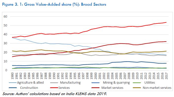 We observe that the value-added share of agriculture & allied activities has declined steadily over the past four decades. It has declined from 36 per cent in 1980 to 18 per cent in 2017. On the contrary, the share of services sector increased from 37 per cent in 1980 to 53 per cent in 2017. The share of non-market services, which consists of public administration, education and health services, remained stagnant around 20 per cent over the entire period whereas the share of market services, which constitute trade, transportation, business and financial services, has increased from 15 per cent to 32 per cent. The increase in share of market services mirrored in an increase in the overall services share. Except for a slight increase during the mid-1990s, the share of manufacturing sector in the total GDP has remained stagnant since 1980. There is an improvement in the share of construction — it increased from 5 per cent in 1980 to 10 per cent in 2008 and then fell to 8 per cent in 2017. The share of utilities sector (electricity, gas & water supply) and mining sector remained stable over the entire period. In terms of the percentage distribution of value-added shares across 27 India KLEMS industries, agriculture and allied activities had the highest share of more than 17 per cent of GDP in 2017, followed by trade (10.8 per cent), other services (9.4 per cent), business services (8.4 per cent), and construction (7.8 per cent). However, the share of agriculture and allied activities has been declining sharply since 1980 — it fell by 19 percentage points in close to 4 decades. Within manufacturing industries, chemicals & chemical products, petroleum & nuclear fuel, non-metallic mineral products, electrical & optical equipment, and transport equipment have shown an increasing share. However, increases in the share of these industries were not sufficient to offset the decline in the share of other sectors, resulting in no improvement in the share of manufacturing in the overall economy. Chemicals & chemical products observed highest increase, from 1.2 per cent in 1980 to 2.5 per cent in 2017, whereas textiles & leather has witnessed the highest decline, from 3.7 per cent in 1980 to 2.1 per cent in 2017. | Table 3.1: Industry share in aggregate nominal gross value added (%) | | KLEMS Industry Description | 1980 | 1994 | 2003 | 2008 | 2017 | | Agriculture & allied | 36.3 | 28.8 | 21.4 | 17.9 | 17.2 | | Industry | 26.9 | 30.4 | 29.9 | 33.1 | 29.3 | | Manufacturing | 17.5 | 18.5 | 16.9 | 18.2 | 16.4 | | Food beverages & tobacco | 1.7 | 2.2 | 2.0 | 2.1 | 1.8 | | Textiles & leather | 3.7 | 3.1 | 2.0 | 1.9 | 2.1 | | Wood & wood pdts. | 1.3 | 0.7 | 0.3 | 0.2 | 0.3 | | Pulp & paper pdts. | 0.6 | 0.6 | 0.4 | 0.5 | 0.4 | | Petroleum & nuclear fuel | 0.5 | 1.0 | 1.6 | 1.9 | 1.2 | | Chemicals & chemical pdts. | 1.2 | 1.8 | 2.1 | 2.2 | 2.5 | | Rubber & plastic pdts. | 0.6 | 0.8 | 0.7 | 0.8 | 0.6 | | Non-metallic mineral pdts. | 0.8 | 1.0 | 1.0 | 1.2 | 1.0 | | Basic metals & metal pdts. | 2.7 | 2.9 | 2.9 | 3.0 | 2.0 | | Machinery, n.e.c. | 1.6 | 1.5 | 1.2 | 1.6 | 1.2 | | Electrical & optical eqpt. | 0.7 | 1.0 | 0.8 | 1.1 | 1.0 | | Transport eqpt. | 1.4 | 1.3 | 1.5 | 1.2 | 1.8 | | Other manufacturing | 0.9 | 0.5 | 0.4 | 0.4 | 0.5 | | Non-manufacturing industries | 9.4 | 11.9 | 13.0 | 15.0 | 12.8 | | Mining & quarrying | 1.9 | 2.7 | 2.8 | 3.2 | 2.3 | | Utilities | 2.1 | 3.5 | 2.9 | 2.1 | 2.7 | | Construction | 5.4 | 5.7 | 7.3 | 9.7 | 7.8 | | Services | 36.8 | 40.8 | 48.8 | 48.9 | 53.5 | | Market services | 15.2 | 20.9 | 28.5 | 29.5 | 32.1 | | Trade | 6.9 | 7.8 | 9.1 | 9.3 | 10.8 | | Hotels & restaurants | 0.6 | 0.7 | 1.0 | 1.1 | 1.0 | | Transport & Storage | 3.3 | 4.7 | 5.5 | 5.0 | 4.8 | | Post & telecom | 0.7 | 1.7 | 2.1 | 2.1 | 1.6 | | Financial services | 2.7 | 4.2 | 5.6 | 6.1 | 5.4 | | Business services | 1.0 | 1.9 | 5.2 | 5.9 | 8.4 | | Non-market services | 21.6 | 19.9 | 20.3 | 19.4 | 21.4 | | Public administration | 5.2 | 5.5 | 6.1 | 5.9 | 6.2 | | Education | 2.0 | 2.3 | 3.0 | 3.0 | 4.1 | | Health | 0.8 | 1.0 | 1.5 | 1.4 | 1.7 | | Other services | 13.6 | 11.1 | 9.6 | 9.2 | 9.4 | | Total economy | 100.0 | 100.0 | 100.0 | 100.0 | 100.0 | | Source: Authors’ calculations based on India KLEMS data 2019. | Clearly, services sector has been the single largest contributor to value added in the post-1980 period. In terms of value-added share in 2017, out of the top 10 industries, 7 industries are from services sector. The steep increase in share of services between 1994 and 2003 is due to expansion of the market services, of which trade, business services, financial services and transport & storage had high value-added shares in all five years. The share of business services had risen sharply from 1 per cent in 1980 to 8.4 per cent in 2017, followed by trade (increased from 6.9 per cent to 10.8 per cent) and financial services (increased from 2.7 per cent to 5.4 per cent). Value added share of non-market services remained constant. Within non-market services, education, health, and public administration observed an increase in value-added shares between 1980 and 2017, while other services recorded a decline. 3.3 Aggregate value-added growth and industry and broad sector contributions to aggregate growth This section presents the growth rate of value added in the aggregate economy, broad sectors of the economy, and detailed 27 KLEMS industries. The first two—the aggregate economy and broad sector growth rates for this chapter—are obtained as Tornqvist aggregates of industry value-added growth rates. In a Tornqvist aggregation approach, the growth rate of each industry value added is weighted by the nominal value-added share of that industry while calculating the aggregate value-added growth rate. Another commonly used approach is to simply sum the real value added across industries to obtain aggregate value added and compute the growth rate—an approach often called the aggregate production function approach (see Jorgenson et al., 2007). The Tornquvist approach, which is consistent with the aggregate production possibility frontier approach described in Jorgenson et al. (2007), relaxes several assumptions in the aggregate production function approach, such as a common production function across all industries. | The aggregate economy and broad sector growth rates have been obtained as Tornqvist aggregates of industry value-added growth rates. |
Figure 3.2 provides the annual growth rate of aggregate value added during 1980-2017, and Table 3.2 provides the average growth rates for the aggregate economy and broad sectors for the four sub-periods and the entire period. On average, the Indian economy grew at 6 per cent per annum during 1981 to 2017. The annual economic growth rate fell sharply in 1991 due to a balance of payment crisis. It subsequently recovered and it grew steadily till 1996 at the time of the East Asian financial crisis—when it slowed until 2002. After that, India witnessed a high growth phase until the global financial crisis in 2007-08. | Table 3.2: Value-added growth rate, Broad Sectors (%) | | Aggregate sectors | 1981-93 | 1994-2002 | 2003-07 | 2008-17 | 1981-2017 | | Agriculture & allied | 3.2 | 2.1 | 4.4 | 3.2 | 3.1 | | Industry | 6.0 | 6.0 | 9.3 | 6.2 | 6.5 | | Manufacturing | 6.1 | 6.1 | 9.2 | 7.2 | 6.8 | | Mining & quarrying | 6.7 | 4.8 | 5.1 | 3.0 | 5.0 | | Utilities | 8.1 | 5.4 | 6.8 | 6.2 | 6.8 | | Construction | 3.9 | 6.1 | 12.0 | 5.2 | 5.9 | | Services | 6.6 | 7.5 | 7.8 | 7.8 | 7.3 | | Market services | 6.7 | 9.8 | 9.8 | 8.2 | 8.2 | | Non-market services | 6.6 | 4.9 | 4.9 | 7.2 | 6.1 | | Total economy | 5.3 | 5.7 | 7.7 | 6.4 | 6.0 | | Source: Authors’ calculations based on India KLEMS data 2019. | The average annual value-added growth rate of the Indian economy was 5.3 per cent during 1981-93. The average annual growth rate in Gross Value Added (GVA) for manufacturing, mining & quarrying, utility, market services and non-market services was between 6.1 and 8.1 per cent, whereas it was 3.2 per cent for agriculture & allied activities and 3.9 per cent for construction. During 1994-2003, GVA growth improved slightly, with construction and market services seeing a rapid rise, even though agriculture & allied activities, mining & quarrying, utilities, and non-market services registered a fall. During the 2003-07 period, when the aggregate economy witnessed a growth acceleration (7.7 per cent per annum), two sectors that registered very impressive growth were manufacturing and construction. The most marked growth acceleration occurred in construction with a trend growth of 12 per cent during 2002-07, while manufacturing observed a jump in growth rate from 6.1 per cent to 9.2 per cent. The growth rate of agriculture & allied activities also accelerated during this period. The overall growth rate declined to 6.4 per cent in the post-financial crisis period and the growth performance of all the broad sectors except non-market services appears similar to the aggregate economy trend. Figure 3.4 shows value added growth rates for 27 industries during 1981-2017. We observe that 19 out of 27 India KLEMS industries grew at a faster rate than the economy (6 per cent per annum). Business services grew the fastest at 11.9 per cent per annum. The other well-performing industries are post & telecommunications, electrical & optical equipment, rubber & plastic, coke & petroleum products, transport equipment, financial services, health & social work, chemicals and chemical products—each growing at more than 8 per cent per annum. At the other end, GVA growth has been quite slow in industries such as, wood & wood products, agriculture & allied activities, mining & quarrying, and other services. The performance of agriculture & allied activities, which is essential for India’s economic growth, was relatively very poor. It is also evident (Annexure Table 3A.1) that there is wide variation in value-added growth rates across the 27 KLEMS industries and across the four sub periods. More industries (10 of 13 that slowed) recorded slower growth in the 1994-2002 sub-period compared to 1981-93, while in the subsequent phase of 2003-07 the slowing was more on account of services—five were services of the seven industries that slowed their pace of growth. | During 1981-2017, 19 out of 27 India KLEMS industries grew in terms of gross value added at a faster rate than the economy (6 per cent per annum). |
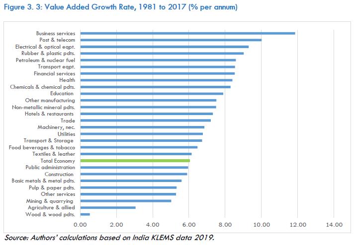 A further comparison between the periods 2003-07 and 2008-16 (Figure 3.5) allows us to identify the industries primarily responsible for the growth slowdown in the 2010s. The industries have been ranked by growth in the 2003-07 period—the highest growth took place in manufacturing industries such as, electrical & optical equipment, pulp & paper products, and machinery n.e.c. Service industries such as, business services, post & telecommunications, hotels & restaurants, health, and construction, witnessed more than 10 per cent per annum growth. At the other end, there are industries such as, wood & wood products, rubber & plastic products, other services, agriculture and allied activities and public administration, which registered less than 5 per cent per annum growth rate during this phase. Value-added growth rates declined over these two sub-periods in most industries. Out of 27 KLEMS industries, only nine recorded increased growth. The decline in growth rate is much more for the industrial sector. So, the improved growth performance of the Indian economy during 2003-07 and economic slowdown after the 2008 financial crisis are largely on account of the manufacturing sector. | The improved growth performance of the Indian economy during 2003-07 and economic slowdown after the 2008 global financial crisis are largely on account of the manufacturing sector. |
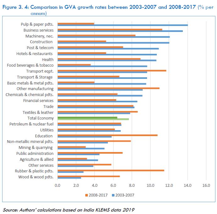 The extent to which an industry can explain differences in aggregate growth does not only depend on its growth rate, but also on its share in value added. Another way to observe this divergence between value-added share and growth in individual industries is to calculate the contribution of each industry to total economic growth. This is done by multiplying individual industry growth with gross value-added share of that industry. In Figures 3.6 and 3.7, we have plotted the contribution of broad sectors and the 27 industries to the aggregate economy GVA growth. As we have seen, services have been the best performing sector in the Indian economy, both in terms of its value-added share and its growth rate. The sector’s contribution to aggregate economic growth more than doubled from 2.1 per cent in 1981 to 4.2 per cent in 2017. The contribution of market services increased significantly from less than 1 per cent in 1981 to 2.4 per cent in 2017. The contribution of manufacturing sector for the entire period has been around 1.2 per cent. Agriculture has contributed less than 0.8 per cent. It is evident from Figure 3.6 that the Indian economy had crossed the barrier of growth of 9.5 per cent in 1988 when agriculture contributed almost 4.4 per cent of the share. Clearly, for the economy to grow at such a rapid pace, such substantive contribution of the agriculture sector was vital. 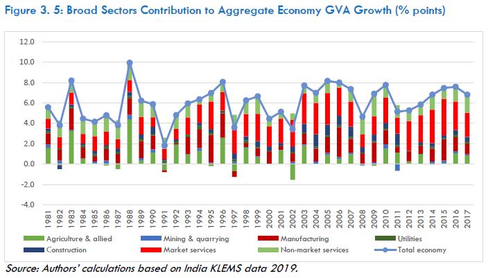 Table 3.3 depicts the sectoral contributions to aggregate value-added growth of the economy. During 1981-93, the service sector contributed about 2.63 percentage points towards the aggregate value-added growth rate of 5.4 per cent. Market and non-market services contributed 1.19 and 1.44 percentage points, respectively and agriculture contributed 1 percentage point. The contribution of industry was 1.72 percentage points, with 1 percentage point coming from the manufacturing sector. The picture changed during the period 1994-2002, when contribution of agriculture and non-market services declined significantly, whereas industry’s contribution remained stagnant. The market services sector did see a significant improvement in its value-added growth contribution—from 1.13 percentage point in the previous period to 2.3 percentage point. Indian economy achieved impressive growth during the 2003-2007 period with improvement from 5.7 per cent to 7.7 per cent. This improvement in GVA growth was reflected in almost all segments of the economy, except in the non-market services. Contribution of manufacturing and construction sector to aggregate value-added growth improved significantly. During 2008-2017, aggregate value-added growth rate declined. In absolute term, the contribution to aggregate GVA growth of all broad sectors except non-market services also declined. | Table 3.3: Contribution to GVA Growth, Broad Sectors (% points) | | Sector | 1981-1993 | 1994-2002 | 2003-2007 | 2008-2017 | 1981-2017 | | Agriculture & allied | 1.00 | 0.57 | 0.87 | 0.57 | 0.76 | | Industry | 1.72 | 1.81 | 2.99 | 1.93 | 1.97 | | Manufacturing | 1.08 | 1.11 | 1.63 | 1.25 | 1.21 | | Mining & quarrying | 0.19 | 0.13 | 0.16 | 0.07 | 0.14 | | Utilities | 0.21 | 0.18 | 0.18 | 0.15 | 0.18 | | Construction | 0.23 | 0.39 | 1.02 | 0.46 | 0.44 | | Services | 2.63 | 3.28 | 3.80 | 3.92 | 3.29 | | Market services | 1.19 | 2.30 | 2.86 | 2.47 | 2.03 | | Non-market services | 1.44 | 0.98 | 0.94 | 1.45 | 1.26 | | Total economy | 5.35 | 5.66 | 7.65 | 6.43 | 6.03 | | Source: Authors’ calculations based on India KLEMS data 2019. | 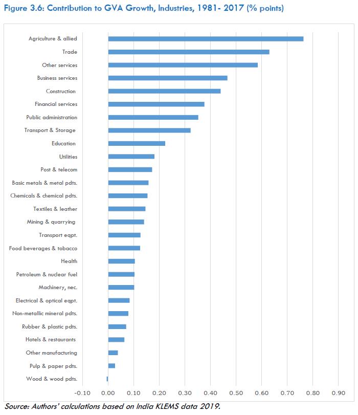 Even though we have observed that Indian agriculture sector grew at 3.1 per cent per annum during the period 1981-2017, in terms of contribution to total value-added growth it has made highest contribution (Figure 3.7), followed by trade. Five important service industries that made substantive contributions are trade, other services, business services, financial intermediation, public administration, and defence—their combined share in value-added was around 40 per cent in 2017. Business services grew at the fastest pace (11.86 per cent per annum) during 1980-2017, while trade and financial services grew at a moderate rate of 7 per cent during the same period. We have seen that service sector contributed around half of the India’s economic growth. But the rise in the overall growth rate during 2003-07 or the fall in the post-financial crisis period stemmed mainly from the industrial sector—specifically from construction and manufacturing. The contribution of agriculture & allied activities and market services to the rise in economic growth rate was much lower. In the post-financial crisis period, all the broad sectors except non-market services observed a decline in the contribution to aggregate economic growth. A further analysis of select industries from the manufacturing and services sectors will help us to identify the industries with substantive potential for growth as well as examine their performance and contribution in terms of economic growth. Veeramani and Dhir (2017) have emphasised that traditional labour-intensive products such as, food products, beverages and tobacco, wood & wood products, pulp & paper products etc., and assembly-related network products such as, electronics and electrical machinery have strong potential for growth. However, we found that the labour-intensive industries such as, wood & wood product and pulp & paper products were the least contributing industries over the last four decades. Based on their shares in value-added, their rates of growth and the potential for growth, we have chosen eight key industries—agriculture; food products, beverages and tobacco; chemicals & chemical products; basic metals & metal products; electrical & optical equipment; business services; financial services and trade. The combined share in value-added of these 8 industries is around 50 per cent. It is to be noted that the decline in value-added share for agriculture & allied activities during the last four decades has been compensated by the other key industries, particularly by the three services industries – trade, financial services & business services. Except for agriculture & allied activities, all other key industries’ growth rate is higher than the aggregate economic growth rate. However, all these industries experienced a slowdown in value-added growth—more so in the manufacturing sector than services in the post-financial crisis period. Electrical & optical equipment recorded the biggest fall in growth rate. Between 1981-93 and 2008-17, the contribution of services increased significantly, albeit not that of manufacturing, even as it decreased for agriculture & allied activities. | Based on their shares in value-added, their rates of growth and the potential for growth, we identified eight key industries—their combined share in value-added is around 50 per cent. |
| Table 3.4: Average Annual GVA Growth, Value Added Share and Industry Contribution to Aggregate GVA growth | | | 1981-1993 | 1994-2002 | 2003-2007 | 2008-2017 | | Average share in value added (percentage) | | Agriculture & allied | 31.5 | 26.0 | 19.7 | 18.1 | | Food beverages & tobacco | 1.9 | 2.0 | 2.1 | 1.9 | | Chemicals & chemical pdts. | 1.4 | 2.0 | 2.1 | 2.3 | | Basic metals & metal pdts. | 2.8 | 2.8 | 3.1 | 2.6 | | Electrical & optical eqpt. | 0.9 | 0.8 | 0.9 | 1.0 | | Trade | 7.4 | 8.3 | 9.4 | 10.0 | | Financial services | 3.2 | 4.8 | 5.5 | 5.8 | | Business services | 1.4 | 3.0 | 5.6 | 6.5 | | Aggregate of above-mentioned industries | 50.4 | 49.7 | 48.4 | 48.2 | | Growth in value added (annual growth) | | Agriculture & allied | 3.2 | 2.1 | 4.4 | 3.2 | | Food beverages & tobacco | 7.7 | 6.2 | 9.7 | 3.6 | | Chemicals & chemical pdts. | 9.7 | 7.8 | 9.1 | 6.5 | | Basic metals & metal pdts. | 4.1 | 7.3 | 9.5 | 4.0 | | Electrical & optical eqpt. | 7.3 | 8.7 | 19.3 | 7.4 | | Trade | 5.4 | 8.1 | 8.3 | 8.2 | | Financial services | 10.1 | 8.6 | 8.6 | 6.3 | | Business services | 8.8 | 16.1 | 13.5 | 11.3 | | Total economy | 5.3 | 5.7 | 7.7 | 6.4 | | Contribution to aggregate value-added growth (per centage points) | | Agriculture & allied | 1.0 | 0.6 | 0.9 | 0.6 | | Food beverages & tobacco | 0.1 | 0.1 | 0.2 | 0.1 | | Chemicals & chemical pdts. | 0.1 | 0.2 | 0.2 | 0.2 | | Basic metals & metal pdts. | 0.1 | 0.2 | 0.3 | 0.1 | | Electrical & optical eqpt. | 0.1 | 0.1 | 0.2 | 0.1 | | Trade | 0.4 | 0.7 | 0.8 | 0.8 | | Financial services | 0.3 | 0.4 | 0.5 | 0.4 | | Business services | 0.1 | 0.5 | 0.7 | 0.8 | | Source: Authors’ calculations based on India KLEMS data 2019. | The above data analysis establishes that while agriculture & allied activities and the industrial sector contributed significantly towards high economic growth during 2003-07, it is the market services sector which grew steadily over the last four decades. Within the market services, business services and trade contributed the most. 3.4 Growth of industry output and intermediate inputs This section presents an analysis of gross output and intermediate input series for the 27 KLEMS industries, in terms of growth of gross output and intermediate input and contribution of intermediate input to gross output growth. Figure 3.7 and Table 3.5 present the average annual growth rates of gross output of the 27 KLEMS industries. For all 27 industries, the average growth rate of output was 7.39 per cent per annum and of these, 12 industries grew faster than the industry average. Output growth is found to be most rapid in business services (12.40 per cent). Of the five fastest growing industries, two are producers of services (business services and post & telecommunication) and three are in manufacturing (electrical & optical equipment, manufacturing n.e.c., rubber and plastic products). All five posted growth rates of over 9.97 per cent during the period 1981-2017. At the other end, output growth has been quite slow for wood & wood products and agriculture and allied activities. | Table 3.5: Average Annual Growth Rates in Gross Output (% per annum) | | KLEMS Industry Description | 1981-1993 | 1994-2002 | 2003-2007 | 2008-2017 | | Agriculture & allied | 2.64 | 2.13 | 3.83 | 3.14 | | Mining & quarrying | 7.31 | 3.97 | 5.63 | 4.46 | | Food beverages & tobacco | 7.35 | 7.89 | 11.66 | 5.60 | | Textiles & leather | 6.36 | 4.89 | 9.78 | 9.55 | | Wood & wood pdts. | -3.14 | -0.15 | 3.01 | 7.01 | | Pulp & paper pdts. | 6.67 | 2.24 | 14.88 | 5.63 | | Petroleum & nuclear fuel | 6.92 | 7.90 | 4.35 | 4.25 | | Chemicals & chemical pdts. | 8.78 | 7.71 | 9.30 | 5.29 | | Rubber & plastic pdts. | 12.04 | 7.63 | 5.60 | 12.67 | | Non-metallic mineral pdts. | 8.80 | 8.10 | 6.18 | 8.56 | | Basic metals & metal pdts. | 6.08 | 6.58 | 13.08 | 6.31 | | Machinery, n.e.c. | 6.11 | 5.46 | 11.75 | 9.78 | | Electrical & optical eqpt. | 9.04 | 8.86 | 20.63 | 10.92 | | Transport eqpt. | 7.81 | 9.33 | 4.99 | 12.25 | | Other manufacturing | 9.04 | 9.15 | 16.85 | 12.47 | | Utilities | 9.79 | 6.59 | 1.98 | 7.47 | | Construction | 3.72 | 7.42 | 12.11 | 4.75 | | Trade | 4.71 | 7.12 | 8.18 | 9.17 | | Hotels & restaurants | 4.57 | 10.36 | 10.99 | 1.73 | | Transport & Storage | 6.53 | 7.59 | 9.20 | 6.27 | | Post & telecom | 7.09 | 18.08 | 11.69 | 5.54 | | Financial services | 9.86 | 9.62 | 7.33 | 7.13 | | Business services | 10.26 | 16.39 | 12.35 | 11.60 | | Public administration | 5.67 | 5.79 | 5.34 | 6.72 | | Education | 5.39 | 8.29 | 5.73 | 11.76 | | Health | 3.95 | 5.39 | 10.80 | 9.11 | | Other services | 7.13 | 3.19 | 3.60 | 6.64 | | Industry Mean | 6.68 | 7.32 | 8.92 | 7.62 | | Source: Authors’ calculations based on India KLEMS data 2019. | Table 3.5 depicts annual average growth rates of output for the four sub periods under consideration. During 1981-93, the best performing industry was rubber and plastic products, growing at the average annual rate of approximately 12 per cent per annum. Five other industries, two of which were from manufacturing—electrical & optical equipment and other manufacturing—grew at the average annual rate of more than 9 per cent per annum. Business services was the only service sector industry which grew at more than 10 per cent per annum, followed by financial services (9.9 per cent per annum). During 1994-2002, all the services except other services and financial services registered higher growth rates compared with the previous sub-period. However, within manufacturing, output growth of six industries improved, while that of seven industries declined. During 2003-07, as many as half the industries achieved their highest output growth, reinforcing the rapid growth achieved by the Indian economy during this period. Among these, electrical & optical equipment, manufacturing n.e.c., pulp, paper & paper products, basic metal & fabricated metal products, construction, machinery, n.e.c., food products, beverages & tobacco, hotels & restaurants, and health & social work registered above 10 per cent growth rates. During 2008-17, growth in gross output accelerated for transport equipment, rubber & plastic product, education, wood & wood products, public administration, and trade. At the other end, the lowest growth rates were observed for hotels & restaurants, coke & petroleum products, chemicals & chemicals products, post & telecommunication, food products, beverages & tobacco, and transport & storage. Table 3.6 shows the annual average growth of gross output, intermediate inputs and three categories of intermediate inputs—material, energy, and service—for all 27 industries. There was wide variation across industries with the growth rate of input ranging from 15.7 per cent in business services to 2.1 per cent in agriculture and allied sector. The growth in intermediate input was relatively faster in business services, manufacturing n.e.c., post & telecommunications, financial services, electrical & optical equipment and relatively very slow in agriculture and allied, wood & wood products, health & social work, coke & petroleum products, and hotels & restaurants. Comparing output growth with input growth, we observe a strong positive correlation between gross output and intermediate input growth (Figure 3.8)—the fastest-growing industries in terms of input growth were also among the fastest in gross output growth. | Table 3.6: Average Annual Growth Rates of Gross Output & Intermediate Inputs, 1981-2017 (% per annum) | | KLEMS Industry Description | Output Growth | Intermediate Input | Material Input | Energy Input | Services Input | | Agriculture & allied | 2.8 | 2.1 | 1.0 | 4.0 | 4.2 | | Mining & quarrying | 5.5 | 8.6 | 10.1 | 4.9 | 8.9 | | Food beverages & tobacco | 7.6 | 7.4 | 7.3 | 5.7 | 8.2 | | Textiles & leather | 7.3 | 7.3 | 8.3 | 5.1 | 5.7 | | Wood & wood pdts. | 1.2 | 2.3 | 2.9 | -0.8 | 1.3 | | Pulp & paper pdts. | 6.4 | 7.1 | 7.6 | 5.9 | 5.9 | | Petroleum & nuclear fuel | 6.1 | 5.8 | 5.9 | 7.9 | 5.3 | | Chemicals & chemical pdts. | 7.7 | 8.2 | 9.8 | 3.4 | 4.8 | | Rubber & plastic pdts. | 10.3 | 9.2 | 10.1 | 7.0 | 7.2 | | Non-metallic mineral pdts. | 8.2 | 8.4 | 10.3 | 7.5 | 6.2 | | Basic metals & metal pdts. | 7.2 | 7.1 | 7.4 | 6.2 | 6.4 | | Machinery, n.e.c. | 7.7 | 6.6 | 7.1 | 4.2 | 5.4 | | Electrical & optical eqpt. | 11.1 | 9.6 | 10.1 | 8.2 | 8.7 | | Transport eqpt. | 9.0 | 8.5 | 8.8 | 9.0 | 7.7 | | Other manufacturing | 11.1 | 10.5 | 11.0 | 8.1 | 9.4 | | Utilities | 7.3 | 6.7 | 4.6 | 7.7 | 8.8 | | Construction | 6.0 | 7.5 | 7.2 | 7.5 | 7.9 | | Trade | 7.0 | 6.6 | 8.7 | 9.7 | 6.0 | | Hotels & restaurants | 6.1 | 5.9 | 5.9 | 3.8 | 6.3 | | Transport & Storage | 7.1 | 8.2 | 7.2 | 8.8 | 8.6 | | Post & telecom | 10.0 | 10.4 | 12.6 | 10.5 | 6.9 | | Financial services | 8.7 | 9.6 | 10.6 | 11.4 | 9.2 | | Business services | 12.4 | 15.7 | 13.6 | 17.3 | 15.8 | | Public administration | 5.9 | 6.1 | 7.1 | 5.0 | 6.0 | | Education | 7.9 | 8.3 | 5.4 | 11.8 | 10.0 | | Health | 6.6 | 5.6 | 6.5 | 4.1 | 2.2 | | Other services | 5.6 | 7.5 | 5.9 | 8.0 | 11.2 | | Industry Mean | 7.4 | 7.7 | 7.9 | 7.1 | 7.2 | | Source: Authors’ calculations based on India KLEMS data 2019. | The growth rates of material, energy and service inputs show considerable variation across industries. The fastest-growing industries in terms of material input were business services, post & telecommunications, manufacturing, n.e.c., financial services, other non-metallic mineral products, mining & quarrying, rubber & plastic products, and electrical & optical equipment. At the other end, material input growth was slow in agriculture and allied, wood and wood products, electricity, gas & water supply, education, and hotels & restaurants. The growth in energy input was highest in business services, education, financial services, post and telecommunications, and trade, was negative in wood & wood products, and almost stagnant in chemicals & chemicals products, hotels & restaurants, and agriculture. The growth rate of services input was high in business services, other services, education, manufacturing n.e.c. and financial services, and very low for wood & wood products, health and social work, agriculture, and chemicals & chemicals products. 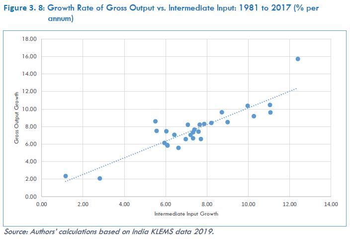 The contribution of an input is measured as the product of an input’s share in value-added and its growth rate. Thus, each input contributes to output in proportion to its value-added share. The estimated factor income shares in gross output for 27 industries are presented in Table 3.7. While estimates have been made for all the years from 1981 to 2017, the table reflects only the period averages. We find that the share of intermediate inputs in gross output is relatively high in all manufacturing industries, electricity, gas & water supply, construction and two services industries viz., hotels & restaurants and post & telecommunication. Among intermediate inputs, material input share is high for all these industries including health & social work, followed by services input share and energy input share. | Table 3.7: Factor Income Shares in Gross Output: 1981 to 2017 | | KLEMS Industry Description | Value Added Share | Material Input | Energy Input | Services Input | | Agriculture & allied | 0.73 | 0.20 | 0.02 | 0.06 | | Mining & quarrying | 0.63 | 0.17 | 0.08 | 0.12 | | Food beverages & tobacco | 0.22 | 0.58 | 0.02 | 0.18 | | Textiles & leather | 0.33 | 0.44 | 0.05 | 0.19 | | Wood & wood pdts. | 0.41 | 0.43 | 0.01 | 0.14 | | Pulp & paper pdts. | 0.34 | 0.43 | 0.07 | 0.16 | | Petroleum & nuclear fuel | 0.12 | 0.83 | 0.02 | 0.03 | | Chemicals & chemical pdts. | 0.30 | 0.49 | 0.07 | 0.15 | | Rubber & plastic pdts. | 0.30 | 0.50 | 0.04 | 0.16 | | Non-metallic mineral pdts. | 0.39 | 0.28 | 0.15 | 0.18 | | Basic metals & metal pdts. | 0.28 | 0.43 | 0.11 | 0.17 | | Machinery, n.e.c. | 0.36 | 0.46 | 0.03 | 0.15 | | Electrical & optical eqpt. | 0.31 | 0.48 | 0.03 | 0.19 | | Transport eqpt. | 0.26 | 0.49 | 0.05 | 0.19 | | Other manufacturing | 0.39 | 0.43 | 0.02 | 0.16 | | Utilities | 0.35 | 0.29 | 0.17 | 0.19 | | Construction | 0.36 | 0.42 | 0.02 | 0.21 | | Trade | 0.76 | 0.04 | 0.02 | 0.18 | | Hotels & restaurants | 0.26 | 0.54 | 0.04 | 0.16 | | Transport & Storage | 0.46 | 0.15 | 0.18 | 0.21 | | Post & telecom | 0.39 | 0.34 | 0.08 | 0.19 | | Financial services | 0.76 | 0.04 | 0.02 | 0.18 | | Business services | 0.66 | 0.10 | 0.02 | 0.22 | | Public administration | 0.73 | 0.04 | 0.00 | 0.22 | | Education | 0.84 | 0.06 | 0.00 | 0.09 | | Health | 0.52 | 0.34 | 0.01 | 0.13 | | Other services | 0.84 | 0.10 | 0.00 | 0.05 | | Source: Authors’ calculations based on India KLEMS data 2019. | Figures 3.9, 3.10 and 3.11 rank the industries in terms of the contributions of material, energy and services input. The mean contributions of these inputs are 2.63, 0.35 and 1.18 percentage points respectively for the period 1981 to 2017. While comparing the contribution of factor inputs—material, energy, services, labour and capital, we found that material input is the dominant source of growth for a majority of the industries. The contribution of energy and services input to output growth has been relatively low as compared to that of material input. Except for agriculture and allied sector and some services (trade, financial services, business services, public administration, education, health, and other services) more than 50 per cent output growth was achieved because of growth in intermediate inputs Material input contributed significantly to gross output growth in certain industries such as, manufacturing n.e.c., coke & petroleum products, rubber & plastic products, electrical & optical products, chemical products. The industries where the contribution of material input to output growth was less than 0.5 percentage points are agriculture, education, trade, public administration, and financial services. The contribution of energy input was the highest in transport & storage, electricity, gas & water supply and other non-metallic mineral products and services input contribution to output growth was the highest in business services, transport & storage, manufacturing n.e.c., electricity, gas & water supply, and financial services.
3.5 Summary and Conclusion The main objective of the India KLEMS project was to construct gross value-added, gross output, labour input, capital service input, intermediate inputs (energy, material, and services) and total factor productivity series of 27 India KLEMS industries from 1980 to 2017. Chapter 2 presented the basic data sources and methodology for building a time series of gross value added, gross output, material, energy, and services input from 1980 to 2017 for 27 industries comprising the Indian economy by using NAS and Input Output Transactions Table (IOTT) data. Based on the constructed time series, this chapter has analysed the trend growth of GVA, GVO and intermediate inputs—materials, energy and services input for 27 industries of the Indian economy for the period 1980-2017. We have done this in two parts—first, we analyse the structure and trends at the level of disaggregated 27 industries as well as at the level of the broad sectors of the economy. In the second part, we have examined the growth rate of gross output and intermediate inputs—materials, energy and services inputs, and analysed the contribution of intermediate inputs in output growth. One of the most interesting features of the Indian economy since 1980s is the emergence of services as the dominant sector and as the main driver of GDP growth. Among fast-growing developing countries, India is distinctive for the role played by the service sector. Whereas earlier developers grew on the basis of exports of labour-intensive manufactures, India has concentrated on services. Although there are other emerging markets where the share of services in GDP exceeds the share of manufacturing, India stands out for the size and dynamism of its service sector. India’s service sector observed an increase in its share in aggregate GVA from nearly 37 percent to more than 53 percent between 1980 and 2017. The share of agriculture in aggregate GVA declined by 19 percentage points and that of manufacturing remained at around 17 per cent during the period. In terms of GVA shares of 27 industries in 2017, although agriculture and allied activities share declined by 19.1 percentage points, it was still the largest sector with 17.2 per cent share in 2017. Further, seven of the top 10 industries in terms of GVA share were from the service sector. We observe that the Indian economy grew at 6.03 per cent per annum during 1981 to 2017 and the growth improved over different sub-periods until the 2008 global financial crisis. While growth in aggregate value-added the Indian economy was between 5 to 6 per cent during 1981-2002, it improved to 7.65 per cent during 2003-07, and then declined slightly to 6.43 per cent in the subsequent sub-period. In terms of broad sectors, services grew at a faster rate (7.31 per cent per annum) than others, while agriculture grew at a much slower rate (3.06 per cent per annum). Market services such as business services, post & telecommunication, and financial services registered much faster growth than non-market services industries such as, health & social work and education & public administration. Within the manufacturing sector, electrical & optical equipment, rubber & plastic products, coke & petroleum products, and transport equipment grew faster than other industries. Of the average growth of 6.03 per cent per annum for the aggregate economy during 1981-2017, 2.03 percentage points came from market services, 1.21 and 1.26 percentage points from manufacturing and non-market services respectively, and less than 0.8 percentage points from agriculture and allied sector. Within the market services, business services and trade contributed most. | Although there are other emerging markets where the share of services in GDP exceeds the share of manufacturing, India stands out for the size and dynamism of its service sector | Our analysis reveals a more prominent effect of the global financial crisis at the disaggregate industry level. For as many as 19 of the 27 KLEMS industries, growth rates declined after 2007-08. The annual growth rate of gross output varied across industries ranging from 1.16 per cent in wood & wood products to 12.4 per cent in business services. Out of 27 industries, 12 observed higher growth rates compared with the industry mean— among them, eight industries are from the manufacturing sector. Agriculture and mining grew at much slower rates than the industry mean of 7.39 per cent per annum, respectively 2.81 and 5.50 per cent. Positive correlation between gross output and intermediate input growth is also observed. In context of the contributions of intermediate inputs to growth in gross output, we observe that, in general, contribution of materials input is higher than the other factors of production. It is as high as 40 to 50 per cent in the case of manufacturing industries. Except for transportation & storage, electricity, gas & water supply, non-metallic mineral and metal products, the contribution of energy input is negligible (less than 3 per cent), while the contribution of service inputs to gross output lies between 10 to 20 per cent. Evidently, the contribution of intermediate input, particularly material input, remained the dominant source of output growth for most industries. Therefore, intermediate inputs play a crucial role in explaining economic growth at the industry level, which is why, we have argued for the use of gross output instead of value-added in productivity analysis. | Intermediate inputs play a crucial role in explaining economic growth at the industry level, which is why, we have argued for the use of gross output instead of value-added in productivity analysis. | Annexure 3A: Additional Table | Table 3A.1: Average Growth Rates of Gross Value Added (% per annum) | | KLEMS Industry Description | 1981-1993 | 1994-2002 | 2003-2007 | 2008-2017 | | Agriculture & allied | 3.2 | 2.1 | 4.4 | 3.2 | | Mining & quarrying | 6.7 | 4.8 | 5.1 | 3.0 | | Food beverages & tobacco | 7.7 | 6.2 | 9.7 | 3.6 | | Textiles & leather | 5.2 | 3.8 | 7.8 | 8.6 | | Wood & wood pdts. | -2.7 | -2.7 | 2.5 | 6.7 | | Pulp & paper pdts. | 6.0 | 1.0 | 14.0 | 3.9 | | Petroleum & nuclear fuel | 12.5 | 5.8 | 6.9 | 6.8 | | Chemicals & chemical pdts. | 9.7 | 7.8 | 9.1 | 6.5 | | Rubber & plastic pdts. | 10.9 | 7.1 | 2.8 | 11.5 | | Non-metallic mineral pdts. | 7.5 | 8.2 | 5.4 | 7.9 | | Basic metals & metal pdts. | 4.1 | 7.3 | 9.5 | 4.0 | | Machinery, n.e.c. | 5.0 | 4.9 | 12.1 | 8.4 | | Electrical & optical eqpt. | 7.3 | 8.7 | 19.3 | 7.4 | | Transport eqpt. | 5.3 | 9.0 | 9.6 | 11.7 | | Other manufacturing | 6.4 | 4.4 | 9.2 | 11.0 | | Utilities | 8.1 | 5.4 | 6.8 | 6.2 | | Construction | 3.9 | 6.1 | 12.0 | 5.2 | | Trade | 5.4 | 8.1 | 8.3 | 8.2 | | Hotels & restaurants | 5.9 | 9.9 | 10.7 | 5.2 | | Transport & Storage | 5.6 | 6.8 | 9.6 | 6.7 | | Post & telecom | 6.8 | 17.4 | 10.9 | 7.1 | | Financial services | 10.1 | 8.6 | 8.6 | 6.3 | | Business services | 8.8 | 16.1 | 13.5 | 11.3 | | Public administration | 5.7 | 6.0 | 4.5 | 7.0 | | Education | 6.1 | 8.4 | 5.8 | 10.8 | | Health | 7.0 | 8.5 | 10.6 | 8.9 | | Other services | 7.1 | 2.8 | 3.9 | 5.8 | | Source: Authors’ calculations based on India KLEMS data 2019. |
Chapter 4: Employment, Labour Quality and Labour Income Share 4.1 Introduction Providing gainful employment to its workforce has always been an integral aspect of economic development in any country, be it a developed or a developing one. However, the problem of job creation has been worsening in several countries owing to multiple factors, including changes in the structure of the labour market. According to ILO (2014), the process of globalisation has also aided the ‘precarisation’ of labour in many countries. India has not remained unaffected by labour market changes and faces similar employment challenges. The Indian economy has experienced some structural transformations in both GDP and employment after the 1990s economic reforms. However, the structural transformation in employment has been slow as compared to that in GDP (Kochhar et al., 2006; Islam, 2008; Papola and Sahu, 2012; Krishna, 2015). The past few years have also created a situation of inadequate job creation despite reasonably strong economic growth. India’s GDP grew at an average rate of 7.3 per cent over the of the period 2014-18, but this growth did not create enough jobs--the increase in employment has not been commensurate with the increase in the workforce. The Indian economy has been slowing since 2016-17 with a continuous fall in its GDP growth rate from 8.26 per cent to 6.8 per cent per annum during 2017-18 and the total unemployment rate by usual status has gone up significantly from 2.2 per cent in 2011-12 to 6.1 per cent in 2017-18. During the same period, the youth unemployment rate (15-29 years) also shot up across all segments--rural and urban, and males and females.55 Some of the reasons pointed out for the recent slowdown in the Indian economy (Nagraj, 2020) are: (i) a decline in the rate of savings and gross capital formation, (ii) unfavourable macro-economic situation with rise in international oil prices, and (iii) a slowdown in GDP of many other countries-post financial crisis of 2008-09, leading to a fall in India’s exports. The challenge then is to bring the Indian economy back to a faster-growth trajectory and accelerate the process of structural transformation. One of the important routes to achieve that objective is through increase in the growth rate of productivity. But an insight into any analysis of productivity requires data on output and inputs--both labour and capital--for the aggregate economy and at the disaggregated industry level. Due to the lack of availability of any such data in a continuous time series, the India KLEMS project, took on the challenge to build a credible time series for the required data, including an employment series.56 Because of the limitations of reliable official data on employment, there are differences of opinion on the actual trend in employment in the recent past. Based on the available data sources, different authors have estimated employment in India for different time periods, but some of these estimates differ from each other (Table 4A.1 in Annexure) mainly due to (i) different estimates of projected population, (ii) use of different employment status and age groups, (iii) different reference periods.57 The sources and problems of employment statistics in India have been widely discussed in the literature (Sivasubramonian; 2004, Himanshu; 2011, Ghose; 2016) and also in chapter 2 of the current report. Based on the employment series constructed for India KLEMS (2019), this chapter discusses trends in employment and the causes underlying slow employment growth in India. Trends in the growth of the labour quality index and labour income share have also been analysed in it. 4.2 Profile of the Workforce since 1980-81 The workforce participation rate (WFPR) of male and female workers employed in Usual Status (usual principal and subsidiary status or UPSS) in rural and urban sectors since 1983 in all major rounds and PLFS (2017-18) are summarised in Table 4.1. It can be observed that the total WFPR was largely stagnant at around 42 per cent between 1983 and 2004-05. There has been a decline since then, and by 2017-18, the figure had declined to as low as 34.7 per cent. On comparing, we observe that the WFPR in urban areas has always been lower than in rural India, but the gap has narrowed down over the period from 10 percentage points in 1983 to just 4 points in 2011-12, and subsequently to only one percentage point in 2017-18. This convergence between the rural and urban sectors has come mainly because of a fall in the rural WFPR by 9 percentage points-from 44.5 per cent to 35 per cent. In general, the WFPR has been much lower among females, both in rural and urban sectors, than among their male counterparts. It was only 16.5 per cent for females against 52 per cent for males in 2017-18. However, while the urban female WFPR has remained stable around 15 per cent, the rural female workforce participation rate has declined by almost half from 34 per cent to 17.5 per cent from 1983 to 2017. | Table 4.1: WPR (per cent) in Usual Status (UPSS) | | | Rural | Urban | All | | Round | Year | Male | Female | Person | Male | Female | Person | Male | Female | Person | | PLFS | (2017-18) | 51.7 | 17.5 | 35.0 | 53.0 | 14.2 | 33.9 | 52.1 | 16.5 | 34.7 | | 68th | (2011-12) | 54.3 | 24.8 | 39.9 | 54.6 | 14.7 | 35.5 | 54.4 | 21.9 | 38.6 | | 61st | (2004-05) | 54.6 | 32.7 | 43.9 | 54.9 | 16.6 | 36.5 | 54.7 | 28.7 | 42.0 | | 55th | (1999-00) | 53.1 | 29.9 | 41.7 | 51.8 | 13.9 | 33.7 | 52.7 | 25.9 | 39.7 | | 50th | (1993-94) | 55.3 | 32.8 | 44.4 | 52.1 | 15.5 | 34.7 | 54.5 | 28.6 | 42.0 | | 43rd | (1987-88) | 53.9 | 32.3 | 43.4 | 50.6 | 15.2 | 33.7 | 53.1 | 28.5 | 41.2 | | 38th | (1983) | 54.7 | 34.0 | 44.5 | 51.2 | 15.1 | 34.0 | 53.8 | 29.6 | 42.0 | | Source: Statement No.10, PLFS report (July 2017-June 2018), p.56 | The figures are to be read along with the explanatory note for comparability (as cautioned by the Government of India in its PLFS Report) A number of explanations have been put forward in the literature for the low WFPR among females. Predominant among them is the ‘distressed employment’ hypothesis, which argues that rural females take up work only during distress and if the economy is doing well, they tend to withdraw from the workforce (Ghose, 2016; Mehrotra and Sinha, 2017). Another plausible explanation is that an increasing number of females are joining and staying in schools and colleges (Mehrotra et al., 2014; Thomas, 2015, Ghose, 2016) or attending to domestic duties (Thomas, 2015). As incomes rise further, a larger proportion of women are seen to work again. Thus, a U-shaped relationship is found between female WFPR and economic development (Tam, 2011). Another explanation focuses on increasing measurement errors in work participation data from the National Sample Surveys (Himanshu 2011; Hirway 2012). Whatever the reasons, the WFPR of females in India is relatively very low-- a mere 27 per cent in 2016, as compared with 80 per cent in Nepal, 67 per cent in Bhutan, 64 per cent in China, 59 per cent in Brazil (Aggarwal and Goldar, 2019). The significant decline in WFPR for females and for all persons in 2017-18 seems to be driven by a significant fall in the rural figures--for both males and females, possibly due to lack of proper employment opportunities, --especially in agriculture and related activities. The reasons for a decline in women participation in the labour market58 also include ‘social restrictions’ on women participation in the labour force, discrimination at workplaces in terms of wages (Srivastava & Srivastava, 2010), getting regular jobs (Goldar & Aggarwal, 2015), and the absence of ample job opportunities for women59 (Thomas, 2015) who are heavily employed in the informal sector without any legal protection. The withdrawal of rural women from the labour force is also prompted by decline in poverty (Ghose, 2016; Mehrotra and Sinha, 2017), and increased migration by men of the households to urban areas in search of jobs that puts family responsibility of childcare and elder care on women. There is thus, a great potential to increase the female WFPR in India by providing employment opportunities in the non-agriculture sectors where, however, the gender disparity is even higher.60 Policy interventions are therefore necessary to bring about the parity. This could happen if improvements are made in women’s access to quality education, suitable training and skill development, improved access to childcare and elder care, improved maternity protection for balancing work-life responsibilities, parental leave, increased job-flexibility, public safety and improved safe and accessible public transport, encouragement to women friendly policies in the private sector, and an awareness about the importance of work by women to their family. These all are to be part of a coordinated policy framework which promotes a pattern of growth that creates job opportunities for women (Aggarwal and Goldar, 2019). The efforts to increase the women WFPR are also imperative so that a sufficient supply of labour is adequately available to meet the growing demand due to a sustained growth in GDP. The WFPR among males is not significantly different between rural and urban sectors and after convergence between the two for the period 1983 to 2005, the urban rate exceeded that in rural sectors. This could be due to faster growth in GDP, especially in the services sector, giving rise to more urban employment opportunities and making urban centres more attractive to migrants. It is not only the level and the structure of employment, which is key to understand the growth process, but its quality as well. Rodgers (2020, p13) points out that the two dimensions of quantity and quality of work need to be considered together as in the ILO’s Decent Work agenda. The concept of quality of employment is multidimensional (Rodgers, 2020) and has been defined on the basis of the nature of employment, the availability of a written job contract, and the social security benefits available in the job (Nayyar, 2012; Papola & Sharma, 2015, Ghose, 2015). Based on these parameters it is perceived that the ‘best’ jobs are regular and salaried ones especially in the formal sector, and the worst ones are the casual jobs in the informal sectors. There are many consequences of increase in ‘informal’61 economy and ‘informal’ employment. Generally, the ‘informal’ activities lack social protection and insurance; have low productivity and low wages; have small-sized enterprises; and are a small contributor to national exchequer because most of these are out of the tax net. With a high share of the employment in the casual and self-employment categories (76.2 percent in 2018), one may infer that the quality of employment in India is still very poor, though there has been a slight improvement in recent years due to an increase in the share of regular employment from 15 percent in 1999 to 23.8 percent in 2018 (Ghose and Kumar, 2021, Table 8). Based on an employment quality index, Ghose and Kumar (2021, p14) also present evidence of a steady improvement in the average quality of employment during 1999-2018, aided by a decline of employment share of the casual labour, and an increase in the employment share of the regular and salary employees. 4.3 Structure and growth in employment 4.3.1 Structure of employment in India during 1980-2017 In this section, we briefly discuss the structural change in employment in India from 1980 to 2017.62 The model for structural change was first developed by Lewis (1954), under which as a country develops, more resources (labour) shift from less productive activities of agriculture sector into activities with higher productivity in the non-agricultural sector in a two-sector economy. Subsequent literature (Kuznets, 1966; Chenery and Syrquin, 1975) extended the structural shift from agriculture to industry and to services and has been discussed by many researchers (Felipe and Estrada, 2008; Felipe et al., 2007; Krishna, et al., 2018; Erumban et.al. 2019). In Table 4.2, we provide the sectoral distribution of employment in India from 1980-81 to 2017-18 to observe how the employment structure has been changing over time. Agriculture now employs just two-fifth of the workforce as compared with 70 per cent in 1980. The size of the agriculture workforce also reduced in absolute numbers for the first time in 2005-06 and has continued to fall since then. However, we find that manufacturing sector experienced a slow growth in employment and while its share increased marginally from 10.4 per cent in 1980 to 11.5 per cent in 2017--the share has remained stagnant since 2003. The combined share of mining and electricity has remained stagnant at around 0.8-0.9 per cent and these two broad sectors do not play any significant role in employment generation in the Indian economy. The maximum growth in employment comes from the construction sector where it increased from just 2 per cent in 1980 to 11.6 per cent in 2017, a sixfold increase with a compound annual growth rate (CAGR) of 6 per cent. Employment in the services sector grew continuously over the period and its share in total employment has doubled from 17 per cent in 1980 to 34 per cent in 2017 with a CAGR of 3.2 per cent (Table 4.3), with the pace of growth being faster in market services (3.7 per cent) than in nonmarket services (2.4 per cent). While the share of employment in market services has increased from 9 per cent to 22 per cent (an increase of 150 per cent), in non-market services it increased from 8 to 12 per cent, i.e., by just 50 per cent. So, the structural change has been such that employment has shifted from agriculture sector to non-agriculture sector, especially to construction and the services sectors. The structural change in employment in India has bypassed the traditional route of agriculture to industry to services and has been a direct shift from agriculture to services. | Table 4.2: Distribution of Employment in broad sectors of the Indian Economy-1980-2017 (%) | | Broad Sectors | 1980-81 | 1994-5 | 2003-04 | 2008-09 | 2017-18 | | Agriculture, Forestry and Fishing | 69.8 | 63.5 | 57.4 | 51.9 | 42.3 | | Mining and Quarrying | 0.5 | 0.7 | 0.6 | 0.6 | 0.4 | | Manufacturing | 10.4 | 10.4 | 11.3 | 11.6 | 11.5 | | Electricity | 0.3 | 0.3 | 0.3 | 0.3 | 0.5 | | Construction | 2.0 | 3.8 | 5.3 | 7.9 | 11.6 | | Services | 16.9 | 21.4 | 25.1 | 27.6 | 33.8 | | Market | 9.1 | 12.6 | 16.0 | 17.8 | 22.2 | | Non-Market | 7.8 | 8.7 | 9.1 | 9.8 | 11.6 | | Total economy | 100.0 | 100.0 | 100.0 | 100.0 | 100.0 | | Source: Authors’ computations from India KLEMS data set (2019) | 4.3.2 Growth in employment In order to have a more detailed understanding of the structural change in employment, we now turn to the analysis of the trend in employment growth in the broad sectors and in 27 India KLEMS industries during the period 1981-2017. The growth in employment for this entire period, along with four sub-periods 1981-93, 1994-2002, 2003-07, and 2008-17 are depicted in Table 4.3 for the seven broad sectors of India’s economy. 4.3.2.1 Growth in Employment in the Broad sectors Table 4.3 shows that over the period 1981-2017, the growth in employment took place at an average rate of just 1.33 per cent per annuum. The share of agriculture sector, which still retains the largest share of employment, has been a laggard with almost zero per cent growth. Among the other broad sectors, growth is driven mainly by the construction sector and the services sector where the average annual growth in employment has been 6 and 3.2 per cent respectively. Within the service sector, it is the market services which have consistently grown faster than the non-market services. Employment growth in construction has been high and it has been able to absorb most of the labour which displaced from agriculture, mainly due to the matching up of the skills in the two sectors. The average annual growth in employment in the manufacturing sector at 1.6 per cent has been quite slow though is still relatively faster than the growth rate in employment in agriculture. It seems manufacturing could not play the role of being the engine of employment growth in the economy. However, the growth in employment has not been uniform across all the sub-periods. Employment growth in agriculture was the highest in the pre-reform period of 1980-93 as the sector was then the major source of employment in the country. However, with the opening up of the economy, opportunities opened up in both manufacturing and in the services sector. This induced labour to move away from agriculture to other greener pastures with higher wages, and perhaps, higher productivity. As a result, job growth in agriculture decelerated after 1993 and in fact, employment declined in absolute numbers leading to a negative employment growth during the sub-periods 2003-07 and 2008-17. We find a similar pattern of employment growth in the mining and quarrying sector. The immediate benefit of economic reforms with removal or relaxation of many licensing rules and lowering of custom duties, was enjoyed by the manufacturing sector and employment during 1994 -2002 grew by 2.4 per cent as compared with 2 per cent during the pre-reform period of 1981-93. Although the growth in employment in manufacturing decelerated a bit during 2003-08, it was still quite impressive at almost 2 per cent. However, the 2008-17 sub-period brought a substantive slowdown to the pace of employment growth in manufacturing, that may be attributed to the impact of the global financial crisis (GFC), increasing international competitiveness and the emergence of strong global value chains (GVC). | Table 4.3: Growth rate of employment in Broad Sectors-1981-1993, 1994-2002, 2003-2007, 2008-2017 and 1981-2017 (per cent per annum) | | Broad Sectors | 1981-93 | 1994-2002 | 2003-07 | 2008-17 | 1981-2017 | | Agriculture, Hunting, Forestry and Fishing | 1.44 | 0.52 | -0.48 | -2.17 | -0.02 | | Mining and Quarrying | 4.27 | 0.15 | -0.12 | -2.83 | 0.76 | | Manufacturing | 2.05 | 2.41 | 1.99 | 0.04 | 1.59 | | Electricity, Gas and Water Supply | 2.58 | 0.99 | 2.98 | 3.93 | 2.61 | | Construction | 6.99 | 4.86 | 8.57 | 4.78 | 6.09 | | Services | 3.73 | 3.52 | 3.00 | 2.34 | 3.20 | | Market Services | 4.39 | 4.35 | 3.38 | 2.50 | 3.74 | | Non-Market Services | 2.88 | 2.20 | 2.33 | 2.02 | 2.41 | | Total economy | 2.11 | 1.60 | 1.27 | 0.12 | 1.33 | | Source: Authors’ computations from India KLEMS data (2019). | The reforms opened the gates for substantive growth in many service sector industries, such as business services, financial services, telecommunication services, other services, etc. but employment generation has not been commensurate. Employment in services grew at a rate of 3.2 per cent during 1981-2017 but the growth has gradually decelerated since 2003. The deceleration is faster for market services (around one percentage point in both the sub-periods of 2003-07 and 2008-17) than non-market services. The construction sector, however, got a boost from expansion of the manufacturing and the services sectors through increasing demand for urban real estate--both housing and commercial, and infrastructure. The construction sector witnessed an expansion of job opportunities and an increase in its share in total employment. Growth in employment in the sector has been very high, especially during the sub-period of 2003-07 due to expansionary fiscal policy of the government, but some slowdown was experienced after the GFC. The overall employment situation has been worsening since 2003, with a deceleration in employment growth. Ghose and Kumar (2021) finds that the deceleration is more for the less-educated (educated only up to primary), indicating a ‘skill-biased’ technological change in the process of production. Post -1999, they find evidence of rapidly declining employment opportunities for less educated workers in both agriculture and non-agriculture sectors. This finding is also supported by what is reflected in Figure 4.3 on the educational distribution of the employed. It highlights that while the share of the ‘less educated’ among total employed persons, has reduced from more than 80 per cent to just around 45 per cent, that of the more educated-- above secondary (or more than 10 years of education) has increased almost four-fold from just 9 per cent to 33 per cent and this process started in the 1990s with the onset of economic reforms. However, Ghose and Kumar (2021) also point out that the increase in employment of more-educated persons was slower than the increase in their working age population. The authors highlight that since 1999, employment elasticity has declined in all the broad sectors, possibly due to increasing mechanisation of agriculture and ‘from any or all of three possible developments: technological advances and associated increases in capital intensity in the constituent (narrowly defined) sub-sectors, changes in the structure of output involving increases in the shares of more technology-and-capital-intensive products, and increase in the share of large enterprises (which generally employ more technology-and-capital-intensive methods of production than small enterprises) in the sector’s output,’63 indicating evidence of rapid technological advances and rising capital intensity in the manufacturing and services sectors. It seems that the 2008 global financial crisis considerably slowed employment growth in the Indian economy because of the domestic and spill over effects of slowdowns observed in many other globally integrated economies. Further discussion on employment growth in India especially in the 2011-2017 period based on an econometric analysis is presented in Annexure 4B. In order to better understand the underlying changes in employment growth within the broad sectors, it will be helpful to next focus on the 27 individual KLEMS industries. 4.3.2.2 Growth in employment in the 27 India KLEMS industries In this section, we discuss the trends in employment growth in the 27 India KLEMS industries during the period 1980-2017. The growth in persons employed for the entire period, 1981-2017, along with four sub-periods 1981-1993, 1994-2002, 2003-2007, and 2008-2017 are depicted in Table 4.4, while Figure 4.1 provides a ranking of the industries according to employment growth for the entire period 1981-2017. From the Table 4.4, we observe that the growth rate of employment varies significantly across industries reflecting a change in the speed at which jobs are created in different sectors during the period. Employment has shifted from farm to the non-farm sector, particularly towards construction and some non-market services such as trade, transport, business and financial services. For the full period of 1980-2017, total employment has increased from 283.6 million to 464.7 million with an average annual growth rate of 1.33 per cent. Meanwhile, agriculture and mining & quarrying, which together employed the largest share of 42.7 per cent of the total employment in 2017, experienced a stagnant growth in employment with almost no annual growth in agriculture and a modest growth of 0.76 per cent in mining. In fact, the agriculture sector employed 1.5 million less persons in 2017 as compared with 1980, and the mining sector provided jobs to only 4.8 lacs extra persons over the 38-year period. Among the 13 KLEMS industries withing manufacturing, very few industries show fast trend growth in employment. As a result, though manufacturing added 24 million jobs between 1980 and 2017, its share in total employment remained relatively stagnant between 10.5-11.5 per cent during the period. Within manufacturing, the industries which have grown at a fast rate, more than 4 per cent per annum, are electrical and optical equipment; machinery, nec; rubber and plastic products; and coke, refined petroleum products (Figure 4.1). At the other extreme, there are industries, mostly the traditional labour-intensive manufacturing industries, where employment growth has been quite slow (at less than 2 per cent) i.e., textiles and leather products; wood and products of wood; food products; other non-metallic mineral products; chemicals; etc. If we wish to increase the share of manufacturing in total employment then some of the slow-growing sectors need policy initiatives and incentives to promote them. Construction is one important sector that has consistently experienced fast employment growth at an average of 6 per cent over the entire period, adding 48 million jobs, which is more than one-fourth of all new jobs added during the period. Though construction has low labour productivity, it has absorbed a major proportion of the displaced labour from agriculture. It now contributes 11.6 per cent to total employment in 2017 as compared with just 2 per cent in 1980. Growth in employment in the construction sector, which has a large share of casual labour, initially accelerated due to expanding government programmes--rural employment guarantee schemes, rural housing schemes and rural roads schemes, but these programmes did not progress much between 2011 and 2018 (Ghose and Kumar, 2021). However, construction still has vast employment potential and can be tapped in the future for more employment opportunities. Most service sub-sectors, except public administration, grew at more than 3 per cent during the 38-year period, resulting in addition of 109 million jobs. Of these, 77 million jobs were added by market services alone. While trade added the maximum number of jobs at 34 million, 17 million jobs were added by transport and storage industry, 14 million by ‘other services’, 13 million by education and 12 million by business services. The service sector thereby contributed 60 per cent to the total additional employment between 1980 and 2017. All activities in the services sector such as trade; hotels; transport; post & telecommunication; financial services; education; and health have registered fast employment growth. Most of this growth can be credited to liberalisation and opening up of the sector after the economic reforms were initiated in 1991.64 However, attention needs to be paid to further tap the employment potential in the services sector, in order to absorb the shift of labour from agriculture. While total employment grew at a substantial rate of 2.1 per cent and 1.6 per cent in the first two sub-periods of 1981-93 and 1994-2002, the rate of growth declined after 2002 -- ending up in an absolute decline in employment of 8 million persons between 2011-12 and 2017-18. In fact, deceleration in the growth in employment could be seen even during the earlier NSS-EUS rounds between 1999-2004 and 2004-11.65 Agriculture and mining also have a negative average employment growth of -1.6 and -1.9 per cent respectively during 2003 to 2017, due to an absolute decline in employment of 57 million in agriculture and 0.6 million in mining. Consequently, their share in total employment has reduced significantly from 58 per cent in 2003 to just 43 per cent in 2017. The deceleration in growth in employment after 2002 is also experienced by many other industries across both, manufacturing and the services sector. Notable among these are: Food products, textiles, wood products, paper products, chemicals, basic metals, trade, hotels, transport, post and telecommunication, public admin., and education. We thus find a widespread phenomenon of falling employment growth. | Table 4.4: Growth rate of employment in 27 industries-1981-1993, 1994-2002, 2003-07, 2008-17 and 1981-2017 (per cent per annum) | | Industry | 1981-93 | 1994-2002 | 2003-07 | 2008-17 | 1981-2017 | | Agriculture, Forestry and Fishing | 1.44 | 0.52 | -0.48 | -2.17 | -0.02 | | Mining and Quarrying | 4.27 | 0.15 | -0.12 | -2.83 | 0.76 | | Food Products, Beverages and Tobacco | 2.79 | 1.39 | 0.77 | -1.24 | 1.09 | | Textiles, Textile Products, Leather and Footwear | 0.52 | 1.98 | 1.76 | -0.92 | 0.65 | | Wood and Products of wood | 1.57 | 4.47 | -1.16 | -4.12 | 0.37 | | Pulp, Paper, Paper products, Printing and Publishing | 2.33 | 4.63 | 1.84 | 0.99 | 2.46 | | Coke, Refined Petroleum Products and Nuclear fuel | 5.70 | 1.89 | 1.69 | 5.19 | 4.09 | | Chemicals and Chemical Products | 3.93 | 1.61 | 0.65 | 0.68 | 2.04 | | Rubber and Plastic Products | 7.39 | 2.33 | 3.85 | 1.93 | 4.20 | | Other Non-Metallic Mineral Products | 1.58 | 2.37 | 3.17 | -1.14 | 1.25 | | Basic Metals and Fabricated Metal Products | 2.24 | 3.16 | 2.15 | 1.88 | 2.36 | | Machinery, nec. | 2.54 | 6.22 | 3.41 | 6.05 | 4.50 | | Electrical and Optical Equipment | 4.96 | 2.30 | 6.83 | 7.38 | 5.22 | | Transport Equipment | 3.74 | 2.54 | 4.03 | 3.28 | 3.36 | | Manufacturing, nec; recycling | 4.04 | 2.36 | 5.44 | -0.29 | 2.65 | | Electricity, Gas and Water Supply | 2.58 | 0.99 | 2.98 | 3.93 | 2.61 | | Construction | 6.99 | 4.86 | 8.57 | 4.78 | 6.09 | | Trade | 4.22 | 3.75 | 2.39 | 1.20 | 3.04 | | Hotels and Restaurants | 2.91 | 5.36 | 4.76 | 2.87 | 3.75 | | Transport and Storage | 4.63 | 4.64 | 3.33 | 2.72 | 3.94 | | Post and Telecommunication | 5.05 | 8.29 | 3.05 | -0.37 | 4.10 | | Financial Services | 6.92 | 2.32 | 5.99 | 3.76 | 4.82 | | Business Service | 7.14 | 10.57 | 9.68 | 8.99 | 8.81 | | Public Administration and Defense; Compulsory Social Security | 1.87 | -0.52 | -1.93 | -0.91 | 0.03 | | Education | 2.84 | 4.75 | 4.59 | 3.34 | 3.68 | | Health and Social Work | 1.81 | 5.10 | 4.33 | 3.83 | 3.50 | | Other services | 3.92 | 2.10 | 2.66 | 1.82 | 2.74 | | Total economy | 2.11 | 1.60 | 1.27 | 0.12 | 1.33 | | Source: Authors’ computations from India KLEMS database (2019). | However, despite low employment growth rate, the unemployment rate has not been high, because of absorption of workers as casual wage labour or as self-employed66, till PLFS (2017-18) when it showed a sharp increase in the open unemployment rate perhaps due to the limit on the absorption capacity of the informal sector (Rodgers, 2020, p.4). Ghose and Kumar (2021), however, argue that the sharp increase in the unemployment rate during 2011-18 was essentially the effect of the sharp decline in the employment rate of the educated, who in the absence of any suitable job opportunities waited for the right employment and joined the ranks of unemployed while the less-educated just opted out of the labour force after losing all hopes of getting work. 4.3.2.3 Some plausible explanations for the slowdown in employment growth India experienced a severe slowing of growth in employment after the global financial crisis (GFC) of 2008, with the average annual growth rate for employment falling from 1.3 per cent for the period 2003-07, to just 0.6 per cent for 2008-17. However, an international comparison shows that India was not alone in experiencing such deceleration (Figure 4.2), with many other countries also facing significant adverse impacts. It is evident that all BRICS countries, and most of the other selected countries of Philippines, Thailand, Vietnam, US and Japan observed a significantly lower growth in employment during 2008-17 as compared with the pre-GFC period of 2003-07. Only few countries, e.g., Bangladesh, Indonesia and Malaysia were able to face the GFC and sustain the pace of growth in employment. 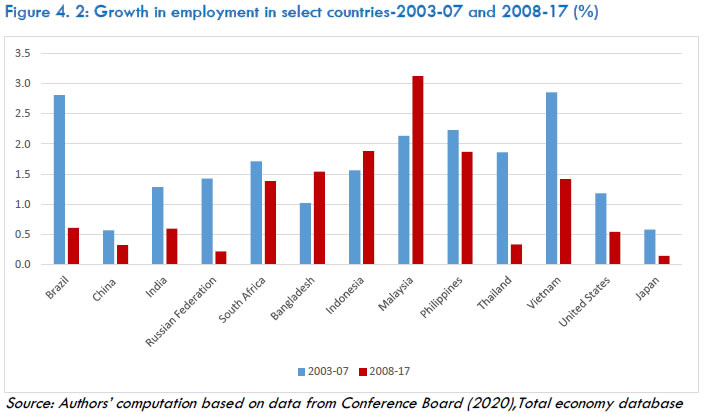 Several explanations have been provided for the low employment growth in India, which include low work-force participation rates (WFPR), low labour intensity in several sectors (Panagariya, 2008), rigid labour laws (Fallon & Lucas, 1991; Besley & Burgess, 2004), increased use of capital- intensive technology (Das et al., 2015; Jha, 2015), rapid advancements in technology, low employment elasticity67, decline in poverty of the households that induces women not to work in low-productive jobs (MGI, 2017) and non-availability of suitable jobs. India is now facing a serious problem with its relatively slow employment growth since 2008. Most sectors have registered a decline in the rate of employment growth since the global financial crisis of 2008.68 The industries of coke, refined petroleum products and nuclear fuel, machinery, nec., electrical and optical equipment, are the few exceptions that have experienced a real surge in employment growth. Dhawan and Sengupta (2020) have identified 11 manufacturing industries, where integration with the global value chains69 could accelerate the growth of output and employment in India. These include auto-vehicles and vehicle components, capital goods, pharma, chemicals, agriculture and food, metals, textiles and apparel, leather and rubber, renewable energy, etc. A meaningful employment policy thus has to be designed which can understand the dynamics of the employment potential of each industry and take necessary sector specific measures to tap their potential. India has to identify the strongest growing industries of the economy, both in manufacturing and modern services and also the skills that are in demand. Skill enhancement and required training for the acquisition of these skills should be the focus of the educational and employment progammes. Since India has not invested enough in the human infrastructure to reap the benefit of its demographic transition, so investment in human and physical infrastructure will need to be scaled up to promote entrepreneurship and create jobs. The next generation of economic reforms necessary to promote and maintain international competitiveness must also be undertaken at the earliest so as to reap the benefits of GVC and the integration of the different economies. 4.4 Growth in Labour Quality Index The discussion about labour quality emanates from the importance of human capital which helps improve the quality of labour input and thus the growth of output through increase in labour productivity. According to the Human Capital Index (World Bank, 2020, pp. ix), ‘human capital consists of the knowledge, skills, and health that people accumulate over their lives. People’s health and education have undeniable intrinsic value, and human capital also enables people to realise their potential as productive members of society. More human capital is associated with higher earnings for people, and higher income for countries.’70 However, growth in labour quality index is mainly a measure of change in the skill composition of the total workforce and total compensation over a period of time. Labour quality though is intertwined with human capital, but it does not directly embody health of the people and is a narrower construct than human capital. The labour quality index is sensitive to the measurement of earnings and the distribution of labour across different categories. Any change in labour quality in India can be partially explained by inter-industry shifts of labour and partially by a change in the composition of labour. The changes in the composition of labour in India are summarised in Figure 4.3, which indicates that there has been an increase in the share of high skilled71 labour (with education above Hr. Sec.) from mere 2.4 per cent to almost 13 per cent between 1983 and 2017-18. It is also evident that the proportion of employed persons with low level of education, i.e., either with below primary level of education or with primary level of education, has consistently decreased over the period along with the increase in high skilled labour. 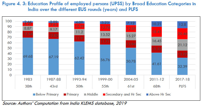 4.4.1 Growth in Labour Quality index in Broad sectors Generally, the index of labour quality improves over time with improvements in the skill level (i.e., with education and experience) of labour. While measuring labour quality is a data-intensive and data accuracy-sensitive exercise, it is also an important exercise given that the quality of labour significantly affects availability of labour input for growth. From Table 4.5, it is evident that during 1981 to 2017, the index of labour quality in India increased at an annual growth rate of 1.2 per cent, which is marginally slower than the growth in employment at 1.3 per cent (Table 4.3). It thus indicates that the growth in labour quality index is almost as important as the growth in employment for growth in labour input. The growth in labour quality index has been relatively fast in mining and manufacturing sectors and has been slow in agriculture and construction sectors. Growth in the index has been moderate for the services sector at an average of 0.9 per cent per year, but the growth rate, as expected, is slightly higher in market services as compared with non-market services. It reflects the skill requirements and the nature of activity of the sectors. Since the growth in labour quality is affected by both the changes in the skill composition (education) and the growth in labour compensation (wages paid to labour), we hardly notice any significant changes in the skill composition of the labour who works in agriculture and construction. It is also clear that growth in labour quality index in most of the broad sectors has been faster in the sub-period 2003-07 as compared with the period 2008-17, possibly due to faster growth in wages during this sub-period. | Table 4.5: Growth in labour quality index in Broad Sectors-1981-1993, 1994-2002, 2003-2007, 2008-2017 and 1981-2017 (per cent per annum) | | KLEMS Industry/Period | 1981-93 | 1994-2002 | 2003-07 | 2008-2017 | 1981-2017 | | Agriculture, Forestry and Fishing | 0.30 | 0.26 | 0.33 | 0.35 | 0.31 | | Mining and Quarrying | 1.18 | 0.48 | 2.67 | 1.59 | 1.32 | | Manufacturing | 1.26 | 0.98 | 1.05 | 1.03 | 1.10 | | Electricity | 0.57 | 1.19 | 0.72 | 0.44 | 0.71 | | Construction | 0.54 | 0.29 | 0.24 | 0.39 | 0.39 | | Services | 1.03 | 0.90 | 1.07 | 0.81 | 0.94 | | Market services | 1.03 | 0.93 | 1.14 | 0.84 | 0.97 | | Non-Market services | 0.89 | 0.95 | 0.84 | 0.74 | 0.86 | | Total economy | 1.24 | 1.11 | 1.29 | 1.11 | 1.18 | | Source: Authors’ computations from India KLEMS database (2019). | 4.4.2 Growth in labour quality index for the 27 India KLEMS industries The growth in labour quality index for the 27 KLEMS industries is presented in Table 4.6 for all the four sub-periods as well as for the entire period of 1981-2017. It shows that the growth in labour quality index over 1981-2017 has wide variations both between industries and also over time within the same industry. While the agriculture sector observed an annual growth of only 0.3 per cent, mining experienced among the highest annual rates of growth of 1.32 per cent across all 27 industries. Within the manufacturing sector, we find that eight out of 13 industries have grown at a rate of 0.7 per cent or higher, e.g., food products, paper products, chemicals, rubber, machinery, transport, while the remaining five have shown a lower growth rate. While the labour quality index in the utility industry grew at an average rate of 0.7 per cent per annum, the growth has been much slower in the construction industry mainly due to the predominance of the low-skilled labour in the construction industry—that is mostly casual labour without any job security, earning very low wages, often even below the statutory minimum wage rates. The industries within the services sector did not experience the similar wide variation in the growth of index of labour quality, mainly because of the similar nature of the skills- mainly medium to high-skill, of the person employed in these industries. On one extreme of the variation, we have ‘other’ services and health with more than or equal to 0.7 per cent annual growth, and on the other extreme the industries of ‘business’ services and financial services observed an annual growth of around 0.4 per cent in labour quality index. On the whole, we find that not only skill quality of each industry is different, but it has changed differently over the whole period and during the sub-periods (Table 4.6) and there is no discernible common pattern during the four sub-periods. | Table 4.6: Growth in labour quality index for 27 industries-1981-1993, 1994-2002, 2003-2007, 2008-2017 and 1981-2017 (percent per annum) | | KLEMS Industry/Period | 1981-93 | 1994-2002 | 2003-07 | 2008-2017 | 1981-2017 | | Agriculture, Forestry and Fishing | 0.30 | 0.26 | 0.33 | 0.35 | 0.31 | | Mining and Quarrying | 1.18 | 0.48 | 2.67 | 1.59 | 1.32 | | Food Products, Beverages and Tobacco | 0.66 | 0.82 | 0.74 | 0.78 | 0.74 | | Textiles, Textile Products, Leather and Footwear | 0.66 | 0.82 | 0.59 | 0.42 | 0.63 | | Wood and Products of wood | -0.57 | 0.72 | 0.54 | 0.45 | 0.17 | | Pulp, Paper, Paper products, Printing and Publishing | 1.01 | 0.87 | 1.20 | 0.22 | 0.79 | | Coke, Refined Petroleum Products and Nuclear fuel | 0.50 | 2.05 | 1.30 | -1.06 | 0.57 | | Chemicals and Chemical Products | 1.26 | 0.81 | 1.21 | 2.02 | 1.35 | | Rubber and Plastic Products | 1.31 | 0.70 | -0.13 | 0.76 | 0.82 | | Other Non-Metallic Mineral Products | 1.22 | 0.14 | 0.36 | 1.02 | 0.79 | | Basic Metals and Fabricated Metal Products | 1.23 | 0.52 | 0.33 | 0.76 | 0.81 | | Machinery, nec. | 2.12 | 1.51 | 0.61 | -0.44 | 1.08 | | Electrical and Optical Equipment | 0.77 | -0.20 | 1.47 | 0.21 | 0.48 | | Transport Equipment | 1.44 | 0.28 | 1.91 | 0.09 | 0.86 | | Manufacturing, nec; recycling | 0.69 | 0.78 | 0.22 | 0.26 | 0.53 | | Electricity, Gas and Water Supply | 0.57 | 1.19 | 0.72 | 0.44 | 0.71 | | Construction | 0.54 | 0.29 | 0.24 | 0.39 | 0.39 | | Trade | 0.71 | 0.72 | 0.57 | 0.41 | 0.61 | | Hotels and Restaurants | 0.29 | 0.73 | 0.80 | 0.51 | 0.53 | | Transport and Storage | 0.63 | 0.69 | 0.67 | 0.42 | 0.59 | | Post and Telecommunication | 0.48 | 0.69 | 1.08 | 0.51 | 0.62 | | Financial Services | 0.77 | -0.06 | 0.51 | 0.35 | 0.42 | | Business Services | 0.21 | 0.57 | 0.86 | 0.16 | 0.37 | | Public Administration and Defense; Compulsory Social Security | 0.81 | 0.31 | 0.80 | 0.48 | 0.60 | | Education | 0.56 | 0.46 | 0.49 | 0.22 | 0.43 | | Health and Social Work | 1.00 | 0.59 | 0.73 | 0.39 | 0.70 | | Other Services | 1.17 | 0.31 | 1.07 | 0.63 | 0.80 | | Total economy | 1.24 | 1.11 | 1.29 | 1.11 | 1.18 | | Source: Authors’ computations from India KLEMS database (2019). | 4.5 Growth in Labour Input The growth rate of labour input, measured as the growth rate in number of persons employed plus growth rate of labour quality index is briefly analysed in this section. 4.5.1 Growth in Labour Input in Broad sectors It is observed that the growth rates of labour input are higher than those of persons employed because of contribution of labour quality index, but the trend in growth in labour input is similar to that of the growth in employment. Like growth in employment, the fastest growth in labour input has been observed by the construction sector, followed by the services sector- induced by acceleration in the market services, and the electricity sector (Table 4.7). | Table 4.7: Growth in labour input in Broad Sectors-1981-1993, 1994-2002, 2003-2007, 2008-2017 and 1981-2017 (percent per annum) | | Broad sectors | 1981-93 | 1994-2002 | 2003-07 | 2008-17 | 1981-2017 | | Agriculture, Hunting, Forestry and Fishing | 1.74 | 0.77 | -0.14 | -1.82 | 0.29 | | Mining and Quarrying | 5.45 | 0.64 | 2.55 | -1.24 | 2.08 | | Manufacturing | 3.31 | 3.39 | 3.04 | 1.07 | 2.69 | | Electricity, Gas and Water Supply | 3.15 | 2.19 | 3.70 | 4.37 | 3.32 | | Construction | 7.53 | 5.14 | 8.80 | 5.16 | 6.48 | | Services | 4.76 | 4.41 | 4.07 | 3.15 | 4.14 | | Market services | 5.42 | 5.28 | 4.52 | 3.34 | 4.71 | | Non-Market services | 3.77 | 3.15 | 3.17 | 2.76 | 3.27 | | Total economy | 3.35 | 2.71 | 2.56 | 1.23 | 2.51 | | Source: Authors’ computations from India KLEMS database (2019). | 4.5.2 Growth in Labour Input for the 27 KLEMS industries The average annual growth rate of labour input for the period 1980-2017 in Figure 4.4 shows that the combined push of the two growth rates led the growth in labour input to be the fastest in business services; construction; electrical and optical equipment; machinery, nec; financial services; rubber and plastic products; and post & telecommunication. On the other hand, there are industries where growth in labour input has been quite slow i.e., agriculture; wood and products of wood; public administration and defence; textiles and leather products; and food products, beverages and tobacco. The growth in labour input is an important indicator for policy makers to pay special attention. to those industries which contribute significantly to labour input growth. 4.6 Labour Income Share The distribution of income between capital, labour and intermediate inputs, is an important element in growth accounting because income shares, under conditions of competitive markets, can be used to measure the contributions that each factor makes towards output growth. So, measurement of labour income share plays an important role in the growth accounting framework to compute total factor productivity (TFP).72 In production analysis, with only two factors of production -- labour and capital, the labour income share is defined as the ratio of labour income to gross value added (GVA). Then, under the assumption of constant returns to scale, the sum of the labour income share and the capital income share is equal to one and the capital income share can be obtained as the residual of one minus the labour income share. The importance of labour income share also lies in understanding the changes in the distribution of national income. A downward trend in the labour income share is an indication that a higher share of national income is going to the capital, thus implying an unequal distribution of national income. However, it is to be noted that since labour income share (SL) is inversely related to labour productivity (LP) (equation 4.3); therefore, its distribution would also help in explaining the pattern of labour productivity.73 So, if product wage rises faster than labour productivity, the labour income share increases. If they move in tandem, the labour income share remains unchanged. Thus, unless the growth in product wages (nominal wages deflated by price index of output) is faster than the growth in labour productivity, the growth in labour income share is bound to be negative. 4.6.1 Trends in labour income share in India For an understanding of the trend in labour income share for the broad sectors of the Indian economy, the results for selected years are presented74 in Table 4.8. While labour income share for each industry is obtained directly from equation 4.1; that for each sector can be defined as the weighted average of each industry’s labour income share (equation 4.4). The weight for each industry is the share of the industry’s value added in the total value added of the sector. Therefore, the trend of total labour income share in a sector (or in the economy) can be decomposed by the change in the labour income share within each industry over the period and the change in value added share of each industry within the sector (or economy). Thus, where Sst and Sit are the labour income share in sector ‘s’ and industry ‘i’ at period t and vit is the share of value added in the ith industry at period t. From Table 4.8 it is clear that the total economy and all the broad sectors have a long-term tendency of a declining trend in labour income share. A closer analysis reveals that in 1980, the labour income share varied from a maximum of 79 per cent in construction to the minimum of 35 per cent in electricity, followed by manufacturing, at 39 per cent and services and agriculture at around 57 per cent each. The non-market services had a higher labour income share, at 61 per cent as compared to 52 per cent for the market services sector. However, by 2017, labour income shares of the total economy and of the services sector had each declined by around four percentage points because of a change in the structure of the economy, by more than half in mining and by eight percentage points in manufacturing. The decline in the labour income share has been sharper for market services, by more than 11 percentage points, as compared to non-market services, which witnessed a decline of just one percentage point. An inter-temporal comparison shows that between 1980 and 2003, the labour income share has declined in the intermediate years for the all the broad sectors and the total economy except the construction sector where it is almost stagnant at around 79 per cent. After 2003, while there is a continuous decline in the share for mining and construction, there was a marginal increase in labour income share for manufacturing and services--both market and non-market. But the share has remained stagnant for agriculture. Though an increase in labour income share of 2.6 percentage points is observed in the total economy between 2008 and 2017, the figure for 2017-18 is still lower than that what it was in 1980-81. The increase between 2008 and 2017 seems to have been induced by an increase in the share for the manufacturing and services sectors. One of the likely reasons for this is the fast increase in real product wages in manufacturing and market services during this period (Table 4.12). Much attention has been paid lately to the falling labour income share in many countries across the world. Dao et al. (2017), point out that there has been a downward trend in labour share in global income since the early 1990s and this downward trend is observed for advanced economies as well as emerging market and developing economies (EMDEs). For India, a decline in the labour income share in manufacturing has been found by a few scholars (Goldar and Aggarwal, 2005; Goldar, 2013; Abraham and Sasikumar, 2017; Goldar, 2022). | Table 4.8: Labour Income Share in Broad Sectors | | Broad Sectors | 1980-81 | 1993-94 | 2002-03 | 2007-08 | 2017-18 | | Agriculture, Forestry and Fishing | 57.6 | 56.1 | 54.8 | 55.1 | 55.9 | | Mining and Quarrying | 58.4 | 30.9 | 29.0 | 27.9 | 29.0 | | Manufacturing | 38.9 | 30.7 | 30.0 | 25.7 | 30.5 | | Electricity | 35.5 | 23.4 | 26.8 | 31.0 | 33.6 | | Construction | 79.1 | 79.9 | 78.4 | 71.3 | 77.5 | | Services | 57.8 | 54.8 | 52.5 | 45.6 | 53.3 | | Market Services | 51.9 | 44.8 | 42.7 | 38.4 | 44.9 | | Non-Market Services | 61.9 | 64.4 | 65.2 | 57.3 | 65.8 | | Total economy | 55.1 | 50.7 | 49.5 | 45.2 | 50.8 | | Source: Authors’ computations from KLEMS data (2019). | 4.6.2 The volatility of the labour income share Based on the notion of constant labour income share advanced by Kaldor (1956, 1961), Solow (1958) proposed two ways to evaluate the stability of the labour income share. The first one is absolute stability, which means to examine the changing extent of total labour income share (expressed by serial variance) in a certain time span. The other one is relative stability, which requires that the variance of total labour income share should be less than the variance in each sector or industry (Zhou, 2016, p.68). We have used the same methodology to explain the volatility in the labour income share through absolute and relative stability. While Table 4.9 shows the results of absolute stability in labour income share for the economy during 1980 to 2017, the results for relative stability are presented in Table 4.10. The results in Table 4.9 do not satisfy the condition of absolute stability and show that the volatility value for the combined period lies, contrary to the theory, outside the volatility values for the sub-periods. | Table 4.9: Comparison of absolute stability of labour income share -1980 to 2017 | | Period→ | Standard deviation
(1980-93) | Standard deviation
(1994-2002) | Standard deviation
(2003-2017) | Standard deviation
(1980-2017) | | Standard Deviation | 0.010 | 0.007 | 0.017 | 0.024 | | Source: Authors’ computations from KLEMS data (2019). | Table 4.10 shows the standard deviations of labour income shares in the total economy and the broad sectors. It is evident that the condition of relative stability is satisfied as it is found that the volatility of the labour income share for the total economy is generally lower than ‘within’ sector volatility, except agriculture.75 The two results together show that although the labour income share in each sector has a relatively larger change, the change of total labour income share can be relatively stable due to the sectoral structure change, but the stability is missing over time. | Table 4.10: Comparison of relative stability of labour income share -1980 to 2017 | | Broad Sectors | Standard Deviation (1980-2017) | | Agriculture, Forestry and Fishing | 0.010 | | Mining and Quarrying | 0.060 | | Manufacturing | 0.037 | | Electricity | 0.060 | | Construction | 0.025 | | Services | 0.036 | | Market Services | 0.035 | | Non-Market Services | 0.027 | | Total economy | 0.025 | | Source: Authors’ computations from KLEMS data (2019). | 4.6.3 Reallocation of change in the labour income share Since the labour income share for the economy is computed by the weighted labour income share of its constituent industries (equation 4.4), the change in the labour income share could be explained either by change in the labour income share of each industry or by the change in the value-added share; i.e., a structural change or by change in both the components.76 Zhou (2016) has used the methodology proposed earlier by Ruiz (2005) and Young (2006) in which the total change is decomposed into three effects--the ‘within’ industry effect; the ‘structural change’ effect (‘between’ effect) and the ‘covariance’ effect. The present chapter has used the equation proposed by Zhou (2016, p.70) for the KLEMS 27 industries and is as follows: 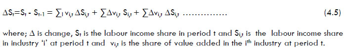 The three effects obtained by using equation 4.5 for the 27 KLEMS industries are depicted in Table 4.11. It shows that the changes in labour income share over the period 1981-2017 have not been uniform. While there has been a general decline of 0.12 percentage points per year over the entire period (Table 4.11), it varies between the different sub-periods of the study. The decline in wage share is observed for the first three sub-periods and is relatively large in sub-period of 2003 to 2007, but the share increased in the fourth sub-period, 2008-2017. For the entire period of 1981-2017 and the first three sub-periods, both within and between industry effects are responsible for the decline in the wage share but within industry effect is greater than the structural effect. In the period of post-GFC, 2008-17, both the effects have actually contributed to the increase in wage share. The result of a stronger within-industry effect than the between-industry effect to explain the change in aggregate labour income share is also supported by Abraham and Sasikumar (2017)77 for Indian organized manufacturing sector, and OECD (2012) for 26 OECD countries and 20 industries in the private sector since 1990. | Table 4.11: Average Change in Labour income share in India (percentage points per year) | | Industry Effect/Period | 1981-1993 | 1994-2002 | 2003-2007 | 2008-2017 | 1981-2017 | | Change in labour income share | -0.34% | -0.13% | -0.85% | 0.55% | -0.12% | | Within Industry Effect | -0.25% | -0.04% | -0.73% | 0.52% | -0.06% | | Structural Effect | -0.01% | -0.03% | -0.08% | 0.10% | 0.00% | | Covariance effect | -0.08% | -0.07% | -0.04% | -0.06% | -0.07% | | Source: Authors’ computations from KLEMS database (2019). | Since it has been noticed from equation 4.3 and the discussion on labour income share that the behaviour of labour income share is induced by the behaviour of real product wages, we present a brief overview of the average growth rates of real product wages for the broad sectors for 1981-2017 and the sub-periods in Table 4.12 and the trends for broad sectors in Figure 4.5, in order to complete the discussion on labour income share. | Table 4.12 : Growth rate in Real Product wages in Broad Sectors-1981-93, 1994-2002, 2003-07, 2008-17 and 1981-2017 (per cent per annum) | | Broad Sectors | Average growth rate
(1981-93) | Average growth rate
(1994-2002) | Average growth rate
(2003-2007) | Average growth rate
(2008-2017) | Average growth rate
(1981-2017) | | Agriculture, Forestry and Fishing | 1.5 | 1.3 | 4.9 | 5.5 | 3.0 | | Mining and Quarrying | -2.5 | 4.0 | 4.5 | 6.2 | 2.4 | | Manufacturing | 2.2 | 3.5 | 4.0 | 8.6 | 4.5 | | Electricity | 2.3 | 6.0 | 6.7 | 3.0 | 4.0 | | Construction | -3.0 | 1.0 | 1.6 | 1.3 | -0.2 | | Services | 2.5 | 2.9 | 1.8 | 7.0 | 3.7 | | Market Services | 1.1 | 4.4 | 4.2 | 7.2 | 4.0 | | Non-Market Services | 4.1 | 2.5 | -0.2 | 6.5 | 3.8 | | Total economy | 2.3 | 3.2 | 4.4 | 7.2 | 4.1 | | Source: Authors’ computations from KLEMS database (2019). | It is evident from Table 4.12 that the total economy has experienced a consistent acceleration in average growth rate of real product wages in all the sub-periods. The same trend is visible in all the broad sectors except electricity and construction where a deceleration in growth in real product wages is observed in the sub-period of 2008-17. The growth in real product wages is almost same for both market and non-market services at four per cent per annum. Another feature is the decline in the level of real product wages in the sub-period 1980-93 in both mining and construction, resulting in a negative average growth rate during 1981-93 and also an overall negative average growth rate for the entire period 1981-2017 for the construction sector, and only a small positive increase in the mining sector. A similar narrative is visible from Figure 4.5 showing a trend in the index of real product wages (the level of real product wages in 1980-81 is taken to be 100) for all the broad sectors. 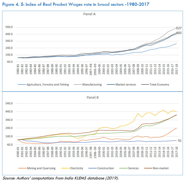 The total economy has observed an increase of 360 per cent in level of real product wages induced by more than 425 per cent increase in the level of wages in the manufacturing sector (Panel A). The slowest increase is evident in the mining sector, and the construction sector- which has actually witnessed a decline in the index of real product wages (panel B). 4.7 Summary and Conclusion The chapter presents an analysis of the trend in time series of persons employed, labour quality index and labour input from 1980 to 2017 for the broad sector of the economy and the 27 KLEMS industries comprising the Indian economy. The main findings of the chapter can be summarised as: (a) The overall WFPR in India has been falling, especially for rural females; (b) There has been a significant change in the structure of employment in the Indian economy between 1980 and 2017-- while the share of agriculture has reduced in total employment from 70 per cent to 42 per cent, the share of the services sector has doubled from 17 per cent to 34 per cent, pushed by a two and a half times increase in the share of market services from 9 per cent to 22 per cent during the same period-- thus establishing that growth has been mainly service-led; (c) The growth in employment has slowed down considerably in the recent period--there has been an absolute decline of 8 million employed persons between 2011-12 and 2017-18--and the unemployment rate has increased significantly during the same period. The employment level declined between 2011 and 2017 in agriculture, mining, as well as in manufacturing and while employment growth has been driven mainly by construction (a sector that had substantially helped absorb labour from agriculture till 2011) and the services sectors, especially market services, this growth has also slowed; (d) A change is noticed in the education profile of the work force as the proportion of more-educated workers has significantly increased; (e) Along with overall growth in employment, there has been a significant growth, at 1.2 per cent per annum, in the labour quality index leading to a faster growth in labour input during 1981-2017. Growth in employment and growth in labour quality index have not been uniform, with considerable variations being observed across industries and across sub-periods in both; (f) Though there is a long-term trend of a fall in labour income share for the economy, no unique trend could be discerned at the broad sector level. The change in labour income share seems to have occurred mainly due to ‘within industry’ effect in the sectors and ‘within industry’ effect is larger as compared with the structural change effect. Real product wages have experienced a consistent increase, with an annual average growth rate of four per cent for the period of 1981-2017. We thus find that India’s employment situation has been quite precarious with an absolute decline in total employment and shooting unemployment rates between 2011-17. However, with a fall in employment elasticity from 0.3-0.4 in 1999 to 0.1 - 0.2 in 2017, unless India achieves a growth rate 8-9 per cent in real GDP that is job-rich, it will not be able to meet the challenge of providing employment to the backlog and the additions to labour force.78 Rather than a macro approach, the key to policymaking appears to lie in a focus on sectoral understanding and microeconomics. Annexure 4A: Additional Tables | Table 4A.1: Summary of Employment estimates by different authors | | S. No. | Author | Year of Publication | Employment Status applied | Age group | 1983 | 1987-88 | 1993-94 | 1999-00 | 2004-05 | 2011-12 | 2017-18 | | 1 | Vasaria, Pravin | 1996 | UPSS | All | 302.3 | 324.6 | 374.4 | NA | NA | NA | NA | | 2 | Sundaram, k | 2007 | UPSS | All | 307.8 | NA | 367.7 | 400.8 | 457.9 | NA | NA | | 3 | Himanshu | 2011 and 2019 | UPSS | All | 303.4 | 324.9 | 374.2 | 397.9 | 457.9 | 472.5** | 457** | | 4 | Mehrotra and Parida | 2014 and 2019 | UPSS | All | NA | NA | 374 | 399.5 | 459.4 | 474.2 | 465.1* | | 5 | Ghose, Ajit | 2019 | UPSS | 15+ | 298.2 | 327.3 | 375.5 | 410.1 | 456.1 | 479.9 | 465.3 | | 6 | Kannan and Raveendran | 2019 | UPSS | 15+ | NA | NA | NA | NA | NA | 467.7 | 461.5 | | 7 | Bhandari and Dubey | 2019 | UPS | All | NA | NA | NA | NA | 412 | 433.1 | 456.7 | | 8 | Nath and Basole | 2019 | UPSS | All | NA | NA | NA | NA | NA | 462.4 | 452.4 | | 9 | India KLEMS | 2019 | UPSS | All | 303.4 | 324.6 | 374.4 | 398.4 | 457.9 | 472.9 | 464.8 | | Source: Authors’ compilations |
| Table 4A.2: Unemployment rate (in per cent) among the youth (15 to 29 years) according to Usual Status (UPSS) | | Category of Persons | 50th
(1993-94) | 55th
(1999-00) | 61st
(2004-05) | 66th
(2009-10) | 68th
(2011-12) | PLFS
(2017-18) | | Rural Males | 3.5 | 4.3 | 3.9 | 4.7 | 5 | 17.4 | | Rural Females | 1.9 | 2.7 | 4.2 | 4.6 | 4.8 | 13.6 | | Urban Males | 9.6 | 10.8 | 8.8 | 7.5 | 8.1 | 18.7 | | Urban Females | 15 | 13.9 | 14.9 | 14.3 | 13.1 | 27.2 | | Source: PLFS report (July 2017-June 2018), pp. 85 + NSS 55th round EUS report, pp. 134 |
| Table 4A.3: Labour Income share in the 27 industries in 1980, 1994, 2003, 2008, and 2017 | | KLEMS Industry Description | 1980-81 | 1994-95 | 2003-04 | 2008-09 | 2017-18 | | Agriculture, Hunting, Forestry and Fishing | 0.58 | 0.57 | 0.55 | 0.55 | 0.56 | | Mining and Quarrying | 0.58 | 0.30 | 0.31 | 0.32 | 0.29 | | Food Products, Beverages and Tobacco | 0.59 | 0.39 | 0.36 | 0.31 | 0.34 | | Textiles, Textile Products, Leather and Footwear | 0.46 | 0.35 | 0.42 | 0.48 | 0.48 | | Wood and Products of wood | 0.20 | 0.28 | 0.38 | 0.44 | 0.32 | | Pulp, Paper, Paper products, Printing and Publishing | 0.52 | 0.40 | 0.44 | 0.39 | 0.40 | | Coke, Refined Petroleum Products and Nuclear fuel | 0.10 | 0.06 | 0.05 | 0.05 | 0.07 | | Chemicals and Chemical Products | 0.44 | 0.29 | 0.24 | 0.23 | 0.20 | | Rubber and Plastic Products | 0.26 | 0.19 | 0.21 | 0.21 | 0.30 | | Other Non-Metallic Mineral Products | 0.42 | 0.28 | 0.28 | 0.25 | 0.25 | | Basic Metals and Fabricated Metal Products | 0.32 | 0.24 | 0.23 | 0.26 | 0.32 | | Machinery, nec. | 0.31 | 0.26 | 0.26 | 0.26 | 0.35 | | Electrical and Optical Equipment | 0.47 | 0.37 | 0.40 | 0.30 | 0.37 | | Transport Equipment | 0.36 | 0.33 | 0.23 | 0.30 | 0.24 | | Manufacturing, nec; recycling | 0.36 | 0.59 | 0.61 | 0.69 | 0.50 | | Electricity, Gas and Water Supply | 0.36 | 0.18 | 0.28 | 0.39 | 0.34 | | Construction | 0.79 | 0.78 | 0.79 | 0.79 | 0.78 | | Trade | 0.49 | 0.48 | 0.47 | 0.46 | 0.48 | | Hotels and Restaurants | 0.57 | 0.58 | 0.56 | 0.53 | 0.58 | | Transport and Storage | 0.59 | 0.52 | 0.48 | 0.50 | 0.53 | | Post and Telecommunication | 0.58 | 0.27 | 0.34 | 0.37 | 0.41 | | Financial Services | 0.55 | 0.36 | 0.32 | 0.29 | 0.32 | | Business Service | 0.32 | 0.44 | 0.38 | 0.35 | 0.44 | | Public Administration and Defense; Compulsory Social Security | 0.80 | 0.76 | 0.80 | 0.81 | 0.87 | | Education | 0.76 | 0.69 | 0.67 | 0.72 | 0.69 | | Health and Social Work | 0.68 | 0.61 | 0.60 | 0.65 | 0.69 | | Other services | 0.52 | 0.60 | 0.54 | 0.42 | 0.49 | | Total economy | 0.55 | 0.50 | 0.49 | 0.48 | 0.51 | | Source: Authors’ Computations from India KLEMS database (2019). | Annexure 4B: Trends in employment in the period 2011-2017 – assessing the impact of growth in real wages While discussing the structure and growth in employment in Section 4.3 it was noted that the growth rate in aggregate employment during 2008-2017 was lower than that during 1981-1993, 1994-2002 and 2003-2007. During 2008-2017, there was a fall in employment in agriculture and allied activities and in mining and quarrying. Employment in manufacturing was almost stagnant during 2008-2017 whereas the growth rate was about two percent per annum or higher during 1981-1993, 1994-2002 and 2003-2007. A more detailed analysis reveals that between 2011 and 2017, there was an absolute fall in employment in manufacturing. This annexure is devoted to an analysis of employment trends during 2011 to 2017, complementing the analysis presented in Section 4.3 of this chapter. Between 2011 and 2017, there was a fall in aggregate employment and employment in the agriculture and allied sector fell by about 29 million between these two years. Employment in construction increased by about 5 million, but this gain was partly neutralized by the fall in employment in manufacturing by about 2 million. The fall in employment in agriculture was compensated mostly by the increase in employment that took place in services, where the increase between 2011 and 2012 was by about 20 million. Thus, the total employment in the Indian economy fell by about 7 million between 2011 and 2017. In this annexure, an econometric analysis is undertaken of the trends in employment in the recent period. An employment function is estimated by applying the ARDL model using time series data for the period 1980-2011. In the next step, using the estimated model parameters, employment is predicted for the years 2012-2017, and for earlier years. What is of interest is to find out if the model-predicted employment for the period 2012-2017 is much higher than the actual employment in this period. For the purpose of this analysis, the economy is divided into four parts: (i) agriculture and allied, (ii) construction, (iii) industry excluding construction, i.e., manufacturing, mining, and electricity, gas and water supply taken together, and (iv) services. A log-linear specification is used. Logarithm of employment is the dependent variable. Logarithm of real GVA and logarithm of real wage rate are taken as the explanatory variables. In the equations estimated for industry (excluding construction) and for the services sector, an additional variable has been introduced – this is the ratio of ICT capital stock to total capital stock. The ICT series was a part of the India KLEMS database, version 2018, which has been used for this analysis. In that series, data on ICT capital stock are provided from 1990-91 to 2016-17. The series has been extrapolated to 2017-18 by applying growth rate in 2016-17. To normalize the ICT capital stock series, this has been divided by the total capital stock of the economy after excluding that for agriculture and allied sector. Since investment in ICT assets have presumably been made mostly in the industries other than agriculture and allied sector, the denominator has been formed in this manner. The estimated long-run coefficients of the employment function for the four segments of the Indian economy are presented in Table 4B.1. The results indicate a negative effect of real wages on employment. This impact is found to be relatively bigger in the agriculture and allied sector. A positive effect of real GVA growth on employment is found for all four segments of the economy, as expected. | Table 4B.1: ARDL Model Results, long-run coefficients, employment function | | Dependent variable: ln (employment) | | Explanatory variable | Agriculture and allied | Construction | Industry excluding construction | Services | | ln real wage rate | -0.98 (-5.1)# | -0.52(-2.73) ** | -0.29(-2.16)* | -0.20(-1.94)* | | ln real GVA | 0.89 (7.36) # | 0.91(33.97) # | 0.19(2,57)** | 0.60(17.51)# | | lCT intensity (economy) | | | 23.47(2.72)** | -4.69(-2.20)* | | Period | 1980-2011 | 1980-2011 | 1990-2011 | 1990-2011 | | Number of observations | 28 | 28 | 19 | 20 | | Lags | ARDL(3,2,2) | ARDL (2,0,0) | ARDL(3,2,3,3) | ARDL(2,2,2,2) | | R-squared | 0.999 | 0.999 | 0.9998 | 0.9999 | | F-value for bounds test | 0.8 @ | 10.7@@ | NA | NA | | Source and notes: Authors’ computations. t-values in parentheses. * , **statistically significant at 10 and 5 percent level respectively, # statistically significant at 1 percent level. @ null hypothesis of no level relationship is not rejected. @@ null hypothesis of no level relationship is rejected. Bayesian Information criteria (BIC) are used for determining optimal lags. In the estimates for industry (excluding construction) and services, the maximum lag lengths have been specified as 3 and 2 respectively. | There is need for caution in the interpretation of the coefficient of the ICT intensity variable because it is highly correlated with the trend term, and may thus pick up the trend effect, i.e., it might be picking up the effects of technological change and other such developments taking place in the economy over time, along with the effect of ICT capital on employment. Yet, based on the results obtained, it would perhaps not be wrong to claim that there is some indication that investment in ICT had a negative effect on employment generation in the services sector. No such negative effect is found for the industry sector (excluding construction). Rather, ICT investments made in the economy seem to have helped in job creation in manufacturing. As mentioned above, the models for explaining employment level have been estimated for the period up to 2011 with the objective of predicting employment for subsequent years and then assessing how well the actual employment during 2012-2017 compares with that predicted by the model. This is depicted in Figure 4B.1. The estimated models for different segments of the economy predict a fall in aggregate employment between 2011 and 2017, which matches in terms of direction with the data on actual employment although the data for the recent period has not been used in the process of model estimation. The fact that the actual employment for 2017 is fairly close to that predicted by the model implies the observed fall in employment between 2011 and 2017 is attributable mostly to the changes that have taken place in the explanatory variables used in the models. Arguably, hikes in real wages have played a role in causing a fall in employment at the aggregate level. 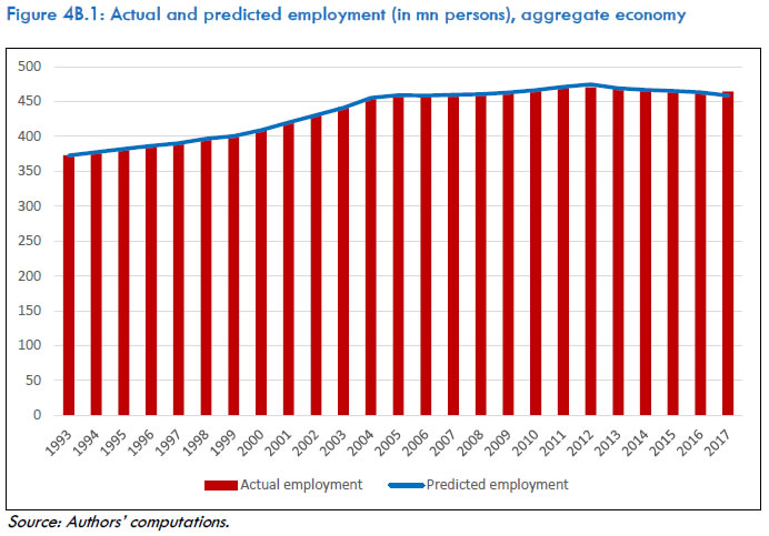 Turning now to the estimates for the four segments of the economy (see Fig. 4B.2), in the industry sector (excluding construction), the average growth rate in real wages was 5.4 percent per annum during 2003-2011 which increased to 8.2 percent per annum during 2012-2017. The fact that there has been a fall in employment in this sector between 2011 and 2017 appears to be explainable mostly by this factor. By contrast, in the agriculture and allied sector, there has been only a moderate increase in the growth rate of real wages, up from 5.1 percent per annum during 2003-2011 to 5.6 percent per annum during 2012-2017. The fall in employment that took place in this sector between 2011 and 2017 thus cannot be attributed only or mostly to increase in the growth rate in real wages. The explanation lies elsewhere too. Another important factor that seems to have played a role is the fall in the growth rate in real GVA – it fell from 3.9 percent per annum during 2003-2011 to 3.1 percent per annum during 2012-2017.79 It is interesting to observe that the fall in aggregate employment in the Indian economy between 2011 and 2017 has been smaller than that predicted by employment estimates generated by the model. According to the model-based estimates, employment should have decreased by about 13 million whereas the actual fall was by about 7 million. The source of this difference lies primarily in the industry sector. Going by the employment estimates based on the estimated model, employment in industry (excluding construction) should have decreased by about 7.2 million between 2011 and 2017 – the actual fall was much lower at 2.4 million. It appears that the negative effect of an acceleration in the growth rate in real wages in manufacturing during 2012-2017 was offset to a considerable extent by certain other developments in the manufacturing sector. 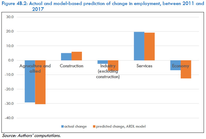 An interesting academic question is if the models were estimated using data up to 2004 (EUS 61st round) and then the model were used to predict employment for 2011 (EUS 68th round) and 2018 (PLFS-I), would the predicted values match the actual, particularly would the prediction be of an increase in aggregate employment between 2004 and 2011 and a fall between 2011 and 2018. This is also a question about checking the robustness of the methodology employed. When this exercise is done, the methodology and the associated predictions are found to be meeting squarely the requirements of robustness. For the period 2004-2011, a fall in employment in agriculture and allied sector and a rise in employment in the other three segments of the economy and at the aggregate level is predicted which tallies with the actual. For the period 2011-2018, a fall in employment in agriculture and allied sector and industry sector (excluding construction) is predicted which tallies with the actual. For construction and services, an increase in employment is predicted for 2011-2017, which tallies with the actual. Figure 4B.3 shows the prediction based on the model estimated using data up to 2011 (called estimate-1) and the prediction based on the model estimated using data up to 2004 (called estimate-2). A comparison is made with actual employment. It is evident that the two sets of predictions are close to each other, and also close to the actual employment. Although the model is estimated using data up to 2004, the prediction for 2011 differs from actual only by 1%, and the prediction for 2017 differs from actual by 0.1%. The analysis presented above has a bearing on an issue concerning the employment series used for the analysis presented in the report. This is the issue of data comparability since in the process of construction of the employment series for the years beyond 2011 the employment estimates based on PLFS have been used in conjunction with the estimates based on EUS 68th round. This issue is taken up for a detailed discussion below. The trends in employment in the 2010s indicated by the PLFS in combination with the EUS 68th round for 2011 are quite different, in several respects, from the trends for the 1990s and 2000s revealed by EUS of 2011 along with that for earlier years. Thus, a fall is seen in aggregate employment between 2011 and 2017, and such a fall has occurred in the agriculture and allied sector and in manufacturing. While a fall in employment in agriculture had occurred also between 2004 and 2011, a fall in employment in manufacturing between successive employment surveys did not occur in the employment estimates of earlier rounds of EUS. The fact that manufacturing achieved a relatively high average annual growth rate in real GVA of about 7.2 percent during 2012-2017 whereas employment in manufacturing decline at the rate of (-)0.7 percent per annum (a fall by about 2.3 million persons) in this period appears puzzling, and contrary to expectations. A negative employment elasticity in manufacturing over a period of seven year has not occurred for Indian manufacturing ever in the period 1980-2011 going by India KLEMS data (perhaps true also for the 1970s, 1960s and 1950s). As regards the fall in employment in agriculture, this is not unrealistic or altogether unexpected, and it should be treated as a mark of the achievements made in terms of structural transformation in the development process in India. While the growth rate of employment in construction during 2012-2017 is positive at 1.6 percent per annum, it has fallen sharply from the growth rate of about 9 percent per annum achieved during 2005-2011. Another interesting difference between the survey findings of PLFS and those of EUS 68th (for 2011) is that the unemployment rate was 2.2 percent in 2011 (previously, 2.3 percent in 1999 and 2.4 percent in 2004) and it was much higher at 6.1 percent in 2017. In several recent studies, the EUS and PLFS data have been combined to analyse the post-2011 trend in employment in India. These include Mehrotra and Parida (2019), Agarwal and Goldar (2020), Ghose and Kumar (2021) and Padhi and Motkuri (2021). In this literature, the issue of comparability of EUS 68th round and PLFS has received attention (see, for example, Jajoria and Jatav, 2020; Padmaja et al., 2020; Mehrotra and Parida, 2019; Padhi and Motkuri, 2021). The general impression that seems to be emerging from the literature is that there is no serious problem of data incomparability in using PLFS data with EUS 68th round data (although, in some articles on this topic, serious concerns have been expressed). It should be noted in this context that in the econometric analysis presented in this annexure, looking into the impact of real wages and real value added on employment, the model estimates predict a fall in employment between 2011 and 2017 in agriculture, industry (excluding construction) and in aggregate economy which is in line with the actual fall as indicated by EUS 68th round and the PLFS. Thus, the econometric results provide some reasons to feel confident about the employment series used for analysis in the Report. In other words, the finding of a fall in aggregate employment and employment in manufacturing between 2011 and 2017 is depicting the reality, and not arising from some issues of data incomparability.80 Based on the studies that have been undertaken on the recent trends in the employment situation in India using PLFS data in conjunction with EUS 68th round data, some key points that emerge may be briefly stated here (some of these points were already noted above in this chapter, but worth repeating here): (1) The rate of unemployment is relatively high (6.1 percent in 2017 and 5.8 percent in 2018). It is still higher among the youth. The rate of unemployment among persons of age 15-29 years was 17.8 percent in 2017 (up from 6.1 percent in 2011). (2) There has been a significant fall in women work participation rate in rural areas, from 37 percent in 2011 to 25.5 percent in 2017. Among women of age 15-29 years in rural areas, the work participation rate has fallen from 41 percent in 2004 to 26 percent in 2011 and then to 14 percent in 2017. (3) The labour force participation rate among youth bore a negative correlation with the economic status of the household in 2011 as revealed by the pattern observed different quintile classes of households according to monthly per capital consumer expenditure (MPCE). This has now changed to a mild positive correlation – the labour force participation rate in the lowest quintile has come down from 48 percent in 2011 to 38 percent in 2017 (Padhi and Motkuri, 2021). This indicates that the youth in rural areas belonging to relatively poorer households is now less inclined and less under compulsion to join labour force than was the situation in 2011. They would rather stay unemployed than take up a low paying low quality job. These facts along with other related facts (such as youth of lower income strata continuing to pursue education in a greater scale) bring out that there has been rationalization of labour in agriculture and this is reflected in the fall in agricultural employment that took place between 2011 and 2017 (also in the period 2004 to 2011). The rationalization of workforce and the removal of surplus labour in agriculture got reflected in the growth in labour productivity and total factor productivity. This, by itself, should not be treated as a matter of serious concern, because in the process of economic development labour is expected to shift from agriculture to more productive jobs in the non-agricultural sector. A much more important point to note regarding the trends in employment in India in the recent period is that the employment in manufacturing has fallen, and thus manufacturing has not been able to absorb the workers that moved out of agriculture. The analysis presented later in Chapter 8 of the Report brings out that the growth rate in employment in the formal segment of manufacturing had fallen from 4.8 percent per annum during 2000-2007 to 1.1 percent per annum during 2008-2017. In the informal segment, the growth rates in employment were 1.6 percent per annum during 2000-2007 and it came down to (-) 0.5 percent per annum during 2008-2017. Evidently, the fall in employment in manufacturing in the recent period is traceable to the failure of the informal manufacturing sector in sufficiently enhancing job opportunities. Chapter 5: Investment and Capital Input 5.1 Introduction Capital is an essential input in the production process, and its importance in understanding the sources of growth is widely acknowledged in the literature. Empirical analysis of sources of economic growth requires pertinent measures of capital input to quantify these sources properly. However, measuring capital is the most complex of all input measurements in productivity and growth analysis. The India KLEMS database, which is primarily aiming to understand sources of growth using a growth accounting framework, provides estimates of capital input at the industry level. These measures are based on the concept of capital services rather than conventional capital stock measures. A measure of capital services is most appropriate from the perspective of productivity analysis, as it helps account for the contribution of capital into production more accurately (Jorgenson, 1963; Jorgenson and Griliches, 1967; Hall and Jorgenson, 1967). This chapter analyses the trends in physical capital in Indian industries during the period 1980-81 (financial year, written as 1980) to 2017-18 (2017). Specifically, we examine the trends in investment/GDP ratio, real investment, capital stock, and growth rates of capital services at the industry level. As in the case of other chapters in this report, all the data used in the analysis are based on India KLEMS dataset version 2019 (hereafter IKD-2019). The analysis in this Chapter will be primarily confined to broad sectors of the economy, while more detailed tables are provided in the annexure. The analysis covers the period 1980-81 to 2017-18, subdivided into three sub-periods, 1980-81 to 1993-94, 1994-95 to 2002-03, and 2003-04 to 2017-18. The methodology used to construct the capital service growth rates is based on Jorgenson (1967) and Christensen and Jorgenson (1969).81 This approach, rooted in neoclassical theory, required detailed asset-wise data on investment, investment prices, rate of return of capital, and the user cost (or rental prices) of capital for the 27 KLEMS industries. While all the final estimates of gross capital formation (referred to as investment throughout this paper) are consistent with the National Accounts Statistics (NAS) with base year 2011-12, several imputations have been made to generate consistent series of capital input for individual industries and assets. For this purpose, we have relied heavily on the annual survey of industries (ASI) for the formal manufacturing sector and National Sample Survey (NSS) for the unorganised manufacturing sector. Moreover, we have obtained detailed asset-industry data on GFCF from NAS, which are not usually published. The aggregate capital services growth rates are measured using estimates of asset-specific capital stocks and user costs (or rental prices) for three individual assets. The three assets considered are construction, machinery, and transport equipment. Rental prices or the user costs of these individual assets are calculated using distinct asset prices and depreciation rates, for each of the 27 KLEMS industries, which includes 13 manufacturing industries and 14 non-manufacturing industries. This basically means that the India KLEMS consists of data on GFCF, investment price deflators, rental prices, and capital stock for three individual assets for all the 27 industries. All this information is combined to produce a measure of aggregate capital service growth rates or the rental weighted growth rates of three individual asset-wise capital stock, which forms the capital input used in the underlying growth accounting exercise in the India KLEMS. The chapter will not discuss the details of the underlying methodology used in calculating capital stock and capital services, nor the construction of basic investment data series. For a detailed explanation of the methodology used in constructing the capital input series in IKD 2019, please refer to the India KLEMS Data Manual. We observe an increasing role of equipment capital (i.e., machinery and transport equipment) in the Indian economy, which helps improve capital composition effects. Capital services growth rates are mostly higher than capital stock growth rates across the board. Much of the recent expansion in capital services and capital deepening is in the market services sector. The chapter is organised in five sections, and the rest of it is structured as follows. In the second section, we focus on the composition and growth in real investment across broad sectors of the economy. We discuss the distribution of investment in the Indian economy across sectors by two broadly-defined asset categories—equipment and non-equipment, and trends in real investment growth across these two categories. It also documents the investment-to-GDP ratios in different sectors of the economy. Section 5.3 seeks to analyse the changing composition and growth rate of estimated capital stock by broad sectors of the economy over the years. In Section 5.4, we discuss the capital service growth rates, along with the contribution of equipment and non-equipment assets to capital service growth rates in each of the broad sectors of the economy. Section 5.5 looks at the composition effects, where we compare the growth rates of capital stock with that of capital services. The final section concludes. 5.2 Composition and Growth of Investment In this section we examine the changes in the composition of investment across sectors and assets, along with the growth rate of real investment. Detailed industry tables are provided in the annexure. 5.2.1 Distribution of Investment across Broad Sectors Figures 5.1 and 5.2 depict the distribution of total gross fixed capital formation, along with equipment and non-equipment assets (throughout this report, non-equipment refers to building and construction assets) across the seven broad sectors of the economy. Among these, the non-market services sector constituted the highest share in aggregate investment in the Indian economy, on average, for the entire period, followed by market services. Together, these two sectors, which constitute the economy's service sector, comprised at least half of the total investment in the economy across the three time periods we have chosen. Manufacturing came third, except for the period 1994-95 to 2002-03, during which it had a slightly higher share than market services. This was likely a reflection of the post-reform investment uptick in the manufacturing sector. 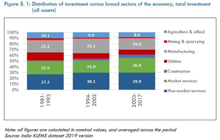 The manufacturing sector registered the biggest improvement in investment share in the 1990s, followed by non-market services and construction. All other sectors dropped their shares. However, in the post-2000 period, manufacturing share dropped substantially by more than 5 per cent, which was almost entirely offset by market services. Other sectors that lost shares include utilities, agriculture, and non-market services, whereas construction share improved. 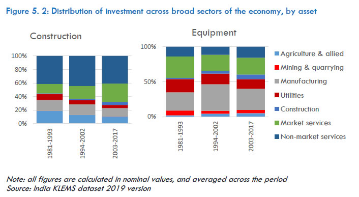 There are, however, compositional differences among sectors regarding their relative share in aggregate investment. The manufacturing sector maintained an edge over other sectors in terms of equipment investment in the 1990s and 2000s. Industries in the market services sector and utility industry are the others that had high equipment share, whereas agriculture, mining, and construction industries contributed relatively less. In the case of non-equipment, however, non-market services constituted the highest portion of the investment. For instance, non-market services occupy more than 40 per cent of all construction investment in the economy. Although manufacturing had about 16 per cent in the 1980s and 1990s, its share fell to 12 per cent in the 2000s, which was somewhat captured by market services that improved from 14 per cent in the 1980s to 27 per cent in the 2000s. Agriculture nearly halved its relative presence in construction investment from 19 per cent in the 1980s to 10 per cent in the 2000s. 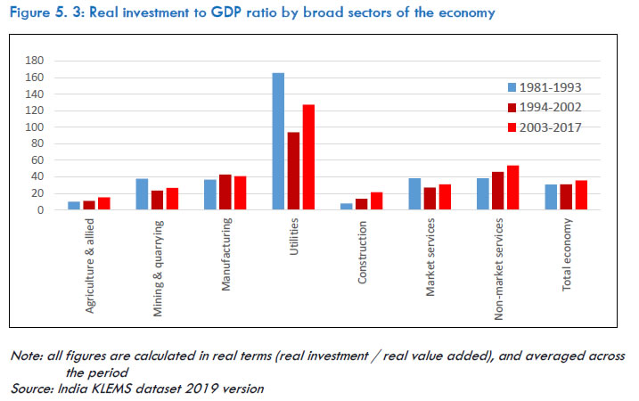 However, the investment to GDP ratio measured in real terms was the highest in the utility industry, which is not unexpected, given the high capital intensity in the energy sector (Figure 5.3). Among the other sectors, the highest investment to GDP ratio was in the non-market services, which includes the government sector. Agriculture and construction industries had the lowest investment intensity. This pattern holds across the three time periods. However, investment intensity increased in all the sectors in the 2000s compared with the 1990s, except manufacturing. The highest increase in the non-utility sectors was in construction, followed by non-market services. Agriculture also saw an increase, in fact, a consistent increase from the 1980s to the 1990s and further in the 2000s. On the other hand, the investment/GDP ratio in manufacturing, after a remarkable rise in the 1990s, dropped marginally in the 2000s. In fact, in the 1990s, investment intensity fell substantially in mining, utilities, and market services. Simultaneously, it improved in manufacturing, non-market services, and construction, leading to a nearly stable overall investment/GDP ratio. In the 2000s, with the substantial increase in the utilities and most sectors except for manufacturing, the overall investment intensity improved. 5.2.2 Growth rate of real investment by broad sectors In the India KLEMS database, the capital stock and capital services are constructed using real investment, measured as nominal investment deflated by relevant asset-wise investment deflators. The growth rate of real investment for the broad sectors are plotted in Figures 5.4 to 5.6. These are the growth rates of simple additions of individual industry investments and are not weighted growth rates. Figure 5.4 shows the growth rate of total investment across all assets, and in Figures 5.5 and 5.6, we divide the total investment into equipment and non-equipment assets, respectively. Real investment growth was the highest in the aggregate economy during the 2003-18 period. This was driven by faster growth in equipment investment. During the other two sub-periods, the aggregate investment growth hovered around 5 to 6 per cent, whereas it was about 8 per cent during the 2000s. Aggregate economy real investment growth was 5.3 per cent in the 1980s, when investment grew between 5 and 7 per cent on average in mining, manufacturing, utilities, and services—both market and non-market, whereas it was dismal at 1.3 per cent in agriculture, and moderate at 3.4 in construction. In the 1990s, investment growth improved in the economy, with construction and non-market services, both seeing a rapid rise from the previous period. While manufacturing still registered an impressive 5.5 per cent growth, it was lower than the previous period. In the 2000s, the agriculture sector, which had already improved its growth in the 1990s over the 1980s, further sustained a growth rate above 4.5 per cent. Among the other sectors, mining, construction, and market services grew at a substantial rate, although the construction sector saw an erosion in its growth rate from the previous period. Investment growth in manufacturing improved, registering an 8 per cent growth rate, while it fell in the non-market services sector. 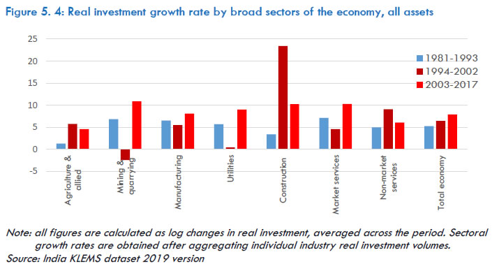 Among the two asset categories, investment in construction grew at about 4 per cent in the economy in the 1980s, which increased to 8.5 per cent in the 1990s. The rise was primarily a result of a massive increase in construction and market services, but other sectors such as agriculture, manufacturing, and non-market services also showed an uptick. While the Indian economy seems to have seen a construction boom in the 1990s, the overall growth rate of construction investment fell to 5.4 per cent in the 2000s. So, while construction investment increased in all sectors in the 2000s, with the highest increase in construction, mining and quarrying, and market services, the rate of increase in most sectors was lower than in the 1990s. While agriculture, manufacturing, and non-market services saw a growth rate of about 3-5 per cent, other sectors had a 7 to 9 per cent growth rate, resulting in overall growth of 5.4 per cent. 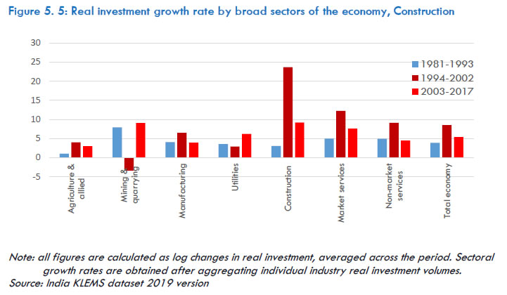 Equipment investment had its best performance in the 2000s compared with the previous periods. While it grew at 8 per cent in the 1980s, its growth performance was very dismal at 2 per cent in the 1990s—mainly on account of market services. The 2000s experienced a significant boost with nearly 12 per cent growth—with equipment investment showing an even higher increase in general, and double-digit growth in most sectors. Agriculture was the only exception. Even there, the growth rate was an impressive 8.5 per cent. Market services were the best performer among all the seven broad sectors in terms of equipment investment growth. 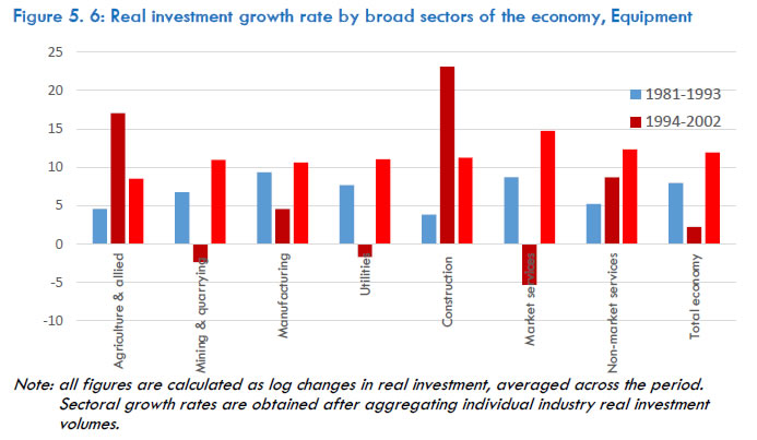 Source: India KLEMS dataset 2019 version 5.3 Composition and growth rates of capital stock Using real investment by different asset types,82 we estimate capital stock for each asset type by industry, using the standard perpetual inventory method. In doing this, we use asset-specific depreciation rates (see the data manual). This section documents the trends in and composition of capital stock across broad sectors of the economy. First, we examine the changes in the composition of capital stock, by looking at the share of equipment and non-equipment assets in total capital stock. Then, we look at the growth rates of capital stock over the three time periods across broad sectors of the economy. 5.3.1 Changing composition of capital stock Figure 5.7 depicts the composition of aggregate capital stock over the last 37 years, which shows a clear shift from non-equipment capital to equipment capital. Yet the overall capital stock in the economy is dominated by construction capital stock. For instance, the share of equipment capital stock increased from 15 per cent in 1980 to 32 per cent in 2017. Indeed, this has resulted in a drop of non-equipment share from 85 per cent to 68 per cent, yet close to 70 per cent of all capital stock in the economy consists of buildings and structures. 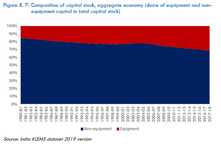 Among the broad sectors of the economy, the highest share of equipment capital in the overall capital stock is in the mining sector (Figure 5.8). Among the non-mining sectors, manufacturing, utilities, and construction sectors maintain dominance over other sectors, and non-market services and agriculture are the ones with the lowest equipment capital stock among the broad sectors. The share of equipment in total capital stock increased over the years in all sectors of the economy, except for market services where it declined. The overall manufacturing sector clearly shows an increase in equipment share but a closer look at the disaggregated industry level suggests that the high equipment share is primarily in petroleum, paper, transport equipment, and food products industries (Annexure Table 5A.3). Many industries, such as textiles, non-metallic mineral products, and machinery, have seen a fall in equipment share. 5.3.2 Growth rates of capital stock Figure 5.9 shows the annual growth rate of capital stock in each of the three assets in the aggregate economy, and in Figure 5.10, we have the average growth rate of total capital stock in each broad sector. As shown in Figure 5.9, growth in equipment capital was much more volatile83 compared with non-equipment and aggregate capital stock. In the 1980s through early 2000s, equipment capital grew somewhat stable, but after a drop in 2002-03, it accelerated substantively until the global financial crisis. Ever since then, it started falling, along with the construction capital stock. But again, during 2015-17 it shows more resilience. On the other hand, construction capital increased consistently until the global financial crisis and started falling since then. 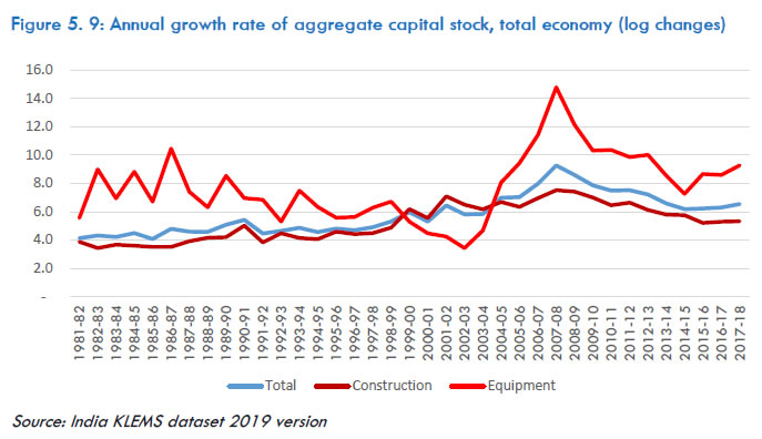 Total capital stock in the aggregate economy grew at around 5 per cent in the first two sub-periods, which accelerated to 7 per cent in the 2000s (see Figure 5.10). Interestingly, in terms of the asset composition, while the growth rate of construction capital stock improved from 4 per cent in the 1980s to 5.3 per cent in the 1990s, equipment stock growth fell from 7.4 per cent to 5.3 per cent, thus both assets registered the same growth rate in the 1990s. The uptick in the total capital stock growth in the 2000s is supported by both assets, although much rapid improvement is seen in the equipment capital stock. 5.4 Capital service growth rates Aggregate capital service growth rates, obtained as weighted growth rates of individual asset-specific capital stock, with user-cost as weights, are provided in Figure 5.13. The user costs were obtained using the methodology developed by Jorgenson (1967) and Christensen and Jorgenson (1969) but deploy an external rate of return.84 The aggregate capital service growth rates in the chart are divided into contributions from equipment assets and non-equipment assets. First, aggregate capital services in the economy have increased from about 5 per cent in the 1980s and 1990s to close to 8 per cent in the 2000s. Second, most of these increases in aggregate economy capital services come from construction and services sectors, with market services dominating the latter. The manufacturing sector has seen somewhat stable growth rate of capital service over the entire period of analysis, although it was relatively better in the 1990s. 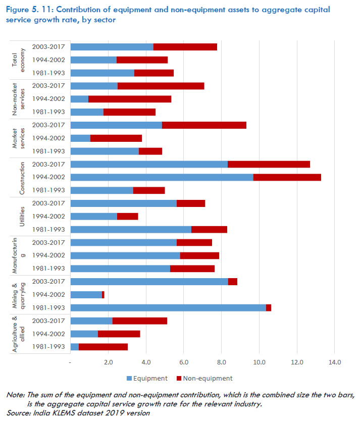 Looking at the contribution of the two asset types—equipment, and non-equipment (construction), in absolute terms, the contribution of construction and building investment fell in the 1990s in agriculture, mining, manufacturing, and utility sectors. At the same time, it improved in the construction and services sectors (both market and non-market service). The volume of increases was much higher than the volume of declines, resulting in an overall improvement in the construction's contribution to capital services growth in the aggregate economy. In the 2000s, the contribution of construction capital to capital service growth rate further increased across the board, except in the manufacturing sector, where it fell marginally. | Table 5.1: Contribution of equipment and non-equipment assets to aggregate capital service growth rate, manufacturing | | | Contribution of Equipment capital | Contribution of non-equipment capital | | | 1981-1993 | 1994-2002 | 2003-2017 | 1981-1993 | 1994-2002 | 2003-2017 | | Food pdts., beverages & tobacco | 3.7 | 3.4 | 4.0 | 3.2 | 3.6 | 3.0 | | Textiles & leather | 6.3 | 5.8 | 3.8 | 2.3 | 3.1 | 3.3 | | Wood & wood pdts. | 2.5 | 2.5 | 1.9 | 3.3 | 7.1 | 2.9 | | Pulp & paper pdts. | 2.5 | 3.4 | 2.3 | 6.8 | 0.4 | 0.2 | | Coke & petroleum pdts. | 14.7 | 17.4 | 9.4 | 1.6 | 0.5 | 0.5 | | Chemicals & chemical pdts. | 3.3 | 6.2 | 5.7 | 0.5 | 1.1 | 1.1 | | Rubber & plastic pdts. | 12.1 | 7.7 | 6.0 | 3.7 | 2.4 | 1.6 | | Non-metallic mineral pdts. | 10.7 | 7.4 | 5.0 | 1.8 | 4.6 | 1.7 | | Basic metals & metal pdts. | 6.8 | 4.3 | 7.2 | 1.3 | 0.8 | 1.4 | | Machinery, nec. | 7.0 | 4.3 | 6.1 | 2.3 | 2.6 | 3.0 | | Electrical & optical eqpt. | 5.7 | 6.9 | 3.9 | 1.0 | 2.3 | 1.8 | | Transport eqpt. | 6.6 | 8.8 | 9.3 | 1.1 | 1.2 | 1.3 | | Other manufacturing | 2.1 | 2.1 | 3.5 | 4.4 | 6.9 | 3.9 | | All manufacturing | 5.3 | 5.8 | 5.6 | 2.4 | 2.1 | 1.9 | Note: The sum of the equipment and non-equipment contribution is the aggregate capital service growth rate for the relevant industry.
Source: India KLEMS dataset 2019 version | The contribution of equipment capital— often argued to have a higher role in boosting economic growth (De Long and Summers, 1991)85 —increased only in agriculture in both periods. Among the other sectors, it fell substantially in mining, utility, and market services, and slightly in non-market services in the 1990s, while it improved in the mining and manufacturing sectors. However, the improvement in manufacturing has been minor and was confined primarily to petroleum, chemicals, electrical & optical equipment, and transport equipment sectors. In all other sectors, it fell (Table 5.1). In the 2000s, construction and manufacturing saw declines in equipment capital service growth rate, while all other broad sectors saw improving contribution from equipment capital. The decline in manufacturing was modest, as the substantial fall in several sectors including petroleum, electrical & optical equipment, and non-metallic minerals, was somewhat offset by improvements in basic metals and machinery sectors (Table 5.1). In relative terms, in the 1980s, more than 80 per cent of the overall capital services growth in the agricultural sector and more than 60 per cent in the non-market services came from investments in new buildings. In the 1990s, although the relative importance of non-equipment capital fell in the agriculture sector, it still contributed more than 60 per cent of the sector's overall capital service growth rate. Simultaneously, the relative contribution of construction assets increased to above 80 per cent in the non-market services. Moreover, market services also joined this group, with almost 3/4th of its overall services coming from construction assets. The high relative contribution of construction in these three sectors led to more than half of the overall capital service growth in the entire economy being driven by construction investment accumulation. However, in the 2000s, construction investment's relative importance fell across the board except in the construction sector. Yet, the non-market services and agriculture maintained relatively high contributions from investment in buildings—50 to 65 per cent. Interestingly, in the 1980s, 60 per cent of overall capital service growth in the aggregate economy was driven by equipment capital accumulation. This originated primarily from mining, manufacturing, utilities, and construction, where 60 to 90 per cent of capital service growth was from equipment. However, the relative importance of equipment capital fell in the 1990s. Although it improved in the 2000s, it was still less than 60 per cent of the overall capital service growth rate observed in the 1980s. The drop in the 1990s and the improvement in the 2000s were both driven primarily by services. In relative terms, the contribution of equipment capital improved in the agriculture sector the most, from just 14 per cent of overall capital service growth in the 1980s to nearly 40 per cent in the 1990s. At the same time, it improved from 68 per cent to 74 per cent in manufacturing and fell everywhere else, with two services segments of the economy seeing rapid declines. Overall, with a substantial drop in equipment contributions in the market and non-market services, the contribution from equipment in the economy's capital service growth rate dropped to less than half in the 1990s. In the 2000s, however, the contribution of equipment capital relative to non-equipment increased, everywhere except in construction, with considerable improvement in utilities and services and marginal in other sectors. In the construction sector, the absolute contribution of equipment capital growth fell from 9.7 per cent to 8.3 per cent, while that of construction improved from 3.6 per cent to 4.4 per cent, thus lowering its relative importance and leading to a fall in the overall capital service growth in the sector. 5.5 Capital composition effects This section looks at the difference between the growth rates of conventional capital stock measures and our measures of capital services. This difference is often considered an indicator of the quality of capital, as it is a direct function of the change in capital composition towards higher quality equipment (Jorgenson, 2001). For instance, increasing the share of ICT equipment in the total capital increases the overall quality of capital, as they have relatively high marginal products. In this paper, following Harper et al. (1989), we call it a ‘composition effect’, as it is primarily a result of accounting for asset composition changes. | Table 5.2: Capital composition effects, by industry | | | 1981-1993 | 1994-2002 | 2003-2017 | | Agriculture & allied | 0.13 | 0.67 | 0.69 | | Mining & quarrying | 0.08 | -0.11 | -0.03 | | Food pdts., beverages & tobacco | 0.56 | 0.06 | 0.56 | | Textiles & leather | 0.04 | -0.56 | -0.37 | | Wood & wood pdts. | 0.48 | -0.57 | 0.40 | | Pulp & paper pdts. | 0.12 | 1.86 | 0.94 | | Coke & petroleum pdts. | -0.42 | 1.17 | 0.05 | | Chemicals & chemical pdts. | 0.20 | 0.02 | 0.23 | | Rubber & plastic pdts. | 0.65 | 0.28 | 0.43 | | Non-metallic mineral pdts. | 1.02 | -2.19 | 0.63 | | Basic metals & metal pdts. | 0.29 | 0.11 | 0.35 | | Machinery, nec. | 0.09 | -0.63 | 0.44 | | Electrical & optical eqpt. | 0.79 | -0.23 | -0.12 | | Transport eqpt. | 0.73 | 0.79 | 0.40 | | Other manufacturing | 0.02 | -0.32 | 1.02 | | Utilities | 1.07 | 0.03 | 0.68 | | Construction | -0.56 | 0.46 | 0.06 | | Trade | -0.89 | 0.63 | 0.48 | | Hotels & restaurants | 0.69 | -0.26 | -0.65 | | Transport & Storage | 0.77 | -1.01 | 0.84 | | Post & telecom | 0.72 | 0.73 | 2.09 | | Financial services | 0.74 | 1.25 | 0.66 | | Business services | 0.06 | 0.26 | 1.12 | | Public administration | 1.22 | -0.29 | -0.10 | | Education | 0.61 | 1.04 | 0.57 | | Health & social work | 0.92 | 1.36 | 0.84 | | Other services | 0.07 | 0.26 | 0.81 | | Total economy | 0.88 | -0.15 | 0.60 | Note: The capital composition effect is the difference between capital service growth rate and capital stock growth rate.
Source: India KLEMS dataset 2019 version | Capital stock and capital service growth rates for the 27 industries are given in the annexure Tables 5A.5 and 5A.6. The results suggest an acceleration in capital service growth rates over the three time periods in the aggregate economy and more than half of the industries. Table 5.2 provides the capital composition effects for three time periods, for each of the 27 industries and the aggregate economy. Faster growth in capital services compared with capital stock would indicate a positive composition effect, while the opposite would suggest a negative composition effect. Interestingly, the overall composition effect was high in the 1980-93 period, while it was negative in the 1990s, and turned positive again in the 2000s. These aggregate pictures, however, are reflections of wide-spread positive composition effect across sectors in the 1980s and 2000s, while the negative effects in the 1990s were mainly emanating from a few sectors. In the 1980s, out of the 27 sectors, 22 showed a higher capital service growth rate than capital stock growth. Among those with negative composition-effects are sectors, trade, construction, and petroleum. However, they registered a positive composition effect in the 1990s, despite many more sectors showing negative composition effect during this period. Only 17 of the 27 sectors had a positive composition effect in the 1990s, while many sectors, including non-metallic minerals, transport services, machinery, and public administration, had a negative effect. The aggregate economy-wide composition effect was also negative during this period, indicating a shift away from high marginal productive assets. In the 2000s, capital services grew faster than capital stock at the aggregate level, indicating a positive composition effect. As in the 1980s, 22 of the 27 sectors had positive composition effect, with the dominant ones being post and telecommunication services, business services, other manufacturing, paper products & publishing, and transport services. On the other extreme, with negative composition effects, were hotels and restaurants, textiles, electric and optical equipment, and public administration. 5.6 Summary and conclusions The role of capital in economic growth is widely acknowledged in the economic growth literature. However, capital remains one of the most challenging concepts when it comes to measurement. Barring several controversies around the measurement of aggregate capital for understanding the contribution of factor inputs and productivity to economic growth (for instance, see Cohen, and Harcourt, 2003 for a review of the famous Cambridge Controversy), many economists now use capital stock and capital services to understand sources of growth. From a productivity and sources of growth perspective, what is quite important is to know how much of the services of capital—just as in the case of labour—has been used in the production process so that it can be accounted for accurately. This has led to a wider consensus that an appropriate measure of capital input in the productivity analysis is capital services, commonly measured as a weighted index of asset-wise capital stocks, with each asset being adjusted for its marginal productivity (Schreyer et al, 2003). This paper documents the trends in capital stock and capital services for 27 industries, available in the India KLEMS database. The chapter starts with examining the trends in investment and then analyses trends in capital stock, capital services, and capital composition effects. The chapter is largely descriptive in nature but opens several avenues for further analytical research. We observe that the aggregate investment growth has improved over the three-time periods we have considered—1980-81 to 1993-94, 1994-95 to 2002-03, and 2003-04 to 2017-18, with the fastest growth being registered in the 2000s. Construction and market services sectors were the two main drivers of the high growth in the 2000s, but all other broad sectors of the economy, including manufacturing, also grew faster in the 2000s. A rapid increase in equipment investment facilitated the faster growth in the total investment in the 2000s, the growth rate of which accelerated substantially across the board, while that of non-equipment investment growth eased compared with the previous period. In context of capital stock and capital services, we observe that, in general, the composition of capital stock is moving towards an increased share of equipment capital in the overall economy. However, there are differences across sectors. For instance, non-market services and agriculture sectors, despite seeing a consistent increase in the equipment share, maintain a relatively low presence of equipment capital compared with manufacturing construction and market services. The general rise in the share of equipment capital also leads to a positive capital composition effect, resulting in a relatively higher capital service growth rate compared to the capital stock growth rate. Overall, the aggregate capital services in the economy have increased from about 5 per cent in the 1980s and 1990s to close to 8 per cent in the 2000s. Annexure 5A: Additional Tables | Table 5A.1: Distribution of total investment across industries | | | 1981-1993 | 1994-2002 | 2003-2017 | | Agriculture, hunting, forestry & fishing | 10.1 | 9.0 | 8.0 | | Mining & quarrying | 3.7 | 2.0 | 2.2 | | Food products, beverages & tobacco products | 2.7 | 3.1 | 2.5 | | Textiles, textile products, leather & footwear | 2.4 | 3.4 | 2.7 | | Wood & products of wood | 0.2 | 0.3 | 0.2 | | Pulp, paper, paper products, printing & publishing | 3.2 | 1.5 | 0.7 | | Coke, refined petroleum products & nuclear fuel | 0.7 | 1.6 | 1.5 | | Chemicals & chemical products | 2.6 | 3.5 | 2.1 | | Rubber & plastic products | 0.7 | 1.1 | 0.7 | | Other non-metallic mineral products | 1.1 | 2.1 | 1.4 | | Basic metals & fabricated metal products | 4.2 | 3.8 | 3.9 | | Machinery, nec. | 1.0 | 1.0 | 1.1 | | Electrical & optical equipment | 0.9 | 1.3 | 0.9 | | Transport equipment | 1.0 | 1.5 | 1.6 | | Manufacturing, nec; recycling | 0.5 | 0.8 | 0.6 | | Electricity, gas & water supply | 14.0 | 10.0 | 8.7 | | Construction | 1.5 | 2.8 | 5.3 | | Trade | 1.2 | 1.4 | 4.9 | | Hotels & restaurants | 0.5 | 0.4 | 0.8 | | Transport & Storage | 17.3 | 9.7 | 7.0 | | Post & telecommunication | 1.1 | 1.8 | 2.2 | | Financial services | 1.6 | 3.0 | 1.5 | | Business services | 0.9 | 4.8 | 9.5 | | Public administration & defense; compulsory social security | 12.5 | 8.4 | 9.1 | | Education | 0.4 | 0.8 | 1.8 | | Health & social work | 0.3 | 0.5 | 1.1 | | Other services | 13.9 | 20.4 | 17.9 | | Total economy | 100.0 | 100.0 | 100.0 | | Source: India KLEMS dataset 2019 version |
| Table 5A.2: Real investment/GDP ratio by industry | | | 1981-1993 | 1994-2002 | 2003-2017 | | Agriculture, hunting, forestry & fishing | 9.6 | 9.7 | 14.9 | | Mining & quarrying | 14.9 | 8.9 | 20.6 | | Food products, beverages & tobacco products | 36.5 | 41.7 | 44.0 | | Textiles, textile products, leather & footwear | 29.3 | 47.2 | 49.0 | | Wood & products of wood | 4.3 | 17.2 | 22.1 | | Pulp, paper, paper products, printing & publishing | 167.0 | 85.6 | 57.5 | | Coke, refined petroleum products & nuclear fuel | 12.0 | 24.3 | 28.5 | | Chemicals & chemical products | 31.4 | 32.7 | 29.2 | | Rubber & plastic products | 52.3 | 60.3 | 51.9 | | Other non-metallic mineral products | 25.4 | 50.4 | 43.3 | | Basic metals & fabricated metal products | 33.7 | 30.4 | 48.9 | | Machinery, nec. | 23.0 | 27.5 | 35.1 | | Electrical & optical equipment | 52.3 | 70.3 | 37.6 | | Transport equipment | 23.2 | 32.0 | 36.5 | | Manufacturing, nec; recycling | 48.3 | 67.1 | 54.7 | | Electricity, gas & water supply | 174.9 | 102.6 | 133.3 | | Construction | 4.5 | 10.5 | 21.8 | | Trade | 4.3 | 4.5 | 16.3 | | Hotels & restaurants | 16.9 | 11.2 | 25.9 | | Transport & Storage | 93.4 | 55.2 | 49.4 | | Post & telecommunication | 85.0 | 69.4 | 46.8 | | Financial services | 14.9 | 16.7 | 8.5 | | Business services | 19.4 | 48.4 | 53.8 | | Public administration & defense; compulsory social security | 55.0 | 37.7 | 54.6 | | Education | 7.4 | 10.7 | 21.4 | | Health & social work | 11.6 | 17.2 | 29.6 | | Other services | 36.1 | 50.9 | 65.6 | | Total economy | 25.0 | 26.3 | 34.5 | | Source: India KLEMS dataset 2019 version |
| Table 5A.3: Real investment growth rate (log changes) by industry | | | 1981-1993 | 1994-2002 | 2003-2017 | | Agriculture, hunting, forestry & fishing | 1.3 | 5.8 | 4.6 | | Mining & quarrying | 6.8 | -2.4 | 10.9 | | Food products, beverages & tobacco products | 4.4 | 7.8 | 7.2 | | Textiles, textile products, leather & footwear | 7.6 | 5.6 | 6.7 | | Wood & products of wood | 0.3 | 15.5 | -0.6 | | Pulp, paper, paper products, printing & publishing | -0.6 | 1.9 | 1.3 | | Coke, refined petroleum products & nuclear fuel | 14.1 | 15.1 | 12.1 | | Chemicals & chemical products | 9.1 | 2.0 | 10.8 | | Rubber & plastic products | 13.6 | -2.6 | 12.0 | | Other non-metallic mineral products | 11.3 | 13.1 | 4.2 | | Basic metals & fabricated metal products | 8.1 | -1.8 | 6.7 | | Machinery, nec. | 7.1 | 8.3 | 9.0 | | Electrical & optical equipment | 10.7 | 10.0 | 4.2 | | Transport equipment | 10.0 | 5.3 | 13.6 | | Manufacturing, nec; recycling | 4.4 | 8.4 | 10.2 | | Electricity, gas & water supply | 5.7 | 0.4 | 9.0 | | Construction | 3.4 | 23.4 | 10.2 | | Trade | 3.1 | 7.2 | 21.7 | | Hotels & restaurants | 1.4 | 1.8 | 17.5 | | Transport & Storage | 6.7 | -4.8 | 8.0 | | Post & telecommunication | 12.8 | 3.7 | 13.7 | | Financial services | 8.7 | 3.7 | 2.8 | | Business services | 11.6 | 26.8 | 7.7 | | Public administration & defense; compulsory social security | 2.8 | 5.8 | 8.8 | | Education | 7.6 | 15.6 | 14.0 | | Health & social work | 8.4 | 16.1 | 12.6 | | Other services | 6.1 | 10.0 | 3.6 | | Total economy | 5.3 | 6.4 | 7.9 | | Source: India KLEMS dataset 2019 version |
| Table 5A.4: Equipment share in aggregate capital stock, by industry | | (per cent) | | | 1981-1993 | 1994-2002 | 2003-2017 | | Agriculture, hunting, forestry & fishing | 2.5 | 4.7 | 11.2 | | Mining & quarrying | 90.1 | 89.4 | 88.1 | | Food products, beverages & tobacco products | 20.4 | 23.3 | 27.9 | | Textiles, textile products, leather & footwear | 45.0 | 43.4 | 36.4 | | Wood & products of wood | 14.6 | 14.0 | 13.3 | | Pulp, paper, paper products, printing & publishing | 9.2 | 15.3 | 27.9 | | Coke, refined petroleum products & nuclear fuel | 71.5 | 82.3 | 88.1 | | Chemicals & chemical products | 61.0 | 63.6 | 63.4 | | Rubber & plastic products | 46.5 | 50.0 | 53.6 | | Other non-metallic mineral products | 57.0 | 48.6 | 44.1 | | Basic metals & fabricated metal products | 57.3 | 61.6 | 64.1 | | Machinery, nec. | 47.5 | 42.4 | 39.5 | | Electrical & optical equipment | 49.3 | 52.1 | 48.7 | | Transport equipment | 54.9 | 63.3 | 70.9 | | Manufacturing, nec; recycling | 11.0 | 9.8 | 12.5 | | Electricity, gas & water supply | 37.1 | 42.4 | 48.4 | | Construction | 43.1 | 42.8 | 44.3 | | Trade | 12.6 | 12.9 | 16.1 | | Hotels & restaurants | 26.8 | 29.1 | 21.5 | | Transport & Storage | 43.3 | 46.5 | 50.2 | | Post & telecommunication | 22.8 | 29.0 | 49.1 | | Financial services | 12.4 | 17.6 | 24.4 | | Business services | 0.03 | 1.5 | 6.6 | | Public administration & defense; compulsory social security | 21.1 | 20.9 | 22.3 | | Education | 4.6 | 8.8 | 15.4 | | Health & social work | 7.8 | 13.8 | 23.5 | | Other services | 0.5 | 1.5 | 5.8 | | Total economy | 19.1 | 22.8 | 26.6 | | Source: India KLEMS dataset 2019 version |
| Table 5A.5: Growth rates of aggregate capital stock by industry | | | 1981-1993 | 1994-2002 | 2003-2017 | | Agriculture, hunting, forestry & fishing | 2.9 | 3.0 | 4.4 | | Mining & quarrying | 10.6 | 1.9 | 8.9 | | Food products, beverages & tobacco products | 6.3 | 6.9 | 6.5 | | Textiles, textile products, leather & footwear | 8.6 | 9.4 | 7.5 | | Wood & products of wood | 5.3 | 10.1 | 4.4 | | Pulp, paper, paper products, printing & publishing | 9.2 | 1.8 | 1.5 | | Coke, refined petroleum products & nuclear fuel | 16.7 | 16.7 | 9.8 | | Chemicals & chemical products | 3.6 | 7.3 | 6.6 | | Rubber & plastic products | 15.1 | 9.8 | 7.2 | | Other non-metallic mineral products | 11.5 | 14.2 | 6.2 | | Basic metals & fabricated metal products | 7.8 | 5.0 | 8.3 | | Machinery, nec. | 9.2 | 7.6 | 8.7 | | Electrical & optical equipment | 5.9 | 9.4 | 5.9 | | Transport equipment | 7.0 | 9.2 | 10.2 | | Manufacturing, nec; recycling | 6.5 | 9.3 | 6.3 | | Electricity, gas & water supply | 7.2 | 3.5 | 6.5 | | Construction | 5.6 | 12.8 | 12.6 | | Trade | 5.4 | 6.5 | 16.2 | | Hotels & restaurants | 7.3 | 5.2 | 12.7 | | Transport & Storage | 3.6 | 1.5 | 4.9 | | Post & telecommunication | 9.0 | 8.8 | 10.1 | | Financial services | 7.1 | 9.2 | 4.1 | | Business services | 7.8 | 20.0 | 12.5 | | Public administration & defense; compulsory social security | 5.5 | 3.7 | 7.0 | | Education | 6.7 | 9.9 | 13.0 | | Health & social work | 8.2 | 10.7 | 12.6 | | Other services | 3.0 | 6.0 | 5.7 | | Total economy | 4.6 | 5.3 | 7.2 | | Source: India KLEMS dataset 2019 version |
| Table 5A.6: Capital service growth rates by industry | | (percent per annum) | | | 1981-1993 | 1994-2002 | 2003-2017 | | Agriculture, hunting, forestry & fishing | 3.1 | 3.7 | 5.1 | | Mining & quarrying | 10.7 | 1.8 | 8.8 | | Food products, beverages & tobacco products | 6.8 | 7.0 | 7.0 | | Textiles, textile products, leather & footwear | 8.8 | 8.9 | 7.1 | | Wood & products of wood | 6.1 | 9.6 | 4.8 | | Pulp, paper, paper products, printing & publishing | 9.7 | 3.7 | 2.5 | | Coke, refined petroleum products & nuclear fuel | 16.0 | 17.9 | 9.9 | | Chemicals & chemical products | 3.4 | 7.3 | 6.8 | | Rubber & plastic products | 16.5 | 10.1 | 7.6 | | Other non-metallic mineral products | 12.3 | 12.1 | 6.8 | | Basic metals & fabricated metal products | 8.0 | 5.1 | 8.6 | | Machinery, nec. | 9.2 | 6.9 | 9.1 | | Electrical & optical equipment | 6.4 | 9.2 | 5.7 | | Transport equipment | 7.4 | 10.0 | 10.6 | | Manufacturing, nec; recycling | 6.9 | 9.0 | 7.4 | | Electricity, gas & water supply | 8.3 | 3.6 | 7.1 | | Construction | 4.9 | 13.3 | 12.7 | | Trade | 4.3 | 7.1 | 16.7 | | Hotels & restaurants | 8.6 | 4.9 | 12.1 | | Transport & Storage | 4.3 | 0.4 | 5.8 | | Post & telecommunication | 9.3 | 9.6 | 12.1 | | Financial services | 7.8 | 10.4 | 4.8 | | Business services | 7.7 | 20.3 | 13.6 | | Public administration & defense; compulsory social security | 6.9 | 3.4 | 6.9 | | Education | 7.2 | 11.0 | 13.5 | | Health & social work | 9.0 | 12.1 | 13.5 | | Other services | 3.0 | 6.2 | 6.5 | | Total economy | 5.4 | 5.2 | 7.8 | | Source: India KLEMS dataset 2019 version |
| Table 5A.7: Contribution of equipment capital to capital service growth rate by industry | | (Percentage points per annum) | | | 1981-1993 | 1994-2002 | 2003-2017 | | Agriculture, hunting, forestry & fishing | 0.4 | 1.4 | 2.2 | | Mining & quarrying | 10.5 | 1.7 | 8.3 | | Food products, beverages & tobacco products | 3.6 | 3.4 | 4.0 | | Textiles, textile products, leather & footwear | 6.5 | 5.8 | 3.8 | | Wood & products of wood | 2.6 | 2.5 | 1.9 | | Pulp, paper, paper products, printing & publishing | 2.6 | 3.4 | 2.3 | | Coke, refined petroleum products & nuclear fuel | 14.5 | 17.4 | 9.4 | | Chemicals & chemical products | 3.0 | 6.2 | 5.7 | | Rubber & plastic products | 12.7 | 7.7 | 6.0 | | Other non-metallic mineral products | 10.5 | 7.4 | 5.0 | | Basic metals & fabricated metal products | 6.7 | 4.3 | 7.2 | | Machinery, nec. | 6.9 | 4.3 | 6.1 | | Electrical & optical equipment | 5.4 | 6.9 | 3.9 | | Transport equipment | 6.3 | 8.8 | 9.3 | | Manufacturing, nec; recycling | 2.2 | 2.1 | 3.5 | | Electricity, gas & water supply | 6.4 | 2.5 | 5.6 | | Construction | 3.2 | 9.7 | 8.3 | | Trade | 0.4 | 3.0 | 5.9 | | Hotels & restaurants | 5.5 | 2.5 | 3.9 | | Transport & Storage | 3.8 | -0.1 | 4.8 | | Post & telecommunication | 5.4 | 5.9 | 10.8 | | Financial services | 3.5 | 5.4 | 3.1 | | Business services | 0.1 | 1.3 | 3.4 | | Public administration & defense; compulsory social security | 4.4 | 1.3 | 2.7 | | Education | 1.8 | 3.8 | 4.8 | | Health & social work | 3.1 | 5.6 | 6.6 | | Other services | 0.1 | 0.6 | 2.1 | | Total economy | 3.3 | 2.4 | 4.4 | Note: The numbers in the table are the contribution of equipment capital to the total capital service growth rate in a given industry. The sum of equipment and non-equipment capital contributions add up to the total capital service growth rate for the given industry.
Source: India KLEMS dataset 2019 version | Chapter 6: Trends and drivers of labour productivity in Indian industries 6.1 Introduction India’s pattern of economic growth and subsequent structural changes during different policy regimes has been summarised in many studies (e.g., Krishna, 2015; Jha, 2015, Krishna, et al., 2017, Erumban, et. al., 2019). The GDP growth rate has been quite remarkable during the period 2001-2011 at 7.9 per cent as compared with 5.6 per cent during the earlier decade of 1991-2001 (Krishna, 2015). The acceleration of growth in the past two decades-1991-2011 has been attributed to, among others, substantial policy changes initiated in the early 1990s and that continued through the 2000s. The period of 2001-11 has been defined as period of service-led growth in India by some economists (Ghose, 2015; Das, et al, 2015), as the industrial sector grew at 7.8 per cent whereas services registered an impressive annual average growth of 9.4 per cent. Consequently, this resulted in a structural transformation marked by a larger share of services sector in the overall GDP, and the several aspects of this structural transformation has been analysed in the literature (Kochhar et al, 2006; Islam, 2008; Papola and Sahu, 2012; Krishna, 2015; Chandrasekhar, 2015; Erumban et al., 2015, Krishna, et al., 2017). The primary sector’s share in GDP86 has declined to just 17.9 per cent in 2017-18 (at 2011-12 prices) from 38.5 per cent in 1990-91. The share of the services sector, on the other hand, has increased from 37.6 per cent to 53.9 per cent and the share of the secondary sector just increased from 24 per cent to 28.2 per cent, with the share of manufacturing increasing from 14.9 per cent to 18 per cent. Agriculture contributes only 15 per cent to GDP in 2017 and still employs 42 per cent of the workforce. This structural transformation has thus been from the primary to the tertiary sector, having bypassed the secondary sector. Simultaneously, there has also been a structural shift of the labour force from primary sector (where its share of employment declined from 64.6 per cent in 1990-91 to 42.3 per cent in 2017-18), to services (where the employment share increased from 20 per cent to 33.8 per cent during the same period). This kind of duality cannot happen unless there is a simultaneous structural change happening in the sphere of labour productivity. Such a structural change is part of the economic development process of developing economies that are characterised by large productivity gaps among their different sectors and industries. An economy’s overall productivity depends not only on what’s happening within industries, but also on the reallocation of resources across sectors. So, the structural change in labour productivity at the economy level will take place whenever there is reallocation of labour from low-productivity to high-productivity sectors. Measuring labour productivity is important—as the time profile of labour productivity not only reflects how productively labour is used to generate output but also the personal capacities of persons employed or the intensity of their effort. According to OECD (2008) ‘labour productivity is a revealing indicator of several economic indicators as it offers a dynamic measure of economic growth, competitiveness, and living standards within an economy’. It is in this context that the chapter has examined India’s labour productivity growth at the industry level to understand the proximate sources of growth in the Indian economy for the period 1980-2017. We compute and analyse the estimates of labour productivity (LP) growth for each of the 27 industries, using the India KLEMS database. The chapter is organised as follows: in Section 6.2 we briefly discuss the literature on labour productivity and the methodology and dataset in Section 6.3. Section 6.4 looks at trends in labour productivity for the 27 industries. Analysis of sources of labour productivity and the ‘virtuous’ pattern of growth is carried out in Section 6.5 and Section 6.6 analyses the results for the broad sectors of the economy and the sectoral decomposition for disaggregated industries. A cross-country comparison of labour productivity is covered in Section 6.7 and the last section 6.8 offers a conclusion. 6.2: Literature on Labour Productivity APO (2018) considers labour productivity and its drivers important because of the close links to GDP per capita. Productivity accurately measures the performance of an economy, an industry and a firm in terms of the quantity and the efficiency with which inputs, especially labour, are used to produce goods and services. The efficiency of labour, through its impact on unit cost of production, would also have bearing on the competitiveness of the economy and on its participation in global supply chains. The importance of labour productivity is also emphasised by Krugman (1994), who said that ‘Productivity isn’t everything, but in the long run it is almost everything’. The writings earlier by OECD (2016) and later by Dieppe(ed.2020) has brought labour productivity in focus once again. According to Dieppe (ed. 2020), the experience of the emerging market and developing economies (EMDEs) reveals that growth in labour productivity (LP) also helps in reducing poverty through its impact on the long-term growth in per capita income. The report shows (Fig 1, p.i5) that countries with faster labour productivity growth during 1981-2015, are also the ones which succeeded in reducing their extreme poverty at a quicker pace. Dieppe (ed. 2020) also observes that any external shock, e.g., the global financial crisis (GFC) or Covid 19,87 is likely to have serious impact on labour productivity, resulting in loss in per capita income and increase in poverty and larger is the impact with more severe downturns. Surges or declines in labour productivity generally follow cyclical upswings and declines in GDP and can be persistent if the countries have weak fiscal positions and necessary safeguards are not taken to protect labour. Labour productivity is, however, a partial measure of productivity and reflects the joint influence of a host of factors depending on the growth accounting framework being considered. In a gross output framework, the contribution to labour productivity growth comes from four sources: namely capital deepening with more or better capital (technology); labour quality, or changes in the composition of labour, which comes from investment in human capital; contribution of intermediate input deepening which reflects the impact of more intermediate-intensive production on labour productivity; and finally from TFP growth which contributes to labour productivity point-for point (Jorgenson, 2005; p299). However, in a gross value-added framework there are only three contributors to labour productivity growth; namely - changes in labour composition or labour quality, contribution of capital service per person employed or capital intensity, and total factor productivity (TFP) growth. Based on global productivity trends, Dieppe and Kindberg-Hanlon (2020, p. 316) also find that the drivers of labour productivity growth are “capital-deepening (growth of capital per unit of labour input) or technological and organisational changes, including the adoption of more efficient methods of production, in some cases through capital investment (Hulten, 1992)”. The report also finds that ‘technological’ drivers of productivity explain a large percentage of the variation in labour productivity during 1980-2018 and the technological improvements during the period were responsible for the decline in employment by 70 per cent in the EMDE countries and 90 per cent in the advanced economies. The largest negative effects on employment occurred in those industries, which tended to be more amenable to labour-saving innovation than other industries. International experience indicates that labour productivity of an economy also increases due to reallocation of labour from low-productivity sectors/industries to high-productivity sectors/industries, and Dieppe and Kindberg-Hanlon (2020, p.i8) notes that “labour reallocation towards higher-productive sectors has historically accounted for about two-fifths of overall productivity growth in EMDEs”. They observe that shocks such as the global financial crisis and Covid-19 pandemic may weaken the mechanism of structural change by restricting the mobility of people, thereby slowing the geographical and sectoral labour reallocation. Labour productivity reflects the volume of output produced per unit of labour input (OECD, 2016) and is described as one of the key indicators of economic performance and as an essential driver of change in living standards. It however, also depends on the use of other inputs, such as capital—both physical and intangible; and technical and organisational change. OECD defines labour productivity as GDP per hour worked88 and its growth is measured in GDP at constant prices in the national currency of the country. Dieppe (ed. 2020) also pointed out that GDP per hour worked may be a better proposition to measure labour productivity, but for international comparisons, found it convenient to use output per worker because of wider availability of data for workers than hours. He, however, mentions doing this has the disadvantages of ‘failure to account for the quality and intensity of labour input (pp. 15, Box 1)’. Though labour input may be preferably measured in terms of hours worked, in the case of India, the data on hours worked are either not available or are of low quality and hence labour input is measured in terms of the number of persons.89 6.3. Methodology and Dataset In this section, we discuss the methodology for computing labour productivity in the 27 individual industries in Indian economy. We find the trend in labour productivity over the period 1980-2017 and estimate its sources of growth. We also use the decomposition method (Fabricant, 1942) to find the within-industry productivity growth component and the between-industry component to understand the reallocation or structural change between the industries. In the present chapter, labour productivity is defined as real gross value added per unit of person employed. From the growth accounting framework, we find that there is a strong and direct relationship of labour productivity growth with growth in total factor productivity (TFP). It is because growth in output basically depends on the growth in inputs and the efficiency with which these inputs are used, known as TFP and the inputs used are not only labour and capital but also intermediate inputs. However, the gross value-added version is used and labour productivity, its sources and the decomposition are all based on the value added90 concept following OECD. 6.3.1 Measurement of labour productivity While at the industry level ‘i’, labour productivity (LP) is obtained directly by taking the ratio of real GVA (Vi) to employment (Li), for the broad sectors it may be obtained as the sum of real GVA divided by the sum of employment for all the industries in the broad sector. Thus, where LPi and LPs are labour productivity in the ith industry and the sth broad sector; Vi and Li are the real gross value added and employment for the ith industry and s is the number of industries in a broad sector. However, labour productivity growth is computed simply by the difference of growth rate of value added and growth rate of persons employed by UPSS. It may be mentioned that although labour productivity is a partial productivity measure, it is closely related to wages and, hence, to living standards (Murray, 2016).91 6.3.2 Sources of Labour productivity growth The sources of labour productivity growth are therefore change in capital intensity, change in labour composition, change in intermediate inputs and TFP growth, as shown in (6.3). However, as mentioned earlier, in a gross value-added framework, which is used in the current chapter, the only contributors to labour productivity growth are three; namely - changes in labour composition, contribution of capital service per person employed or capital intensity, and TFP growth, and the growth accounting equation then is:  Dieppe, et.al. (2020, p17, Box 1) however, points out to the limitation in the measurement of both output and inputs (K and L). He argues that “Capital services is a measure of the total physical capital available for production without necessarily considering how much of the existing capital is used actively in the production process (capital utilisation). Similarly, labour input, even if it is finely measured as total working hours, does not account for variable labour effort. This may lead to an overly cyclical measure of productivity.” In such a situation, TFP, which is a measure of residual does not only estimate technological change but also any error in the measurement of capital and labour. The neglect to measure and include ‘natural capital’ as an input is also likely to over-estimate the TFP growth effect. According to Dieppe, et.al. (2020, p18), the measurement of new IT products and changes in the quality of ICT has not been accurately done in many national accounts. However, based on many studies on the impact of mismeasurement on the slowdown in productivity after the GFC, the author concludes (p.19) that “despite some evidence for mismeasurement it is unlikely that a significant part of the broad-based slowdown in productivity growth since the global financial crisis can be explained by it alone (Cerra and Saxena 2017; Syverson 2016).” 6.3.3 Decomposition of labour productivity- within and between effects In this section we study the contribution of the structural change to growth in aggregate labour productivity for the 27 sectors of the Indian economy for the period 1980 to 2017. We use decomposition methods to understand the contributions of structural change to growth in aggregate factor productivity. The decomposition method applied for this purpose can be traced to the methodology in the study undertaken by Baily, Hulten, and Campbell (1992) in the context of manufacturing plants and which was subsequently modified by Haltiwanger (1997). The same decomposition method is now widely used to decompose the growth rate of aggregate factor productivity growth in to a ‘within’ industry productivity growth component and a ‘between’ effect, also known as reallocation effect. It is the ‘between effect’ which is used as a measure of structural change by various researchers (e.g., Ghani, 2013; Goldar and Aggarwal, 2015; Goldar, et al., 2017). The same method is applied for reallocation of labour input in the present paper and is discussed below. The equation 6.5 is similar to equation 6.2, except while equation 6.5 defines labour productivity at the aggregate level of an economy, 6.2 defines it at the sector level. Using the decomposition methodology used by Goldar et al. (2017), the annual change in labour productivity levels is then decomposed into within-industry productivity change and a reallocation effect:  The first term in equation 6.6 is the within industry effect, or the effect of productivity change within each industry. It denotes for each industry, the sum of change in productivity levels weighted by its respective employment share in the previous period. The second term is between industry effect—a measure of worker reallocation across industries—and is calculated by a change in employment weighted by levels of productivity in the previous period. If it is positive, it suggests that workers move to sectors with above-average productivity levels, and this term is often considered as a static reallocation (or between) effect and is also described as the structural change term measuring the movement of workers from low-productivity to high-productivity industries. The last term in the equation is an interaction of change in employment share and change in productivity, and thus it measures the combined effect of changes in employment shares and sectoral productivity in a given period – a co-variance or dynamic reallocation term (Ghani, 2013; Erumban, et.al., 2015). A positive dynamic reallocation term would suggest that the factor input is moving to sectors that see positive productivity growth. We obtain the decomposition of labour productivity growth rates by dividing both sides of equation 6.6 by aggregate labour productivity in the previous period. 6.3.4 Data and variables The source of data used in the current chapter is India KLEMS database, 2019 version.94 The data covers the period 1980-2017, and all the growth rates analysed in the study are calculated for three sub-periods during this period, 1981-93, 1994-2002, 2003-17, with the last sub-period splitting further into pre-and post-global financial crisis, i.e., 2003-07 and 2008-17. All data in India KLEMS refers to the financial year, as with national accounts data. However, the periods in this report will be expressed in terms of the calendar year. For instance, the period 1980-2017 refers to 1980-81 to 2017-18 and financial year 1980-81 is expressed as 1980. 6.4: Labour Productivity – Trends and behaviour In this section we first explain the behaviour of labour productivity growth in the 27 KLEMS industries in section 6.4.1 followed by a discussion about the changes in the growth rates of labour productivity in section 6.4.2. 6.4.1 Labour Productivity growth in the disaggregate industries Trends in growth of labour productivity for 27 industries that constitute the KLEMS framework are presented in Table 6.1 and Figure 6.1. It is evident that the agriculture sector observed a consistent growth of around 2 per cent in labour productivity till 2002 and thereafter, a surge between 2003 and 2017, mainly because of deceleration in growth in employment. As both the level of and growth in employment declined at an average annual rate of 2 per cent during 2008-17, labour moved out from agriculture to other labour-intensive industries95 with similar skill requirements, mainly construction, which experienced an acceleration of 5 per cent in its growth in employment during the same period. Both agriculture and construction not only had and still have similar skill composition, with 65-68 per cent of unskilled labour and only 2.6-3.4 per cent of high-skill labour respectively,96 but both also employ a large proportion of the total employed persons in the economy- 49 and 11 per cent respectively. The other labour-intensive industries are all relatively small in terms of level of employment and do not have much labour absorption capacity. The only other labour-intensive industry with a sizable share in total employment in 2011-12, around 10 per cent, is trade but in 2011, it had only one-third of its employees with low skill and 15 per cent with high skill. Hence, the skill composition and requirement of this industry was different from what was available from the displacement of labour from agriculture. Thus, the trade industry had very limited capacity to absorb the labour that moved out of agriculture and employment in the industry only accelerated at an average annual growth rate of 1.2 per cent during 2008-17. So, while the decline in employment in agriculture boosted its labour productivity, this also led to a decline in the growth in labour productivity of its labour-absorbing industry, namely construction. However, for the overall period of 1981-2017, labour productivity growth in the agriculture sector, although is lower than for the total economy, is still reasonable at 3 per cent per annum. Within the manufacturing sector (comprising 13 industries starting from ‘food products’ at number 3 to ‘manufacturing, nec.; recycling’ at number 15 in Table 6.1) traditional industries such as machinery, nec.; wood and products of wood; pulp & paper; and basic metals and fabricated metal products have low labour productivity. While wood industry is labour intensive, the other industries also employ substantial labour relative to capital and are thus expected to be low in labour productivity. Further, those manufacturing industries, which lately (2008-17) experienced a surge in the growth in labour productivity are textiles, textile products, leather and footwear, wood and products of wood; rubber and plastic products; other non-metallic mineral products; transport equipment; and manufacturing, n.e.c; recycling. Three industries, that are also often clubbed for analysis with the ‘non-manufacturing’ broad sector, are mining and quarrying; electricity, gas and water supply; and construction. A close look at the individual behaviour of these three industries reveals that construction not only has the lowest labour productivity among the three, but also experienced a small negative average growth in labour productivity during 1981-2017. However, the negative growth is restricted only to the first sub-period of 1981-93. Despite remaining a low-productivity sector, the construction sector has boomed in the post-reforms period—with employment growing rapidly. The reasons for low productivity could be the massive deployment of labour in the sector especially after 2004-05 when it absorbed most of the labour displaced from agriculture without any significant improvement in technology. So, growth in the sector’s output could not keep pace with growth in employment. On the other hand, the growth in labour productivity in the electricity industry was quite high at 5.5 per cent during 1981-93 but it subsequently became stagnant and later declined after the 2008 GFC. The mining industry however, consistently experienced an increasing rate of growth in labour productivity in all the sub-periods. One of the main reasons for its relative success is the increase in capital intensity of the industry and the opening of some segments of the industry to the private sector, which would have promoted competition and efficiency. The six industries from number 18 to 23 that are defined as market-services, show much variation among them (Table 6.1). While trade, and post and telecommunication record high growth in labour productivity, the other four industries—hotel, transport, financial services, and business services—display a relatively low growth. The trend in growth in labour productivity in these six industries is also not uniform. While ‘Hotels and Restaurants’, ‘Financial Services’, and ‘Business Services’ show a slower growth after 2002; the other three industries have shown a tendency of faster growth after 2002. In the non-market service sector consisting of four industries (number 24 to 27), variation in labour productivity is not substantive. These industries, except health have grown faster during 2008-17 as a result of gradual reforms in the sector and a fast pace of overall economic growth. Figure 6.1 showing growth in labour productivity over the entire period of 1981-2017 reveals that the top five industries in terms of growth in labour productivity are chemicals, other non-metallic mineral products, public administration, post and telecommunication, and textiles. The five industries that experienced the slowest growth are construction, wood and products of wood, machinery, n.e.c., other services, and transport & storage. Therefore, large differences in levels and growth of labour productivity across the 27 industries are observed. These results are supported by two earlier studies—by Aggarwal (2018) for 27 KLEMS industries and Goldar and Sengupta (2016) for 2-digit organised and unorganised manufacturing industries. Both these studies also find different growth rates of labour productivity in different industries within the same period and across different sub-periods. | Table 6.1: Growth rate of Labour Productivity in 27 industries: 1981-93, 1994-2002, 2003-07, 2008-17 and 1981-2017 | | (per cent per annum) | | S.No. | Industry | Capital intensity | 1981-93 | 1994-2002 | 2003-07 | 2008-17 | 1981-2017 | | 1 | Agriculture, Hunting, Forestry and Fishing | LI | 1.72 | 1.54 | 4.84 | 5.35 | 3.08 | | 2 | Mining and Quarrying | HCI | 2.38 | 4.69 | 5.19 | 5.87 | 4.27 | | 3 | Food Products, Beverages and Tobacco | LCI | 4.86 | 4.83 | 8.89 | 4.81 | 5.38 | | 4 | Textiles, Textile Products, Leather and Footwear | LI | 4.69 | 1.85 | 6.06 | 9.55 | 5.50 | | 5 | Wood and Products of wood | LI | -4.31 | -7.18 | 3.70 | 10.84 | 0.17 | | 6 | Pulp, Paper, Paper products, Printing and Publishing | LCI | 3.65 | -3.59 | 12.20 | 2.95 | 2.85 | | 7 | Coke, Refined Petroleum Products and Nuclear fuel | HCI | 6.81 | 3.92 | 5.18 | 1.65 | 4.49 | | 8 | Chemicals and Chemical Products | HCI | 5.80 | 6.17 | 8.49 | 5.78 | 6.25 | | 9 | Rubber and Plastic Products | LCI | 3.47 | 4.75 | -1.05 | 9.56 | 4.82 | | 10 | Other Non-Metallic Mineral Products | LCI | 5.88 | 5.87 | 2.25 | 9.04 | 6.24 | | 11 | Basic Metals and Fabricated Metal Products | LCI | 1.89 | 4.15 | 7.39 | 2.09 | 3.24 | | 12 | Machinery, nec. | LCI | 2.42 | -1.28 | 8.68 | 2.33 | 2.34 | | 13 | Electrical and Optical Equipment | LCI | 2.37 | 6.37 | 12.47 | 0.01 | 4.07 | | 14 | Transport Equipment | HCI | 1.60 | 6.49 | 5.62 | 8.42 | 5.18 | | 15 | Manufacturing, nec; recycling | LI | 2.34 | 2.01 | 3.72 | 11.26 | 4.86 | | 16 | Electricity, Gas and Water Supply | HCI | 5.54 | 4.45 | 3.83 | 2.24 | 4.15 | | 17 | Construction | LI | -3.08 | 1.24 | 3.47 | 0.45 | -0.19 | | 18 | Trade | LI | 1.19 | 4.35 | 5.89 | 6.97 | 4.16 | | 19 | Hotels and Restaurants | LI | 2.95 | 4.49 | 5.92 | 2.36 | 3.57 | | 20 | Transport and Storage | LCI | 0.97 | 2.13 | 6.31 | 3.94 | 2.78 | | 21 | Post and Telecommunication | HCI | 1.73 | 9.14 | 7.86 | 7.43 | 5.90 | | 22 | Financial Services | LCI | 3.22 | 6.31 | 2.61 | 2.55 | 3.71 | | 23 | Business Service | HCI | 1.64 | 5.48 | 3.82 | 2.29 | 3.04 | | 24 | Public Administration and Defence; Compulsory Social Security | HCI | 3.80 | 6.52 | 6.45 | 7.91 | 5.93 | | 25 | Education | LI | 3.30 | 3.62 | 1.23 | 7.43 | 4.21 | | 26 | Health and Social Work | LI | 5.21 | 3.42 | 6.31 | 5.11 | 4.90 | | 27 | Other services | HCI | 3.22 | 0.71 | 1.20 | 3.97 | 2.54 | | Total | Total economy | | 3.03 | 3.66 | 6.08 | 6.26 | 4.47 | Note: Labour productivity is here defined as real gross value added (at 2011-12 prices) per person employed.
LI stands for labour – intensive, HCI for high capital-intensive, and LCI for low capital-intensive industries.
Source: Authors’ computations from India KLEMS database (2019) |
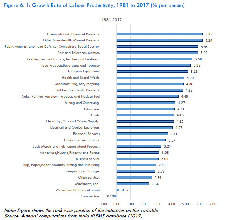 A further investigation of the underlying factors which could explain the differences in the growth of labour productivity is attempted separately for manufacturing industries (Figure 6.2) and the services industries (Figure 6.3). The analysis shows (Figure 6.2) that generally, as expected, the average labour productivity during 1981-2017 in the 13 manufacturing industries has accelerated the fastest in the capital-intensive industries followed by labour-intensive industries and less capital-intensive industries. The same trend is also discernible in the growth in GVA as well as in employment. It indicates that high capital-intensive industries generally observe a fast growth in both GVA and employment as compared with other manufacturing industries. It is, however, observed that growth in labour productivity in the labour-intensive manufacturing industries has not followed a constant trend as it varies between different sub-periods—and it was quite high during the period 2008-17 due to a deceleration of 1.8 per cent per annum in the employment growth during that period. 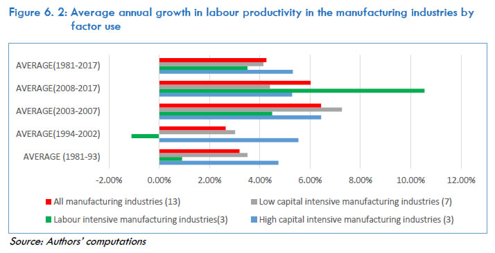 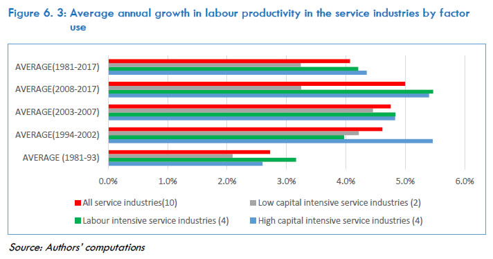 Detailed analysis of the 10 service sector industries (Figure 6.3) empirically indicates that over the entire period of 1981-2017, growth in labour productivity has been the highest in the high capital-intensive service industries, but the difference in the average annual labour productivity growth between these and the labour-intensive service industries s only marginal. The same is true about the growth in GVA and employment, where we observe that the high capital-intensive service industries show higher growth in both GVA and employment, but the growth in labour productivity is almost the same because of the uniform difference in the two growth rates. Inter-temporarily, we do not find a clear trend in the labour productivity growth across service industries with varying capital intensity. The labour-intensive service industries show an impressive acceleration in labour productivity growth during all the sub-periods due to a very high growth in capital intensity in the economy at 6.9 per cent per annum during 2008-17 compared with just 2.5 per cent during 1981-93.97 The growth in labour productivity also accelerated quite fast for the capital-intensive service industries during the sub-periods till 2002, but in 2003-07 these industries experienced a marginal slowdown due to slowing growth in employment from 5.1 per cent during 1994-2002 to 3.4 per cent during 2003-07 and in growth in GVA from 10.6 per cent to 8.2 per cent. Figure 6.4 depicts an analysis of the growth of labour productivity in manufacturing and service industries based on ICT. The 27 KLEMS industries are divided into ICT-producing, ICT-using and non-ICT industries (see Annexure Table 6.A). The figure reveals that (i) during 1981-2017, within the manufacturing industries the non-ICT industries have experienced the highest labour productivity growth due to a low growth in employment, just 2 per cent per annum as compared with 5.2 for ICT-producing and 3.2 per cent for ICT-using manufacturing industries with a quite similar growth in GVA; (ii) in the service industries it is the ICT-producing industries, which show the highest growth in labour productivity due to high growth in both employment and GVA; (iii) the growth in labour productivity in the ICT-using industries has been in between the ICT-producing and non-ICT industries both in manufacturing and service industries; (iv) inter-temporarily there is no clear trend in growth of labour productivity, thus clearly reflecting the uniqueness of each of the manufacturing and the service industries. 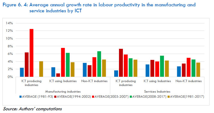 6.4.2 Changes in the growth rate of labour productivity In order to examine the industry level change in labour productivity over time to understand volatility in the growth rates, we consider two sample periods—the period 1994-2007 is taken as the sub-period starting from economic reforms (including the period of high growth) to the beginning of global financial crisis, and 2008-2017 is taken as the sub-period post-global financial crisis (including tapering of high growth). Figure 6.5 ranks the industries in terms of change in productivity growth between these two sub-periods. The industries that experienced a sharp growth in the second period are wood; manufacturing, nec; rubber; textiles; and education. The majority of the industries here is labour intensive in nature. The industries that showed the largest decline are electrical equipment; basic metals; coke & refined petroleum; hotels; and business services. The observed volatility in the growth rate of labour productivity is evident from the sharp increases in the region of 1-14 per cent per annum and the sharp declines ranging between 1 and 9 per cent per annum post-2008. The trend calls for more attention to be paid to the specific sectors to minimise the sharp fluctuation in the growth rates for better planning by the industry. 6.5 Sources of Growth in Labour Productivity and the ‘virtuous’ pattern of growth This section deals with the sources of growth in labour productivity in sub-section 6.5.1 and analysis of the ‘virtuous’ pattern of growth is undertaken in 6.5.2. 6.5.1 Sources of Growth in Labour Productivity The moot question that arises and could help in understanding the underlying trend in the growth of labour productivity is: what are the drivers of labour productivity? This section seeks to address this question. Figure 6.6 captures the contribution of the three sources of growth in labour productivity98—growth in labour quality, capital intensity (capital deepening) and TFP growth for the 27 industries—for the period 1981 to 2017. The figure shows that across the 27 industries, the mean contribution of growth in capital deepening is 3 percentage points out of the mean aggregate labour productivity of 3.98 percentage points; and is followed by just 0.65 percentage points by TFP growth; and only by 0.27 percentage points by growth in labour composition index (or labour quality index). In most of the industries, the contribution of labour composition growth has been quite marginal— less than 10 per cent of its aggregate labour productivity growth (mean being only 7 per cent). It contributes more than 10 per cent to the aggregate labour productivity growth only in the three industries of transport & storage; other services; and health & social work. In 23 out of 27 industries, capital deepening growth contributed the maximum to labour productivity growth, and in the remaining four industries, it is growth in TFP that contributed the maximum to labour productivity growth. These four industries with substantial contribution by TFP growth are manufacturing, n.e.c.; transport & storage; financial services; and public administration. The contribution by TFP growth is negative in eight industries, which does not auger well for the growth of these industries or for the economy. Figure 6.7 reflects the findings of an investigation of the drivers of growth based on ICT use. It reveals that during 1981-2017, the average labour productivity growth rate is the highest in the ICT-producing industries and is the lowest among the non-ICT industries. It also shows that the average contribution of capital deepening is higher than TFP growth and labour quality composition in all the three types of industries—ICT-producing, ICT-using and non-ICT industries. However, while the ICT-producing industries have the highest contribution from TFP growth, capital deepening has the highest contribution in the average growth of labour productivity of the non-ICT industries. Evidently, ICT plays an important role in accelerating the growth of labour productivity and positively impacts TFP growth. Sectorally, capital-deepening growth has contributed substantially to labour productivity growth in all manufacturing industries except manufacturing, n.e.c. In the services sector, it is TFP growth that has done this (with 30 per cent or more contribution) except in trade and business services, where capital deepening has contributed more than 85 per cent of the total growth in labour productivity. In fact, capital deepening has been the primary driver in 23 of the 27 industries. Some reasons for capital deepening in Indian industry99 over the period are (i) reduced cost of capital (Unni, 2015), (ii) relatively low price of capital due to interest subsidies and cheap electricity (Chandrasekhar, 2008), (iii) use of new imported capital intensive technology (Felipe & Hasan, 2006), (iv) market distortions in the form of subsidies to capital and high wages in modern industries (Felipe, 2010), and (v) the emergence and growth of the ‘new service economy’ which is more capital intensive. The adoption of new technology leading to automation and increase in capital intensity of firms and industries, especially in the organised sector in India, is also confirmed by Kapoor (2016), Das et al. (2015) and Goldar (2000). But from a long-term growth prospect, it is necessary that growth in labour productivity is driven more by TFP growth rather than by factor inputs. 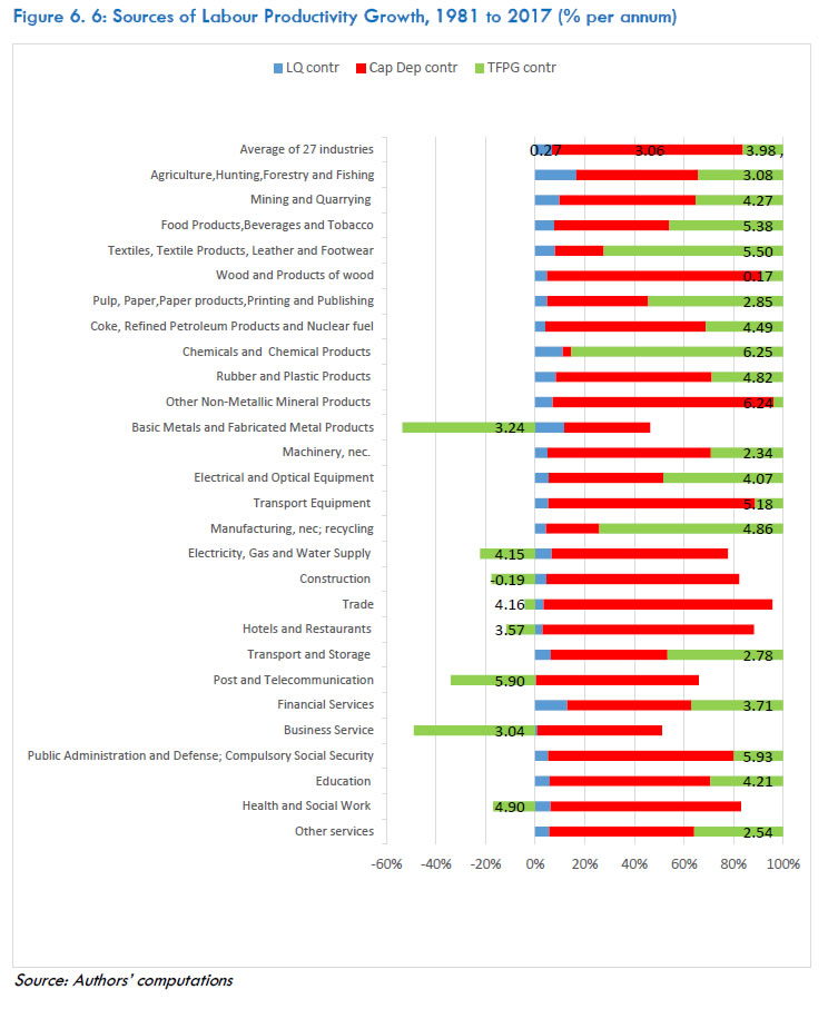 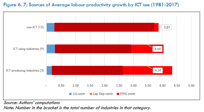 However, the Indian experience is similar to the other Asian countries where capital deepening contributes almost 50 per cent to labour productivity growth and is thus an important engine of labour productivity growth (APO, 2018, pp.78). Dana, et.al. (2020, p.270) has identified some challenges in South Asia including India that are an obstacle to the growth of labour productivity—and these are low rates of female labour force participation, limited integration in global value chains, low R & D development, lack of adequate infrastructure, and the large size of India’s informal sector. Overcoming these obstacles can help in the growth of labour productivity. 6.5.2 The virtuous pattern of growth of labour productivity Once the track record of the 27 industries on their performance on growth in labour productivity is analysed, it is desirable, especially from the policy perspective, to find out which of these industries have followed the ‘virtuous’ path. Mas and Benages (2016) have used two criteria—(i) creating employment, and (ii) achieving growth in labour productivity—to assess if a sector/industry is following a ‘virtuous path’. Figure 6.8 shows there are very few industries in India, which satisfy these two criteria to generate fast growth in employment (above-average growth indicated by vertical blue line) and in productivity (yellow horizontal line) so that these industries could be promoted for creating productive employment. The figure shows that these are the industries of post and telecommunication, rubber and plastic, coke & petroleum, transport equipment, health, manufacturing; n.e.c., and chemical, all of which have experienced higher-than-average labour productivity and employment growth. These industries may be carefully monitored and incentivised to bear the fruits of the virtuous path of high growth in labour productivity and high growth in employment. The industries in other quadrants, especially close to the mean lines, e.g., education, trade, electricity, electrical equipment, food, non-metallic industries, and business services may also be suitably incentivised to move them towards the virtuous path. 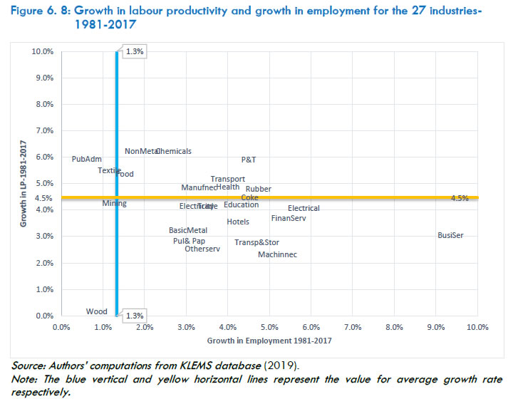 6.6 Labour productivity at the broad sectoral level, reallocation and sectoral decomposition 6.6.1 Level of labour productivity in the broad sectors As the level of labour productivity plays a crucial role in determining the level of earnings and hence the living standard of people, its growth helps in the growth of GDP of an economy. We, therefore, briefly discuss trends in the level of labour productivity in the broad sectors of the economy to understand the changes that have taken place in the structure of the Indian economy. As indicated by standard economic theory and proven by the economic history of several countries, labour would always have the incentive and the tendency to move from less-productive sectors to more-productive sectors to improve its income level. It is, therefore, expected that with economic growth, labour shifts from agriculture, which typically has the lowest relative labour productivity, to manufacturing and then to services. However, this has not happened in India, where manufacturing has been bypassed. It is, therefore, interesting to analyse the behaviour of labour productivity in India’s broad sectors. Table 6.2 reflects the average labour productivity for the broad sectors over the period 1980 to 2017 and its four sub-periods. It reveals that (i) the level of labour productivity has increased for all the broad sectors over all the sub-periods, and for the entire period, (ii) labour productivity varies across sectors, with agriculture recording the lowest level of average labour productivity, at just Rs.48,000 during 1980-2017, as compared with Rs.165,000 in manufacturing, Rs176,000 in the market services, and Rs.240,000 in non-market services sector for the same period; (iii) while the index of labour productivity increased between 1980 and 2017 from 100 to more than 300 for agriculture (Figure 6.9), the index increased to 672, 508 and 375 for manufacturing, market services and non-market services, respectively— indicating that both the level and the growth in labour productivity for agriculture has been the lowest, (iv) the segments of the non-manufacturing sector—mining and quarrying and electricity, gas and water supply recorded very high levels of average labour productivity (Rs 795,000 and Rs 760,000 respectively) during 1980-2017, but (v) the construction sector, which is quite labour intensive and has over the years provided huge employment, suffers from low level of labour productivity (an average of Rs. 150,000 during 1980-2017), and both the level and index have declined during the recent period. So, unless suitable measures including improved techniques are adopted, it would not be a huge draw for labour especially that which is migrating from agriculture. It is worth emphasising that it is the three high capital-intensity industries—coke, chemicals, and transport equipment—where labour productivity has grown faster than the other manufacturing industries and in these three, capital deepening has been the major source of this growth. Among the service industries too, growth in labour productivity has been fastest in capital-intensive industries and these industries are (Table 6.1) post & telecommunication, business services, public administration, and other services. In all these four high capital-intensive service industries, capital deepening has been the important source of growth in labour productivity and only public administration shows evidence of a significant contribution from TFP growth. Clearly, therefore, in the labour-surplus economy of India, it is not labour but capital-intensity that has accelerated the growth in labour productivity. | Table 6.2: Average Labour Productivity in Broad sectors (in Rs.000) - 1980-93, 1994-2002, 2003-07, 2008-17 and 1980 to 2017 | | Sectors | 1980-93 | 1994-2002 | 2003-07 | 2008-17 | 1980-2017 | | Agriculture, Hunting, Forestry and Fishing | 33.3 | 42.0 | 48.2 | 71.4 | 47.8 | | Mining and Quarrying | 448.6 | 676.3 | 930.8 | 1278.7 | 795.3 | | Manufacturing | 80.4 | 133.8 | 172.4 | 296.8 | 164.8 | | Electricity, Gas and Water Supply | 382.2 | 762.1 | 935.5 | 1152.3 | 760.4 | | Construction | 142.5 | 143.0 | 164.1 | 163.7 | 149.9 | | Market Services | 89.9 | 139.8 | 201.7 | 305.7 | 175.8 | | Non-Market Services | 158.5 | 215.7 | 250.1 | 358.5 | 240.0 | | Total economy | 61.6 | 92.2 | 121.8 | 194.8 | 113.5 | | Source: Authors’ computations from India KLEMS database (2019) |
6.6.2 Growth of labour productivity in the broad sectors The trends in growth of labour productivity at broad sector level for the period 1981 to 2017 are summarised in Table 6.3, which shows that the average growth rate of labour productivity for the total economy has an upward trend during the four sub-periods. While the growth was less than 4 per cent before 2002, it was more than 6 per cent during the subsequent period of 2003-17. It is also seen from table that labour productivity in the four broad sectors —agriculture, mining, manufacturing and services (market and non-market) accelerating during the period 2003-17 in comparison with the period 1981-2002. The electricity sector also recorded a high rate of growth in labour productivity at more than 4 per cent, although the rate slowed in the later sub-periods. The construction sector, on the other hand, experienced much volatility and an overall negative growth in labour productivity. Two recent studies also observed acceleration in growth in labour productivity for the economy and for the manufacturing sector in the post-2000 period. Aggarwal (2018) finds that for the 27 India KLEMS industries, the median growth of labour productivity is 6.7 per cent per annum during 2003-11 as compared with 5 per cent per annum during 1994-2002. Goldar and Sengupta (2016) noted that labour productivity growth for total Indian manufacturing during 1999-2010 was 5.4 per cent per annum as compared with 3.8 per cent per annum during 1990-99. Analysing labour productivity in India, Dieppe (ed. 2020) has pointed out that labour productivity in India remained low during 1980s due to India’s controlled economy with heavy regulation (the “license raj”) and widespread corruption that stifled manufacturing, investment, and technology adoption. But, after the reforms of 1991, many restrictions on product and factor markets were reduced and trade was made freer with reduced restrictions, spurring a surge in productivity growth (Rodrik and Subramanian 2005; Virmani and Hashim 2011). However, the level of labour productivity in India remains very low, despite some recent convergence, as compared with advanced countries and many EMDEs. | Table 6.3: Growth rate of LP in Broad sectors-1981-93, 1994-2002, 2003-07, 2008-17 and 1981 to 2017 | | (% per annum) | | Sectors | 1981-1993 | 1994-2002 | 2003-2007 | 2008-2017 | 1981-2017 | | Agriculture, Hunting, Forestry and Fishing | 1.72 | 1.54 | 4.84 | 5.35 | 3.08 | | Mining and Quarrying | 2.38 | 4.69 | 5.19 | 5.87 | 4.27 | | Manufacturing | 4.01 | 3.76 | 7.09 | 6.92 | 5.15 | | Electricity, Gas and Water Supply | 5.54 | 4.45 | 3.83 | 2.24 | 4.15 | | Construction | -3.08 | 1.24 | 3.47 | 0.45 | -0.19 | | Market Services | 2.28 | 4.99 | 6.35 | 5.63 | 4.39 | | Non-Market Services | 3.77 | 2.28 | 2.35 | 5.10 | 3.58 | | Total economy | 3.03 | 3.66 | 6.08 | 6.26 | 4.47 | | Source: Authors’ calculations | 6.6.3 Labour Productivity: Reallocation and Sectoral Decomposition While Table 6.3 may give the impression that the manufacturing and mining sectors were very strong contributors towards the overall growth in labour productivity for the economy during 1981-2017, it is noteworthy that both these sectors have a relatively low share in both employment and value added. It would be interesting to understand the dynamics of productivity change across industries and sectors and the contribution of broad sectors to aggregate labour productivity growth. Decomposition of aggregate labour productivity growth: the reallocation effect This section takes into consideration structural changes in terms of workers’ movement across sectors for aggregating growth in labour productivity. Using equation 6.6, the growth rate of labour productivity over 1981-2017 is segregated into within industry productivity growth, structural change in the industries through ‘static’, or between industry productivity growth and dynamic reallocation—and is depicted in Figure 6.10 for the four sub-periods and the total period. While a positive static reallocation term would indicate that the workers are moving into industries with higher, i.e., above-average productivity levels, a positive dynamic reallocation term indicates that workers are moving to industries that witness faster productivity growth. Aggregate labour productivity growth has increased from 3 per cent during 1981-93 to 3.74 per cent during 1994-2002, 6.29 per cent during 2003-07 and to 6.47 per cent during 2008-17. This is the period when we find aggregate labour productivity growth accelerating compared with the previous period. The within industry productivity growth contributed 75 per cent of the aggregate labour productivity growth during 1981-2017 (3.44 percentage points of the 4.60 percentage points), and the remaining part 25 per cent (1.16 percentage points) can be attributed mainly to between industry effect, indicating that the Indian economy has experienced a structural change. The dynamic reallocation effect has been negligible in the economy (Figure 6.10). The impact of overall reallocation has been positive throughout and is in accordance with recent findings in McMillan and Rodrik (2011). The structural change (static reallocation effect) has been quite limited—only 32 per cent during 1981-93 and around 25 per cent since 2003. The results by Dieppe (ed. 2020) are broadly in line with the current results, and he also finds that most of the productivity gain in India and all of South Asia region (SAR) mostly come from within-sector reallocation and between-sector reallocation generally has a limited contribution of 25 to 30 per cent to the total. According to him (p. 270), the gains from sectoral reallocation have been mainly due to the shift of employment (and output) from agriculture to services. 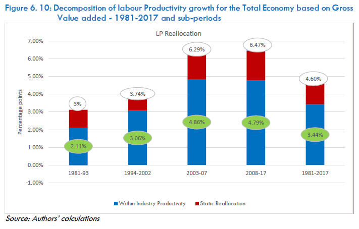 Note: The total may not sum up due to rounding off. The aggregate labour productivity growth rates for the total economy in Figure 6.10 differs marginally from the growth rates in Table 6.1 and 6.3, because while the growth rates in the figure are calculated from the change in the levels of labour productivity as given in equation 6.6, the labour productivity growth rates in Table 6.1 and Table 6.3 are the logarithmic growth rates. To further follow the evolution of reallocation effects, the annual trend is depicted in Figure 6.11. On considering static and dynamic effect separately, we observe that on an average, there has been almost no dynamic reallocation effect throughout the period and the index remains stagnant around the base value of 100. The dynamic effect has been contributing less, suggesting that employment has hardly been generated in sectors, which have witnessed faster labour productivity growth. The static reallocation effect, however, has been positive throughout the period, with steep rise since 2003-04, suggesting a positive structural change effect. In general, the effect of structural change — in terms of workers moving to sectors with high productivity level — on labour productivity growth has been positive, though the magnitude of the effect varies substantially over the years. Sectoral contribution to aggregate labour productivity growth In this section, we investigate the contribution of different sectors to aggregate labour productivity growth. While equation 6.5 gives aggregate labour productivity directly at the level of the aggregate economy, the second method to find the aggregate labour productivity growth is as the weighted sum of the 27 individual lpjt, with weights being the employment share of each industry ‘j’ (sjt) in total employment at time t. Hence, we may write  But while equation 6.5 gives the aggregate labour productivity, equation 6.7 provides within industry labour productivity and accounts for the changing weights of each industry over the period. In Figure 6.12, we summarise the broad sectors’ contribution to within industry labour productivity growth rate for the sub-periods and for the total period, and each broad sector’s contribution is expressed as a proportion of the aggregate productivity growth100. During 1981-1993, out of the within industry labour productivity growth rate of 2.11 per cent, it is the services sector that has dominated—contributing almost 46 per cent to productivity growth. While agriculture contributed 31 per cent, the manufacturing sector contributed 22 per cent, mining and electricity around 5-6 per cent each, but the construction sector experienced a decline in labour productivity. The picture has changed during the subsequent sub periods and in 2008-17 when within industry labour productivity growth has accelerated to 4.8 per cent, the contribution of services has also experienced a jump from 46 per cent to 54 per cent. The acceleration in labour productivity growth of the service sector might have induced some labour to shift from less-productive agriculture to services. Because of slow growth in labour productivity for both agriculture and manufacturing, their relative contribution has reduced between 1981-93 and 2008-17, from 31 per cent to 20 per cent for agriculture and from 22 per cent to 20 per cent for manufacturing. However, the contribution by the non-manufacturing industries (mining, electricity and construction) to labour productivity growth, which was almost negligible at 1 per cent during 1981-93, has gone up to 5.8 per cent in 2008-17. This has happened despite a massive shift of labour to the non-manufacturing sector whereby its employment share increased almost five-fold from a low of 2.8 per cent to 12.4 per cent from 1980 to 2017. It could partly be explained by its stagnant share in value added (at 2011-12 prices) at around 13.3 per cent. However, it does not mean that labour has shifted to a low-productivity sector, but it has basically shifted from one low-productivity sector, agriculture, to another low-productivity sector, ‘non-manufacturing’, but which has higher productivity than agriculture. It is supported by a positive static reallocation effect throughout the period as reflected in Figure 6.10. 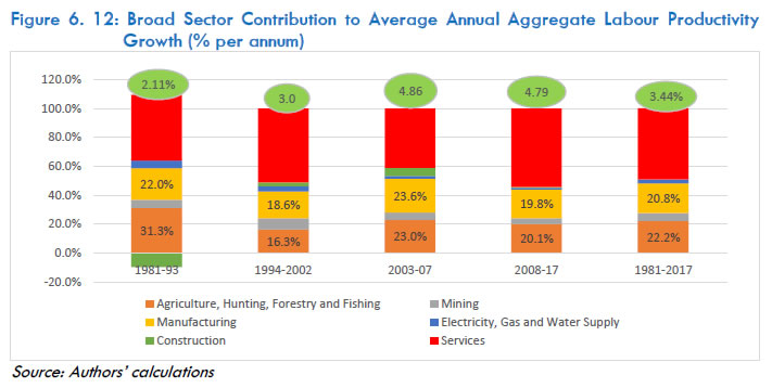 6.7 A cross-country comparison of labour productivity It is now worth exploring to see how India, having achieved a more than five-fold increase in the level of labour productivity for the aggregate economy during 1980-2017 (Figure 6.9) and an annual average growth rate of 4.5 per cent (Table 6.3, last row), compares with other developing countries. The comparison would help to view the trajectory of India’s labour productivity growth in the right perspective. This section compares India’s record on labour productivity growth at different points of time with the BRICS countries, other fast-growing economies in the region and advanced economies (Japan and the US). Table 6.4 indicates that India had the lowest labour productivity in 2017 except for Vietnam and Bangladesh—although it has one of the highest average annual growth rates among the selected countries both in GDP and labour productivity (second only after China) during 1981-2017. The Global productivity report (Dana, et.al., 2020, pp.265) confirms the result that the fast growth in productivity only narrowed down the productivity gap with the advanced-economy average but the level of productivity in South Asia, and especially India, remains the lowest among the EMDE countries. Despite an almost 6-fold increase between 1980 and 2017, India’s labour productivity in 2017 was only three-fourth of that of China, and Indonesia, and around one-half of Brazil and Thailand (Table 6.4). Further, it was a mere 20 per cent of that in Japan and 13 per cent of that in US. However, a comparison of India’s labour productivity and of other selected countries with that of China (China equal to one) reveals (Figure 6.13) that while China had almost the lowest level of labour productivity (almost equal to India) in 1980, India’s labour productivity in 2017 is only 75 per cent of China’s101. China, because of rapid growth in labour productivity during 1980 to 2017, has not only surpassed Bangladesh, Philippines, and Vietnam but has also narrowed down its gap with the other selected countries (Brazil, Indonesia, Russia, South Africa, and Thailand). If India wishes to emulate China and achieve the same economic might, then it also must narrow down the relative gap in labour productivity by adopting suitable policies to increase its labour productivity at a faster pace— not only to improve its economic growth but also the per capita income of its population. | Table 6.4: A cross country comparison of growth in GDP, growth in LP* and the level of LP* ($) | | Country | Average annual Growth in GDP
(1981-2017) (%) | Average annual Growth in LP
(1981-2017) (%) | Labour productivity in 1980 ($) | Labour productivity in 1994 ($) | Labour productivity in 2003 ($) | Labour productivity in 2008 ($) | Labour productivity in 2017 ($) | | Brazil | 2.2 | 0.3 | 28,674 | 25,581 | 26,520 | 29,342 | 31,169 | | Russian Federation | 0.9 | 0.9 | 41,724 | 31,293 | 39,726 | 52,280 | 55,277 | | India | 6.4 | 4.9 | 2,948 | 4,612 | 6,683 | 9,639 | 17,186 | | China | 7.0 | 5.6 | 3,098 | 5,178 | 8,509 | 13,275 | 23,016 | | South Africa | 2.2 | 0.2 | 43,520 | 34,027 | 40,612 | 44,776 | 46,525 | | Bangladesh | 5.2 | 3.0 | 3,852 | 4,681 | 5,866 | 7,471 | 11,542 | | Indonesia | 5.1 | 2.7 | 9,653 | 13,352 | 14,711 | 17,924 | 24,613 | | Malaysia | 5.8 | 2.8 | 22,286 | 37,458 | 43,774 | 53,492 | 60,291 | | Philippines | 3.7 | 1.2 | 14,046 | 11,213 | 12,791 | 15,019 | 21,003 | | Thailand | 5.3 | 3.9 | 8,588 | 18,974 | 22,310 | 25,428 | 33,400 | | Vietnam | 6.6 | 4.0 | 3,127 | 4,635 | 7,090 | 8,655 | 13,347 | | Japan | 2.5 | 2.2 | 36,439 | 56,398 | 70,004 | 74,217 | 79,731 | | United States | 3.0 | 1.8 | 67,123 | 85,832 | 108,312 | 117,021 | 130,811 | * Labour productivity per person employed in 2019 US$ (PPP)
Notes: The Chinese estimates are based on alternative GDP estimates by the Conference Board and will not be consistent with China’s official data. The official data would suggest Chinese labour productivity levels are slightly higher.
Source: Authors’ calculations from the Total Economy Database: Conference board, July 2020 version |
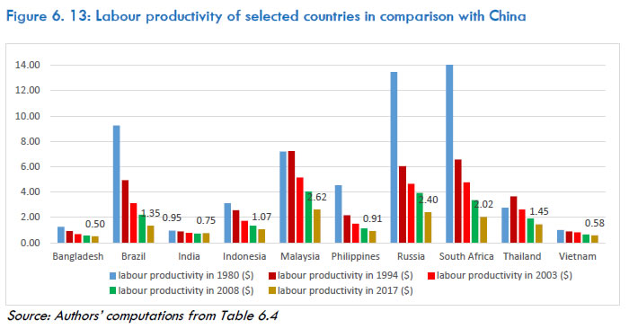 OECD (2016) has also analysed the paradox of falling growth in labour productivity despite substantive technological progress in many developed countries since mid-1990s. It provides a plausible explanation of the structural change in the economies in terms of a shift from the more-productive manufacturing towards growth of less-productive personal services (ibid, p.18). Based on an analysis of labour productivity across the globe, Dieppe (ed. 2020) has concluded that while labour productivity growth halved between 1980 and the beginning of the GFC, i.e., 2008 in the advanced countries, in the EMDEs it accelerated after the slowdown of the 1980s. However, after the 2008 GFC, the slowdown in productivity affected 70 per cent of all the economies, both advanced and EMDEs. The report (Dana, et.al., pp. 265) however, mentions that out of the six regions in EMDE, South Asia where India is the dominant economy, slowed only mildly after the GFC and its productivity growth was second fastest among these six regions at 5.3 per cent a year during 2013-18. India, however, seems to have buckled this trend with an acceleration in its labour productivity growth due to adoption of ICT by its dominant services sector. He finds that while slowdown of investment is the main reason for slowdown in productivity in advance economies during the last decade, the reason in the EMDEs is equal slowdown in both investment and TFP growth. The report (Dieppe, 2020, p. i17) finds that many different factors have affected long-term growth in labour productivity, but it mainly depends on ‘innovation, physical capital investment, and investment in human capital’. 6.8 Summary and Conclusion The chapter has estimated labour productivity for 27 industries across all sectors of the Indian economy for the period 1980-2017, wherein growth in labour productivity has been computed by the difference in the growth rate of value of gross value added and growth rate of persons employed by UPSS. The chapter has used the gross value-added approach in finding the sources of labour productivity growth. It finds that growth of labour productivity varies across industries. Chemical and chemical products grew the fastest with a growth rate of more than 6 per cent, followed by Other non-metallic mineral products, Public administration, Post & telecommunication, and Textile & leather products. On the other hand, Construction, Wood and wood products, Machinery, n.e.c., Other services, Transport & storage, and Pulp, Paper, etc. recorded very low (less than 3 per cent) growth in labour productivity, which raises an important concern regarding the possibility of improving the economic condition of the almost one-fourth of workforce that is employed collectively in these industries. This is pertinent as living conditions of workers generally depend on their labour productivity. The change in labour productivity between the two periods of 1994 to 2007 and 2008 to 2017 has also varied considerably — ranging from more-than 14 per cent to negative nine per cent. The analysis also reveals that labour productivity growth has been faster in industries that are more capital-intensive and the growth is also faster in ICT-producing and ICT-using industries than non-ICT industries. The drivers of labour productivity growth — capital deepening, labour quality or labour compositional changes, and TFP growth have also been estimated. In most (23 industries out of 27) industries, growth in capital intensity is the key driver, and TFP growth contributed significantly only to four industries. Evidently, it is factor accumulation that is leading to growth in labour productivity and the contributions of growth in labour composition and TFP growth are marginal—so more than the quality of factors, it is the quantity which is the main source of labour productivity growth. On the other hand, we find that TFP growth contributed a substantive 40 per cent to the aggregate labour productivity growth in the ICT-producing industries (three), 28 per cent in ICT-using industries (nine) even as it contributed a mere 4 per cent in the non-ICT industries (15). From a long-term perspective of growth of the economy, it is growth in TFP and growth in labour composition which are desirable and sustainable and not growth in capital deepening. Since out of total 27 industries, only 12 industries are either ICT-producing or ICT-using where TFP growth contribution is significant, the focus therefore must be on incentivising industries to either produce more or use more of ICT, in which India fortunately has a comparative advantage. It has also been found that a few industries in the Indian economy have followed the virtuous path of high growth in employment as well as high growth in labour productivity. These industries along with others with similar potential could be harnessed in the future through proper policy incentives to foster growth in employment and productivity. Industry decomposition of labour productivity growth shows that aggregate productivity growth is explained majorly by within industry productivity growth, and between industry or structural change explains only a marginal share. The static reallocation effect (within effect plus between effect) has been positive and is 25 percent of the aggregate productivity growth in the entire period 1980-2017, suggesting a positive structural change effect. The dynamic effect has been mostly negligible in most of the years, suggesting that employment has hardly been generated in sectors which were witnessing faster productivity growth. The analysis also makes it very clear that the major contribution to the aggregate productivity growth has come from the service sector in all the sub-periods, especially immediately after the reform process had begun in India in 1990s, and in 2008-17. A cross-country comparison, however, reveals that despite achieving one of the highest growths in labour productivity at an average of 5 per cent per annum during 1981-2017, the level of labour productivity in India is still very low in comparison with several other countries. With China as the benchmark, it is observed that while India and China had almost the same level of labour productivity in 1980, by 2018 the level in India had become just three-fourth of that in China. There is need for further investigation into the reasons for the low level of labour productivity in India. Some of the plausible reasons could be the increasing capital deepening where industry is substituting labour with capital because of the low cost of capital, mismatch of labour skills, rigid labour laws, obsolescence of technology in major sectors of agriculture and manufacturing, and emergence of the ‘new economy’ that is services-centred and require less, albeit skilled labour. Annexure 6A: Additional Table | Table 6A.1: List of KLEMS industries and capital intensity based and ICT based classification | | SL No | Industry code | KLEMS Industry Description | Capital intensity-based classification | ICT based classification | | 1 | AtB | Agriculture, Hunting, Forestry and Fishing | labour intensive | non-ICT | | 2 | C | Mining and Quarrying | High capital intensive | non-ICT | | 3 | 15t16 | Food Products, Beverages and Tobacco | Low capital intensive | non-ICT | | 4 | 17t19 | Textiles, Textile Products, Leather and Footwear | labour intensive | non-ICT | | 5 | 20 | Wood and Products of wood | labour intensive | non-ICT | | 6 | 21t22 | Pulp, Paper, Paper products, Printing and Publishing | Low capital intensive | ICT using | | 7 | 23 | Coke, Refined Petroleum Products and Nuclear fuel | High capital intensive | non-ICT | | 8 | 24 | Chemicals and Chemical Products | High capital intensive | non-ICT | | 9 | 25 | Rubber and Plastic Products | Low capital intensive | non-ICT | | 10 | 26 | Other Non-Metallic Mineral Products | Low capital intensive | non-ICT | | 11 | 27t28 | Basic Metals and Fabricated Metal Products | Low capital intensive | non-ICT | | 12 | 29 | Machinery, nec. | Low capital intensive | ICT using | | 13 | 30t33 | Electrical and Optical Equipment | Low capital intensive | ICT producing | | 14 | 34t35 | Transport Equipment | High capital intensive | ICT using | | 15 | 36t37 | Manufacturing, nec; recycling | labour intensive | ICT using | | 16 | E | Electricity, Gas and Water Supply | High capital intensive | ICT using | | 17 | F | Construction | labour intensive | non-ICT | | 18 | G | Trade | labour intensive | ICT using | | 19 | H | Hotels and Restaurants | labour intensive | non-ICT | | 20 | 60t63 | Transport and Storage | Low capital intensive | non-ICT | | 21 | 64 | Post and Telecommunication | High capital intensive | ICT producing | | 22 | J | Financial Services | Low capital intensive | ICT using | | 23 | 71t74 | Business Service | High capital intensive | ICT producing | | 24 | L | Public Administration and Defence; Compulsory Social Security | High capital intensive | non-ICT | | 25 | M | Education | labour intensive | ICT using | | 26 | N | Health and Social Work | labour intensive | ICT using | | 27 | 70+O+P | Other services | High capital intensive | non-ICT | | Source: Aggarwal (2018, pp.10) |
Chapter 7: Industry origins of Aggregate Growth and Total Factor Productivity 7.1 Introduction The purpose of this chapter is to examine in detail the industry origins of aggregate growth and productivity of the Indian economy. Economic growth has been subject to extensive research ever since the works of Solow (1957, 1970), Denison (1967) and Kuznets (1971). Kuznets indirectly maintained that US economic growth was largely attributable to the famous “Solow residual”, which was identified by Solow as a measure of technical change (1957). However, further investigation of the Solow residual (Griliches, 2000; Hulten, 2001) using more refined measures of factor inputs eventually attributed a lesser role for TFP than the traditional growth accounting approach followed by the early studies. Importantly, a seminal paper by Jorgenson and Griliches (1967) introduced constant quality indices for labour and capital inputs whilst also replacing the aggregate production function with the production possibility frontier102. These methodological enhancements resulted in capital and labour input accounting for the majority of the US economic growth studied in the paper, rather than TFP. They have also greatly influenced researchers’ understanding of the sources and origins of an economy’s growth, which has evidently become an important research agenda in the Indian context—given the country’s extensive preoccupation with GDP growth numbers. India’s economic growth has been a subject of regular debate in terms of its underlying sources and pitfalls. As highlighted in Bhandari and Kale (2015), it has been quite some time since India moved past the phase of ‘Hindu rate of growth’, with impressive growth performance attributable to initial ‘dipstick reforms’ in the 1980s (Ahluwalia, 1994), followed by the more systematic and comprehensive economic reforms in the 1990s. If reforms are connected to improved efficiency, then the link between the contribution of TFP growth towards output growth provides an immediate explanation for the growth-reform equation. Although what the Solow residual represents precisely is subject to academic debate, TFP growth has been convincingly argued to represent a useful indicator of welfare by Basu et al. (2014)103 and is widely considered as a yardstick of improvement in living standards. Given this context, growth and productivity measurement emerges as an important research area which has inevitably attracted the attention of Indian researchers. | Research based on the India KLEMS Database has provided a major turnaround in growth and productivity analysis. Moving beyond aggregate and sectoral perspectives it has focused on a disaggregated industry-level approach. | As highlighted in Chapter 1, many early studies have already analysed India’s productivity performance at the aggregate and sectoral level104. However, the creation of and dissemination of research based on the India KLEMS Database has provided a major turnaround in growth and productivity analysis. Research output of the India KLEMS Project has focused on moving beyond the aggregate and sectoral perspectives towards a more disaggregated industry-level approach—allowing researchers to analyse the considerable heterogeneity in the performance parameters of the 27 India KLEMS industries. This type of disaggregated analysis has been followed by several studies (Das et al., 2016, Goldar et al., 2017 and Erumban et al., 2019). This chapter carries forward such analysis by addressing the sources of India’s growth and productivity, using the approach outlined in Jorgenson et al. (2005). The major attribute of this chapter is its use of the Production Possibility Frontier (PPF) approach, which is methodologically superior over the more traditional method of using an Aggregate Production Function (APF). The application of the latter is particularly questionable when analysing the Indian economy (this is discussed in brief later in the chapter). The methodology adopted here enables quantification of the sources of growth at the industry-level in order to understand how changes in technology, production processes and input decisions across industries can contribute to aggregate economic growth. In addition, comparing the contributions of inputs—primary and intermediate—with the role of productivity improvement helps identify whether it is input accumulation or TFP growth that led to higher growth. The analysis also helps understand that if indeed there is an improvement in aggregate output and productivity growth, which industries are driving the origins of the observed growth patterns. These two aspects form the core of the present chapter. The analysis covers the overall period of 1980-17, supplemented by an important discussion regarding the change in output growth, input contributions and productivity performance following the Global Financial Crisis (GFC) of 2007-08. The latter discussion departs from the more widely covered growth and productivity dynamics pre- and post-economic reforms of the 1990s. The structure of the chapter is as follows. Section 7.2 provides an overview of research examining India’s productivity performance along with key findings. Section 7.3 provides the theoretical foundations underlying the methodology adopted in the chapter. Section 7.4 examines the industry origins/sources of growth and productivity by considering (1) sources of industry gross output growth, (ii) industry origins of aggregate value-added growth and productivity for the overall period of 1980-2017. Section 7.5 discusses the analysis of change in the above results from the pre-global financial crisis period to the post-crisis period i.e., 1993-07 and 2008-17. Section 7.6 provides a sectoral perspective by aggregating the results from the preceding sections. Section 7.7 concludes the chapter. Supplementary tables are presented in the Annexure. | Our use of the Production Possibility Frontier approach enables quantification of the sources of growth to see how industry-level changes in technology, production processes and input decisions can contribute to aggregate economic growth. | 7.2 Review of Indian Growth and Productivity Literature The Indian growth and productivity literature has evolved substantially in the 21st century, covering various sectors as well as the aggregate economy. We review the relevant literature in two categories—those that use non-KLEMS datasets with a variety of methodologies and those based on the India KLEMS dataset and growth accounting techniques. 7.2.1 Studies based on non-India KLEMS datasets A good starting point here would be to address the enormous literature that attempts to establish the link between economic reforms and growth of the Indian economy. Virmani (2005) discusses the break points of various growth phases during 1950-2002. The results indicate that the growth turnaround occurred during the 1980s—the period of piecemeal reforms. In an earlier study, De Long (2004) noted that the policies of central planning and “licence-raj” coupled with an attraction to Fabian Socialism under the Nehruvian era created a growth-deceleration effect, which was overturned by growth acceleration in the late 1980s. Panagariya (2004) identified the high growth period of 1988-91 as one which boosted the average growth rate of the 1980s. Rodrik and Subramanian (2005) pointed out that the growth transition in the 1980s is attributable to the attitudinal shift of the government in favour of the private sector, which evoked a large productivity response facilitated “by the fact that India was far away from its income-possibility frontier.” However, as discussed in Joshi and Little (1994), the growth expansion of the 1980s came with large fiscal deficits, financed by some internal but largely by external borrowings—an unsustainable formula which eventually led to the balance of payment crisis in 1991. Overall, the literature suggests that while the piecemeal reforms of the 1980s had an important influence on India’s growth trajectory, the subsequent growth expansion was not a healthy one. In contrast, the robust systematic reforms of the 1990s were necessary to keep the output and productivity growth alive. If reforms raise efficiency, the link between reforms and economic growth can be understood by evaluating the contribution of TFP growth to output growth. Several non-KLEMS dataset studies have worked on deciphering this link at the aggregate and sectoral levels. Bosworth et al. (2007) base their growth accounts on an Aggregate Production Function (APF) approach with a value-added Cobb-Douglas production function specification to analyse growth and productivity of the aggregate economy and three sectors—agriculture, industry, and services. Notably, the study finds that the post-1980 (1980-04) aggregate acceleration in output growth of 5.8 per cent per annum is majorly attributable to the TFP growth of 2 per cent per annum—indicating the reform-growth link during this period. The study finds that the largest post-1980 (1980-04) annual output growth was witnessed in the services sector at 7.6 per cent, mainly driven by the sector’s annual TFP growth of 2.9 per cent during this period. Goldar and Mitra (2008) analysed growth and productivity of the services sector in greater detail. They found that the post-1980 turnaround in TFP growth of this sector was determined in large part by increase in TFP growth of trade, hotels and restaurants, and public administration and other community services. Eichengreen and Gupta (2011) found that services such as communications, business services, financial services, education, healthcare, and hotels explained most of the post-1990 acceleration in services growth. Based on firm-level panel data for 1993-05 and services-reform indices, Arnold et al. (2016) found the rise in service sector productivity significantly linked to manufacturing productivity. Against firm-level TFP growth, they found significant positive coefficients for individual services-reform indices for banking, insurance, telecom, and transport services. | The literature suggests that while the piecemeal reforms of the 1980s had an important influence on India’s growth trajectory, the subsequent expansion was not a healthy one. The robust systematic reforms of the 1990s were necessary to keep the output and productivity growth alive. | Analysis of Indian manufacturing growth and productivity has also received great attention by the existing literature. Trivedi et al. (2011) provides a comprehensive overview of datasets, methodologies and estimates of the studies pertaining to this sector and presents the stylised facts established in the existing literature. They found that for 1980-81 to 2003-04, estimates of TFP growth for the organised manufacturing are sensitive to the methodology applied. For this period, a growth accounting approach (non-parametric) based on a discrete translog production function results in a trend TFP growth rate of 0.92 per cent per annum. However, the estimation of TFP growth from a Cobb-Douglas production function approach (parametric) gives a corresponding trend figure of 1.81 per cent per annum. This translates into contribution of TFPG to output growth of organised manufacturing by these two approaches between 13 to 25 per cent, respectively. Notably, in the context of the systematic reforms of the 1990s, the study found a statistically significant decline in TFP growth in the post-reform period of 1992-93 to 2003-04 against the pre-reform period of 1980-81 to 1991-92. For registered and unregistered manufacturing, Bosworth et al. (2007) found that TFP growth slowed in 1993-99 period compared with the previous sub-period of 1983-93, and rebounded during 1999-2004. In contrast, studies such as Krishna and Mitra (1998) and Pattnayak and Thangavelu (2005) found an increase in manufacturing TFP growth during the 1990s. In terms of growth and productivity of agriculture, Kumar and Mittal (2006) provide a comprehensive review of empirical studies that have investigated TFP growth for this sector. Sakia (2009) found that TFP growth declined in the 1990s after increasing during the 1980s. Several studies (Rosegrant and Evenson, 1992; Evenson et al., 1999; Fan et al., 1999, Dholakia and Dholakia, 1999) find an acceleration in the TFP index for Indian agriculture after the introduction of high yielding varieties. Overall, the literature suggests that the agricultural productivity attained during the 1980s was not sustained in the 1990s (Kumar and Mittal, 2006). 7.2.2 Studies based on the India KLEMS datasets Studies based on the India-KLEMS dataset have been able to push the growth and productivity literature beyond the sectoral and aggregate perspective, by building industry-production accounts at the disaggregated level of 27 industries. An important recent study by Goldar et al. (2017), closely resembling the PPF methodology of this chapter, used the India-KLEMS dataset version of 2016 to analyse growth, structural change, and productivity of the Indian economy during 1980-2014. The trend annual growth rate of aggregate value-added was found to have progressed from 5 per cent in 1980-93, to 5.8 per cent in 1994-02 and 7.5 per cent during 2003-14. Notably, the study showed that the real value-added share of the manufacturing sector does not stagnate when a double deflation approach is applied, in contrast to the stagnant manufacturing share observed when using a single deflated value-added series. In terms of aggregate TFP growth, the study carried out a Domar aggregation exercise which revealed that manufacturing, non-market services and market services were the largest contributors to the aggregate TFP growth for 1980-14. The dynamics of structural changes were analysed by decomposing labour and capital productivity with the assumption of an Aggregate Production Function (APF). For both labour and capital productivity during 1980-14, the study found that although within-industry productivity growth accounted for most of the labour and capital productivity growth, positive static reallocation effects were present and were relatively substantial compared with dynamic reallocation effects. Das et al. (2016) is a major attempt to highlight India’s productivity performance under different policy regimes. The study identifies that liberal market reforms in the 1990s seem to have benefitted market services in expanding investment, productivity, and growth in the post reform period, while helping manufacturing productivity through a long period of intensive capital accumulation. Erumban et al. (2019) followed the Goldar et al. study by utilising the assumption of an APF to decompose labour productivity growth and found results similar to the latter study. Additionally, using the Direct Aggregation across Industries (DAI) extension of the PPF approach, the study found that labour and capital reallocation effects (in accounting for aggregate TFP growth) were around 17 per cent per annum and 10 per cent per annum, respectively, for 1981-2011. Notably, the capital reallocation effect was negative for 1981-92, indicating that investment was flowing to industries with lower returns to capital during this period. However, the capital reallocation effect was positive and substantially higher than the labour reallocation effect since the mid-1990s till 2011—indicating that during this period, investment expanded in industries where capital was more productive. Das and Nath (2017) highlight “capital misallocation and its implications for India’s potential output”. They show that several sub-sectors in the services sector appear to be ‘over-capitalised’. On the other hand, several manufacturing subsectors are ‘under-capitalised’. Their results imply that aggregate output would have been higher by 20-30 per cent between 1990 and 2004 and 40 per cent between 2005 and 2012 had the distortions in capital allocation been removed. They conclude that a policy framework enabling ease of capital movement across sectors may be adopted for achieving higher growth. Aggarwal and Goldar (2019) performs an important investigation into the structure and trends of employment growth in the Indian economy for the period 1980-81 to 2015-16. The authors utilise the employment time series from the India KLEMS dataset to find point elasticity of employment instead of arc elasticity. Exemplifying the well-known pattern of jobless growth in the Indian economy, the authors find that impressive GDP growth after 1991 did not see commensurate growth in employment, especially during 2003-15 when employment elasticity stood at 0.1—a percentage point increase in GDP growth during this period led to 0.1 per cent increase in employment. Krishna et al. (2020) used an econometric approach using GMM (Generalised Methods of Moments) regression for a panel data model of TFP index as a function of measures for participation in GVCs (Global Value Chains), for the 12 India KLEMS manufacturing industries. The analysis for 1993-2015 revealed that the foreign value added (FVA) content in production had a significant positive coefficient, indicating that participation in GVCs helped the Indian manufacturing sector achieve higher productivity levels. Further, higher equipment share in total capital stocks was also found to be productivity enhancing. Productivity trends in the manufacturing sector has been explored in detail by Krishna et al. (2018), with a focus on formal and informal segments, for 1980-81 to 2011-12. The informal segments were expectedly found to be less efficient, indicating a need to raise output and employment of the formal segment. 7.3 Methodology 7.3.1 Production Possibility Frontier (PPF) approach The initial empirical results in this chapter are based on the usual growth accounting decomposition of gross output growth as outlined previously in Equation (2.5) of Chapter 2, under the assumptions of constant returns to scale and perfectly competitive input markets. We show the same equation here for exposition purposes: Let the production function be defined as: where X is intermediate input, L is labour input, K is capital input and A indicates technology. The concept of value added requires the existence of a value-added function which is separable in primary inputs (L and K) and technology A. This means that the production function can be written in the following form: where the function V(.) denotes the value-added function. With the separability condition shown in the above equation, the following equation holds for real gross output, real value of intermediate input and real value-added growth for any industry j: Once industry value-added growth is found from equation (7.4), the aggregate value-added growth (Δ ln V) from the production possibility frontier is given by the Törnqvist index of the industry value added growth as: Using the aggregate value-added growth in (7.6) and unweighted aggregate level measures of capital input and labour input, aggregate TFP growth rate from can be arrived at by: It should be noted that the above equation also holds when the concept of an APF is used i.e., underlying this relationship, one can define an aggregate production function as: 7.3.2 Direct Aggregation across Industries Once we have the estimates from the PPF, we use the least restrictive “Direct Aggregation across Industries”111 approach to estimate industry-level sources of aggregate growth and productivity. With reference to Jorgenson et al. (2007), this approach maintains the assumption of the existence of a value-added function for each industry. However, it imposes no cross-industry restrictions on either value-added or prices of inputs, which conveniently eliminates the assumptions of identical value-added functions, mobility of inputs across industries and equal factor prices for all industries. Substituting equation (7.5) into equation (7.6), gives the following expression for aggregate value-added growth: The impact of the assumptions behind the PPF can be quantified by decomposing aggregate TFP growth from equation (7.8); by subtracting equation (7.8) from (7.10), algebraic manipulations yield the following equation: 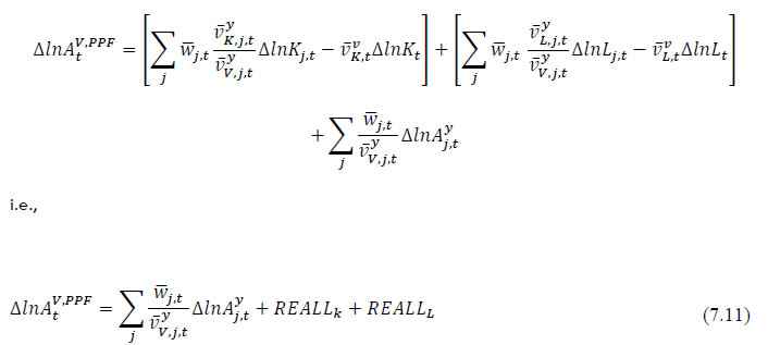 The first source of aggregate TFP growth is the sum of Domar-weighted industry TFP growth rates, while the second and third terms reflect the reallocation of capital and labour, respectively. If the latter terms are positive, a divergence is created between aggregate TFP growth rate and the sum of Domar-weighted industry TFP growth rates. In the above decomposition, theoretically, the reallocation terms can be used to quantify the departure from the assumptions on inputs required by both the APF and PPF approach (since equation (7.8) holds for either approach). If the reallocation terms are positive, aggregate TFP growth rate from the PPF will exceed the sum of Domar-weighted industry TFP growth rates. This, in turn, will happen when capital and labour inputs command different prices in different industries and the industries with higher prices have faster input growth rates, while aggregate capital or labour inputs grow more slowly than weighted averages of their industry counterparts. 7.3.3 Sectoral Aggregation For the purpose of analysing sectoral performance, we group the 27 India KLEMS industries into six main sectors, namely—Agriculture, Mining, Manufacturing, Utilities, Construction and Services. Further, three sub-sectors are also explicitly classified within the Manufacturing sector, these include— “Manufacturing of Consumer Goods”, “Manufacturing of Intermediate Goods” and “Manufacturing of Investment Goods”. The Services sector is also broken down into two sub-sectors—“Non-Market Services” and “Market Services”. The list of industries classified under these groups can be found in Table 7A.1 of Annexure 7A at the end of this chapter. The framework outlined above provides a useful way to quantify the sectoral contributions to aggregate value-added growth and TFP, directly from the industry-level estimates. To estimate the sectoral contributions to aggregate value-added growth, one can simply rewrite equation (7.6) in the following manner: In the above equation, the first two terms are the summation of industry-level contributions to aggregate value-added growth for the industries belonging to the Manufacturing and Services sector, respectively. Since there is only one industry falling under each of the latter three groups i.e., Agriculture, Mining and Utilities (refer to Table 7A.1 of Annexure 7A), the contributions of these sectors are equal to the industry contributions of each industry that falls within that sector. Similarly, one can arrive at sectoral contributions to aggregate TFP growth by breaking down the summation of Domar-weighted TFP contributions as: 7.4 Disaggregated Empirical Results, 1980-17 This section presents the estimates of growth and productivity at the disaggregated level of 27 India KLEMS industries, for the overall study period of 1980-17. The results of this section follow the growth accounting methodology as described in Section 2.2 of Chapter 2. The analysis of the disaggregated industry-level sources and origins of growth and productivity is the appropriate starting point since the performance of the aggregate economy is built from the industry-level production accounts. 7.4.1 Sources of Industry-level Output Growth The gross output of an industry is defined as the value of production created using primary factors such as labour and capital, and intermediate inputs purchased from other industries. As per the growth accounting methodology outlined in Jorgenson et al. (2005) and discussed in Chapter 2, the gross output of each industry is defined as a function of capital, labour, intermediate inputs, and technology. An important advantage of using the gross output framework is that it provides a complete measure of production and treats all inputs—labour, capital, and intermediate inputs—symmetrically. In contrast, the value-added measure of output does not explicitly account for the flow of intermediate inputs that may be the primary component of an industry’s output.113 Thus, we begin with the gross output production function to arrive at an accurate representation of India’s industries.114 By utilising industry-level gross output growth decomposition as shown previously in equation (7.1), we arrive at industry-level estimates as summarised in Table 7.1. The industry average and industry median are provided for each variable, which helps us identify whether the frequency distribution of the respective variable has a positive or a negative skew. The first column of Table 7.1 provides annual average estimates of gross output growth at the industry level for the overall period of 1980-2017115. It is observed that the 27 industries saw an average annual output growth rate of around 7.39 per cent, while the industry median was slightly lower at 7.33 per cent. Based on the Shapiro-Wilk test, we find evidence that the output growth rates follow a normal distribution.116 This indicates that the majority of the output growth rates were closer to the industry mean of 7.39 per cent per annum. Only a few industries experienced high output growth rates when annually averaged over the 1981-2017 period—Business services (12.4 per cent), Electrical & optical equipment (11 per cent), Other manufacturing (11 per cent), Rubber & plastic products. (10.2 per cent) and Post & telecom (9.9 per cent). The Agriculture & allied industry saw the lowest output growth rate at 2.81 per cent per annum for 1981-2017. | The gross output framework treats all inputs—labour, capital, and intermediate inputs—symmetrically, while the value-added measure of output does not explicitly account for the flow of intermediate inputs that may be the primary component of an industry’s output | The second column of Table 7.1 provides annual average estimates of capital input contribution to the observed output growth during 1980-2017. When compared with other inputs and TFP, for the majority of the 27 industries, capital input contribution emerges as the second most important source of output growth after intermediate inputs. Moreover, it is also the dominant source of output growth for a few, namely—Trade, Mining & quarrying, Financial Services, Education, Other Services and Wood and wood products. Overall, the industry average for capital input contribution stood at around 2 per cent, higher than the industry median of 1.60 per cent—implying a positive skew of the frequency distribution, as observed previously for industry output growth rates. A few industries saw relatively larger capital input contribution compared with the mean and these include—Business services, Trade, Mining and quarrying, Financial Services, and Non-metallic mineral products. It is a cause for concern that the contribution of labour input is relatively low (Table 7.1, column 3). The industry average for labour input contribution stood at 0.78 per cent, which is less than half (two-fifths) of the average contribution of capital input. A few exceptions to the generally low labour input contributions include a few service sector industries—Education, Business Services, Financial services, Other Services and Health & social work—and the Construction industry. Education industry is the only instance when labour input is the dominant contributor relative to other inputs. | Table 7.1: Gross Output Growth Decomposition, 1981-17 | | KLEMS Industry Description | Output Growth | Capital Input contribution | Labour Input Contribution | Intermediate Input contribution | TFP contribution | | Agriculture & allied | 2.81 | 1.32 | 0.10 | 0.54 | 0.85 | | Mining & quarrying | 5.50 | 3.47 | 0.46 | 3.01 | -1.45 | | Food pdts., beverages & tobacco | 7.59 | 0.91 | 0.22 | 5.76 | 0.70 | | Textiles & leather | 7.33 | 1.48 | 0.21 | 5.00 | 0.64 | | Wood & wood pdts. | 1.16 | 1.85 | 0.03 | 1.41 | -2.13 | | Pulp & paper pdts. | 6.42 | 1.00 | 0.54 | 4.66 | 0.22 | | Coke & petroleum pdts | 6.09 | 1.47 | 0.03 | 5.25 | -0.67 | | Chemicals & chemical pdts. | 7.65 | 1.30 | 0.31 | 5.78 | 0.25 | | Rubber & plastic pdts. | 10.27 | 2.68 | 0.30 | 6.39 | 0.90 | | Non-metallic mineral pdts. | 8.21 | 2.91 | 0.25 | 5.08 | -0.02 | | Basic metals & metal pdts. | 7.21 | 1.60 | 0.25 | 5.03 | 0.33 | | Machinery, nec. | 7.71 | 2.27 | 0.55 | 4.21 | 0.67 | | Electrical & optical eqpt. | 11.07 | 1.28 | 0.68 | 6.64 | 2.47 | | Transport eqpt. | 9.00 | 1.74 | 0.35 | 6.31 | 0.60 | | Other manufacturing | 11.05 | 1.44 | 0.69 | 7.13 | 1.79 | | Utilities | 7.33 | 1.58 | 0.39 | 4.29 | 1.06 | | Construction | 6.03 | 0.80 | 1.81 | 4.79 | -1.37 | | Trade | 6.97 | 4.07 | 1.33 | 1.48 | 0.09 | | Hotels & restaurants | 6.08 | 1.03 | 0.61 | 4.43 | 0.00 | | Transport & Storage | 7.08 | 0.89 | 1.10 | 4.43 | 0.66 | | Post & telecom | 9.97 | 2.47 | 0.70 | 6.34 | 0.45 | | Financial services | 8.72 | 3.36 | 1.63 | 2.29 | 1.44 | | Business services | 12.40 | 5.15 | 2.34 | 5.38 | -0.47 | | Public administration | 5.94 | 0.87 | 0.33 | 1.67 | 3.07 | | Education | 7.86 | 2.48 | 2.56 | 1.33 | 1.49 | | Health & social work | 6.62 | 2.16 | 1.50 | 2.39 | 0.57 | | Other services | 5.56 | 2.07 | 1.63 | 1.25 | 0.61 | | Industry Median | 7.33 | 1.60 | 0.54 | 4.66 | 0.60 | | Industry Average | 7.39 | 1.99 | 0.78 | 4.16 | 0.47 | | Source: Authors’ computations based on the India KLEMS Dataset version 2019 | The respective contribution of primary inputs to output growth can also be broken down into quality and quantity components (refer to Chapter 2 for more details). Figure 7.1 provides this breakdown for the overall period of 1981-2017. From Panel A, it is evident that capital stock contribution makes up for majority of the capital input contributions across the 27 industries, whereas capital quality contributions remained negligible. Looking at Panel B however, it is observed that labour quality is the dominant source over employment contributions for four industries—Public administration, Wood & wood products, Mining & quarrying, and Agriculture & allied. 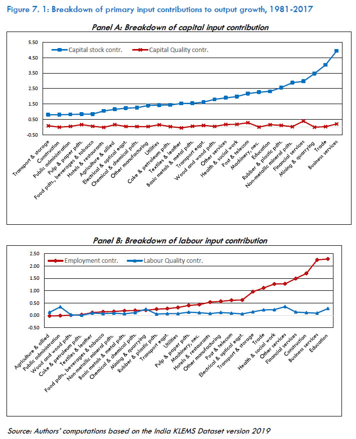 In column 4 of Table 7.1, we provide the contributions of intermediate inputs to output growth, which is the aggregate of Energy (E), Material (M) and Services (S) inputs. The industry average contribution of intermediate inputs was 4.16 per cent, while the industry median was higher at 4.66 per cent. Thus, contrary to the case of primary inputs, we identify a negative skewness in the frequency distribution of intermediate input contribution—indicating that majority of industries saw higher than average contributions from intermediate inputs. Intermediate inputs are subsequently observed to be the dominant source of output growth for 20 out of the 27 KLEMS industries. The rest seven industries (four of which belong to the Services sector) include Agriculture & allied, Mining & quarrying, Wood & wood products, Trade, Financial services, Education and Other Services. Except for the Education industry (which saw dominant contribution from labour input as noted previously), each of the remaining six industries saw capital input as the major contributor towards their respective output growth. Overall, it is found that for the industries belonging to the Manufacturing sector, intermediate inputs are by far the most important contributor to the observed growth except for the Wood & wood products industry. Given the observed importance of intermediate inputs, we provide separate estimates of Energy, Materials and Services contribution to the output growth of the 27 industries for the overall period of 1980-2017 (see also the discussion on this aspect in Chapter 3). From Table 7.2, we observe that Materials input drives most of the intermediate input contribution for the majority of the industries, especially those belonging to the Manufacturing sector. The average contribution of Material input across the 27 industries is around 2.63 per cent, which is substantially higher than the corresponding average figure for Energy (0.35 per cent) and Services input contribution (1.18 per cent). However, the contribution of the Services input is the dominant source of intermediate input contribution for nine industries, namely—Agriculture & allied, Utilities, Trade, Transport & storage, Financial services, Business services, Public administration, Education, and Other Services. Except for the Agriculture & allied and Utilities industry, the latter six industries belong to the Services sector itself. This result reflects the importance of inter-industry linkages within the Services sector. Finally, it is observed that Energy input contribution remains negligible for most of the industries, the only exception being the Utilities and the Transport & storage industry. | Table 7.2: Energy, Material & Services input contribution to output growth, 1981-2017 | | KLEMS Industry Description | Intermediate Input Contribution | Energy Input Contribution | Material Input Contribution | Services Input Contribution | | Agriculture & allied | 0.54 | 0.07 | 0.21 | 0.26 | | Mining & quarrying | 3.01 | 0.35 | 1.68 | 0.99 | | Food pdts., beverages & tobacco | 5.76 | 0.11 | 4.14 | 1.51 | | Textiles & leather | 5.00 | 0.22 | 3.66 | 1.11 | | Wood & wood pdts. | 1.41 | -0.01 | 1.17 | 0.24 | | Pulp & paper pdts. | 4.66 | 0.35 | 3.37 | 0.94 | | Coke & petroleum pdts | 5.25 | 0.13 | 5.07 | 0.05 | | Chemicals & chemical pdts. | 5.78 | 0.21 | 4.76 | 0.81 | | Rubber & plastic pdts. | 6.39 | 0.24 | 4.99 | 1.16 | | Non-metallic mineral pdts. | 5.08 | 1.16 | 2.81 | 1.11 | | Basic metals & metal pdts. | 5.03 | 0.77 | 3.16 | 1.10 | | Machinery, nec. | 4.21 | 0.08 | 3.33 | 0.80 | | Electrical & optical eqpt. | 6.64 | 0.24 | 4.79 | 1.61 | | Transport eqpt. | 6.31 | 0.48 | 4.35 | 1.48 | | Other manufacturing | 7.13 | 0.16 | 5.24 | 1.73 | | Utilities | 4.29 | 1.25 | 1.33 | 1.71 | | Construction | 4.79 | 0.17 | 3.03 | 1.59 | | Trade | 1.48 | 0.21 | 0.31 | 0.96 | | Hotels & restaurants | 4.43 | 0.18 | 3.20 | 1.05 | | Transport & Storage | 4.43 | 1.49 | 1.14 | 1.80 | | Post & telecom | 6.34 | 0.76 | 4.09 | 1.49 | | Financial services | 2.29 | 0.22 | 0.44 | 1.64 | | Business services | 5.38 | 0.40 | 1.63 | 3.35 | | Public administration | 1.67 | 0.02 | 0.31 | 1.33 | | Education | 1.33 | 0.03 | 0.24 | 1.05 | | Health & social work | 2.39 | 0.03 | 2.07 | 0.29 | | Other services | 1.25 | 0.02 | 0.59 | 0.63 | | Industry Average | 4.16 | 0.35 | 2.63 | 1.18 | | Source: Authors’ computations based on the India KLEMS Dataset version 2019 | The final source of industry output growth is Total Factor Productivity (TFP) contribution, estimates of which are provided in the last column of Table 7.1.117 The industry median value of 0.60 per cent TFP per annum is slightly greater than the industry average of 0.47 per cent per annum. Given, the close mean and median values, our analysis based on the Shapiro-Wilk test confirmed the existence of normality in industry TFP growth rates.118 Relative to the other three inputs, we observe that TFP contribution to output growth was substantially lower for the period 1981-2017. The negative or negligible contribution from TFP is reflected across all the industries except for only a few industries—Public administration, Electrical & optical equipment, Other manufacturing, Education and Financial Services. Notably, the Public administration industry presents the only case where TFP contribution to output growth is greater than the corresponding contributions from the other inputs. As highlighted in Das et al. (2019), TFP growth in Public administration is difficult to explain since this industry does not follow market principles and wages are administered by government decisions. Therefore, the ratio of output to input may not necessarily reflect productivity in this sector.119 7.4.2 Industry Origins of Aggregate Growth and Productivity Having explored the industry-level sources of output growth, it is important to ascertain which industries are driving aggregate-level growth and productivity. As mentioned previously, we use the Production Possibility Frontier (PPF) approach supplemented by the methodology of Direct Aggregation across Industries (DAI) (as outlined in section 7.4), to carry out the required analysis. Ignoring the summation sign, we refer to the term on right-hand side of equation (7.6) as industry contributions to aggregate value-added growth (CTVA,j,t) and the third term on the right of equation (7.10) as the industry contributions to aggregate TFP growth (CTTFP,j,t). These two terms can be rewritten as:  Table 7.3 provides estimates from the above equation by separating the respective weights and growth rates used to estimate CTVA,j,t and CTTFP,j,t. Since this section provides estimates that are annually averaged over the period of 1981-2017, there is a substantial potential of masking the underlying variations. Figure 7.2 ranks the industries according to the estimates of CTVA,j for the overall period of 1981-17. The industries making the first five largest contributions are—Agriculture & allied, Trade, Other services, Business services, and Financial services. Although these five industries account for more than half of the aggregate value-added for the period considered, the Agriculture & allied industry itself accounts for a quarter of the aggregate value added. As can be seen from Table 7.3, the value-added growth of the Agriculture & allied industry was only 3.11 per cent, the second lowest among the 27 industries, indicating that this industry's large contribution was emancipated from its large size in the economy rather than high growth. In contrast, the contributions of the other four industries, all four from the service sector, are driven by relatively strong value-added growth rates and value-added shares. Interestingly, even when we consider the top 10 contributors, they are predominantly service sector industries, except Construction and Utilities, which make relatively large contributions of around 0.28 per cent and 0.24 per cent, respectively. As for the industries belonging to the Manufacturing sector, none are within the list of top 10 contributors. The relatively smaller contributions from the Manufacturing industries result from their minor share in aggregate value-added rather than slow value-added growth. Several Manufacturing industries experienced high rates of value-added growth rates, including Electrical & optical eqpt., Rubber & plastic products, Other manufacturing, and Transport equipment. 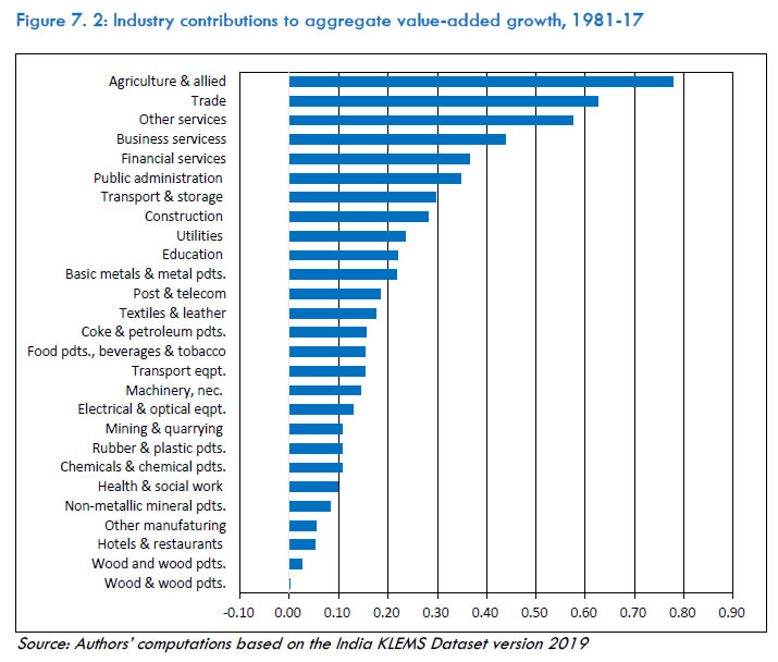
| Table 7.3: Industry contributions to aggregate value-added and TFP growth, 1981-2017 | | Sl. No. | KLEMS Industry Description | Value-Added (VA) | Total Factor Productivity (TFP) | | VA Share | VA Growth | Contribution to Aggregate VA Growth | Domar Weight | TFP Growth | Contribution to Aggregate TFP Growth | | 1 | Agriculture & allied | 0.249 | 3.11 | 0.78 | 0.35 | 0.85 | 0.28 | | 2 | Mining & quarrying | 0.029 | 4.03 | 0.11 | 0.05 | -1.45 | -0.08 | | 3 | Food pdts., beverages & tobacco | 0.019 | 8.24 | 0.15 | 0.09 | 0.70 | 0.06 | | 4 | Textiles & leather | 0.025 | 7.40 | 0.18 | 0.08 | 0.64 | 0.05 | | 5 | Wood & wood pdts. | 0.006 | -0.26 | 0.00 | 0.01 | -2.13 | -0.03 | | 6 | Pulp & paper pdts. | 0.005 | 4.88 | 0.03 | 0.02 | 0.22 | 0.00 | | 7 | Coke & petroleum pdts | 0.012 | 6.91 | 0.16 | 0.11 | -0.67 | 0.01 | | 8 | Chemicals & chemical pdts. | 0.019 | 6.53 | 0.11 | 0.06 | 0.25 | 0.00 | | 9 | Rubber & plastic pdts. | 0.008 | 12.82 | 0.11 | 0.03 | 0.90 | 0.03 | | 10 | Non-metallic mineral pdts. | 0.011 | 7.72 | 0.08 | 0.03 | -0.02 | -0.00 | | 11 | Basic metals & metal pdts. | 0.028 | 7.81 | 0.22 | 0.10 | 0.33 | 0.03 | | 12 | Machinery, nec. | 0.015 | 9.74 | 0.15 | 0.04 | 0.67 | 0.03 | | 13 | Electrical & optical eqpt. | 0.009 | 14.21 | 0.13 | 0.03 | 2.47 | 0.07 | | 14 | Transport eqpt. | 0.015 | 10.42 | 0.15 | 0.06 | 0.60 | 0.04 | | 15 | Other manufacturing | 0.005 | 10.46 | 0.05 | 0.02 | 1.79 | 0.03 | | 16 | Utilities | 0.027 | 8.65 | 0.24 | 0.08 | 1.06 | 0.09 | | 17 | Construction | 0.071 | 3.45 | 0.28 | 0.20 | -1.37 | -0.25 | | 18 | Trade | 0.086 | 7.18 | 0.63 | 0.11 | 0.09 | -0.00 | | 19 | Hotels & restaurants | 0.009 | 5.93 | 0.05 | 0.03 | -0.00 | -0.00 | | 20 | Transport & Storage | 0.047 | 5.99 | 0.30 | 0.10 | 0.66 | 0.09 | | 21 | Post & telecom | 0.016 | 9.41 | 0.18 | 0.04 | 0.45 | 0.05 | | 22 | Financial services | 0.046 | 8.41 | 0.36 | 0.06 | 1.44 | 0.08 | | 23 | Business services | 0.038 | 10.86 | 0.44 | 0.06 | -0.47 | -0.03 | | 24 | Public administration | 0.059 | 5.87 | 0.35 | 0.08 | 3.07 | 0.25 | | 25 | Education | 0.028 | 7.76 | 0.22 | 0.03 | 1.49 | 0.05 | | 26 | Health & social work | 0.012 | 7.63 | 0.10 | 0.02 | 0.57 | 0.01 | | 27 | Other services | 0.107 | 5.13 | 0.58 | 0.13 | 0.61 | 0.11 | | | TOTAL | 1.00 | | 6.12 | 2.00 | | 0.96 | | Source: Authors’ computations based on the India KLEMS Dataset version 2019 | Before discussing the industry-level contributions to aggregate TFP growth, it is important to note that according to theory, the Domar weights typically add up to more than one (they add up to exactly two in our case, as shown in the last row of Table 7.3). This usually implies that in the presence of intermediate transactions between the industries (or the use of intermediate inputs), aggregate productivity growth will be greater than the weighted average growth rates of the industries. This means, productivity gains from the production of intermediate inputs have an additional effect of reducing input prices in downstream industries.120 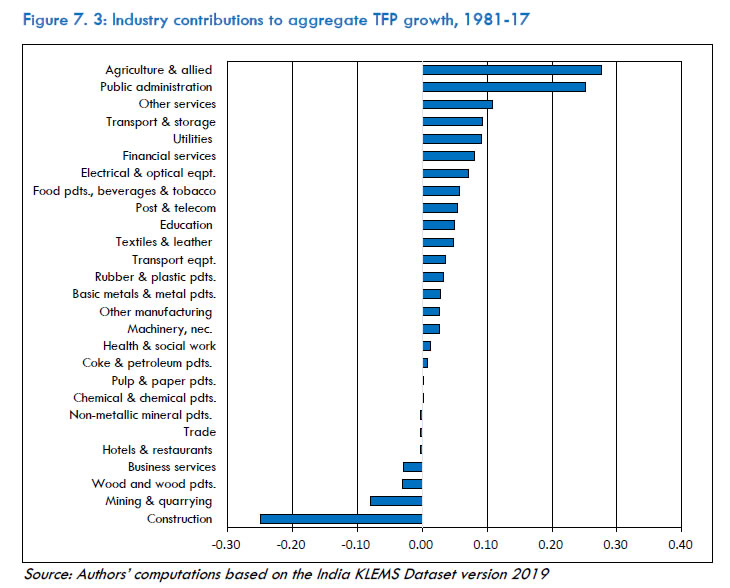 Figure 7.3 provides the ranking of industries in terms of their (Domar-weighted) contributions to aggregate TFP growth (CTTFP,j) for the overall period of 1981-2017. As in the case of value-added growth, Agriculture & allied industry retains its position as the largest contributor to aggregate TFP growth. The other substantial contributors include – Public administration121, Other services, Transport & storage, and Utilities. Unlike the contributions to aggregate value-added growth, the industry contributions to aggregate TFP growth are negative for a small subset of industries, namely—Construction, Mining & quarrying, Wood & wood products and Business services. Thus, we observe substantial heterogeneity in terms of industry contributions to aggregate TFP growth. The construction sector seems to be the largest drag on aggregate TFP growth. It is a relatively less skill-intensive sector than manufacturing and operates largely in the informal sector. Given these two features, previous studies have observed that much of the fall in jobs in agriculture has been compensated in a rise in employment in the construction sector, but with no added productivity gains (Erumban et al., 2019). 7.4.3 Industry contributions to growth of aggregate primary inputs As highlighted in equation (7.10), the PPF approach allows useful extension to the DAI method, which in turn, allows us to trace the origins of aggregate primary input accumulation to its industry sources. For exposition, we rewrite the necessary components previously defined in equation (7.10) as: where the first and second term refer to the industry contributions to aggregate capital input growth and the industry contributions to aggregate labour input, respectably. Table 7.4 provides the corresponding estimates for the overall period of 1981-2017. Looking at last rows of Table 7.3 and Table 7.4, we confirm that the summation of industry contributions to aggregation value-added growth (ΣjCTVA,j) is exhausted by adding the respective summations of industry contributions to TFP growth (ΣjCTTFP,j), industry contributions to aggregate capital input growth (ΣjCTK,j) and industry contributions to aggregate labour input growth (ΣjCTL,j), thus satisfying equation (7.10). From Table 7.4, it is evident that for the 1981-2017 period, industry contributions to aggregate capital input are higher than the corresponding contributions to aggregate labour input growth, with two exceptions– Construction and Transport & storage. | Table 7.4: Industry contributions to aggregate growth of primary inputs, 1981-17 | | SL No. | KLEMS Industry Description | Industry contributions to aggregate Capital input growth | Industry contributions to aggregate Labour input growth | | 1 | Agriculture & allied | 0.42 | 0.08 | | 2 | Mining & quarrying | 0.17 | 0.02 | | 3 | Food pdts., beverages & tobacco | 0.08 | 0.02 | | 4 | Textiles & leather | 0.11 | 0.01 | | 5 | Wood & wood pdts. | 0.03 | 0.00 | | 6 | Pulp & paper pdts. | 0.02 | 0.01 | | 7 | Coke & petroleum pdts | 0.14 | 0.00 | | 8 | Chemicals & chemical pdts. | 0.09 | 0.02 | | 9 | Rubber & plastic pdts. | 0.07 | 0.01 | | 10 | Non-metallic mineral pdts. | 0.08 | 0.01 | | 11 | Basic metals & metal pdts. | 0.17 | 0.02 | | 12 | Machinery, nec. | 0.10 | 0.02 | | 13 | Electrical & optical eqpt. | 0.04 | 0.02 | | 14 | Transport eqpt. | 0.10 | 0.02 | | 15 | Other manufacturing | 0.02 | 0.01 | | 16 | Utilities | 0.12 | 0.03 | | 17 | Construction | 0.17 | 0.36 | | 18 | Trade | 0.49 | 0.14 | | 19 | Hotels & restaurants | 0.04 | 0.02 | | 20 | Transport & Storage | 0.09 | 0.11 | | 21 | Post & telecom | 0.11 | 0.03 | | 22 | Financial services | 0.20 | 0.09 | | 23 | Business services | 0.32 | 0.14 | | 24 | Public administration | 0.07 | 0.03 | | 25 | Education | 0.09 | 0.08 | | 26 | Health & social work | 0.05 | 0.03 | | 27 | Other services | 0.25 | 0.22 | | | TOTAL | 3.61 | 1.55 | | Source: Authors’ computations based on the India KLEMS Dataset version 2019 | As shown in Figure 7.4, the top five contributors to aggregate capital growth are four service sector industries—Trade, Business services, Other services, and Financial services—and Agriculture & allied. Moreover, the contributions of these service industries, except Other services, emanate from relatively high capital input growth rates. In contrast, the high contributions of Agriculture & allied and Other services were primarily a function of their relatively larger size in the economy rather than their high growth. 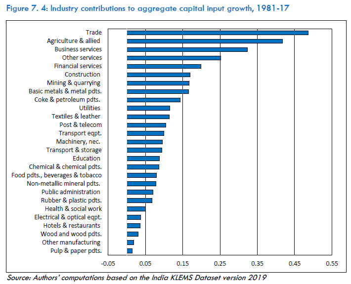 Figure 7.5 provides the ranking of industries in terms of their contributions to aggregate labour input growth. Construction, a predominantly labour-intensive industry, was the largest contributor to aggregate labour input growth. Other leading contributors belong to the Services sector, namely — Other services, Trade, Business services, Transport & storage, and Financial services. While the Agriculture & allied and Education industries made somewhat high contributions, the remaining industries fell substantially behind. In particular, the more labour-intensive industries such as—Textiles & leather, Pulp & paper products, Food products, beverages & tobacco, and Wood & wood products recorded negligible contributions to aggregate labour input growth. Overall, contributions from Manufacturing industries were relatively lower than from Service industries. This reflects the combination of relatively slower employment growth in the manufacturing sector (1.58 per cent) compared with the service sector (3.20 per cent), and a relatively high value-added share of the service sector (45 per cent) compared with a mere 18 per cent share of the manufacturing sector during the period under consideration. 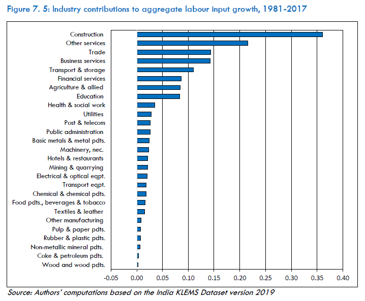 7.5 Disaggregated Growth & Productivity Dynamics – Pre & Post Global Financial Crisis While economic growth and productivity in India have been widely examined in the context of pre- and post-economic liberalisation that began in the early 1990s, we take a different route in this section. It is well known that the 2008 Global Financial Crisis (GFC) had serious implications for the growth path of many economies. What started as deep “fault lines” or global imbalances (Rajan, 2010) resulted in a severe economic crisis for the world economy. Although India’s economic engagement with the world had increased since the 1990s, several factors allowed India to insulate itself from the shocks of the GFC (Joseph, 2009)—a well-capitalised and regulated financial sector, large stocks of foreign reserves and a gradual pace of opening its capital account. However, it is interesting to analyse whether India’s underlying industrial anatomy underwent a change following the GFC. Such analysis is possible by defining the required sub-periods and utilising the industry production accounts developed in this section. For this purpose, we divide the post-1993 period into a pre-crisis period of 1993-2007 and a post-crisis period of 2008-17. We take the financial year 1993-94 as the starting point for this analysis, because the phase of full-scale industrial deregulation started from this point, lasting till 2000-01. This was subsequently followed by the high economic growth phase i.e., 2002-03 to 2007-08. Thus, our pre-crisis sub-period incorporates the phase of systematic economic liberalisation followed by the phase of high growth. The post-crisis sub-period of 2008-17 is usually referred to as a period of global slowdown in productivity growth (Van Ark et al., 2021). To maintain coherency, we present the estimates as per the sequence already followed in the chapter. Thus, we start by exploring the change in sources of output growth, followed by the change in industry contributions to aggregate growth and productivity, and the corresponding industry contributions to the growth of aggregate primary inputs. These changes are estimated by subtracting the annually averaged results for the post-crisis sub-period of 2008-17 from that of pre-crisis sub-period of 1993-07. While the discussion is based on the figures presented, the exact numbers can be seen in Tables 7A.3 to 7A.5 in Annexure 7A. 7.5.1 Changes in sources of output growth, 2008-17 less 1993-07 We observe a heterogenous picture in terms of changes in output growth rates after the global financial crisis. First, we observe a post-2007 acceleration in output growth for 13 out of the 27 industries (Figure 7.6). The industries with the relatively higher increases in output growth were – Wood & wood products, Rubber & plastic products, Education and Transport equipment. Second, there is a notable decline in the performance of some Service industries, particularly Hotels & restaurants and Post & telecom industries. Third, several Manufacturing industries also saw a decline in output growth rate, with notable declines in—Food products, beverages & tobacco at -3.72 percentage points (ppts), Coke & petroleum products (-2.72 ppts.) and Chemical & chemical products (-2.69 ppts.). | After the global financial crisis capital input increased in importance as a source of output growth for 11 out of the 27 KLEMS industries in India, with the largest increase in capital contribution seen in the trade industry | Figure 7.7 ranks the industries according to changes in capital input contribution to their respective output growth, by separating the contributions from capital stock and capital quality.122 It is observed that capital input increased in importance as a source of output growth for 11 out of the 27 industries. Of these, the largest post-2007 increase in capital contribution was seen in Trade at 3.86 ppts., while the corresponding increase in contribution for the rest of the 10 industries ranged from 0.12 to 1.25 ppts. The Agriculture & allied, Mining & quarrying and Utilities industries also experienced an increase in contribution from capital input. The largest deceleration in capital input contribution was experienced by two Services industries, namely — Financial services and Business services. Except for Chemicals & chemical products and Coke & petroleum products, the rest of the Manufacturing industries also saw a deceleration in the contribution from capital input. 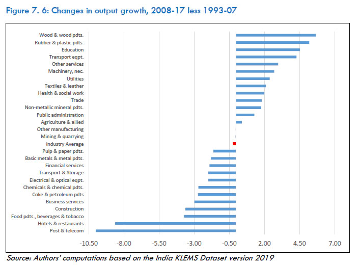 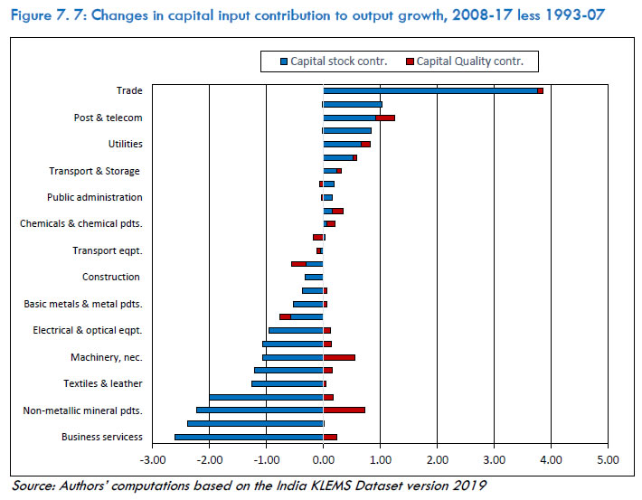 It is also apparent that most of the post-2007 changes in capital input contribution were due to changes in capital stock contribution, rather than capital quality since the former were higher than the latter. Although, an important observation emerges for several industries that saw a post-2007 deceleration in overall capital input contribution—out of 16 such industries, 12 saw a (minor) increase in contribution from capital quality growth. However, the decline in capital stock contribution was overwhelming enough in all these cases, thus decreasing the overall capital input contribution. Looking at the changes in contribution from the second primary input i.e., labour, we observe a rather stark picture (Figure 7.8). The post-2007 changes in contributions from labour input are much less in absolute magnitude compared with the spread in the changes of capital input contributions. Thus, the changes in the former were less volatile for the second sub-period of 2008-17. Except for only four industries—Utilities, Electrical & optical equipment (both registered an increase), Machinery, n.e.c., and Coke & petroleum products (both remained somewhat unchanged), the rest of the 23 industries saw a decline in contribution from labour input for their respective output growth rates.  The largest post-2007 decline in labour input contribution was seen in the Education and the Agriculture & allied industry at -1.08 and -1 per cent, respectively. Much like the preceding discussion on capital input, we find that the changes in labour quality contributions were inconsequential in determing the overall changes in labour input contribution i.e., the employment contribution drove most of the post-2007 changes in contributions of labour input. Figure 7.9 ranks the industries in terms of the change in intermediate input contributions to their respective output growth over the two sub-periods. The change in contributions from the three components of intermediate inputs i.e., Energy (E), Material (M) and Services (S), are highlighted separately to provide a more detailed representation of changes within intermediate inputs. Overall, 14 out of the 27 industries saw a post-2007 increase in contributions from intermediate inputs as a whole (E contr.+M contr.+S contr.). The highest increase in intermediate input contributions came for the Transport equipment, Utilities and Health & social work industries in the range of 3 to 5 ppts. The largest declines among the remaining 13 industries were seen for the Hotels & restaurants and Coke & petroleum products. In the range of -5 to -8. It is also apparent that the majority of the post-2007 changes in intermediate input contributions were caused by the changes in Material input contributions, except for a few cases. 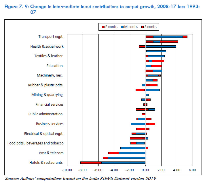 The post-2007 changes in TFP contribution to output growth is shown in Figure 7.10. Given that the second sub-period (2008-17) is characterized by a global slowdown in productivity growth, the following results are important to ascertain which industries were possibly insulated from the negative productivity effects in the aftermath of the GFC. We find a post-2007 resurgence in TFP growth for 15 industries, although at varying rates, while the rest of the 12 industries showed a decline. There are two main observations regarding the type of industries in terms of their post-2007 changes in TFP growth rates – First, capital-intensive industries such as Rubber & plastic products, Non-metallic mineral products, Coke & petroleum products and Basic metals & metal products, saw an increase in TFP growth in the second sub-period; Second, Non-market services such as Education, Other services and Public administration were the second set of industries with a relatively higher post-2007 acceleration in TFP growth. Post & Telecom, Trade, and Chemical & Chemical products were among the sectors that witnessed substantial productivity deceleration. 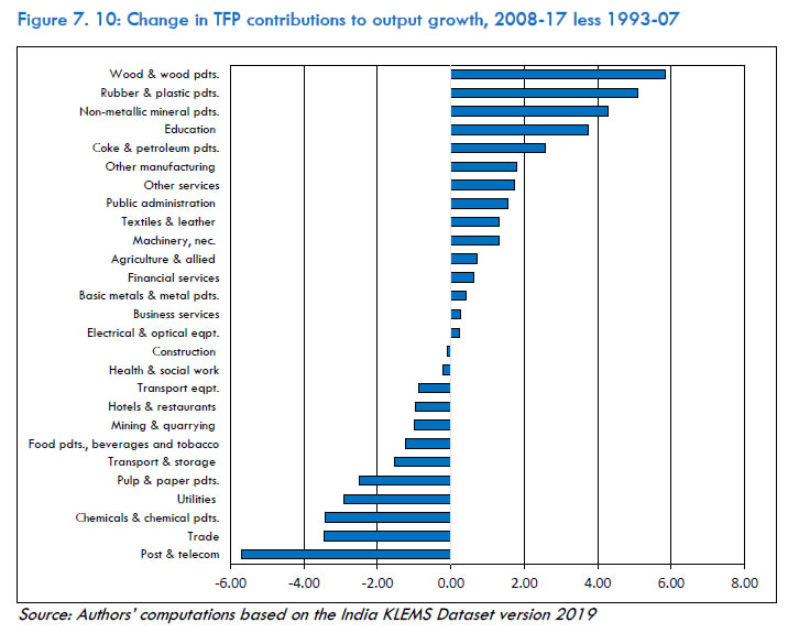 7.5.2 Changes in industry contributions to aggregate growth & productivity, 2008-17 less 1993-07 This section addresses the change in industry contributions to aggregate value-added and aggregate TFP growth over the two chosen sub-periods (by subtracting the annually averaged estimates of CTVA,j and CTTFP,j of 2008-17 from those of 1993-07). Figure 7.11 below provides the ranking of industries in terms of the former. It is observed that 13 out of the 27 industries saw a post-2007 acceleration in their respective contributions to aggregate value-added growth. As shown in Table A.4 of the Annexure, it is found that the annually averaged value-added shares of the industries did not see substantial changes over the two sub-periods. Since CTVA,j (equation (7.14)) is a combination of both industry value-added shares and value-added growth, the changes in contribution over the two sub-periods were thus driven primarily by the respective changes in value-added growth. Among the leading industries, the Coke & petroleum products industry saw the largest acceleration, followed by five Services industries – Business services, Other services, Education, Public administration, and Trade. Among the 14 industries that saw a decline in contribution, the largest decline was observed in Post & telecom, Chemical & chemical products, Transport & storage and Utilities. Notably, the industry with the largest annually averaged value-added share for 1993-17 i.e., the Agriculture & allied industry, saw a decline in its contribution over the two sub-periods. 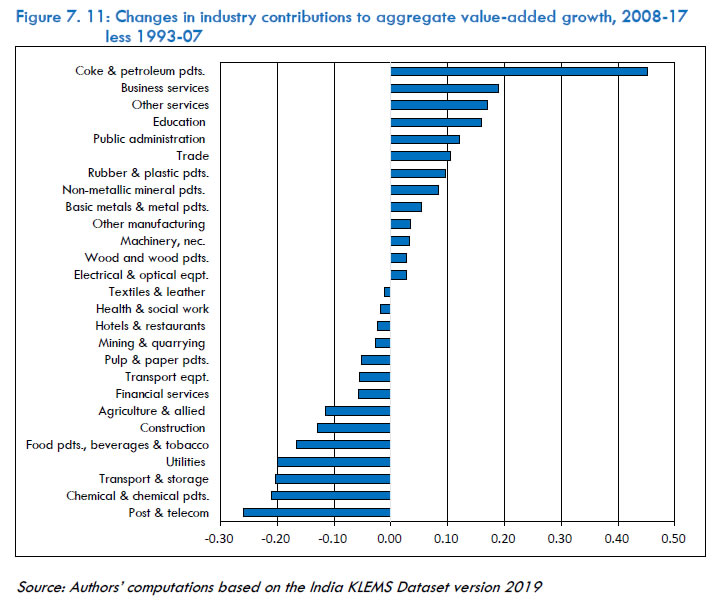 Figure 7.12 provides a similar ranking but in terms to changes in contributions to aggregate TFP growth (CTTFP,j). As seen in Table 7A.4 of the Annexure, it is apparent that although changes industry value-added shares in aggregate value-added were negligible, the Domar weights did see a relatively larger change over the two sub-periods. This indicates that changes in shares of value added by industry in gross output of industry were the primary reason for the changes in the overall Domar weight. We observe that 15 out of the 27 industries saw an increase in their post-2007 contributions to aggregate TFP growth. Notably, the Coke & petroleum industry retained its top spot much like the acceleration in its contribution to aggregate value-added growth. Coupled with the observation of post-2007 TFP growth acceleration in capital intensive industries in Figure 7.10, these industries saw substantial acceleration in their respective contributions to aggregate TFP growth. It is also important to note that out of the 12 remaining industries, several market services registered a decline in their contributions. 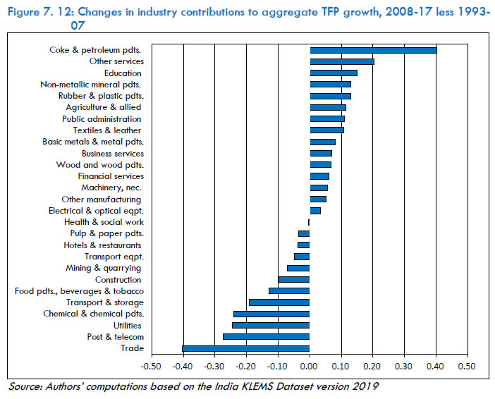 7.5.3 Changes in industry contributions to growth of aggregate primary inputs, 2008-17 less 1993-07 This section deals with the question of change in industry contributions to the growth in aggregate primary input (by subtracting the annually averaged estimates of CTL,j and CTK,j of 2008-17 from those of 1993-07) over the two sub-periods. Figure 7.13 provides the corresponding ranking for industry contributions to aggregate capital input growth. It is observed that the Trade industry saw the relatively largest increase in contribution at 0.59 ppts. From Table 7A.5 in the Annexure, we further find that the associated weights for the Trade industry increased only marginally, and therefore the growth contribution is a result of post-2007 acceleration in capital input growth rate. For the rest of the 12 industries that saw a post-2007 acceleration in their respective contributions, the increases ranged around 0.01- 0.06 ppts. On the other hand, the largest post-2007 decline in contribution was observed for the Financial services (-0.12 ppts.) and Textiles & leather (-0.09 ppts.) industries. These observations could reflect the strong divergence in investment patterns across industry groups in the post-2007 period, and towards a possible substitution of other inputs including labour and intermediate categories for capital input for the 13 industries that saw an increase in contribution to aggregate capital input. 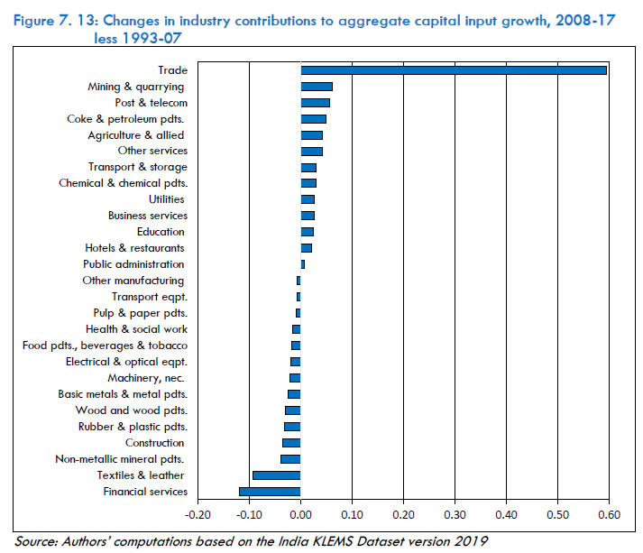 Figure 7.14 provides the ranking of industries in terms of their changes in respective contributions to aggregate labour input growth, over the two sub-periods. As seen in Table 7A.5 of the Annexure, similar to the case of capital input, the associated post-2007 changes in weights for labour input were minor. Thus, the post-2007 changes in labour input growth drove the changes in industry contributions to aggregate labour input growth over the two sub-periods. It is observed that most of the industries (19 out of 27), saw a decline in their post-2007 contributions, with the largest declines observed for the Agriculture & allied (-0.27 ppts.), Trade (0.09 ppts.) and Other services (-0.07 ppts.) industries. On the other hand, the Business services industry (which is mostly skill-intensive in nature) saw the largest increase in contribution of 0.09 ppts. Although the Agriculture & allied industry saw the largest decline in contribution, the largest post-2007 fall in employment growth was observed for the Post & telecom industry at -7.40 ppts (refer to Table 7A.6). Further, the relatively large fall in contribution from the Agriculture & allied industry was a combination of a post-2007 decrease in employment of -2.40 ppts. and the largest fall in weights123 among the 27 industries at -0.03 ppts. 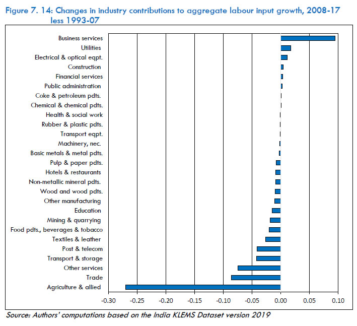 7.6 Sectoral Origins of Growth & Productivity Although we observed significant industry-level heterogeneity in terms of the sources of output growth and contributions to the aggregate economy, for expositional clarity, the 27 India KLEMS industries are aggregated into sectoral and sub-sectoral groups using the appropriate aggregation procedure outlined earlier in equations (7.12) and (7.13). Given the importance of the Agriculture & allied industry as a large employment provider and as an important factor for the sustainability of India’s economic growth (Balakrishnan, 2010), it is covered as a separate sector. Likewise for the Construction, Mining & quarrying and Utilities sectors. The Manufacturing sector is divided into three sub-groups, namely—Manufacturing of Consumer Goods, Manufacturing of Intermediate Goods and Manufacturing of Investment Goods. The Services sector is divided into Market and Non-market sub-groups. As in the preceding sections, we cover the overall period of 1980-2017 and the changes over the two sub-periods of post economic reforms and pre-GFC (1993-07) and the period of post-GFC/global slowdown (2008-17), in order to examine the sectoral dynamics of growth and productivity. Additionally, we present reallocation estimates of labour and capital when discussing the sectoral contributions to aggregate TFP growth, something which was deliberately left out in the preceding disaggregated analysis since the estimates of reallocation do not change when we shift to the sectoral perspective.124 From Table 7.5, we observe that the growth in value added for the aggregate economy during the overall period of 1981-2017 was around 6.12 per cent per annum, while the growth in Manufacturing (8.50 per cent per annum) and Services (7.10 per cent per annum) was higher than the economy average. All three sub-sectors of Manufacturing grew above the economy average, with growth in Manufacturing of Investment goods the highest at around 11 per cent per annum. Accounting for the observed value-added growth (Annexure Table 7A.2 presents estimates on the sources of value-added growth broad sectors from the PPF approach), we find that TFP continues to be a small contributor while capital stock drives much of it. Comparing the Manufacturing sector with Services, we find that capital input and TFP remain the two main contributors to observed growth with a larger absolute contribution by capital stock for the Manufacturing sector relative to Services. Next, we look at the sectoral origins of aggregate value-added growth for the period 1980-2017 by estimating equation (7.12). From the second column of Table 7.5 below, it is observed that the Services sector is the leading contributor (3.20 ppts.) to aggregate value-added growth, followed by the Manufacturing sector (1.51 ppts.). Amongst the Manufacturing sub-groups, the largest contribution comes from the Manufacturing of Intermediate Goods at 0.67 ppts. This sector grew substantially at an average of 8.40 per cent per annum, despite its small share in aggregate value-added at 8 per cent. | Table 7.5: Sectoral contributions to aggregate value-added growth, 1981-2017 | | Broad and Sub-sectors | VA Weights | VA growth | Contributions to Aggregate VA growth | | 1. Agriculture | 0.25 | 3.11 | 0.78 | | 2. Mining | 0.03 | 4.03 | 0.11 | | 3. Manufacturing | 0.18 | 8.50 | 1.51 | | 3.1. Manufacturing of Consumer Goods | 0.06 | 6.80 | 0.41 | | 3.2. Manufacturing of Intermediate Goods | 0.08 | 8.40 | 0.67 | | 3.3. Manufacturing of Investment Goods | 0.04 | 11.14 | 0.43 | | 4. Utilities | 0.03 | 8.65 | 0.24 | | 5. Construction | 0.07 | 3.45 | 0.28 | | 6. Services | 0.45 | 7.10 | 3.20 | | 6.1. Market Services | 0.24 | 7.90 | 1.96 | | 6.2. Non-Market Services | 0.21 | 5.99 | 1.24 | | Aggregate Economy | 1.00 | 6.12 | 6.12 | | Source: Authors’ computations based on the India KLEMS Dataset version 2019 | Impressively, the Investment Manufacturing sub-sector showed the fastest value-added growth of 11.14 percent per annum although its share in aggregate value-added was the smallest at 4 percent, for the overall period. Within the Services sector, the Market services sub-sector showed an almost 2 ppts. higher value-added growth than the Non-Market services sub-sector, even though both had a similar share in aggregate value-added in the range of 20-25 per cent. Overall, value-added growth in most of the sectors was in excess of 5 per cent per annum except for the Agriculture and Construction sector. Figure 7.15 ranks the broad sectors by their change in contributions to aggregate value-added growth from 1993-07 to 2008-17. The three main sectors, namely— Agriculture, Manufacturing and Services, have been highlighted in a different pattern for emphasis. We observe that the Manufacturing sector outperforms the Services and Agriculture sectors in terms of sectoral contributions after 2007. Additionally, it is observed that Manufacturing of Intermediate Goods and the Non-Market Services sub-sectors make the two largest contributions to overall value-added growth after 2007. This increase in contribution is due to the large acceleration in value-added growth after 2007 for both sub-sectors, since their value-added share saw very negligible change post-2007. The rest of the broad sectors saw a post-2007 decline in their respective contributions.125  Moving on to the sectoral contributions to aggregate TFP growth, Table 7.6 presents the estimates from equation (7.13) which are subsequently plugged-in equation (7.11) in order to estimate the reallocation effects. We find that aggregate TFP growth primarily reflects TFP growth from the component industries within the aggregated sectors. The summation of Domar-weighted sectoral contributions to aggregate TFP growth from the 27 underlying industries making up the 6 broad sectors was around 0.96 per cent., while the aggregate TFP growth from the PPF grew at 2.09 per cent per annum. The difference between these figures implies a positive role of reallocation effects of 1.13 per cent in accounting for aggregate TFP growth. The major contributors to the aggregate TFP growth were—Services with a contribution of 0.61 per cent, driven by the 0.42 percent contribution from the Non-market services sub-sector. This was followed by Manufacturing at 0.31 per cent, driven mostly by the 0.13 per cent contribution of the Investment Goods sub-sector. | Table 7.6: Sectoral contributions to aggregate TFP growth, 1981-2017 | | Broad Sectors | Contributions to Aggregate TFP Growth | | 1. Agriculture | 0.28 | | 2. Mining | -0.08 | | 3. Manufacturing | 0.31 | | 3.1. Manufacturing of Consumer Goods | 0.10 | | 3.2. Manufacturing of Intermediate Goods | 0.07 | | 3.3. Manufacturing of Investment Goods | 0.13 | | 4. Utilities | 0.09 | | 5. Construction | -0.25 | | 6. Services | 0.61 | | 6.1. Market Services | 0.19 | | 6.2. Non-Market Services | 0.42 | | Aggregate TFP Growth | 2.09 | | Summation of Domar-weighted sectoral contributions | 0.96 | | Reallocation of Labour | 0.59 | | Reallocation of Capital | 0.54 | | Source: Authors’ computations based on the India KLEMS Dataset version 2019 | The bottom panel of Table 7.6 provides the estimates of the considerable reallocation effects of labour and capital in accounting for aggregate TFP growth. Thus, after accounting for the industry/sectoral contributions, the total reallocation effect is a sum of 0.59 per cent contribution from reallocation of labour and 0.54 per cent contribution from reallocation of capital. As mentioned before, these reallocation effects quantify the departure from the assumption that each type of labour and capital face the same prices in all industries. Since we observe a positive reallocation effect for the overall period of 1980-2017, it can be concluded that different types of capital and labour commanded different prices in the component industries/sectors, and industries/sectors with higher corresponding prices saw higher input growth rates when compared with the economy average. If higher input prices are taken as a reflection of higher marginal productivity (as the assumption of perfectly competitive input markets would imply), it can also be concluded that on an average for 1980-2017, factors shifted to more productive industries/sectors. Figure 7.16 ranks the sectors by the changes in sectoral contribution to aggregate TFP growth from 2000-07 to 2008-17.126 The figure shows considerable heterogeneity in contributions from the main broad sectors and their respective sub-sectors. Notably, the Manufacturing sector shows the largest increase in post-2007 contribution of 0.60 ppts., caused by the large increase in contribution from the Manufacturing of Intermediate Goods at 0.50 ppts. The Services sector’s contribution was driven down to -0.32 ppts due to the large decline in contribution from Market Services (-0.78 ppts.) which outweighed the large acceleration in contribution from the Non-Market sub-sector (0.46 ppts.). The Agriculture sector showed a modest acceleration in contribution of 0.11 ppts, while the Mining and Construction sectors saw a decline in contribution of -0.07 ppts. and -0.10 ppts., respectively. 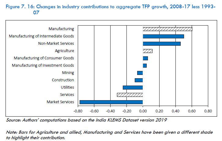 To conclude, Table 7.7 provides the breakdown of aggregate value-added growth into contributions from capital input, labour input and aggregate TFP growth, for the overall period of 1981-2017 and the considered sub-periods of 1993-07 and 2008-17. The sectoral contributions to aggregate value-added and TFP growth have already been addressed and are thus, omitted here. Overall, we find that capital input increased its contribution to aggregate value-added growth in the second sub-period, while the contribution from labour input declined. The change in contribution from aggregate TFP growth over the two sub-periods was negligible. Value-added growth obtained from the PPF approach did not show any substantial acceleration as well. Thus, it appears that the underlying changes in contributions from capital and labour in opposite directions and in nearly equal absolute magnitude combined with negligible change in aggregate TFP growth led to the outcome of little to no acceleration in aggregate value-added growth. | Table 7.7: Decomposition of aggregate value-added growth (PPF), 1981-2017 and sub-periods | | | 1993-07 | 2008-17 | 2008-17 less 1993-07 | 1981-17 | | Value-Added growth | 6.46 | 6.49 | 0.03 | 6.12 | | Contributions | | | | | | Capital Input | 3.84 | 4.39 | 0.55 | 3.61 | | Labour Input | 1.53 | 1.02 | -0.51 | 1.55 | | Aggregate TFP | 1.09 | 1.08 | -0.01 | 0.96 | | Source: Authors’ computations based on the India KLEMS Dataset version 2019 | 7.7 Summary & Conclusions This chapter provides a comprehensive analysis of India’s growth and productivity by examining the disaggregated industry-level production accounts for the 27 India KLEMS industries and six broad sectors that make up the India economy. Growth and productivity dynamics are analysed for the overall period of 1980-2017 and for two sub-periods pertaining to post-systematic reforms/pre-GFC (1993-07) and global productivity slowdown/post-GFC (2008-17). The gross output framework is used to examine the industry-level sources of output growth while the methodologically superior and practically sound Production Possibility Frontier (PPF) approach is used to analyse the origins of aggregate value-added and TFP growth. The limitations of the PPF approach are also addressed by estimating the reallocation effects of labour and capital, which signify a departure from the PPF’s assumption that different types of labour and capital receive the same prices in all industries. Analysis of industry-level output growth rates for 1981-2017 reveals that the output growth rates of 27 India KLEMS industries follow a normal distribution, with the majority of the output growth rates closer to the industry mean of 7.39 per cent per annum. Among the few industries that saw output growth rates higher than the industry mean, the Business services industries saw the relatively highest growth of 12.4 per cent per annum. Decomposition of industry-level output growth for 1981-2017 reveals that intermediate inputs were by far the largest contributors with an industry mean of 4.16 ppts. Within intermediate inputs, most of the contribution was driven by Material (M) input, especially for industries in the Manufacturing sector. Although the contribution from Services input was also substantial for industries such as Agriculture & allied, Utilities and six industries in the Services sector—indicating the importance of intermediate transactions within this sector. Capital input was the second most important contributor, especially for Services industries such as Trade, Business services, and Financial services—indicating high capital intensity in these industries. However, labour input contribution to output growth was very minor, at an industry average of less than one per cent per annum with a few exceptions such as Education and Business services. Given the large workforce in the country, this is a cause for much concern. The quality components of the primary inputs i.e., the contribution from capital and labour quality were marginal for the overall period. However, labour quality was the dominant source of labour input contribution for four industries—Public administration, Wood & wood products, Mining & quarrying, and Agriculture & allied—mostly due to the little to no employment growth in these industries compared with favourable labour quality growth rates, for the overall period. Finally, TFP contribution to output growth (or simply gross output based TFP growth rates) also follows a normal distribution with most of the growth rates near the industry average of 0.47 per cent per annum. The contributions from TFP growth were negligible for most of the industries, except Public administration. However, the estimate of TFP growth in the case of Public administration needs to be interpreted with caution (for reasons given earlier). Overall, for the 1981-2017 period, we observe that input accumulation drove the output growth rates in the Indian economy rather than improvements in efficiency. | Decomposition of industry-level output growth for 1981-2017 reveals that intermediate inputs were by far the largest contributors, with material input as the key driver, followed by capital input | Utilising the PPF approach, we observe that the largest contributors to aggregate value-added growth for the overall period include Agriculture & allied and Services industries—Trade, Other services, Business services and Financial services. While the contribution from the Agriculture & allied sector was largely due to its high share in aggregate value-added (25 per cent per annum), the contributions from the above-mentioned Services industries reflect both, their high shares in aggregate value-added and their high value-added growth. Strikingly, the industries in the Manufacturing sector performed poorly in terms of their contributions. The method of Direct Aggregation across Industries (DAI) allowed the incorporation of the ingenious method of Domar aggregation. From this exercise, we find that the Agriculture & allied and Public administration industries made the largest contributions to aggregate TFP growth for the overall period of 1981-2017. As mentioned before, the case of the latter industry’s TFP growth should be treated with caution. The DAI approach also allowed us to analyse industry contributions to the growth of aggregate primary inputs. For the overall period, this exercise revealed that Service industries were large contributors to aggregate growth of both capital and labour input. The relatively lower contributions from Manufacturing industries towards aggregate labour input growth is again a matter of concern and reflects the poor employment growth in this sector. | Service industries were large contributors to aggregate growth of both capital and labour input. The relatively lower contribution from Manufacturing towards aggregate labour input growth is cause for concern and reflects the poor employment growth. | Looking at the pre (1993-07) and post GFC (2008-17) growth and productivity dynamics, we find widespread revival of TFP growth for 12 industries, mainly those belonging to capital-intensive manufacturing and non-market services. A striking observation is a fall in labour input contribution across the board in the post-GFC period. Indeed, it is hard to attribute this to GFC per se without further scrutiny, but it tends to reflect the economy's inability to create jobs. A post-2007 acceleration in contributions to aggregate value-added growth is observed for five Service sector industries. Whereas a post-2007 acceleration in contribution to aggregate TFP growth is noted for capital-intensive Manufacturing industries, the corresponding contribution from Market services industries saw a decline. The large post-2007 increase in capital input growth of the Trade industry caused a substantial increase in its contribution to aggregate capital input growth in the second sub-period. Finally, it is found that 19 out of the 27 India KLEMS industries saw a decline in their contribution to aggregate labour input growth in the second sub-period, with the largest decline in contributions from the Agriculture & allied and Trade industries. In order to provide an overview of the disaggregated analysis, for expositional clarity, the chapter also undertakes a sectoral analysis of growth and productivity. For the overall period of 1981-2017, although the Manufacturing sector saw higher value-added growth than Services, the relatively higher value-added share of the latter led to a relatively larger contribution to aggregate value-added growth from the PPF approach. Notably, the Service sector contribution to aggregate value-added growth was driven mostly by contributions from the Market services sub-sector. However, the Market services sub-sector saw the largest decline in contributions to aggregate value-added growth over the two sub-periods of 1993-07 and 2008-17. Non-Market services saw a corresponding increase in contribution. The Manufacturing sector saw a substantial increase in its contribution, primarily driven by the large increase in contribution from the Manufacturing of Intermediate goods sub-sector. Finally, we find that aggregate TFP growth for the overall period reflects both TFP growth from the component industries within the aggregated sectors, and positive reallocation effects from labour and capital which occurred at 0.59 and 0.54 per cent, respectively. Similar to the case of sectoral contributions to aggregate value-added growth, over the two sub-periods, we find that Non-Market services sub-sector saw an increase in its contribution to aggregate TFP growth while there was a decline in the corresponding contribution from the Market services sub-sector. Interestingly, the Manufacturing sector saw the largest increase in contribution to aggregate TFP growth—possibly implying that this sector was insulated from the volatility of the post-GFC period. | The Manufacturing sector saw the largest increase in contribution to aggregate TFP growth—possibly implying that this sector was insulated from the volatility of the post-GFC period. | Annexure 7A: Additional Tables | Table 7A.1: Broad and sub-sector classification of 27 India KLEMS industries | | Broad Industry groups | ISIC codes | | 1. Agriculture | Atb | | Agriculture, Hunting, Forestry and Fishing | | 2. Mining | C | | Mining and Quarrying | | 3. Manufacturing | | | 3.1. Manufacturing of Consumer Goods | | | Food Products, Beverages and Tobacco | 15t16 | | Textiles, Textile Products, Leather and Footwear | 17t19 | | Wood and Products of wood | 20 | | Pulp, Paper, Paper products, Printing and Publishing | 21t22 | | Manufacturing, n.e.c.; recycling | 36t37 | | 3.2. Manufacturing of Intermediate Goods | | | Coke, Refined Petroleum Products and Nuclear fuel | 23 | | Chemicals and Chemical Products | 24 | | Rubber and Plastic Products | 25 | | Other Non-Metallic Mineral Products | 26 | | Basic Metals and Fabricated Metal Products | 27t28 | | 3.3. Manufacturing of Investment Goods | | | Machinery, n.e.c. | 29 | | Electrical and Optical Equipment | 30t33 | | Transport Equipment | 34t35 | | 4. Utilities | E | | Electricity, Gas and Water Supply | 5. Construction
Construction | F | | 6. Services | | | 6.1. Market Services | | | Trade | G | | Hotels and Restaurants | H | | Transport and Storage | 60t63 | | Post and Telecommunication | 64 | | Financial Services | J | | Business Services | 71t74 | | 6.2. Non-Market Services | | | Public Administration and Defence; Compulsory Social Security | L | | Education | M | | Health and Social Work | N | | Other services | 70+O+P |
| Table 7A.2: Decomposition of aggregate value-added growth, 1981-2017 | | Broad and Sub-sectors | VA growth | Labour stock contribution | Labour Quality contribution | Capital Stock Contribution | Capital Quality Contribution | TFP Contribution | | 1. Agriculture | 3.11 | 0.00 | 0.17 | 1.57 | 0.22 | 0.78 | | 2. Mining | 4.03 | 0.30 | 0.39 | 5.43 | -0.01 | 2.02 | | 3. Manufacturing | 8.50 | 0.72 | 0.25 | 5.64 | 0.16 | 0.78 | | 3.1. Manufacturing of Consumer Goods | 6.80 | 0.50 | 0.27 | 4.10 | 0.11 | 1.83 | | 3.2. Manufacturing of Intermediate Goods | 8.40 | 0.57 | 0.23 | 6.77 | 0.19 | 0.63 | | 3.3. Manufacturing of Investment Goods | 11.14 | 1.32 | 0.26 | 5.75 | 0.18 | 3.62 | | 4. Utilities | 8.65 | 0.89 | 0.21 | 4.03 | 0.43 | 0.78 | | 5. Construction | 3.45 | 4.77 | 0.31 | 2.24 | -0.01 | 2.02 | | 6. Services | 7.10 | 1.69 | 0.34 | 3.46 | 0.22 | 0.78 | | 6.1. Market Services | 7.90 | 2.04 | 0.25 | 4.58 | 0.24 | 0.78 | | 6.2. Non-Market Services | 5.99 | 1.29 | 0.43 | 2.08 | 0.17 | 2.02 | | Aggregate economy | 6.12 | 1.28 | 0.27 | 3.41 | 0.19 | 0.96 | | Source: Authors’ computations based on the India KLEMS Dataset version 2019 |
| Table 7A.3: Decomposition of changes in sources of output growth, 2008-17 less 1993-07 | | KLEMS Industry Description | Change in Output Growth | Change in Capital Input contribution | Change in Labour Input Contribution | Change in Intermediate input contribution | Change in TFP contribution | | Capital Quality | Capital Stock | Labour Quality | Employment | Energy | Material | Services | | Agriculture & allied | 0.39 | 0.07 | 0.52 | 0.03 | -1.04 | 0.27 | -0.52 | 0.33 | 0.73 | | Mining & quarrying | -0.05 | -0.01 | 1.03 | 0.03 | -0.47 | 0.01 | 0.38 | -0.03 | -0.99 | | Food pdts., beverages & tobacco | -3.72 | 0.05 | -0.36 | -0.02 | -0.21 | -0.13 | -1.08 | -0.73 | -1.24 | | Textiles & leather | 2.10 | 0.05 | -1.25 | -0.04 | -0.35 | 0.30 | 2.12 | -0.04 | 1.33 | | Wood & wood pdts. | 5.67 | 0.18 | -2.01 | -0.01 | -0.87 | 0.09 | 2.49 | -0.03 | 5.83 | | Pulp & paper pdts. | -1.63 | -0.25 | -0.31 | -0.13 | -0.41 | 0.93 | 1.13 | -0.09 | -2.49 | | Coke & petroleum pdts | -2.72 | -0.06 | 0.18 | -0.02 | 0.03 | 0.01 | -4.84 | -0.58 | 2.56 | | Chemicals & chemical pdts. | -2.69 | 0.15 | 0.06 | 0.06 | -0.08 | -0.15 | 1.77 | -1.10 | -3.41 | | Rubber & plastic pdts. | 5.18 | 0.14 | -1.06 | 0.03 | -0.07 | 0.47 | -0.45 | 1.02 | 5.10 | | Non-metallic mineral pdts. | 1.75 | 0.72 | -2.23 | 0.07 | -0.39 | 0.48 | -0.01 | -1.18 | 4.30 | | Basic metals & metal pdts. | -1.80 | 0.06 | -0.53 | 0.01 | -0.08 | -0.45 | 0.32 | -1.55 | 0.41 | | Machinery, nec. | 2.69 | 0.55 | -1.07 | -0.16 | 0.17 | 0.27 | 1.36 | 0.27 | 1.30 | | Electrical & optical eqpt. | -2.00 | 0.13 | -0.95 | -0.03 | 0.26 | 0.12 | -1.23 | -0.53 | 0.24 | | Transport eqpt. | 4.28 | -0.07 | -0.05 | -0.05 | 0.03 | 0.96 | 3.77 | 0.56 | -0.88 | | Other manufacturing | -0.04 | 0.16 | -1.21 | -0.10 | -0.60 | 0.36 | 0.79 | -1.22 | 1.78 | | Utilities | 2.38 | 0.16 | 0.66 | -0.02 | 0.37 | 0.97 | 0.87 | 2.28 | -2.90 | | Construction | -3.61 | 0.00 | -0.32 | 0.03 | -0.32 | 0.01 | -3.21 | 0.27 | -0.09 | | Trade | 1.80 | 0.09 | 3.77 | -0.11 | -0.84 | 0.38 | 0.42 | 1.53 | -3.45 | | Hotels & restaurants | -8.62 | -0.02 | 0.84 | -0.01 | -0.16 | -0.07 | -5.55 | -2.70 | -0.95 | | Transport & Storage | -2.00 | 0.08 | 0.24 | -0.05 | -0.29 | 0.70 | -0.99 | -0.15 | -1.54 | | Post & telecom | -9.99 | 0.33 | 0.92 | -0.02 | -0.82 | 0.06 | -3.38 | -1.38 | -5.70 | | Financial services | -1.91 | 0.01 | -2.39 | 0.03 | -0.13 | 0.14 | 0.06 | -0.26 | 0.63 | | Business services | -2.97 | 0.24 | -2.60 | -0.11 | -0.08 | 0.43 | -1.88 | 0.76 | 0.27 | | Public administration | 1.29 | -0.03 | 0.16 | 0.01 | -0.02 | 0.03 | 0.04 | -0.45 | 1.56 | | Education | 4.52 | -0.18 | 0.02 | -0.16 | -0.93 | 0.07 | 0.65 | 1.31 | 3.74 | | Health & social work | 1.98 | -0.19 | -0.58 | -0.07 | -0.03 | 0.02 | 3.86 | -0.83 | -0.21 | | Other services | 2.97 | 0.19 | 0.15 | -0.03 | -0.55 | 0.04 | 0.84 | 0.60 | 1.74 | | Source: Authors’ computations based on the India KLEMS Dataset version 2019 | Note: The changes in output growth rates are decomposed by the respective components on the right, leading to a net result of zero when the sum of changes in components are subtracted from the respective output growth rates. |
| Table 7A.4: Changes in industry contributions to aggregate value-added and TFP growth, 2008-17 less 1993-07 | | KLEMS Industry Description | Change in VA Shares | Change in VA growth | Change in Industry contributions to Agg. VA growth | Change in Domar Weight | Change in TFP growth | Change in Industry contributions to Agg. TFP growth | | Agriculture & allied | -0.060 | 0.30 | -0.11 | -0.088 | 0.73 | 0.11 | | Mining & quarrying | 0.001 | -0.08 | -0.03 | 0.006 | -0.99 | -0.07 | | Food pdts., beverages & tobacco | -0.001 | -6.98 | -0.17 | 0.016 | -1.24 | -0.13 | | Textiles & leather | -0.003 | 0.60 | -0.01 | 0.003 | 1.33 | 0.11 | | Wood & wood pdts. | -0.003 | 8.05 | 0.03 | -0.005 | 5.83 | 0.07 | | Pulp & paper pdts. | -0.001 | -10.86 | -0.05 | 0.001 | -2.49 | -0.04 | | Coke & petroleum pdts | 0.002 | 41.66 | 0.45 | 0.025 | 2.56 | 0.40 | | Chemicals & chemical pdts. | 0.003 | -10.56 | -0.21 | 0.008 | -3.41 | -0.24 | | Rubber & plastic pdts. | -0.002 | 15.07 | 0.10 | -0.003 | 5.10 | 0.13 | | Non-metallic mineral pdts. | 0.000 | 7.09 | 0.08 | 0.003 | 4.30 | 0.13 | | Basic metals & metal pdts. | -0.003 | 1.73 | 0.05 | 0.020 | 0.41 | 0.08 | | Machinery, n.e.c. | -0.001 | 2.66 | 0.03 | 0.000 | 1.30 | 0.06 | | Electrical & optical eqpt. | 0.001 | -0.54 | 0.03 | 0.007 | 0.24 | 0.03 | | Transport eqpt. | 0.001 | -4.94 | -0.06 | 0.000 | -0.88 | -0.05 | | Other manufacturing | 0.000 | 7.34 | 0.03 | 0.012 | 1.78 | 0.05 | | Utilities | -0.006 | -6.10 | -0.20 | -0.026 | -2.90 | -0.24 | | Construction | 0.018 | -1.94 | -0.13 | 0.046 | -0.09 | -0.10 | | Trade | 0.014 | -0.19 | 0.10 | 0.025 | -3.45 | -0.40 | | Hotels & restaurants | 0.001 | -3.57 | -0.02 | -0.004 | -0.95 | -0.04 | | Transport & Storage | -0.001 | -3.77 | -0.20 | -0.006 | -1.54 | -0.19 | | Post & telecom | -0.002 | -13.05 | -0.26 | -0.004 | -5.70 | -0.27 | | Financial services | 0.009 | -2.28 | -0.06 | 0.012 | 0.63 | 0.06 | | Business services | 0.028 | -3.67 | 0.19 | 0.042 | 0.27 | 0.07 | | Public administration | 0.000 | 2.11 | 0.12 | -0.003 | 1.56 | 0.11 | | Education | 0.006 | 3.47 | 0.16 | 0.010 | 3.74 | 0.15 | | Health & social work | 0.002 | -2.53 | -0.02 | 0.001 | -0.21 | -0.00 | | Other services | -0.005 | 2.05 | 0.17 | 0.000 | 1.74 | 0.20 | Source: Authors’ computations based on the India KLEMS Dataset version 2019
Note: The change in shares/weights multiplied by the change in growth rates will not equal the change in respective contributions since the former’s denominator will be larger than that of the latter due to annual averaging. |
| Table 7A.5: Changes in industry contributions to growth of aggregate primary inputs, 2008-17 less 1993-07 | | KLEMS Industry Description | Change in weights | Change in Capital input growth | Change in Industry contributions to Agg. Capital input growth | Change in weights | Change in Labour input growth | Change in Industry contributions to Agg. Labour input growth | | Agriculture & allied | -0.0254 | 1.57 | 0.04 | -0.0347 | -2.40 | -0.27 | | Mining & quarrying | 0.0021 | 2.77 | 0.06 | -0.0007 | -2.68 | -0.02 | | Food pdts., beverages & tobacco | 0.0001 | -1.31 | -0.02 | -0.0016 | -2.59 | -0.02 | | Textiles & leather | -0.0031 | -4.98 | -0.09 | 0.0004 | -2.89 | -0.03 | | Wood & wood pdts. | -0.0024 | -5.06 | -0.03 | -0.0006 | -6.67 | -0.01 | | Pulp & paper pdts. | -0.0003 | -2.68 | -0.01 | -0.0003 | -3.20 | -0.01 | | Coke & petroleum pdts | 0.0026 | -0.83 | 0.05 | 0.0001 | 0.64 | 0.00 | | Chemicals & chemical pdts. | 0.0028 | 0.44 | 0.03 | -0.0001 | 0.23 | 0.00 | | Rubber & plastic pdts. | -0.0019 | -2.91 | -0.03 | 0.0003 | -1.10 | 0.00 | | Non-metallic mineral pdts. | 0.0004 | -5.09 | -0.04 | 0.0001 | -2.97 | -0.01 | | Basic metals & metal pdts. | -0.0030 | -0.56 | -0.02 | 0.0003 | -0.54 | 0.00 | | Machinery, n.e.c. | -0.0014 | -1.04 | -0.02 | 0.0005 | -0.95 | 0.00 | | Electrical & optical eqpt. | 0.0014 | -5.04 | -0.02 | 0.0001 | 3.20 | 0.01 | | Transport eqpt. | 0.0010 | -1.15 | -0.01 | 0.0002 | -0.55 | 0.00 | | Other manufacturing | 0.0001 | -3.96 | -0.01 | 0.0002 | -4.00 | -0.01 | | Utilities | -0.0074 | 3.78 | 0.03 | 0.0010 | 1.78 | 0.02 | | Construction | 0.0044 | -4.47 | -0.04 | 0.0138 | -1.08 | 0.00 | | Trade | 0.0075 | 10.27 | 0.59 | 0.0064 | -2.36 | -0.09 | | Hotels & restaurants | 0.0003 | 4.86 | 0.02 | 0.0010 | -2.25 | -0.01 | | Transport & Storage | -0.0009 | 1.63 | 0.03 | 0.0000 | -1.65 | -0.04 | | Post & telecom | -0.0027 | 7.16 | 0.06 | 0.0011 | -7.06 | -0.04 | | Financial services | 0.0076 | -4.97 | -0.12 | 0.0010 | 0.07 | 0.00 | | Business services | 0.0145 | -6.19 | 0.03 | 0.0131 | -1.52 | 0.09 | | Public administration | -0.0030 | 2.09 | 0.01 | 0.0027 | 0.00 | 0.00 | | Education | 0.0016 | 0.73 | 0.03 | 0.0047 | -1.61 | -0.02 | | Health & social work | -0.0002 | -2.09 | -0.01 | 0.0020 | -1.10 | 0.00 | | Other services | 0.0054 | 0.13 | 0.04 | -0.0108 | -0.84 | -0.07 |
Chapter 8: Growth, Employment and Labour Productivity in Formal and Informal Manufacturing 8.1 Introduction The analysis of growth in real GVA (gross value added), employment and productivity for the 27 KLEMS industries presented in the previous chapters did not examine the differences in the performances of the formal and informal segments of the industries. This chapter brings this aspect sharply into focus in context of the manufacturing sector. The terms formal and informal manufacturing have been used in literature with varying meanings and coverage. It is, therefore, important to clearly specify how these terms are defined here. The formal segment of manufacturing refers to the organised or registered manufacturing enterprises/establishments. The term ‘registered manufacturing’ has been used in the National Accounts Statistics (NAS) series with base year 2004-05 and its corresponding back series.127 Informal segment naturally means the unorganised or unregistered enterprises/establishments. The terms formal and organised (and accordingly informal and unorganised) are used interchangeably in the chapter. At most places, particularly the sections of the chapter dealing with the presentation of empirical analysis, the terms organised and unorganised are commonly used which adhere to specific, expressed definitions in terms of employment size – this is done to impart greater clarity in the discussion of empirical findings. However, at other places, particularly where the existing literature is reviewed, the terms formal and informal are commonly used – these are used in a more general sense without maintaining rigid adherence to any narrow definitions adopted because the discussion about formality and informality at those places is general and need not be bound by specific definition adopted for the empirical analysis presented in the chapter. There are considerable difficulties in constructing reliable value-added and productivity series separately for the organised and unorganised segments for each of the 27 KLEMS industries. As better availability of data makes it relatively less difficult for manufacturing, the chapter examines this sector. The current National Accounts Statistics (NAS) series (with base 2011-12) provides separate data on GVA for the corporate and household segments of manufacturing industries and the NAS series prior to the 2011-12 series, e.g., the series with base 2004-05, provide data on GVA separately for the registered and unregistered segments for manufacturing industries (i.e. the organised and unorganised segments). Additionally, data on the organised manufacturing are available from the Annual Survey of Industries (ASI)128 and data on the unorganised manufacturing from NSS (National Sample Survey) enterprise surveys. While it is possible to construct time series on GVA for organised (formal) and unorganised (informal) segments (of the 13 KLEMS industries belonging to manufacturing for the period 1980-81 (also referred to as 1980) to 2017-18 (2017), there are difficulties in building a similar series for employment for the entire period. For reasons explained later, the employment series could be formed separately for the organised and unorganised segments of manufacturing only from 1999-2000 onwards. Since consistent employment data are available from 1999-2000 onwards, trends in employment growth have been considered for the period 2000-2001 (2000) to 2017-18 (2017), and two sub-periods, 2000-2007 and 2008-17. Similarly, trends in labour productivity growth are studied for the period 2000 to 2017 and the constituent two sub-periods, 2000-2007 and 2008-17. Since a longer time series is available for real GVA, some analysis of GVA growth at the aggregate level is presented for the period 1981 to 2017 and its four sub-periods, 1981-93, 1994-2002, 2003-07 and 2008-17129, but industry-level analysis of GVA growth is presented for the period 2000 to 2017 and the constituent two sub-periods, 2000-2007 and 2008-17.130 | While it is possible to construct time series on GVA for organised (formal) and unorganised (informal) segments of the 13 KLEMS industries for 1980-81 to 2017-18, the employment series could be formed separately for the organised and unorganised segments of manufacturing only from 1999-2000 onwards. | The chapter is organised as follows. Section 8.2 sets the context in terms of the organised-unorganised segment divide in manufacturing. Section 8.3 discusses the dataset used and methodology adopted for the analysis presented in the chapter. Section 8.4 looks at the share of the manufacturing sector in aggregate economy GVA and employment and the extent of informality in the manufacturing sector. Section 8.5 presents an analysis of trends in growth in real GVA. Section 8.6 looks at employment growth. Trends in labour productivity are taken up for analysis in Section 8.7. This section also goes into the issue of contribution of factor reallocation among industries on aggregate level labour productivity growth and the issue of drag on aggregate level labour productivity growth in manufacturing caused by the unorganised sector. The main findings are summarised, and some concluding remarks are made in Section 8.8. 8.2 Formal-Informal Divide and the Role of the Informal Sector 8.2.1 Formal-Informal Divide in Employment According to International Labour Organization (ILO, 2018a, p.1) “more than 60 per cent of the world’s employed population earn their livelihood working in the informal economy. Informal work exists in all countries, irrespective of the individual country’s level of socio-economic development, but it is far more prevalent in developing countries”. ILO (2014) describes the informal economy being typically marked by high unemployment, underemployment, poverty, gender inequality, and precarious work. Although this segment has become the main source of livelihood for many due to the absence of any entry or exit requirement, it is more a last resort for most. Providing access to some basic income-generating activity that requires relatively little education, skills, technology and capital, the informal economy typically employs workers with low productivity. While some informal activities may offer reasonable livelihoods and incomes, most people “engaged in the informal economy are exposed to inadequate and unsafe working conditions, and have high illiteracy levels, low skill levels and inadequate training opportunities; have less certain, less regular and lower incomes than those in the formal economy, suffer longer working hours, an absence of collective bargaining and representation rights and, often, an ambiguous or disguised employment status; and are physically and financially more vulnerable because work in the informal economy is either excluded from, or effectively beyond, the reach of social security schemes and safety and health, maternity and other labour protection legislation” (ILO, 2014, p3). Since the workers do not have social protection, they find it hard to improve their living standards and come out of poverty. There is, however, much heterogeneity within the informal economy in terms of the various categories of work and the drivers of growth of the informal economy, including informalisation of the formal economy. Despite the substantial attention which ‘informality’ has received, there have been wide variations in its definition both, over time and across countries. One of the first definitions for the informal sector was proposed by Hart (1973). The basis for distinguishing the sectors at this initial stage depended on whether the activity entailed wage earning or self-employment. The 15th International Conference of Labour Statisticians (ICLS) in 1993 defined the informal sector as private unincorporated enterprises producing non-agricultural goods or services meant for sale or barter, with their size—in terms of number of employees—below a certain threshold. According to this definition, informal sector employment comprises all jobs in informal sector enterprises. Note here that while informal sector employment is defined at enterprise level, informal employment is defined at individual or worker level and would therefore also include informal employment in formal sector enterprises. The ILO (2002) later developed a conceptual framework to define the term ‘informal’ sector as one that has “all economic activities by workers and economic units that are—in law or in practice—not covered or insufficiently covered by formal arrangements…”. Since then, different aspects of ‘informalisation’—employment in the informal sector and informal employment, have been identified for different policy prescriptions. While the informal/unorganised sector refers to informal enterprises, informal employment refers to informal jobs. Employment in the informal economy can be defined as the sum of employment in the informal sector and of informal employment found outside the informal sector (formal enterprises and households). In 2003, the 17th International Conference of Labour Statisticians (17th ICLS) adopted “Guidelines concerning a statistical definition of informal employment”131. Based on these guidelines, ILO (2013) defined informal employment as persons employed in the informal sector (including those rare persons who are formally employed in the informal sector) and specifically are: (a) employers in informal enterprises (self-employed); (b) employees in informal enterprises; (c) own-account (self-employed) workers in their own informal enterprises; (d) contributing family workers (self-employed) working in informal enterprises; and (e) members of informal producers’ cooperatives. It further defined persons in informal employment outside the informal sector specifically as (a) employees in formal enterprises not covered by social protection through their work; (b) paid domestic workers not covered by social protection through their work; and (c) contributing family workers working in formal enterprises. | There is much heterogeneity within the informal economy in terms of the various categories of work and the drivers of growth of the informal economy, including informalisation of the formal economy. | Based on the definition of ‘informal employment’, ILO (2018b) provides estimates of informal employment, its composition and magnitude besides other characteristics. In this definition of informal employment, as well as that in ILO (2013) stated above, attention is confined to non-agricultural activities. Table 8.1 provides a summary of the extent of informality in the non-agriculture economy for select developing and BRICS countries and some developed countries. It shows that among the developing countries, the relatively richer countries, e.g., Brazil, Korea, Russia and South Africa have less than half of the persons employed in non-agriculture informal employment, but the informal employment outside the informal sector is one-third in Brazil, Russia and South Africa and one-fifth in Korea (out of total non-agriculture informal employment). On the other hand, the extent of informal employment is more than 50 per cent in the other developing countries—Bangladesh, China, India, Indonesia, and Vietnam with the lowest being 54 per cent in China and the highest in Bangladesh and India at 82 per cent and 78 per cent respectively. However, while Bangladesh has a very high share of informality outside the informal sector (40 per cent), the other countries in this group still have low shares of informality outside the informal sector. This indicates how these countries still depend predominantly on the non-agriculture, informal sector. Among the developed countries, as expected, the share of informal employment in total non-agriculture employment is very low at less than one-fifth (only one-tenth in France), and the maximum share of informal employment comes from the informal sector. Thus, we find that the share of informal employment, generally, depends on the level of development of the country. Also, it seems reasonable to argue that unless the countries with high level of informal employment are able to increase their level of development and adopt suitable policies to reduce informality, it may not be possible for them to succeed in their endevour to reduce informality. | Employment in the informal economy can be defined as the sum of employment in the informal sector and of informal employment found outside the informal sector (formal enterprises and households). |
| Table 8.1: Share of non-agricultural informal employment and its components in non-agricultural employment (latest year available) in developing and developed countries. | | Year | Country | Informal employment | Employment in the informal sector | Informal employment outside the informal sector | | Selected Developing Countries including BRICS | | 2013 | Bangladesh | 82.0 | 49.2 | 32.8 | | 2016 | Brazil | 42.5 | 26.4 | 16.1 | | 2013 | China | 53.5 | 47.3 | 6.2 | | 2012 | India | 78.1 | 64.3 | 13.8 | | 2016 | Indonesia | 80.2 | 62.7 | 17.4 | | 2014 | Korea, Republic of | 28.8 | 23.3 | 5.6 | | 2014 | Russian Federation | 35.6 | 24.3 | 11.3 | | 2016 | South Africa | 34.0 | 21.4 | 12.6 | | 2015 | Viet Nam | 57.9 | 37.4 | 20.5 | | Developed Countries | | 2012 | France | 8.9 | 4.5 | 4.4 | | 2013 | Germany | 10.1 | 9.6 | 0.5 | | 2010 | Japan | 16.3 | 12 | 4.3 | | 2012 | UK | 13.4 | 13.3 | 0.1 | | 2013 | USA | 18.3 | 16.1 | 1.9 | | Source: Compiled from ILO (2018b, Table B1, pp.85-90) | 8.2.2 Informality in India In the context of the growth and development story of India, the informal or unorganised sector has played a very significant role. However, the persisting large share of informal workers in the total workforce132—83.5 per cent in 2017-18 (Natarajan, Schotte and Sen, 2020)— despite rapid growth of the Indian economy since the early 1990s, has puzzled many economists (Raj and Sen, 2016; Bardhan, 2018). This seems to be unique to India as informality has declined in many other Asian countries in recent decades (McCaig and Pavcnik, 2018). Natarajan, Schotte and Sen (2020) find informality in India mostly present among workers who are young, female, less educated, who live in rural areas, and belong to the lower strata of the caste hierarchy. Mehrotra (2019) identifies some demand-side reasons for the persistence of informality as: (i) the pattern of India’s industrial policy in the initial decades of development with reliance on heavy industries and reservation for the small-scale sector, and (ii) labour laws at both central and state levels, which discouraged growth and competitiveness of industry. The most important supply side reason ascribed to informality is the quality of labour supply—low level of education and skill. Sheikh and Gaurav (2020) find from the unit level data for 2011-12 that informality in India could be due to, among other reasons, low level of education, low level of technical and professional training, lack of maternity and childcare support to women, etc. Meanwhile, the recent increase in organised employment is attributed to the rise in wage employment, and some recent policy changes, including the introduction of GST, aimed at formalisation of the economy (Mehrotra, 2019). Unni (2018) however, looks at these policy changes from the ‘capital’ and ‘labour’ perspectives133 and argues that some of the recent policies, e.g., demonetisation and GST might have worked from the capital view, but not much headway has been made from the labour perspective, especially for the manufacturing and the ‘Gig’ economy in blurring the formal-informal divide. | The unorganised sector has been a major contributor to employment and income; Given its prominence in academic discourse, it may be expected there would be consistency in defining the sector in India. However, this was not true till the NCEUS definition proposed in 2009. | In view of the dominance and persistence of informal employment, the rest of this section provides an overview of the organised and unorganised sectors in India, particularly in context of the manufacturing sector. The unorganised sector has been a major contributor to employment and income to the Indian economy for a sustained period of time. This, coupled with the large size of the sector, has made the organised-unorganised divide subject to a large body of literature. Given its prominence in the academic discourse, it may be expected that there would be consistency in defining the sector in India. However, this was not true, till the National Commission for Enterprises in the Unorganised Sector (NCEUS henceforth) proposed in 2009: “The informal sector consists of all incorporated private enterprises owned by individuals or households engaged in the sale and production of goods and services operated on a proprietary or partnership basis and with less than ten total workers.” The term “enterprises” in the above definition includes all workers in the agricultural sector except those in plantations. This is so because workers in the plantation sectors are protected under the Plantations Labour Act, 1951 (Naik, 2009). Such enterprises generally do not fall under the purview of most legislation that governs the organised sector (e.g., for registration of enterprises, and for labour protection). The cornerstone of such legislation, such as labour laws, has been the historical concept of “employment relationship” (ILO, 2003; Chen et al, 2004). The conundrum is that this “employment relationship” is often not defined for the informal sector. The employment relationship may be disguised to avoid falling under the purview of laws. For instance, bidi traders in Ahmedabad claim that they sell tobacco and other related materials to bidi producers. They then buy the bidis from them, thereby avoiding any legal requirements to pay retirement benefits to the bidi producers (Chen, 2006). The definition and basic features of informal sector in India naturally raise questions regarding the linkages it has with the formal sectors of the economy. Ranis and Stewart (1999) show that informal sector produces consumer goods aimed mainly at lower-end customers—goods that often compete with those from the formal sector. Another school of thought contends that the informal sector is integrated with the rest of the economy through complementary linkages (ILO, 1991). Legalists argue that stringent regulations that restrict the organised sector also perpetuate inefficiencies in the unorganised sector134. On the other hand, there is some consensus that the lack of legislation that often characterises most of the informal sector also plays an important role in its perpetuation. The lack of legislation governing street vendors in different Indian cities has often resulted in widespread eviction and bribery (Bhowmik, 2004; Mitullah, 2004). | Legalists argue that stringent regulations that restrict the organised sector also perpetuate inefficiencies in the unorganised sector. However, there is some consensus that the lack of legislation that often characterises the informal sector also plays an important role in its perpetuation. | One common way in which the formal and informal segments of the manufacturing sector interact is through sub-contracting. Many economic relations of production fall somewhere between the two extremes of pure organised and pure unorganised segments. Workers are known to move between points in this spectrum with varying levels of ease and speed (Chen, 2004). For instance, a big garment producing firm may try to reduce its cost of stitching by sub-contracting to small tailors in the informal sector. Likewise, there are many informal enterprises that provide cheap raw materials and labour to the organised segment, thereby making their livelihood contingent on demand from the latter. This is especially true for Indian manufacturing—increasing competition due to openness increases the pressure to reduce costs. This, along with strict labour regulations, provides an ideal scenario for extensive sub-contracting (Mazumdar and Sarkar, 2008; Ramaswamy, 1999). There are two contending views about the nature of sub-contracting. In the stagnation view, formal enterprises subcontract to informal labour-intensive units to minimise their labour costs (Portes, 2004; Tokman, 1978). This results in a vicious cycle of worsening labour conditions and downward pressure on wages. On the contrary, the modernisation view sees sub-contracting as a vehicle for modernisation of the unorganised sector, where formal enterprises establish sub-contracts with informal enterprises capable of using modern technology to ensure minimum standards in quality (e.g., Ranis and Stewart, 1999; Marjit, 2003). Moreno-Monroy et al, (2012) adheres to the latter view by showing a significant positive relationship between organised sector subcontracting and total employment in the relatively modern segments of the unorganised sector. However, they also find evidence of rapid growth of the relatively traditional segments of the unorganised sector as well. One possible reason for this is the take-over of the more labour-intensive industries by these traditional segments. Other possible reasons include strict labour laws governing the organised sector (Besley and Burgess, 2004) and structural production links between the organised and unorganised segments (Aghion et al, 2008). | One common way in which the formal and informal segments of the manufacturing sector interact is through sub-contracting. Many economic relations of production fall somewhere between the two extremes of pure organised and pure unorganised segments. | As the formal-informal divide is most prominent in the manufacturing sector (WTO, 2009), there are quite a few studies (Goldar, 2000; Kannan and Raveendran, 2009; Krishna et.al., 2018; etc.) that focus on these aspects. India’s manufacturing sector has undergone significant transformation since Independence. Under the first three Five Year plans (1951-65), it witnessed rapid growth (around 8 per cent p.a.) and diversification under the import-substitution regime. After a period of stagnation in industrial growth, India initiated a series of economic reforms in the 1980s and further liberalisation following the crisis of 1990 to promote competitiveness and efficiency in the Indian manufacturing sector, with the objective of attaining a higher economic growth trajectory. However, the structure of the manufacturing sector—comprising a substantive informal segment with relatively less-productive enterprises135 has affected the growth performance despite the economic liberalisation. This is also reflected in the growth rate of value added in each of the segments. The growth rate of total manufacturing has been increasing in each decade for the period 1980-2011, with the formal segment growing faster than the informal. The pattern has been somewhat different in case of employment trends. The annual growth rate of employment in total manufacturing was around 2 per cent during 1980-99, with growth in the unorganised segment being higher at 2.54 per cent, than the formal segment, which registered a mere 0.23 per cent growth in employment (Annexure 8.3, Table A8.2). But in the subsequent period of 2000-17, it is the growth in employment in the organised sector, 2.72 per cent, which outpaced the informal sector where employment grew by just 0.46 per cent. | Manufacturing employment grew at 2 per cent in 1980-99, with growth in the unorganised segment higher (2.54 per cent) than the formal (0.23). But in 2000-17, growth in employment in the organised sector at 2.72 per cent outpaced that in the informal segment (0.46 per cent). | 8.3. Dataset and Methodology 8.3.1 Data The basic source of data used in the current chapter is the India KLEMS database, 2019. The data is consistent with India’s national accounts. The KLEMS database includes, among other variables, data on value added, at both current and constant prices, and for employment for aggregate manufacturing and its 13 constituent industries. However, data for the organised and unorganised segments has been computed by using the methodology outlined in the next section. 8.3.2 Methodology In this section, we discuss the methodology for computing (a) employment for organised and unorganised sectors, (b) gross value added for the organised and unorganised sectors, and (c) labour productivity for the 13 industries in the Indian manufacturing sector. We also outline the procedure used to find the (d) drag on labour productivity due to informality in the sector, as well as (e) the decomposition method to ascertain the within-industry productivity growth component and the component representing the contribution of structural change among the industries towards aggregate level labour productivity growth. (a) Construction of employment series for organised and unorganised segments Two possible approaches may be taken for constructing employment series for organised and unorganised manufacturing. One possible approach involves the following steps: (1) take the total employment in each of the 13 manufacturing industries from the India KLEMS database, 2019 (which is based on results of the NSS employment-unemployment survey (EUS) and periodic labour force survey (PLFS) as explained in the chapters dealing with database construction and labour input), (2) take employment data for organised segments of the 13 manufacturing industries from ASI, and then (3) derive the employment in the unorganised segments as the residual (with appropriate modifications). Krishna et al. (2018) has adopted this approach. A second possible approach is to use the EUS and PLFS data directly to obtain estimates of employment in the organised and unorganised segments of the 13 KLEMS manufacturing industries (consistent with the employment series in the India KLEMS database 2019). One limitation of the first approach is that there may be some problems of comparability between the data on employment obtained from EUS/PLFS and those obtained from ASI. Therefore, the second approach is preferred and has been adopted for this analysis. Using the second approach, the organised and unorganised sector components from the EUS are estimated with the help of the questions related to enterprise type and the number of workers it employs. This chapter follows the approach detailed in Sundaram (2008) about the categories to be included under ‘organised sector’136. According to Sundaram, as per 1999-2000 EUS, organised sector employment which conforms to the organised sector coverage of NAS includes all workers “working in enterprises in the public sector (code 5 of enterprise type in EUSs), in semi-public enterprises (code 6), and others (including cooperative society, public limited company, private limited company and other units covered under Annual Survey of Industries (ASI) (code 7))”. For the 61st EUS and 68th EUS, some units covered under ASI are not separately coded, so the information is obtained by identifying such enterprises through the response on the ‘use of electricity’ and the ‘number of workers employed’. Workers employed in any enterprise, which has employed more than 10 workers and is using electricity or employs more than 20 workers without using electricity are included in organised sector employment. Using the definition, employment for all 13 manufacturing industries has been computed from the unit level data released by NSS for different rounds starting from 1999-2000 and PLFS (2017-18). We start from 1999-2000 because NSS began identifying characteristics of informality of sectors only from that year in its 55th round of the Employment and Unemployment Survey (EUS). Consistent and reliable information on organised and unorganised employment can be obtained from EUS only from 1999 onwards. | This chapter has adopted the approach of using EUS and PLFS data directly to estimate employment in both organised and unorganised segments of the 13 KLEMS manufacturing industries. This has been done with the help of questions related to enterprise type and number of workers. | (b) Construction of real GVA Series for organized and unorganized segments Annexure 8A details how the real GVA series has been constructed for the organised and unorganised segments of the manufacturing industries. In brief, the series are first constructed at current prices and then deflated to obtain the series at 2011-12 prices. The implicit deflators for GVA series for the 13 manufacturing industries in the India KLEMS database 2019 have been used here. The series at current prices for the organised segment was constructed first for each industry for the years 1980 to 2011. Then, for each industry, a series on GVA at current prices was formed on the basis of ASI data for the years 1980 to 2017. The former series, available till 2011, was then extended to 2017 with the help of the series prepared using ASI data (using the regression technique). Having obtained the GVA series for the organised segment, then, that for the unorganised segment has been derived as residual. Certain problems were encountered when this method was applied in the case of one of the industries, namely ‘coke, refined petroleum products and nuclear fuel’. For that industry, a slightly different method has been applied for obtaining estimates of GVA at current prices for organised and unorganised segments for the years 2011 to 2017, as explained in Annexure 8A. (c) Computation of Labour productivity Labour productivity (LP) for the aggregate manufacturing sector is defined as real gross output per unit of person employed. Using the notations and broadly the methodology used by Djidonou and Foster-McGregor (2020), LP (yt) is defined as where VAt is total value added (real) and Lt is total employment. Since manufacturing consist of 13 industries, therefore the aggregate labour productivity can also be defined as the weighted sum of the 13 individual LPs (yit), with weights being the employment share of each industry (sit) in total manufacturing employment at time t. Hence, we may write However, if we divide the aggregate manufacturing into organised and unorganised segments, then aggregate labour productivity will be equal to the weighted labour productivity of the organised and unorganised segments with weights being the respective employment share of the two segments. Then, we may rewrite aggregate labour productivity, yt as follows137 (d) Computation of drag due to informality So, while the first term in equation 8.3 refers to the productivity level of the aggregate manufacturing sector in the absence of informality, the second term is the cost due to the presence of informality and is expected to be negative, as labour productivity in the unorganised segment of an industry is expected to be lower than in the organised segment. If we differentiate equation (8.3) with respect to time, we may obtain the drag on the aggregate labour productivity growth of manufacturing due to the presence of the unorganised segment as follows: One may notice from equation 8.4 that the extent of the drag depends on the difference between the labour productivity of the unorganised and the organised segment, and on the share of the former within the sector (industry). So, the cost will be small if either one or both are small in magnitude. Since, the share of informality within an industry is high in developing countries, therefore the drag due to informality is also higher as compared to developed countries where the share of informality is low. (e) Decomposition of labour productivity- within and between effects We next describe how we study the contribution of structural change to growth in aggregate labour productivity for the 13 industries of the Indian manufacturing sector, further decomposing it into organised and unorganised segment contribution. We use decomposition methods to understand the contributions of structural change to aggregate level factor productivity growth. The method applied for this purpose can be traced to the shift-share decomposition of Fabricant (1942) and later the methodology proposed and applied in the study by Baily, Hulten and Campbell (1992) in context of manufacturing plants, which was subsequently modified by Haltiwanger (1997). The decomposition method is widely used to decompose the growth rate of aggregate factor productivity growth into a within industry productivity growth component (also known as intra-sectoral effect) and a ‘between effect’, also known as reallocation, shift or structural change effect. It is thus the ‘between effect’ which is used as a measure of structural change by researchers (e.g., OECD, 2013; Ghani, 2013; Goldar and Aggarwal, 2015; Goldar, et al., 2017). Using the decomposition methodology that was applied recently by Djidonou and Foster-McGregor (2020), the annual change in labour productivity levels is decomposed into within industry productivity change component and a structural change component: In the above equation, yi is the labour productivity in industry i and si is the employment share of industry i in aggregate employment, and the symbol Δ indicates change over the previous year. The first term in equation (8.5) is the within effect, or the effect of productivity change within the organised and unorganised segment of each industry. It denotes for each industry the sum of change in productivity levels weighted by its respective employment share in the previous period. The within manufacturing sector component captures not only intra-sectoral reallocation but also the technological and institutional improvements that might happen within the manufacturing sub-sectors. The second term is the between effect or structural change—a measure of the effect traceable to workers reallocation across industries—that is calculated by a change in employment weighted by levels of productivity. If it is positive, it suggests that workers move to sectors with above-average productivity levels, and this term is often considered as a static reallocation (or static between) effect and is also described as the structural-change term measuring the movement of workers from less productive to more productive industries. Finally, we obtain the decomposition of labour productivity growth rates by dividing both sides of the equation by aggregate labour productivity in the previous period. By incorporating the organised -unorganised segment distinction to the standard shift-share decomposition, it has become possible to identify the contributions of the organised and unorganised segments to the within and structural change effects on labour productivity growth. The extension of the decomposition analysis helps us to find and understand how the structural change components of aggregate labour productivity growth are driven by structural change within the organised and unorganised segments or by movements between the two segments. The structural change component (SC) of the equation (8.5) can be rewritten as below, by rearranging the terms after adding and subtracting the two terms Sj,t SFj,t-1yFj,t and Sj,t SI j,t-1 yI j,t. 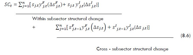 Equation (8.6) decomposes the structural change component into within and between segment labour reallocations. The first term on the right-hand side of Equation (8.6) expresses the impact of the workers (re)allocation within sub-sectors (13 manufacturing industries) of organised and unorganised segments. As such, this term will be non-zero if there are movements between the two segments within the subsectors. A negative value of the component implies that workers move, on average, from the more productive organised segments to the less productive unorganised segments within sub-sectors, and vice versa for a positive value. The second term on the right-hand side of Equation (8.6) indicates movement of workers across sub-sectors. This additional decomposition, therefore, allows us to examine whether the structural change component of labour productivity growth is driven by movements between organised and unorganised segments within sub-sectors or by the movement of workers across subsectors. 8.4 Relative Share of the Manufacturing Sector and the Extent of Informality While this section focuses on informality in the manufacturing sector in India, it is useful to begin the discussion by looking at the inter-temporal trends in the relative share of the manufacturing sector in real GVA and employment in the Indian economy. This is done in Section 8.4.1, which is followed by a discussion on informality in the manufacturing sector in Section 8.4.2. 8.4.1 Manufacturing sector Since the beginning of the industrial revolution in Britain, manufacturing has been considered the main engine of economic growth and development and structural change was linked with the shift of resources primarily from traditional agricultural sector to the manufacturing sector. Kaldor (1967) sought to empirically explain the economic development of Western Europe on the basis of the manufacturing sector, which he argued was the engine of growth for every country at every stage of economic development. Kaldor posited that: increasing returns in the manufacturing sector mean faster growth of manufacturing output which is associated with faster economic growth. This is because backward and forward input–output linkages are strongest in manufacturing, and the scope for capital accumulation, technological progress, economies of scale, and knowledge spill-over is strong. Further, there is a strong causal relationship between manufacturing output growth and labour productivity because of a deepening division of labour, specialisation and learning-by-doing, and the scope for productivity gains is large due to economies of scale. Rodrik (2013) shows that increasing returns to scale imply that as costs fall, demand rises for manufacturing goods (high-income elasticities of demand), triggering more manufacturing and higher incomes, more demand, and cost reductions. Many studies (Szirmai, 2009; Trgenna, 2007; Kathuria and Natrajan, 2013) also find that industrialisation has played an important role in economic development and a few others (Attiah, 2019; Rodrik, 2009) find support for the important role of structural transformation in periods of growth acceleration. The East Asian experience and other historical examples of economic development have been associated with successful industrialisation (Szirmai, 2009). Haraguchi, et.al. (2017) find evidence of manufacturing continuing to play a key role in the growth of developing countries even after 1990 and conclude that its role will likely remain important for low-income countries in the future. A similar conclusion is reached by Cantore, et. al. (2017) in a study covering 80 countries for the period 1980-2017. However, Szirmai (2009), based on 50 years of data for 63 developing and 16 developed countries, found that manufacturing acted as the ‘engine of growth’ during 1950-73—and more so in developing countries than in advanced countries. After the 1970s, the massive spurt in ICT technology benefited the service sector more, leading to it expanding faster than the manufacturing sector. Dan and Yao (2017), however, also found support for manufacturing as an engine of economic growth in middle-income countries and observed that ‘in the middle-income stage, manufacturing pulls along all the other sectors, including the services sector and a larger share of manufacturing promotes the private saving ratio and accelerates the pace of technological accumulation’. | While this section focuses on informality in the manufacturing sector in India, it is useful to begin the discussion by looking at the inter-temporal trends in the relative share of the manufacturing sector in real GVA and employment in the Indian economy. | Based on theoretical and empirical evidence, four underlying factors accounted for the importance of manufacturing in economic growth: (i) it is a source of capital accumulation (Szirmai, 2009), (ii) it offers greater opportunities of economies of scale (Kaldor, 1967), (iii) it is a source of advancement in technology (Cornwall, 1977), and (iv) it offers stronger backward and forward linkages (Dan and Yao, 2017) and spill over-effects between different sectors—so higher productivity in manufacturing sector than in agricultural sector induces transfer of resources, especially labour from agriculture (Dan and Yao, 2017). While Mehrotra (2020) reiterated these important contributions of manufacturing, Sharma (2020, pp.12) mentioned that manufacturing generally has the biggest impact on the direction of the economy, because it has traditionally been the main source of jobs, innovation and increases in productivity. It is also asserted by many studies (Rodrik, 2013; Panagariya, 2008; Acharya et al., 2003) that for a developing country like India, it is important to maintain a high manufacturing growth without which the pace of growth of the service sector cannot be sustained—and except for a few countries with abundant natural resources, almost all countries that sustained a high growth did so with the help of the manufacturing sector (Rodrik, 2013). | Advanced economies are now predominantly service economies, and experiences of India and other emerging economies raise the question whether services have become the key sector in economic development in the twenty-first century. | However, the consensus in the old economic literature that manufacturing was the key to economic development is now questioned because advanced economies are now predominantly service economies, and the recent experiences of India and other emerging economies raise the question whether services have become the key sector in economic development in the twenty-first century (Szirmai, 2011). The new economic literature (Timmer and de Vries, 2007) confirms the increase in importance of the service sector and shows that in advanced countries, service sectors now account for over two-thirds of GDP. This alone gives the service sector substantial weight in economic growth. The developing countries are also now characterised by a very large share of the service sector even at an early stage of development. Many of them did not follow the traditional linear sequence of a shift from agriculture to manufacturing, and a subsequent shift to services. There is evidence now, which suggests that even as deindustrialisation138 has taken place in the developed world (Rodrik, 2015), manufacturing is no longer growing even in the developing world. Rodrik (2015) finds evidence of an ‘inverted U-shape’ curve for manufacturing where its share first rises and then tends to fall over the course of economic development. Countries have reached ‘peak manufacturing’ in employment and value-added shares at a much earlier point139 than the advanced nations in terms of income per person and are experiencing ‘premature deindustrialisation’ (Palma, 2005 and Rodrik, 2015). The deindustrialisation is more visible in the share of manufacturing in employment rather than that in output. The developing countries are peaking in manufacturing employment at lower income levels and the shares in total employment are lower than in the past (the peaking has been taking place in the recent times at below 18 per cent as compared with over 30 per cent in the past according to Felipe, et.al., (2015)). Two important reasons account for this phenomenon, (i) trade liberalisation and internationalisation of supply chains that have increased international competition (Rodrik, 2015, Felipe, et.al., 2015), thus forcing many of the factory jobs to move to the low wage countries which also happen to be less-productive countries140 and (ii) technological change that is labour saving. Many studies (Rodrik, 2015, Felipe, et.al., 2015, Haraguchi, et.al., 2017), however, find very little change in the manufacturing sector’s value-added and employment shares in world GDP and employment during the last 40 years because of a shift of manufacturing to relatively more populous and less developed countries, which led to a concentration of manufacturing activities in these countries. | Developing countries are peaking in manufacturing employment at lower income levels and the shares in total employment are lower than in the past. | Palma (2005) gives several other potential hypotheses that could explain the phenomenon: (i) contracting out of manufacturing jobs to services (for example, cleaning, catering, security, logistics, accounting, etc); or (ii) a fall in the income elasticity of manufactures; or (iii) higher productivity growth in manufacturing; or (iv) global outsourcing that resulted in a fall in manufacturing employment or (v) technological progress. Nayyar et.al. (2018), however, attributes premature deindustrialisation more to the similar features of many services sectors as of manufacturing e.g., scale economies, exports, and innovation. The authors, however, also acknowledge that the skill set required for most service sectors, e.g., ICT, communication services, etc. may be different from the manufacturing sector and may not simultaneously create jobs for the same set of labour. Rodrik (2015) highlights that the consequence of deindustrialisation is service-led growth. He, however, points out (p.24) that ‘many services, such as IT and finance, are high productivity and tradable, and could play the escalator role that manufacturing has traditionally played. However, these service industries are typically highly skill‐intensive, and do not have the capacity to absorb—as manufacturing did—the type of labour that low‐ and middle‐income economies have in abundance. The bulk of other services suffer from two shortcomings. They are either technologically not very dynamic, or non‐tradable, which means their ability to expand rapidly is constrained by incomes (and hence productivity) in the rest of the economy’. Turning now to India, manufacturing in India occupied a key role in Indian development planning from the beginning of the Second Five Year Plan in 1956, and heavy industries, especially in the public sector were provided a key role. Manufacturing in India acted as the engine of growth in the early 1970s and 1980s and only slowed after the economic reforms of the 1990s as it was input-driven instead of efficiency-driven (Kalirajan, and Bhide, 2005). Kathuria and Natrajan (2013) find that despite a decline in its share, manufacturing acted as the engine of growth in the post-1990s and was driven mainly by factor accumulation rather than productivity growth. Sarkar (2015), on the other hand, finds that manufacturing in India did not play its historical role in reallocation of output and employment from agriculture. Nagaraj (2021) points out that though India did not face deindustrialisation,141 but experienced stagnation between 1991 and 2016 with a share of only 14-15 per cent in GDP as compared with a higher (generally 30 per cent) share in many other Asian economies. | Between 1999 and 2017, while there was a slight increase in the manufacturing sector’s share in real value added at the aggregate level from 15 to 18 per cent, it remained stagnant at 11 per cent in aggregate employment. | Figure 8.1 shows that between 1999 and 2017, while there was a slight increase in the manufacturing sector’s share in real value added at the aggregate level from 15 to 18 per cent, it remained stagnant at 11 per cent in aggregate employment. This may be contrasted with the services sector which experienced an increase of 10 percentage points in its share in both GVA and employment between during the same period, 1999-2017. Given the stagnant share of manufacturing in employment, the phenomenon has been termed as ‘jobless growth’.142 Though the total number of persons employed in manufacturing increased by almost 10 million during 1999-2017, the figure fell by 2 million persons between 2011-12 and 2017-18. Figure 8.1: Share of manufacturing sector in value added and employment in the economy 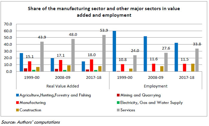 Dhawan and Sengupta (2020) suggest that Indian manufacturing could still become an engine of both economic growth and jobs if it can specialise in and participate in global value chains of the 11 sectors where it has a comparative advantage. They argue that it can be done, among other things, by focussing on four market opportunities: export growth, import substitution with localisation, domestic demand, and contract manufacturing. They advocate appropriate policy interventions, such as, (i) raising the productivity of labour and capital with better infrastructure, logistics, product quality, branding, and packaging, (ii) accessing capital—domestic and foreign, and (iii) getting know-how and technology. Gandhi and Chaudhary (2020) have also argued that India can become a global manufacturing hub and compete with China if its competitiveness is enhanced with reforms related to infrastructure, logistics, labour, land, contract enforcement, and dispute resolution, etc. Mehrotra (2020) attributes the stagnation in manufacturing to the absence of a coherent industrial policy since 1991 and argues for an appropriate strategy to address the concerns of all enterprises—large, small and medium, and micro. Suresh (2017) highlights the importance of high technology industries in Indian manufacturing, while discussing aerospace, pharmaceuticals, and automotive, as India’s successes and telecommunication equipment as an unsuccessful case. Chanda (2018) emphasises the importance of interdependence between the manufacturing and the services sector, while designing any policy to boost manufacturing. While thinking about India’s manufacturing sector and the role it may play in India’s economic growth in coming years, it is important to recognize that it has a dualistic structure with the prevalence of organized and unorganized sectors. Though the share of unorganized sector in employment is still large, but it has declined in the recent period. The increase in manufacturing employment between 1999 and 2017 has been observed more in the organized sector (7 million) than in the unorganized sector (3 million). Thus, the growth in employment in the manufacturing in the unorganized sector remained stagnant. This is taken up for further discussion in the following section. 8.4.2 Informality in the manufacturing sector of India Our study finds that informality in India’s manufacturing is not only dominant but is also persistent. Table 8.2 shows that while the unorganised sector contributes only one-third to the total manufacturing value added in both 1999-00 and 2017-18, its share in total employment in manufacturing is more than 60 per cent despite declining during this period. In absolute terms, an additional 2.6 million persons were employed in the unorganised sector during this period, out of an overall increase by nearly 10 million persons in total manufacturing employment. Organised sector employment is only 34 per cent of the total manufacturing employment in 2017-18. We notice however, that there is a lot of variability in the degree of informality among the 13 manufacturing industries in India and the two shares are not uniform. On the one hand, the share of unorganised sector in both, total value-added and employment is more than 90 per cent in Wood and Wood Products throughout 1999-2017, and on the other hand share in value added is almost nil for the Coke and Petroleum Products industry despite a substantial 26 per cent share in employment in 2017. The reason is that the employment in the unorganized sector of the industry relates to substantive casual labour. The dominance of the unorganised sector in employment (80 per cent or more) is evident in the traditional labour industries (sub-sectors of manufacturing) of Food Products, Beverages and Tobacco, Textiles and Leather, Wood and Wood Products, and Other manufacturing (Manufacturing n.e.c.; recycling), and it is less prominent (less than 35 per cent in 2017) in the non-traditional industries of Coke and Petroleum Products, Chemicals and Chemical Products, and Transport Equipment. Promotion of these non-traditional industries may help in ‘formalisation’ of the manufacturing sector. India, therefore, needs sector-specific industrial strategies, alongside approaches for addressing the general problems of poor infrastructure, uncertain electricity supply, access to credit, etc. | Table 8.2: Percentage share of unorganized sector in total manufacturing in value added and employment | | Industry | Real Value Added | Employment | | 1999-00 | 2008-09 | 2017-18 | 1999-00 | 2008-09 | 2017-18 | | All Manufacturing | 33.9 | 28.0 | 33.5 | 74.5 | 68.2 | 66.0 | | Food Products, Beverages and Tobacco | 51.0 | 38.0 | 33.4 | 81.2 | 79.3 | 79.0 | | Textiles, Textile Products, Leather and Footwear | 65.5 | 58.0 | 58.0 | 78.2 | 70.4 | 68.7 | | Wood and Products of wood | 95.8 | 95.2 | 92.2 | 97.7 | 95.6 | 91.3 | | Pulp, Paper, Paper products, Printing and Publishing | 46.9 | 37.0 | 28.7 | 65.9 | 58.5 | 61.0 | | Coke, Refined Petroleum Products and Nuclear fuel | 0.7 | 0.3 | 0.1 | 22.7 | 17.9 | 26.1 | | Chemicals and Chemical Products | 15.8 | 11.7 | 21.8 | 45.2 | 29.3 | 28.8 | | Rubber and Plastic Products | 20.0 | 26.1 | 33.3 | 45.5 | 41.9 | 33.5 | | Other Non-Metallic Mineral Products | 46.0 | 34.9 | 50.1 | 73.5 | 59.4 | 61.3 | | Basic Metals and Fabricated Metal Products | 24.7 | 25.4 | 31.1 | 64.4 | 59.1 | 60.5 | | Machinery, n.e.c. | 24.7 | 16.1 | 13.7 | 47.5 | 42.9 | 52.2 | | Electrical and Optical Equipment | 22.2 | 19.6 | 32.5 | 30.5 | 56.5 | 61.8 | | Transport Equipment | 18.8 | 17.6 | 40.4 | 28.3 | 21.5 | 32.3 | | Manufacturing, n.e.c.; recycling | 68.2 | 78.0 | 75.2 | 85.7 | 79.0 | 78.0 | n.e.c.= not elsewhere classified.
Source: Authors’ computations | 8.5 Growth in Real GVA, Organized and Unorganized Manufacturing This section presents a comparative analysis of real GVA growth in the organised and unorganised segments of 13 manufacturing industries. It also analyses patterns for the periods 1980-2017, and 1999-2017 in alignment with the periods selected for analysis in subsequent sections of the chapter. Table 8.3 shows that during 1981-2017, the average annual growth rate in real GVA in total manufacturing (industry-wise details are provided in Annexure Table 8B.1) was about 6.7 per cent, while it was 7.2 per cent for organised manufacturing and about 6 per cent for unorganised manufacturing. On examining the sub-periods, the growth rate in real GVA in organised manufacturing (7.6 per cent) significantly exceeded that in unorganised manufacturing (3.6 per cent) during 1981-93, i.e., the pre-reforms period. This gap in growth rates in real GVA narrowed down significantly in the next sub-period, 1994-2002, but widened once again during 2003-07, a period of high growth in the Indian economy. Interestingly, during 2008-17, the sub-period bearing the impact of global economic slowdown, it was unorganised manufacturing that registered a higher growth in real GVA than the organised segment. While there was a marked slowdown in the growth rate in real GVA in organised manufacturing in the period 2008-17 as compared with 2003-07, there was acceleration in the growth rate in real GVA in unorganised manufacturing. The growth rate went up from 7.22 per cent per annum to 8.45 per cent per annum. | While there was a marked slowdown in the growth rate in real GVA in organised manufacturing in the period 2008-17, there was acceleration in the growth rate in real GVA in unorganised manufacturing. |
| Table 8.3: Average annual growth rate (percent) in real GVA in manufacturing | | Segment of manufacturing | 1981-1993 | 1994-2002 | 2003-2007 | 2008-2017 | 1981-2017 | | Organized | 7.59 | 6.33 | 9.89 | 6.29 | 7.24 | | Unorganized | 3.63 | 5.81 | 7.22 | 8.45 | 5.95 | | Total | 6.06 | 6.17 | 9.08 | 6.96 | 6.74 | | Source: Authors’ computations | Consistent with the growth rates shown in Table 8.3, the share of organised manufacturing in real GVA (2011-12 prices) of total manufacturing rose between 1980 and 2007 and declined between 2007 and 2017. The share of organised manufacturing in aggregate real GVA of manufacturing rose from about 55 per cent in 1980 to about 67 per cent in 1993 and further to about 69 per cent in 2003 and about 71 per cent in 2007. It subsequently rose to about 74 per cent in 2011 and then came down to about 66 per cent by 2017. During 2012-17, the growth rate in real GVA in unorganised manufacturing significantly exceeded that in organised manufacturing causing a marked fall in the relative share of the organised segment in the real GVA of total manufacturing. Industry-wise average annual growth rates in real GVA during the period 2000 to 2017 and the two sub-periods 2000-2007 and 2008-17 are presented in Table 8.4. The table reveals that during 2000-2017, the growth rate in real GVA was relatively higher in the unorganised segment than the organised segment in Chemicals and Chemical Products, Rubber and Plastic Products, Electrical and Optical Equipment, and Transport Equipment, with a gap of more than two percentage points per annum. Taking all manufacturing industries together, the annual growth rate in real GVA in the organised segment at 7.26 per cent during 2000-2017 was almost the same as that in the unorganised segment (7.17 per cent). The growth rate in the organised segment significantly decelerated from 8.49 per cent in 2000-2007 to 6.29 per cent during 2008-17. In the unorganised segment, by contrast, the annual growth rate in real GVA accelerated over the same period, going up from 5.57 per cent during 2000-2007 to 8.45 per cent during 2008-17. | The period 2008-17 bore the impact of global economic slowdown. The growth rate in real GVA in total Indian manufacturing fell from 9.08 per cent per annum during 2003-07 to 6.96 per cent during 2008-17. | Industry-wise comparison of growth rates in real GVA for the same duration reveals that within the organised segment, the growth rate fell in the latter period in seven industries out of 13 and increased in the remaining six industries, of which a marked increase is noticed in two cases: Rubber and Plastic Products and Other manufacturing (Manufacturing, n.e.c. including recycling). For the unorganised segment, the growth rate in real GVA was relatively higher during 2008-17 than that during 2000-2007 in eight industries out of 13. Relatively larger acceleration in GVA growth rate occurred in Wood and Wood Products, Chemicals and Chemical Products, Rubber and Plastic Products, Non-Metallic Mineral Products, Transport Equipment and Other manufacturing (Manufacturing, n.e.c. including recycling). It is important to recognise that the period 2008-17 bore the impact of global economic slowdown. The growth rate in real GVA in Indian manufacturing fell from 9.08 per cent per annum during 2003-07 to 6.96 per cent during 2008-17 (Table 8.3). Comparing the two periods 2000-2007 and 2008-17, the annual growth rate in real GVA in Indian manufacturing fell from 7.57 per cent to 6.96 per cent (Table 8.4). A similar fall in the growth rate in real GVA in aggregate organised segment is evident in both Tables 8.3 and 8.4. Remarkably, however, the unorganised segment of Indian manufacturing did not experience a slowdown in the period 2008-17— its growth accelerated not only at the aggregate level but also in the unorganised segments of a majority of the industries. To verify the trends in GVA growth in unorganised manufacturing indicated by Tables 8.3 and 8.4, an analysis of trends in GVA growth in the household segment of Indian manufacturing was undertaken. The real GVA series for the household segment for the years 2011-12 to 2017-18 is available in the NAS series with 2011-12 as the base year. This has been extended backward to 1999-2000 by using the back series corresponding to the NAS series with base 2011-12. The back series provided data on real GVA for organised and unorganised segments of manufacturing, which seems to be corresponding to the corporate and household segments respectively.143 From the real GVA series (at 2011-12 prices) for the household segment thus obtained, the average annual growth rates are found to be 5.9 per cent during 2000-2007 and 8.2 per cent during 2008-17. These are quite similar to the growth rates reported in Table 8.4. Evidently, the national accounts data on real GVA for household segment obtained directly from the national accounts with base 2011-12 and its corresponding back series indicate an acceleration in growth in real GVA in the period 2008-17 as compared to the period 2000-2007, thus corroborating the pattern observed in Tables 8.3 and 8.4 in respect of real GVA growth in unorganised manufacturing. 8.6 Growth in Employment, Organized and Unorganized Manufacturing Industry-wise average annual growth rates in employment during the period 2000 to 2017 and the two sub-periods 2000-2007 and 2008-17 are presented in Table 8.5. The table reveals that during 2000-2017, the average annual growth rate in employment was higher in the organised segment at 2.72 per cent than in the unorganised segment (0.46 per cent). In absolute numbers, between 1999 and 2017 employment in the manufacturing sector increased by about 10 million, with the bulk of this increase being in the organised segment—most of the increase was during 1999-2007 and only marginal thereafter. Table 8.5 also shows that the annual growth rate in employment in aggregate manufacturing was about 2.5 per cent during 2000-2007 but a meagre 0.04 per cent during 2008-17. During the latter period, the slight increase in employment in the organised segment was countered by falling employment in the unorganised segment. | The annual growth rate in employment in aggregate manufacturing was about 2.5 per cent during 1999-2007 but fell to a meagre 0.04 per cent during 2008-17. During the latter period, the slight increase in organised sector employment was countered by falling employment in the unorganised segment. | On the whole, in a majority of industries, the growth rate in employment declined during 2008-17 compared with 2000-2007. But there were some variations. In the cases of two industries, Coke and Petroleum Products, and Machinery, n.e.c., the growth rate in employment in the latter sub-period exceeded the former sub-period by more than three percentage points per annum. Such a mixed pattern is again observed when the organised segments and unorganised segments of the 13 industries are considered separately. There was a marked fall in the growth rate of employment during the same period in both organised and unorganised segments for Textiles and Leather; Wood and Wood Products; and Other manufacturing (Manufacturing, n.e.c. and recycling). There are also cases where a decline in employment growth rate in the latter sub-period took place in one segment of the industry, but not in the other. For example, in Transport Equipment, the employment growth rate declined in its organised segment, but increased in the unorganised segment. | Table 8.4: Average annual growth rates in real GVA, percent per annum, organized and unorganized segments of Indian manufacturing, 2000-2017, by sub-period | | Industry | Relative share of the industry in aggregate manufacturing real GVA in 1999 (%) | Share of the organized segment in industry GVA in 1999 (%) | Organized segment (GVA growth rates, % p.a.) | Unorganized segment (GVA growth rates, % p.a.) | Organized and unorganized segments combined (GVA growth rates, % p.a.) | | 2000-2017 | 2000-2007 | 2008-2017 | 2000-2017 | 2000-2007 | 2008-2017 | 2000-2017 | 2000-2007 | 2008-2017 | | Food Products, Beverages and Tobacco | 12.62 | 49.0 | 7.49 | 10.59 | 5.02 | 3.43 | 6.23 | 1.19 | 5.79 | 8.56 | 3.57 | | Textiles, Textile Products, Leather and Footwear | 11.01 | 34.5 | 8.80 | 8.13 | 9.34 | 7.04 | 5.65 | 8.15 | 7.71 | 6.56 | 8.63 | | Wood and Products of Wood | 2.88 | 4.2 | 6.50 | 5.11 | 7.62 | 2.84 | -1.91 | 6.64 | 3.05 | -1.52 | 6.71 | | Pulp, Paper, Paper products, Printing and Publishing | 2.56 | 53.1 | 7.86 | 11.63 | 4.85 | 3.49 | 5.39 | 1.97 | 6.23 | 9.09 | 3.94 | | Coke, Refined Petroleum Products and Nuclear fuel | 8.70 | 99.3 | 7.67 | 8.69 | 6.86 | -0.87 | 0.53 | -1.99 | 7.64 | 8.64 | 6.84 | | Chemicals and Chemical Products | 15.86 | 84.2 | 6.71 | 8.20 | 5.51 | 8.89 | 6.45 | 10.85 | 7.12 | 7.94 | 6.46 | | Rubber and Plastic Products | 3.30 | 80.0 | 6.74 | 1.27 | 11.11 | 10.59 | 8.44 | 12.31 | 7.75 | 3.07 | 11.49 | | Other Non-Metallic Mineral Products | 7.61 | 54.0 | 5.87 | 5.09 | 6.50 | 6.78 | 3.36 | 9.52 | 6.31 | 4.32 | 7.90 | | Basic Metals and Fabricated Metal Products | 17.23 | 75.3 | 5.32 | 8.30 | 2.94 | 7.09 | 7.55 | 6.73 | 5.81 | 8.12 | 3.97 | | Machinery, n.e.c. | 6.26 | 75.3 | 8.79 | 8.30 | 9.18 | 4.76 | 5.14 | 4.46 | 8.04 | 7.59 | 8.39 | | Electrical and Optical Equipment | 2.47 | 77.8 | 9.93 | 15.44 | 5.52 | 12.83 | 12.64 | 12.98 | 10.71 | 14.87 | 7.39 | | Transport Equipment | 6.61 | 81.2 | 8.62 | 8.98 | 8.33 | 14.57 | 6.93 | 20.69 | 10.33 | 8.62 | 11.70 | | Manufacturing, n.e.c; recycling | 2.88 | 31.8 | 6.21 | -0.06 | 11.23 | 8.12 | 4.65 | 10.90 | 7.58 | 3.34 | 10.98 | | All manufacturing | 100.00 | 66.1 | 7.26 | 8.49 | 6.29 | 7.17 | 5.57 | 8.45 | 7.23 | 7.57 | 6.96 | | Source: Authors’ computations |
| Table 8.5: Average annual growth rates in employment, percent per annum, organized and unorganized segments of Indian manufacturing, 2000-2017, by sub-period | | Industry | Organized segment | Unorganized segment | Organized and unorganized segments combined | | 2000-2017 | 2000-2007 | 2008-2017 | 2000-2017 | 2000-2007 | 2008-2017 | 2000-2017 | 2000-2007 | 2008-2017 | | Food Products, Beverages and Tobacco | 0.16 | 1.82 | -1.16 | -0.61 | 0.21 | -1.26 | -0.45 | 0.53 | -1.24 | | Textiles, Textile Products, Leather and Footwear | 2.84 | 6.40 | -0.01 | 0.13 | 1.91 | -1.30 | 0.84 | 3.04 | -0.92 | | Wood and Products of wood | 5.19 | 7.03 | 3.72 | -2.49 | 0.18 | -4.63 | -2.12 | 0.39 | -4.12 | | Pulp, Paper, Paper products, Printing and Publishing | 2.67 | 5.76 | 0.20 | 1.49 | 1.43 | 1.53 | 1.92 | 3.08 | 0.99 | | Coke, Refined Petroleum Products and Nuclear fuel | 3.47 | 2.35 | 4.37 | 4.49 | 0.14 | 7.97 | 3.72 | 1.88 | 5.19 | | Chemicals and Chemical Products | 2.43 | 3.95 | 1.21 | -1.51 | -2.74 | -0.53 | 0.98 | 1.36 | 0.68 | | Rubber and Plastic Products | 3.60 | 3.36 | 3.79 | 0.81 | 3.04 | -0.98 | 2.50 | 3.22 | 1.93 | | Other Non-Metallic Mineral Products | 3.19 | 8.36 | -0.94 | 0.08 | 1.76 | -1.27 | 1.09 | 3.87 | -1.14 | | Basic Metals and Fabricated Metal Products | 2.52 | 3.21 | 1.98 | 1.58 | 1.28 | 1.82 | 1.94 | 2.00 | 1.88 | | Machinery, n.e.c. | 4.43 | 4.20 | 4.61 | 5.46 | 2.79 | 7.59 | 4.94 | 3.55 | 6.05 | | Electrical and Optical Equipment | 3.05 | -0.74 | 6.09 | 10.29 | 12.82 | 8.27 | 6.38 | 5.12 | 7.38 | | Transport Equipment | 3.07 | 4.54 | 1.89 | 4.12 | 0.50 | 7.02 | 3.39 | 3.53 | 3.28 | | Manufacturing, nec; recycling | 4.88 | 10.30 | 0.55 | 1.98 | 5.08 | -0.51 | 2.50 | 5.98 | -0.29 | | All manufacturing | 2.72 | 4.76 | 1.09 | 0.46 | 1.61 | -0.45 | 1.13 | 2.49 | 0.04 | | Source: Authors’ computations | As discussed above, Table 8.5 shows that the annual growth rate in employment in aggregate manufacturing was about 2.5 per cent during 2000-2007 but fell to a meagre 0.04 per cent during 2008-17. This fall in the growth rate in manufacturing employment seems to be attributable at least in part to the global economic slowdown. The global financial crisis in 2008 led to for a strong preference for deglobalisation and economic protectionism, leading to the rise in tariffs and a reduction in international trade, which, in turn, had an adverse effect on growth. As Table 8.4 has already shown, the growth rate in real GVA in organised manufacturing declined significantly during 2008-17 compared with 2000-2007. Since the organised segment was the prime contributor to employment growth in manufacturing during 2000-2007, the decline in its output growth, would have affected employment growth as well. However, the growth rate in employment in organised manufacturing has declined much more than the growth rate in real GVA—therefore there would be other factors causing the deceleration in employment. One possible factor could be growing capital intensity of production induced by changes in factor prices144. 8.7 Labour Productivity in the unorganized and organized sector of the Indian economy OECD (2016) has highlighted that measurement of labour productivity is important as its growth is an indicator of economic growth and it also impacts unit labour costs, often used as an indicator of a country’s international competitiveness. OECD (2016) has also discussed a paradox whereby the labour productivity in many developed countries has been falling since mid-1990s despite substantive technological progress, thus bringing labour productivity into focus. A plausible explanation is structural economic change in terms of shifts from more productive manufacturing towards growth of lower-productivity personal services (ibid, p.18). According to Dieppe (Global productivity report (ed), 2020), growth in labour productivity is the key to long-term growth in per capita income, which helps reduce poverty. The report shows (Fig 1, p.i5) that the emerging market and developing economies (EMDEs) which experienced faster labour productivity growth during 1981-2015 also reduced their extreme poverty at a quicker pace than countries with the lowest growth rates for labour productivity. The growth in labour productivity in the gross value-added framework, however, comes from three sources: capital deepening, where more or better capital (technology) makes labour more productive; labour quality or labour compositional changes which come from investment in human capital; and finally, TFP growth, which contributes to labour productivity point-for-point (Jorgenson, 2005; p. 299). Dieppe and Matsuoka (2020, p. 386) also highlight the role of capital-deepening or technological and organisational changes, including the adoption of more efficient methods of production—in some cases, incorporated through capital investment (Hulten, 1992) in labour productivity growth. Dieppe and Matsuoka (2020) also find that ‘technological’ drivers of productivity explain a large percentage of the variation in labour productivity during 1980-2018 and that due to technological improvements during the period, employment declined in 70 per cent of the EMDE countries and 90 per cent of the advanced economies. The authors also observed that “the largest negative effects occurred in economies where employment was concentrated in industry, which tends to be more amenable to labour-saving innovation than other sectors.” However, labour productivity of an economy may increase not only due to these internal contributions but also due to reallocation of labour from low-productivity sectors/industries to high-productivity sectors/industries. Dieppe (2020, p.i8) notes that “labour reallocation towards higher-productive sectors has historically accounted for about two-fifths of overall productivity growth in EMDEs”. He however points out that the mechanism of structural change gets weakened through shocks, such as the global financial crisis and COVID-19 pandemic, by restricting the mobility of people, which slows geographical and sectoral labour reallocation. In a framework of the economy where organised and unorganised segments are present, the outcome on labour productivity and the reallocation of labour would depend upon the linkage or interaction145 of the two segments. But since the two segments experience different level of productivity, it is therefore unavoidable to have some reallocation of labour both within the segments and between the two segments over time. 8.7.1 Labour productivity – trends and behaviour In this section we first explain the behaviour of labour productivity followed by its decomposition. Labour productivity growth rate has been computed by the difference of growth rate of real value added and growth rate of persons employed by UPSS. | Labour productivity grew faster in the unorganised segment than the organised during 1999-2007. It is particularly interesting to observe a marked increase in the annual growth rate in labour productivity in the unorganised segment to 8.9 per cent in 2008-17 from 4 per cent in 1999-2007 | Growth of Labour Productivity The trends in the level of labour productivity for aggregate manufacturing and for its organised and unorganised segments for 1999-2017 are presented in Figure 8.2. It shows that the organised segment consistently has a higher level of labour productivity than the unorganised and while the absolute gap between the two has widened over the years, the relative gap has narrowed down from a multiple of six to a multiple of four, indicating some convergence in labour productivity. The figure also reveals that the labour productivity of aggregate manufacturing is dragged down by the unorganised sector and broadly follows its trend, because of its dominance in total manufacturing in terms of employment. 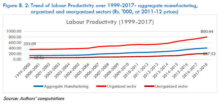 Average annual growth rates in labour productivity in the organised and unorganised segments and total manufacturing during 2000 to 2017 and the two sub-periods 2000-2007 and 2008-17 are depicted in Figure 8.3. It shows that the growth rate in labour productivity was higher in the unorganised segment than in the organised during 2000-2017 as well as in the two sub-periods. It is particularly interesting to observe a marked increase in the annual growth rate in labour productivity in the unorganised segment to 8.9 per cent in 2008-17 from 4 per cent in 2000-2007. As observed earlier unorganised manufacturing experienced a marked increase in the growth rate in real GVA and a fall in the growth rate of employment during 2008-17 as compared to 2000-2007. A marked increase in the growth rate in labour productivity is therefore expected. Interestingly, although the growth rate in real GVA in organised manufacturing decreased over the same period, there was a steeper decline in the employment growth rate, causing the growth in labour productivity to accelerate. Therefore, labour productivity in total manufacturing also experienced a faster growth in the period 2008-17. 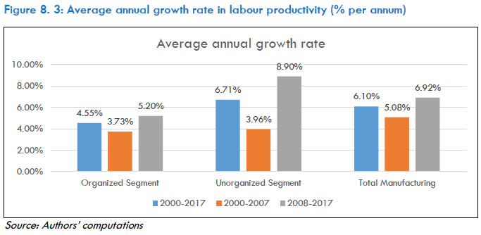 A further analysis of labour productivity for the 13 industries provides an understanding of the variation within the organised and unorganised segments. Table 8.6 presents this analysis of at three points of time, namely 1999-2000, 2008-09 and 2017-18 to capture the differences within segments and over time. It is evident that productivity in the unorganised sector is generally less than that in the organised sector. Between 1999 and 2017, the productivity of the organised sector increased and was about Rs 800,000 in 2017 as compared to only about Rs 200,000 for the unorganised sector. Over this period, although the absolute difference in labour productivity increased, the overall tendency for labour productivity in the two segments was of convergence and the ratio of labour productivity of the two narrowed from a multiple of 5.7 to a multiple of just 3.9. While the differences in labour productivity between the segments were small for some industries in 2017 for others, these differences were very substantial, e.g., in Food products, beverages and tobacco; Paper & paper products; Coke and petroleum products; and Machinery, n.e.c. The major reason for the variation could be differences in the enterprise-level production structures in the two segments. It is also evident from Table 8.6, that the industries with above average labour productivity in the organised segment in 1999-2000, are Coke and petroleum products, Chemicals and chemical products, Rubber and plastic products, Basic metals and metal products, Machinery, n.e.c. and Transport equipment. In 2017-18, five of these six industries except Chemicals and chemical products still enjoyed above average labour productivity. On comparison with the unorganised segment, there is variation in the gap between the labour productivity in the organised and unorganised segments. While the difference in labour productivity in 1999-2000 between the two segments is more than five times in Basic metals and metal products, it is just one and a half times for Electrical and optical equipment. In 2017-18, the difference in labour productivity between the two segments was 7.5 times for Food products, beverages and tobacco, but in the Transport equipment industry, and Wood and wood product industry, labour productivity in the unorganised segment was more than that in the organised segment. Over the period of 1999 to 2017, the convergence, visible at the aggregate level manufacturing sector, is also visible in eight out of 13 manufacturing industries. Three of these eight industries—Chemicals and chemical products, Rubber and plastic products, and Other manufacturing (Manufacturing, n.e.c.; recycling)—experienced convergence due to a rapid increase in labour productivity in the unorganised segment. In the other five industries, where divergence in the labour productivity is observed over time, four of them— Food products, beverages and tobacco, Paper and paper products, Coke and petroleum products, and Basic metals and metal products failed to achieve convergence between the organised and unorganised segments due to a large increase in labour productivity in the former. There is thus a tendency in a majority of the manufacturing industries, for convergence in labour productivity between the organised and the unorganised segments. We observe that this kind of catching up in labour productivity is possible only when the unorganised segment achieves a faster growth in labour productivity, which requires appropriate policy support. | There is a tendency for convergence in labour productivity between the organised and unorganised segments. This kind of catching up is possible only when the unorganised segment achieves a faster growth in labour productivity, which requires appropriate policy support. |
| Table 8.6: The level of labour productivity in organized and unorganized segments of Indian manufacturing in 1999, 2008 and 2017 | | (Rs.000) | | Industry | Organized segment | Unorganized segment | Organized and Unorganized segments combined | | 1999-2000 | 2008-2009 | 2017-2018 | 1999-2000 | 2008-2009 | 2017-2018 | 1999-2000 | 2008-2009 | 2017-2018 | | Food Products, Beverages and Tobacco | 190 | 424 | 710 | 46 | 68 | 95 | 73 | 142 | 224 | | Textiles, Textile Products, Leather and Footwear | 90 | 123 | 262 | 47 | 71 | 165 | 57 | 86 | 195 | | Wood and Products of wood | 68 | 40 | 86 | 37 | 37 | 98 | 38 | 38 | 97 | | Pulp, Paper, Paper products, Printing and Publishing | 188 | 282 | 479 | 86 | 118 | 123 | 121 | 186 | 262 | | Coke, Refined Petroleum Products and Nuclear fuel | 6134 | 8564 | 13058 | 144 | 127 | 55 | 4772 | 7051 | 9662 | | Chemicals and Chemical Products | 791 | 1005 | 1709 | 181 | 321 | 1175 | 516 | 805 | 1555 | | Rubber and Plastic Products | 396 | 430 | 696 | 118 | 210 | 688 | 270 | 338 | 693 | | Other Non-Metallic Mineral Products | 271 | 246 | 439 | 83 | 90 | 278 | 133 | 154 | 340 | | Basic Metals and Fabricated Metal Products | 625 | 825 | 1035 | 113 | 195 | 305 | 295 | 452 | 594 | | Machinery, nec. | 452 | 914 | 991 | 163 | 233 | 144 | 315 | 622 | 549 | | Electrical and Optical Equipment | 155 | 647 | 535 | 101 | 122 | 159 | 139 | 350 | 303 | | Transport Equipment | 457 | 606 | 1241 | 269 | 471 | 1764 | 404 | 577 | 1410 | | Manufacturing, nec; recycling | 117 | 45 | 149 | 42 | 42 | 127 | 53 | 43 | 132 | | All manufacturing | 353 | 482 | 800 | 62 | 87 | 208 | 136 | 213 | 409 | | Source: Authors’ computations | Figure 8.4 shows labour productivity of the organised and unorganised segments relative to the aggregate industry and reveals the heterogeneity that exists among the 13 industries of the manufacturing sector. In only one industry—Transport equipment— labour productivity in the unorganised segment was almost equal to that of the aggregate industry and had the least gap with labour productivity in the organised segment. A plausible explanation for this lies in the predominance of organised employment (more than 75 per cent) in the industry (Figure 8.5). However, barring the exception of Transport equipment, labour productivity in the organised segment of each industry is higher than that in its unorganised counterpart, with large gaps in some cases, e.g., Food products, beverages and tobacco, Electrical and optical equipment, Machinery, n.e.c., Basic metals and metal products, and Coke and petroleum products. It is clear from Figure 8.5 that in all these industries except Coke and petroleum products, the unorganised sector’s share in employment is quite high at 50 per cent or more, and this large unorganised segment has low labour productivity. The information in Figure 8.5 on the average shares of unorganised and organised segments in total employment at the industry level reveals that unorganised sector employment dominates in relatively traditional and low-tech industries—Food products, beverages and tobacco, Textiles and leather, Wood and wood products, Non-metallic mineral products, Basic metals and metal products, and Other manufacturing (Manufacturing, n.e.c. including recycling). The organised segment’s share in employment is relatively high in the more high-tech industries, e.g., in Transport equipment, Machinery, n.e.c., Rubber and plastic products, Chemicals and chemical products, and Coke and petroleum products.
8.7.2 Informality: Role in stagnant growth and sectoral decomposition In this section we try to understand how the persistence of employment in the unorganised sector acts as a dampener in the growth of overall labour productivity and whether any movement of labour from less-productive employment to more-productive employment could increase productivity and hence income level of workers. Figures 8.2 and 8.4 have revealed that the overall average manufacturing labour productivity and that of the 13 industries is lower in the unorganised sector despite its dominance in terms of employment in most industries. It would be interesting to know the extent to which the unorganised sector ‘drags’ down the labour productivity of the organised sector. We use equation 8.4 to find the ‘drag’ and present the results in Table 8.7. The table shows that the ‘drag’ is quite substantial over the period 2000-2017—it is more than 25 per cent of the aggregate productivity growth without informality. But the drag is slightly more in the second sub-period of 2008-17, when the aggregate labour productivity of the manufacturing sector increased by 2 percentage points. How do we explain the relatively bigger ‘drag’ in the period 2008-2017, pulling down the overall labour productivity in manufacturing? It seems that the explanation lies in the fact that while labour productivity of the unorganised sector during the two sub-periods grew faster and narrowed down the relative gap between the two segments but the absolute gap in the levels of labour productivity of the two segments has increased. | Table 8.7: Drag due to informality | | (Percent) | | | 2000-2007 | 2008-2017 | 2000-2017 | | Aggregate Labour Productivity growth | 5.33 | 7.21 | 6.37 | | Labour Productivity growth without informality | 7.62 | 9.77 | 8.82 | | Drag due to informality | -2.29 | -2.56 | -2.44 | | Source: Authors’ calculations | 8.7.3 Decomposition of aggregate labour productivity growth - the reallocation effect In this section, we analyse the contribution of structural change to aggregate labour productivity growth, in terms of workers’ movement across industries within the manufacturing sector—and further decompose it to the movement within and across the organised and unorganised segments, using the shift-share decomposition as expressed in equation 8.5. The results in Table 8.8 provide us the decomposition of manufacturing productivity growth between its two segments. While within industry changes measures change in productivity due to shift of labour within an industry over time, the structural change or static change denotes the change in productivity due to shift of labour from one industry to another. If the term is positive, it implies that labour is moving from less productive industry to more productive industry, and vice versa for a negative term. | Table 8.8: Decomposition of Productivity Growth in the Manufacturing Sector | | Period | Components due to | | | Within industry change | Structural Change | Aggregate labour productivity growth | | Organized | Unorganized | Total | Organized | Unorganized | Total | | | | (1) | (2) | (3) | (4) | (5) | (6) | (7) | | 2000-2007 | 3.43 | 1.38 | 4.81 | 0.89 | -0.37 | 0.52 | 5.33 | | 2008-2017 | 3.08 | 2.35 | 5.42 | 1.53 | 0.26 | 1.78 | 7.21 | | 2000-2017 | 3.23 | 1.92 | 5.15 | 1.24 | -0.02 | 1.22 | 6.37 | Source: Authors’ computations
Note: The totals may not sum up due to rounding off. | The table provides the magnitude of the reallocation effects – both within-industry productivity growth and static or structural change. The average aggregate productivity growth for the entire period of 2000-2017 is 6.4 per cent, 5.3 per cent in the first sub-period and 7.2 per cent in the second sub-period. In general, aggregate productivity growth is explained majorly by within-industry productivity growth (5.2 per cent out of 6.4 per cent for 2000-2017), and the remaining part (1.2 per cent) is attributed to between effect or structural change. The impact of overall reallocation has thus been throughout positive. The structural change effect was lower during the earlier period and increased substantially since 2008. Some of the reforms aimed at mitigating the adverse impact of the global financial crisis in 2008 might have incentivised these structural changes. Some positive outcomes of the development of global value chains and access to ICT might also have induced these structural changes. The contributions of organised and unorganised manufacturing to the within-industry productivity change and to structural change are shown in columns 1, 2, 4, and 5. The organised sector contributed more than 60 per cent to within-industry change during the period 2000-2017, although this share declined slightly in the second sub-period as compared with the first. The structural change in total manufacturing, although small, came from the organised sector—where workers moved from less productive industries to more productive industries. The contribution by the unorganised sectors on the other hand, is negative for the first sub-period, small and positive for the second sub-period, but negative for the overall period. This implies that labour either moved from more productive organised to less productive unorganised sectors, or from more productive unorganised to less productive unorganised sectors. The results are consistent with the results by Djidonou and McGregor (2020) for the period 1981-2011. | The structural change in total manufacturing, although small, came from the organised sector—where workers moved from less productive industries to more productive industries. The contribution by the unorganised sectors on the other hand, is negative for the overall period. | For a better understanding of the structural change in the manufacturing sector, we further decompose the structural change into within-industry and cross-industry effects. Within-industry structural change tells us about the movement between the organised and unorganised segment within each industry, whereas between-industry structural change gives us the movement of workers from organised and unorganised segments between different industries. The results obtained by using equation 8.6 are summarised in Table 8.9. It is evident that for the period 2000-2017, the total structural change is positive in both the sub-periods and can be attributed to both within-industry and across industry structural change. The contribution of within-industry structural change is positive in the first sub-period and this offsets the small negative change in the cross-industry sectoral change. However, the cross-industry structural change subsequently contributed substantially and has offset the negative within-industry structural change, resulting in the overall positive structural change. | Table 8.9: Decomposition of Manufacturing Productivity Growth by Organized / Unorganized Segments | | Period | Structural Change | | | Within industry | Cross-industry | Total Structural change | | Organized | Unorganized | Total | Organized | Unorganized | Total | | | 2000-2007 | 0.98 | -0.36 | 0.62 | -0.09 | -0.01 | -0.10 | 0.52 | | 2008-2017 | -0.13 | 0.13 | -0.01 | 1.66 | 0.13 | 1.79 | 1.78 | | 2000-2017 | 0.36 | -0.09 | 0.27 | 0.88 | 0.07 | 0.95 | 1.22 | | Source: Authors’ computations | Considering the decomposition of the effects between the organised and unorganised segments, the results show that the within-industry component is negative for the unorganised sector while the cross-industry structural change component is overall positive, albeit small—negative for first sub-period and positive for the second sub-period in this study. This means that one of the drivers of the relatively low structural change component has been the shift of employment within industries to less productive unorganised activities. While there has also been a movement towards more organised industries over time, this has not been large enough to offset the move to unorganised activities within industries. Conversely, the within and cross industries structural change components are positive for the organised segment for the entire period, but negative for within-industry structural change in the second sub-period and cross-industry change in the first sub-period 2000-2007—suggesting that overall, there has been structural change both within and across industries towards more productive organised activities. For the unorganised sector, the within-industry structural change is negative but the between-industry structural change is positive. It is thus obvious that while there has been some structural change within industries towards less productive unorganised activities, but when we consider cross industry movements, the workers are moving to more productive unorganised segments. | Considering the decomposition of the effects between the organised and unorganised segments, the results show that the within-industry component is negative for the unorganised sector while the cross-industry structural change component is overall positive, albeit small. | It is indeed heartening to note that workers are moving not only from less productive unorganised segments to more productive organised segments within an industry, but also across industries from less productive to more productive industries. This process may help in the overall formalisation of the manufacturing industry and in increasing its productivity. 8.8 Summary and Conclusion Manufacturing has always been considered an engine of growth in any economy and the experience of many developed and developing countries provides evidence of the key role it has played in economic development. However, there is also evidence of its limited role now in many developing and developed countries and a stage of ‘deindustrialisation’ might have set in these countries. Manufacturing sector in India, though it has played an important role—contributing 18 per cent to value added and 11.5 per cent to employment in 2017-18, but the shares have been quite stagnant, especially in employment. Because of the stagnation and its imminent role in economic development, policy makers have sought to focus on growth of this sector and the National Manufacturing Policy in 2011 and ‘Make in India’ in 2014 were designed with this objective. Manufacturing in India has a dualistic structure with both organised and unorganised sectors, but it has been dominated by the unorganised sector in terms of number of enterprises and employment, which had one-third share in GVA but two-third share in employment in 2017-18. These shares have persisted between the period of 1999 and 2017, with real GVA growing at 7.17 per cent in the unorganised sector and 7.26 per cent in the organised sector. The growth in the unorganised sector real GVA accelerated from 5.6 per cent during 2000-2007 to 8.5 per cent during 2008-17. On the other hand, the growth in employment during 2000-2017 in the unorganised sector has been much lower (0.46 per cent) than the organised sector (2.72 per cent). As a result, the organised sector accounted for 7 million new jobs of the total 10 million new jobs created in the manufacturing sector during the period. But all the 13 manufacturing industries show heterogeneity in the growth of GVA and employment, both in the organised and unorganised segments. Because of these differences in the 13 industries, there are significant differences in the level and growth in labour productivity across industries and across time. Labour productivity in the unorganised manufacturing segment has always been lower than that of the organised segment, though the relative difference has narrowed over time. Thus, the unorganised segment has exerted a downward pressure, a ‘drag’ on the labour productivity of the overall manufacturing sector as well as on its constituent 13 industries. The drag is more than 25 per cent of the aggregate productivity growth without informality, and it is slightly more in the second sub-period of 2008-17. The decomposition of the labour productivity growth shows a positive within-industry change and structural (or between-industry) change, thus pointing to the phenomenon of movement of workers from less productive to more productive industries as well as from less productive segments to more productive segments. This phenomenon along with an increase in employment in the organised sector augers well for the Indian economy in its quest for ‘formalisation’. | The unorganised segment has exerted a downward pressure, a ‘drag’ on the labour productivity of the overall manufacturing sector as well as on its constituent 13 industries. The drag is more than 25 per cent of the aggregate productivity growth without informality, and it is slightly more in the second sub-period of 2008-17. | A close analysis of the 13 industries may throw more policy options whereby focus could be laid more on those industries which could aid in accelerating the process of formalisation of Indian manufacturing, both from capital and labour points of view. It is important that impediments to the growth of the organised manufacturing sector are removed by taking appropriate policy initiatives to accelerate its growth. The firms in the unorganised sector must also be incentivised to grow and become competitive by removing obstacles through the provisioning of cheap finance, regular supply of electricity and other necessary inputs, access to new appropriate technology and markets. Some of these steps would go a long way in the holistic growth of the manufacturing sector in India. Annexure 8A: Construction of real GVA series for organized and unorganized segments of manufacturing industries Construction of real GVA series for organised and unorganised segments of the 13 KLEMS industries belonging to manufacturing involves several steps. These are described below: A. The computations start from the GVA series at current prices for the 13 KLEMS manufacturing industries (organised and unorganised segments combined) as given in India KLEMS database, 2019. These series are for the years 1980 to 2017 and are based on the NAS series with base 2011-12 and the corresponding back series. B. The GVA series at constant (2011-12) prices for different industries are also taken from India KLEMS database, 2019 and implicit deflators for GVA are computed for each of the 13 manufacturing industries. C. In the next step, GVA at current prices are constructed separately for the organised and unorganised segments of the 13 industries for the years 1980 to 2011 on the basis of national accounts data with base 2004-05 and the corresponding back series.146 Using GVA data for manufacturing industries available in the NAS series with base 2004-05 and the corresponding back series, GVA for the organised (registered) and unorganised (unregistered) segments of each of the 13 KLEMS manufacturing industries have been obtained for the years 1980 to 2011.147 These series are not directly use, but are used to split proportionately the series mentioned in (A) above into organised and unorganised components, for the years 1980 to 2011. D. Using ASI data, GVA at current prices is computed for each of the 13 manufacturing industries. Such series have been constructed for the years 1980 to 2017. ASI based GVA series is the organised segment for each of the 13 manufacturing industries. E. For each industry, the GVA series for the organised segment constructed in step-C is regressed on the series based on ASI (as in step-D) for the period 1999 to 2011 and then the estimated regression coefficient along with the ASI based series for the years 2012 to 2017 are used to extend the series for the organised segment obtained in step-C for the years 2012 to 2017. After computing GVA at current prices for the organised segment, that for the unorganised segment is obtained as residual (since total GVA is available for each industry each year from step A). F. However, in the case of one industry, namely ‘Coke, Refined Petroleum Products and Nuclear fuel’, the method described above encountered a problem. In the national accounts data with base 2011-12, GVA for manufacturing industries are split into two parts: corporate segment and household segment. The household segment is a part of the unorganised segment (as defined here). For Coke, Refined Petroleum Products and Nuclear fuel industry, the computed GVA for the unorganised segment was found to be less than that reported for the household segment in the national accounts data (with base 2011-12) for the year 2011-12 and for some later years.148 In this case, therefore, a slightly different method was applied. For 2011-12, the figure for household segment was treated as the estimate for the unorganised sector. For the years 2012-13 to 2017-18, an estimate of GVA for the unorganised segment was formed by taking the GVA figures for the household segment (available in NAS, base 2011-12) and multiplying it by a scale-up factor. The scale-up factor was formed by considering the GVA figures for household segment for the years 2007-08 to 2011-12 and the estimate for the unorganised segment made in step-E above (the latter divided by the former, after taking the annual average). Having obtained the estimates of GVA in the unorganised segment for the years 2011-12 to 2017-18, an estimate for the organised segment for these years was derived as residual (since the total GVA of the industry, organised and unorganised segments combined is known in step A). G. After obtaining GVA series at current prices for the organised and unorganised segments for each of the 13 manufacturing industries for the years 1980-81 to 2017-18, these were deflated to derive GVA at 2011-12 prices. The deflators used are those mentioned in step-B. Annexure 8B: Growth rate in real GVA series in organized and unorganized segments of manufacturing industries, 1981-2017 Industry-wise average annual growth rates in real GVA during 1981-2017 and the four sub-periods, 1981-93, 1994-2002, 2003-07 and 2008-17 are presented in Table 8B.1. Two interesting points emerge from it. First, in some of the industries, the average annual growth rate in real GVA during 1981-2017 was higher in the unorganised segment than in the organised segment, even though at the aggregate level, the growth rate in real GVA in the latter exceeds that in the former. This pattern is observed for Rubber and plastic products, Electrical and optical equipment and Transport equipment. Evidently, in these three industries, the relative share of the unorganised segment in real GVA of the industry had an upward trend. Second, even though at the aggregate level of unorganised manufacturing, real GVA grew faster during 2008-17 than in 2003-07, for several industries, the growth rate in GVA fell in 2008-17. Further, there was a marked increase in the GVA growth rate between the periods 2003-07 and 2008-17 in the unorganised segment of Rubber and plastic products and Transport equipment, and this tended to pull up the growth rate at the aggregate level of unorganised manufacturing in the latter period. | Table 8B.1: Average annual growth rate (percent) in real GVA, organized and unorganized manufacturing | | Industry | Organized manufacturing | Unorganized manufacturing | | 1981-2017 | 1981-1993 | 1994-2002 | 2003-2007 | 2008-2017 | 1981-2017 | 1981-1993 | 1994-2002 | 2003-2007 | 2008-2017 | | Food Products, Beverages and Tobacco | 8.35 | 11.24 | 5.66 | 12.35 | 5.02 | 4.60 | 4.95 | 6.83 | 6.49 | 1.19 | | Textiles, Textile Products, Leather and Footwear | 6.28 | 5.67 | 1.81 | 9.76 | 9.34 | 6.06 | 4.88 | 5.11 | 6.65 | 8.15 | | Wood and Products of wood | 3.29 | 0.39 | 0.79 | 6.70 | 7.62 | 0.39 | -2.85 | -2.90 | 2.25 | 6.64 | | Pulp, Paper, Paper products, Printing and Publishing | 5.30 | 5.66 | -1.61 | 17.73 | 4.85 | 5.35 | 6.76 | 5.28 | 8.57 | 1.97 | | Coke, Refined Petroleum Products and Nuclear fuel | 8.80 | 13.09 | 5.82 | 6.92 | 6.86 | -2.14 | -6.64 | 5.02 | -3.61 | -1.99 | | Chemicals and Chemical Products | 8.14 | 9.95 | 7.72 | 9.43 | 5.51 | 8.92 | 8.54 | 8.16 | 7.45 | 10.85 | | Rubber and Plastic Products | 8.57 | 11.16 | 5.80 | 1.77 | 11.11 | 10.23 | 9.59 | 11.56 | 5.35 | 12.31 | | Other Non-Metallic Mineral Products | 7.44 | 8.72 | 7.28 | 6.27 | 6.50 | 7.55 | 5.89 | 9.55 | 4.33 | 9.52 | | Basic Metals and Fabricated Metal Products | 5.50 | 4.66 | 7.38 | 9.43 | 2.94 | 5.80 | 2.63 | 7.07 | 9.91 | 6.73 | | Machinery, n.e.c. | 6.85 | 3.52 | 5.21 | 13.76 | 9.18 | 6.82 | 10.53 | 4.21 | 6.60 | 4.46 | | Electrical and Optical Equipment | 8.73 | 6.74 | 9.23 | 19.45 | 5.52 | 11.04 | 9.71 | 6.57 | 18.69 | 12.98 | | Transport Equipment | 7.58 | 5.19 | 8.80 | 10.08 | 8.33 | 11.25 | 6.14 | 10.16 | 7.61 | 20.69 | | Manufacturing, n.e.c; recycling | 9.79 | 13.64 | 5.82 | 4.09 | 11.23 | 7.04 | 4.79 | 3.76 | 11.10 | 10.90 | | All manufacturing | 7.24 | 7.59 | 6.33 | 9.89 | 6.29 | 5.95 | 3.63 | 5.81 | 7.22 | 8.45 | Note: Relative shares of different industries in aggregate manufacturing real GVA to show their relative importance and the relative share of the organized segment in 1999 are shown in Table 8.4.
Source: Authors’ computations | Annexure 8C: Growth in employment in organised and unorganised segments of manufacturing, 1981-2017 Growth rates in employment in organised and unorganised segments of Indian manufacturing in the periods 1981-1999 and 2000-2017 are shown in Table 8C.1 below. The growth rates in employment for aggregate manufacturing are also shown, which is based on the employment data contained in India KLEMS database 2019. It should be noted that the underlying methodology for the two sub-periods differ because of which the growth rates of employment in the organised and unorganised segments of manufacturing for the period 1981-1999 shown in the tables are not strictly comparable to those for the period 2000-2017. Yet, it would be safe to infer that the growth rate in employment in the organised segment was significantly higher in the period 2000-2017 than in the period 1981-1999, whereas the converse was true for the unorganised segment of manufacturing where a marked slowdown in employment growth took place in the later period. As regards total manufacturing, the growth rate in employment during 2000-2017 at about 1.1 per cent per annum was lower than that during 1981-1999 at about 2.0 percent per annum. This shows the same pattern as in the case of unorganized manufacturing. This is to be expected since the unorganised sector has a dominant share in employment in aggregate manufacturing. | Table 8C.1: Average annual growth in employment in the organized, unorganized and total manufacturing (1981-2017) | | Segment of manufacturing | 1981-82 to 1999-00* | 2000-01 to 2017-18** | | growth in employment (organized- Persons) | 0.23% | 2.72% | | growth in employment (Unorganized-Persons) | 2.54% | 0.46% | | growth in employment (Total) | 2.02% | 1.13% | Note: * the series of organized manufacturing employment from 1980-81 to 1999-00 is taken from ASI (total persons employed) and unorganized employment is the residual of total employment and organized employment.
** The series of organized and unorganized from 1999-00 to 2017-18 is obtained from EUS and PLFS, NSO.
Source: Authors’ computations | Chapter 9: Capital Intensity in Industries 9.1 Introduction Trends in the growth rates of capital stock and capital services have been discussed earlier in Chapter 5. This chapter is devoted to analysing the trends in capital intensity – capital to worker ratio and capital to output ratio. However, the focus is more on the trends in capital-labour ratio for two reasons: (1) this has implications for growth in labour productivity and TFP, and (2) this may have implications for employment generation. Capital deepening can augment labour by assisting workers and helping them improve their productivity. However, raising capital per worker may also lead to increasing substitution of workers with machines leading to adverse employment effects. Therefore, it is important for a country like India, with a significantly large number of young labour market entrants, to understand the trends in capital per worker. The Chapter is divided into five sections. Section 9.2 is devoted to discussing the trends in capital intensity and its growth rates. Both aggregate economy level trends and industry level trends are considered. Section 9.3 looks at the cross-industry relationship between growth in capital intensity and labour productivity. Section 9.4 deals with the role of movements in factor prices in inducing changes in capital intensity. The relationship between wage-rental ratio and capital intensity is studied. Finally, the findings and conclusions of the study are given in Section 9.5. All analyses in this Chapter are done for the period 1981 (1981-1982) to 2017 (2017-2018) and three sub-periods, 1981-1993, 1994-2002, and 2003-2017. In some sections of the Chapter, the last sub-period is split into two parts, 2003-2007 and 2008-2017. 9.2 Trends in capital intensity 9.2.1 Capital intensity in the aggregate economy and broad sectors Capital intensity, or capital deepening, measured as capital stock per worker, has been increasing quite rapidly in the aggregate economy, especially since 2008 (Figure 9.1). This has been true for both equipment capital stock (machinery and transport equipment assets) as well as non-equipment capital stock (construction). At the same time, the capital-output ratio, measured as capital stock per unit of real value-added, had been falling until the early 1990s and then started increasing. Despite some decline in the last two years since 2015, the general trend has been of growth. However, there are significant asset compositional differences here. While the capital to output ratio has been falling for non-equipment assets, it has been expanding for equipment, indicating the increasing mechanisation of production in the economy. 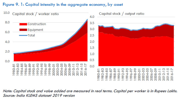
| Table 9.1: Capital deepening - ratios of capital stock to worker, and capital stock to output, by sector | | | Capital / worker ratio | Capital / output ratio | | 1981-1993 | 1994-2002 | 2003-2017 | 1981-1993 | 1994-2002 | 2003-2017 | | Agriculture & allied | 0.6 | 0.7 | 1.3 | 1.8 | 1.7 | 2.0 | | Mining & quarrying | 4.2 | 6.3 | 17.0 | 0.9 | 0.9 | 1.4 | | Manufacturing | 2.4 | 4.5 | 8.8 | 2.9 | 3.3 | 3.5 | | Utilities | 60.5 | 95.5 | 130.7 | 15.6 | 12.6 | 12.1 | | Construction | 0.6 | 0.9 | 2.3 | 0.4 | 0.6 | 1.4 | | Market services | 2.9 | 3.4 | 6.4 | 3.3 | 2.4 | 2.3 | | Non-market services | 9.5 | 11.0 | 18.7 | 6.0 | 5.1 | 5.8 | | Total economy | 2.0 | 2.8 | 5.6 | 3.2 | 3.0 | 3.2 | Note: Capital stock and value added are measured in real terms. Capital per worker is in Rupees Lakhs. Periods are respectively 1981-1993=1980-81 to 1993-94; 1994-2002=1994-95 to 2002-03; and 2003-2017=2003-04 to 2017-18
Source: India KLEMS dataset 2019 version | The aggregate picture presented above conceals several sectoral heterogeneities. For instance, the capital-worker ratio is relatively high in the utility sector and substantially low in agriculture and construction (Table 9.1). However, the capital intensity increased in all the seven broad sectors of the economy, including agriculture. For instance, it increased by about two times in agriculture, manufacturing, and services — both market and non-market, in the 2000s compared with the 1990s. The construction and mining sectors witnessed an even more rapid increase in the capital deepening rates. These trends suggest that the Indian economy is increasingly becoming capital intensive, and the rate of increase in capital per worker has been quite substantial over the last three decades. This is further established in Table 9.2, which depicts the average growth rates of capital intensity across the broad sectors of the economy. On average, the capital per worker ratio in th eaggregate economy increased faster in the 2000s, at an average rate of 6.7 per cent compared with 2-4 per cent in the 1980s and the 1990s. In the 1980s, mining, manufacturing and utility sectors were the main drivers of the economy’s capital deepening growth. In contrast, the increase in capital per worker ratio was very trivial in the services and agriculture sectors. In fact, the ratio contracted for the construction sector. During the 1990s, however, it was construction sector that saw the highest expansion in capital per worker while manufacturing sustained a growth rate of about 5 per cent. Other sectors where the growth rate of capital per worker improved are agriculture and non-market services, while the market services continued to see a weak growth rate. In the 2000s, most sectors improved their capital per worker-expansion rate from the 1990s, although the growth rate differed considerably across sectors. Construction saw a fall in the growth rate, although it still had one of the highest growth rates among the broad sectors. Agriculture, mining, and market services sectors have seen faster growth. On the contrary, the capital/output ratio, often considered an important determinant of labour productivity under Solow (1957)'s growth model (see McQuinn and Whelan, 2007), grew more moderately in most sectors across the entire period of study. In the 1980s, when the capital per worker ratio in the aggregate economy grew by 2.5 per cent, the capital-output ratio decelerated, suggesting that output grew faster than capital stock. Barring mining, manufacturing, and construction sectors, the other broad sectors had a negative growth rate. The situation changed in the 1990s, when mining, utility, and market services saw substantial contraction in the capital-output ratio, while the other sectors registered expansion, although at dismal rates in most cases. Construction was the sole sector that registered very high growth during this period. Overall, the economy did not see much expansion in the capital-output ratio. By the 2000s, however, almost all sectors, except manufacturing, had a positive capital-output ratio, indicating that capital outgrew output in most sectors, with the entire economy seeing just half a per cent average growth rate. The mining and construction sectors experienced the fastest expansion in their capital-output ratios. | Table 9.2: Growth rate of capital deepening (capital/worker, and capital/output), by sector | | | Capital / worker ratio | Capital / output ratio | | 1981-1993 | 1994-2002 | 2003-2017 | 1981-1993 | 1994-2002 | 2003-2017 | | Agriculture & allied | 1.5 | 2.5 | 6.0 | -0.3 | 1.0 | 0.9 | | Mining & quarrying | 6.3 | 1.7 | 10.8 | 3.9 | -2.9 | 5.2 | | Manufacturing | 5.4 | 5.0 | 6.3 | 1.4 | 1.3 | -0.6 | | Utilities | 4.7 | 2.6 | 2.8 | -0.9 | -1.9 | 0.1 | | Construction | -1.4 | 8.0 | 6.6 | 1.6 | 6.7 | 5.1 | | Market services | 0.2 | 1.5 | 6.6 | -2.1 | -3.4 | 0.7 | | Non-market services | 0.9 | 3.2 | 4.4 | -2.9 | 1.0 | 0.2 | | Total economy | 2.5 | 3.7 | 6.7 | -0.5 | 0.1 | 0.5 | Note: Note: Growth rates are simple averages of log changes.
Source: India KLEMS dataset 2019 version | These observations reinforce our earlier assertion that the Indian economy has been becoming increasingly capital intensive over the years. The amount of capital that workers work with has been going up substantially across all sectors. The capital-output ratio has been growing likewise, although at a slower pace, and as a more recent phenomenon. Overall, it appears that among the broad sectors of the economy, construction is the one that is increasingly becoming capital intensive, both in terms of capital per worker as well as capital per output. It may be noted that, interestingly, this is also a sector where productivity growth, both labour productivity and total factor productivity, has been very dismal compared with most other sectors (Erumban et al., 2019). This suggests that although the sector has become increasingly capital intensive, its ability to use those assets more productively may have been limited. The issue warrants attention but is beyond the scope of this paper. Although one could, prima facie, expect this phenomenon may be affected by the composition of capital stock in the sector, it may not be a valid argument until corroborated with adequate evidence. For instance, the share of equipment capital in the construction sector is not substantially lower than in other sectors, as we saw in the previous section. It is also essential to mention that the capital-output ratio is the reciprocal of capital productivity or output per unit of capital, just how we look at labour productivity. The fact that it is rising, although at a slower pace than capital per worker, is indicative of weakening productivity of capital across Indian industries. Indeed, the economy is becoming increasingly capital intensive, but the question remains whether those investments are productively used or efficiently allocated. The rise in the capital-output ratio will directly impact labour productivity, as workers are now left to work with more capital (machines, for instance). In the standard Cobb-Douglas production function, under strict assumptions of constant returns to scale, labour productivity is a direct function of total factor productivity and capital per worker. Following that rationale, the growth accounting approach, widely used in the KLEMS type of research, can decompose the contribution of capital per worker and TFP within the accounting framework, which is attempted in a later chapter (see, for e.g., Erumban and van Ark, 2018). 9.2.2 Capital intensity in the 27 KLEMS industries In the next step, an analysis of capital intensity trends is undertaken at the industry level. Table 9.3 reveals that most of the industries that were capital intensive in the 1980s remained thus in the 1990s and 2000s. In 16 out of these 27 KLEMS industries, i.e., 59 per cent of all industries, capital intensity was higher than the aggregate economy average in the 1980s. This increased to 18 industries in the subsequent sub-periods. This suggests that about 70 per cent of all industries sustained a higher-than-average capital per worker ratio since the 1990s. Moreover, all industries, except for transport services, have increased capital intensity over time. While some industries such as communication, public administration, chemicals, business services, transport equipment have seen a rapid increase in their capital per worker ratio over the period under study, other sectors saw a slower pace. The capital-output ratio also remains the highest in the petroleum and utility industries, followed by industries in non-market services sector. Although the capital-output ratio in sectors such as construction and agriculture improved faster in the 2000s, the pace of catch-up was not sufficient to reach closer to the very high capital/output ratio is in petroleum and non-market services. | Table 9.3: Capital intensity by industry, 1981-2017 | | Industry | Capital stock/worker | Capital stock/value added | | 1981-1993 | 1994-2002 | 2003-2017 | 1981-1993 | 1994-2002 | 2003-2017 | | Agriculture & allied | 0.6 | 0.7 | 1.3 | 1.8 | 1.7 | 2.0 | | Mining & quarrying | 4.1 | 6.3 | 17.0 | 0.9 | 0.9 | 1.4 | | Food pdts, beverages & tobacco | 1.8 | 3.0 | 6.4 | 3.9 | 4.1 | 4.4 | | Textiles & leather | 0.7 | 2.0 | 4.7 | 2.2 | 3.6 | 4.2 | | Wood & wood pdts. | 0.4 | 0.6 | 1.6 | 0.5 | 1.4 | 3.0 | | Pulp & paper pdts. | 17.6 | 21.8 | 20.3 | 14.8 | 17.1 | 10.4 | | Coke and petroleum pdts | 19.9 | 59.0 | 160.0 | 0.6 | 1.1 | 1.8 | | Chemicals & chemical pdts. | 8.4 | 12.7 | 22.6 | 3.7 | 2.6 | 2.4 | | Rubber & plastic pdts. | 4.0 | 10.0 | 15.4 | 2.9 | 4.2 | 4.3 | | Non-metallic mineral pdts. | 1.0 | 3.3 | 7.5 | 1.6 | 2.9 | 4.1 | | Basic metals & metal pdts. | 5.3 | 9.1 | 18.4 | 2.6 | 2.9 | 3.8 | | Machinery, n.e.c.. | 5.2 | 7.2 | 12.4 | 1.7 | 2.4 | 2.7 | | Electrical & optical eqpt. | 4.9 | 8.2 | 10.2 | 5.1 | 5.1 | 3.4 | | Transport eqpt. | 4.9 | 9.2 | 19.1 | 2.0 | 2.4 | 2.3 | | Other manufacturing | 1.1 | 2.2 | 3.4 | 5.4 | 5.8 | 5.7 | | Utilities | 59.4 | 95.5 | 130.7 | 15.7 | 12.6 | 12.1 | | Construction | 0.6 | 0.9 | 2.3 | 0.4 | 0.6 | 1.4 | | Trade | 0.3 | 0.4 | 1.7 | 0.5 | 0.5 | 0.9 | | Hotels & restaurants | 0.7 | 0.9 | 2.0 | 1.6 | 1.2 | 1.7 | | Transport & Storage | 9.8 | 8.7 | 9.1 | 10.7 | 7.5 | 4.7 | | Post & telecom | 8.8 | 12.3 | 24.5 | 7.0 | 5.7 | 3.2 | | Financial services | 6.5 | 11.1 | 12.1 | 1.5 | 1.4 | 1.1 | | Business services | 6.5 | 11.0 | 25.9 | 2.0 | 2.4 | 3.8 | | Public administration | 7.9 | 11.4 | 29.3 | 6.2 | 5.3 | 5.3 | | Education | 0.6 | 0.9 | 2.4 | 0.8 | 0.9 | 1.4 | | Health & social work | 0.8 | 1.6 | 4.5 | 1.1 | 1.3 | 2.0 | | Other services | 17.2 | 17.8 | 29.1 | 7.0 | 6.1 | 8.0 | | Total economy | 0.2 | 0.3 | 0.6 | 3.2 | 3.0 | 3.2 | Note: Capital stock and value added are measured in real terms. Capital per worker is in Rupees Lakhs
Source: India KLEMS dataset 2019 version | Considering the entire period, the average annual growth rate in capital intensity for the Indian economy was about 4.5 per cent during 1981-2017 (Table 9.4). The growth rate in capital intensity during this period was relatively much higher in the following industries: Mining & Quarrying; Textiles, Textile Products, Leather & Footwear; Coke, Refined Petroleum Products & Nuclear fuel; Non-Metallic Mineral Products; Trade; Education; and Health & Social Work. By contrast, the growth rate in capital intensity was relatively low (and even negative in one case) in the following industries: Pulp, Paper, Paper products, Printing & Publishing; Electrical & Optical Equipment; Transport & Storage; Financial Services; and Other Services. | Table 9.4: Growth rate in capital intensity (per cent per annum), by industry | | Industry | Share in capital stock (%), 1980-1984 | Avg capital intensity, 1980-1984 (Rs. Lakhs per person) | 1981-2017 | 1981-1993 | 1994-2002 | 2003-2017 | 2003-2007 | 2008-2017 | | Agriculture & allied | 22.0 | 0.5 | 3.6 | 1.5 | 2.5 | 6.0 | 4.4 | 6.8 | | Mining & quarrying | 1.0 | 3.0 | 7.0 | 6.3 | 1.7 | 10.8 | 11.1 | 10.7 | | Food pdts, beverages & tobacco | 2.0 | 1.5 | 5.4 | 3.5 | 5.5 | 7.0 | 7.6 | 6.8 | | Textiles & leather | 1.0 | 0.5 | 7.7 | 8.1 | 7.4 | 7.5 | 10.3 | 6.1 | | Wood & wood pdts. | 0.2 | 0.3 | 5.7 | 3.8 | 5.7 | 7.5 | 8.3 | 7.1 | | Pulp & paper pdts. | 1.8 | 12.4 | 1.8 | 6.8 | -2.8 | 0.3 | 1.2 | -0.2 | | Coke and petroleum pdts | 0.1 | 14.7 | 9.8 | 11.0 | 14.8 | 5.8 | 3.8 | 6.8 | | Chemicals & chemical pdts. | 1.8 | 8.4 | 3.7 | -0.3 | 5.7 | 5.9 | 5.7 | 6.0 | | Rubber & plastic pdts. | 0.1 | 2.9 | 6.4 | 7.8 | 7.5 | 4.6 | 5.0 | 4.4 | | Non-metallic mineral pdts. | 0.3 | 0.6 | 8.7 | 9.9 | 11.9 | 5.9 | 6.2 | 5.7 | | Basic metals & metal pdts. | 1.8 | 4.1 | 4.9 | 5.6 | 1.8 | 6.3 | 9.7 | 4.6 | | Machinery, n.e.c.. | 0.4 | 3.4 | 4.1 | 6.7 | 1.3 | 3.5 | 10.4 | 0.1 | | Electrical & optical eqpt. | 0.5 | 4.9 | 1.5 | 1.0 | 7.1 | -1.3 | 3.2 | -3.6 | | Transport eqpt. | 0.4 | 4.3 | 5.5 | 3.3 | 6.7 | 6.7 | 8.0 | 6.0 | | Other manufacturing | 0.4 | 1.1 | 4.5 | 2.5 | 7.0 | 4.7 | 4.8 | 4.7 | | Utilities | 8.2 | 48.0 | 3.4 | 4.7 | 2.6 | 2.8 | 2.0 | 3.3 | | Construction | 0.9 | 0.7 | 4.1 | -1.4 | 8.0 | 6.6 | 10.1 | 4.9 | | Trade | 1.1 | 0.3 | 7.0 | 1.2 | 2.7 | 14.6 | 9.8 | 17.0 | | Hotels & restaurants | 0.3 | 0.6 | 5.2 | 4.4 | -0.2 | 9.2 | 8.2 | 9.7 | | Transport & Storage | 12.8 | 10.2 | -0.3 | -1.0 | -3.2 | 2.0 | 2.5 | 1.8 | | Post & telecom | 0.6 | 7.0 | 5.3 | 3.9 | 0.5 | 9.3 | 1.2 | 13.3 | | Financial services | 1.3 | 6.3 | 1.6 | 0.2 | 6.8 | -0.4 | 0.2 | -0.6 | | Business services | 0.7 | 6.3 | 3.9 | 0.7 | 9.5 | 3.3 | 5.8 | 2.0 | | Public administration | 10.6 | 6.8 | 5.7 | 3.6 | 4.2 | 8.3 | 8.7 | 8.1 | | Education | 0.4 | 0.5 | 6.4 | 3.9 | 5.2 | 9.2 | 9.4 | 9.1 | | Health & social work | 0.2 | 0.6 | 7.1 | 6.4 | 5.6 | 8.6 | 11.7 | 7.1 | | Other services | 28.8 | 17.4 | 2.1 | -0.9 | 3.9 | 3.6 | 3.3 | 3.8 | | Total economy | 100.0 | 1.7 | 4.5 | 2.5 | 3.7 | 6.7 | 6.2 | 6.9 | Note: Average annual growth rates are shown in the table. Capital intensity is measured by the ratio of capital stock (at 2011-2012 prices) to number of persons employed. Average share in capital stock (at 2011-2012 prices) during 1980-1984 is shown in the second column to signify relative importance in terms of (initial period) value of capital stock.
Source: Authors’ computations using India KLEMS database, 2019. | Capital intensity grew faster during 1994-2002 than during 1981-1993 in 16 of the 27 industries. It grew at a faster pace during 2003-2007 than during 1994-2002 in 18 of the 27 industries. Thus, in two-thirds of the industries, the growth rate in capital intensity went up during 2003-2007, which was a period of high growth in the Indian economy. However, the growth rate in capital intensity in the more recent period 2008-2017 was higher than that during 2003-2007 in only eight out of the 27 industries—in fact, it declined in a majority of the industries. Yet, the growth rate in capital intensity at the aggregate economy level was higher during 2008-2017 than that during 2003-2007, which could in part be a consequence of compositional changes. Of course, the growth in capital intensity in some of those eight industries where it rose, was sharp enough to have pulled up the aggregate level. Consider, for instance, the sharp rise in annual growth in capital intensity between the two sub-periods from 1.2 per cent to 13.3 per cent in Post & Telecommunication and from 9.8 per cent to 17 per cent in Trade (see Table 9.3). Generally, the industries that had a relatively higher growth rate in capital intensity during 2003-2007 also had a relatively higher growth rate in capital intensity during 2008-2017. However, there are exceptions. In Machinery nec, the growth rate in capital intensity was high during 2003-2007, but not during 2008-2017. On the other hand, in Post & telecommunication, there was slow growth in capital intensity during 2003-2007, but a rapid growth in capital intensity during 2008-2017. Sources of aggregate economy capital intensity growth: Worker reallocation across industries vs. within industry increases in capital intensity In addition to analyzing the trends in capital deepening at industry, sectoral and macro levels, we also examine whether the observed growth rates in the macro level capital deepening are an outcome of within-industry capital deepening growth rates or inter-industry reallocation. To do so, we use a methodology, which is quite similar to the well-known shift-share analysis used for understanding worker reallocation in labour productivity, as employed in Goldar et al. (2017). The analysis has been done separately for the periods, 1981-1993, 1994-2002 and 2003-2017. Table 9.5 presents the results. | Table 9.5: Decomposition of aggregate economy level capital intensity growth rate (per cent per annum), by sub-periods | | Indicators | 1981-82 to 1993-94 | 1994-95 to 2002-03 | 2003-04 to 2017-18 | | Within-industry capital intensity growth rate | 1.57 (63 per cent) | 3.17 (85 per cent) | 5.02 (75 per cent) | | Static reallocation effect | 0.95 (38 per cent) | 0.54 (15 per cent) | 1.62 (24 per cent) | | Dynamic reallocation effect | -0.04 (-2 per cent) | 0.00 (0 per cent) | 0.02 (0 per cent) | | Aggregate capital intensity growth rate | 2.47 | 3.71 | 6.67 | Note: Computations made on the basis of decomposition analysis. Relative shares the three different effects are shown in parentheses.
Source: Authors’ computations using India KLEMS database, 2019. | The results of the decomposition analysis show that within-industry, increases in capital per worker generally sustained a relatively higher contribution to the economy-wide capital deepening growth rate. However, the static reallocation effect, which captures the effect of the movement of workers to industries with a relatively higher level of capital intensity, contributed about 38 per cent of the aggregate level capital intensity growth rate during 1981-1993. Evidently, inter-industry reallocation of labour (shifts of factors from labour intensive to capital intensive industries) contributed significantly to aggregate level capital intensity growth. The static reallocation effect was relatively smaller during 1994-2002, at 15 per cent, but it rose to 24 per cent during the period, 2003-2017. Notably, the aggregate level capital intensity growth rate increased by about three percentage points per annum between 1994-2002 and 2003-2017 and the same period saw the growth rate in capital intensity increase in 18 out of 27 industries (Table 9.4). The results of the analysis presented in Table 9.5 thus indicate that a sizeable part (about one-third) of the hike in the growth rate in capital intensity in this duration (between 1994-2002 and 2003-2017) is explained by the effect of the inter-industry reallocation of labour. However, the contribution of the within-industry effect to growth rate in capital intensity during 2003-2017 significantly exceeded that during 1994-2002 and was indeed a far more important factor explaining the hike. | About one-third of the increase in the growth rate in capital intensity between 1994-2002 and 2003-17 is explained by the effect of the inter-industry reallocation of labour. | 9.3 Growth in Capital Intensity, Labour Productivity and Real Wages Following the neo-classical production function logic, since raising capital per worker is expected to augment workers' ability to produce, capital intensity is expected to improve labour productivity in industries and the economy. We see a one-to-one correspondence between the two indicators in all the time periods considered (Figure 9.2).  Labour productivity and capital intensity growth rates were quite similar in the 1990s and 2000s (1994-2002 and 2003-2007), whereas labour productivity grew faster in the 1981-1993 period and slower in the post-crisis period, compared to capital deepening. Both indicators grew much faster in the 2003-2017 period compared to 1981-2002 period. It should be pointed out here that the growth rate in real (product) wage rate149 at the aggregate economy level was also higher during 2003-2017 as compared with 1981-2002, thus showing the same pattern as capital intensity and labour productivity. The average annual growth rates in real (product) wage rate are found to be 2.3 per cent for 1981-1993, 3.2 per cent for 1994-2002 and relatively much higher at 6.2 per cent for 2003-2017. This reflects a positive association over time (specifically over the sub-periods we studied) among the growth rates in capital intensity, labour productivity and real wages at the aggregate economy level. | When the changes in growth rates in capital intensity and labour productivity between 1994-2002, and 2003-2017 are considered at the industry level, a clear, strong positive association is not found | Interestingly, when the changes in the growth rates in capital intensity and labour productivity between the sub-periods 1994-2002, and 2003-2017 are considered at the industry level, a clear, strong positive association is not found. This can be seen in Figure 9.3. In 14 industries, capital intensity growth was higher during 2003-2017 than during 1994-2002 and the same holds for labour productivity. In 4 industries, there was a fall in the growth rate in capital intensity and this was accompanied by a fall in the growth rate in labour productivity. But, in the remaining 9 industries, a hike in the growth rate in capital intensity was not accompanied by an increase in the growth rate in labour productivity (examples: Basic Metals & Fabricated Metal Products; Hotel & Restaurants; and Post & Telecommunication) or a fall in the growth rate in capital intensity in the period was accompanied by a hike in the growth rate in labour productivity (examples: Non-metallic Mineral Products; and Rubber & Plastic Products). The explanation for these divergences lies in the growth rates in TFP achieved. The fact that in Basic Metals & Fabricated Metal Products; Hotel & Restaurants; and Post & Telecommunication, a hike in capital intensity growth rate during 2003-2017 did not translate into a hike in the growth rate in labour productivity is explained by a fall in the growth rate in TFP (value-added based). Similarly, the fact that in Non-metallic Mineral Products; and Rubber & Plastic Products, a fall in the growth rate in capital intensity during 2003-2017 did not result in a fall in the growth rate in labour productivity can be traced to an increase in the growth rate in TFP (value-added based). | Considering the movements in the growth rates in capital intensity and real (product) wage rate between sub-periods and considering also the industry-wise pattern revealed by Figure 9.4, it seems reasonable to argue that a relatively faster growth rate in real (product) wage rate during 2003-2017 was responsible, at least to some extent, for the hike that took place in the growth rate in capital intensity (and hence the growth rate in labour productivity) during 2003-2017. | Along with the changes in the growth rates in capital intensity and labour productivity, Figure 9.3 also shows the change in the growth rate in real (product) wage rate150 at the industry level between the periods 1994-2002 and 2003-2017. The changes in the growth rates in real wage rate are highly correlated with those in labour productivity, with a correlation coefficient of 0.86. The correlation coefficient for changes in the growth rates in capital intensity and real (product) wage rate is found to be 0.24. While Figure 9.3 indicates some similarity between the changes in the growth rates in capital intensity and in real (product) wage rate, there are differences as well. As mentioned above, at the aggregate economy level, the growth rate in real (product) wage rate was about 3.2 per cent per annum during 1994-2002 which went up to about 6.2 per cent during 2003-2017. Considering the movements in the growth rates in capital intensity and real (product) wage rate between sub-periods and considering also the industry-wise pattern revealed by Figure 9.3, it seems reasonable to argue that a relatively faster growth rate in real (product) wage rate during 2003-2017 was responsible, at least to some extent, for the hike that took place in the growth rate in capital intensity (and hence the growth rate in labour productivity) during 2003-2017. This receives further attention in in the analysis carried out in the next section. To probe this issue further, a regression analysis was undertaken using aggregate economy level time series data for the years 1980-1981 to 2017-2018. The model specification and regression results are reported in the next section. The results point towards a positive effect of the wage-rental ratio on capital intensity. It may be inferred accordingly that an increase in real wages and/or a lowering of cost of capital will tend to raise capital intensity. This is logical because if the price of one input (labour) goes up relative to another input (capital), then the former input will be substituted by producers by the latter input to reduce cost of production, and thus cause the ratio of capital to labour to rise. Thus, the results of the econometric analysis indicate that the finding of a marked increase in the growth rate in real wages during 2003-2017 as compared to 1981-2002 fits well with (and may be treated as a major explanation for) the finding of an accelerated growth in capital intensity in the Indian economy during 2003-2017. 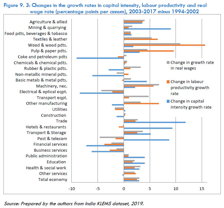 9.4 Wage-rental ratio and capital intensity of the Indian economy: Econometric Analysis 9.4.1 Relative prices of capital As the India KLEMS capital service estimation involves imputing the rental price or user cost of capital, it is also possible to evaluate the trends in the wage rental ratio or the relative price of capital. The importance of the relative price of capital for economic growth is well established in the literature (e.g., Jones, 1994). One would expect a negative relationship between the relative price of capital, especially equipment capital that drives positive composition effect, and economic growth. Table 9.6 provides the indices of wage rental ratio,151 measured by dividing the average wage rate (wage per worker) and the average rental price of the aggregate capital stock. | Table 9.6: Indices of wage-rental ratios, by broad sectors | | | 1981-1993 = 100 | Total economy = 100 | | 1981-1993 | 1994-2002 | 2003-2017 | 1981-1993 | 1994-2002 | 2003-2017 | | Agriculture & allied | 100.0 | 136.6 | 230.8 | 74.8 | 62.9 | 48.2 | | Mining & quarrying | 100.0 | 186.1 | 509.9 | 134.9 | 154.5 | 192.0 | | Manufacturing | 100.0 | 156.6 | 333.6 | 79.5 | 76.6 | 74.0 | | Utilities | 100.0 | 159.3 | 302.0 | 494.1 | 484.5 | 416.7 | | Construction | 100.0 | 154.7 | 245.5 | 196.8 | 187.4 | 134.9 | | Market services | 100.0 | 186.5 | 432.2 | 112.2 | 128.8 | 135.4 | | Non-market services | 100.0 | 141.2 | 247.7 | 420.5 | 365.6 | 290.9 | | Total economy | 100.0 | 162.4 | 358.1 | 100.0 | 100.0 | 100.0 | | Source: India KLEMS dataset 2019 version | The wage-rental ratio has increased over years, across the board. Clearly, wages have increased much faster than the rental prices of capital. The rate of increase in the market economy has been quite high in mining, market services, manufacturing, and utilities. Mining, utilities, and market services were also among those sectors with relatively higher wage/rental ratios compared with the aggregate economy (see the right panel of Table 9.6). On the other hand, the wage-rental ratio for manufacturing was only 3/4th that of the entire economy. The aggregate economy-wide wage-rental ratios might have been heavily driven by the services sector, including the very high wage/rental ratio in the non-market services. In fact, all the broad sectors of the economy, except agriculture and manufacturing, had a higher-than-average wage rental ratio. The rising trend in wage-rental ratio across the board clearly indicates that capital has been becoming relatively cheaper for Indian industries over time. It would be interesting to research the precise relationship between relative prices of capital by differentiating between the equipment and non-equipment capital and economic growth using detailed sectoral data. 9.4.2 Effect of Wage-rental ratio on and capital intensity – Aggregate Economy To assess the impact of changes in wage-rental ratio on capital intensity of the Indian economy at the aggregate level, an econometric model has been estimated. A production function underlies the model. It is assumed that there exists an aggregate level production function (or to be more specific, a value-added function) for the Indian economy. The form of the function is assumed to be CES (constant elasticity of substitution). Based on the CES value-added function, with additional assumption of cost minimisation, the following regression equation may be derived: In this equation, K denotes capital input, L denotes labour input and (w/r) is the wage rental ratio. The subscript t denotes time (year), and u is the random error term. Under the assumption of a CES production function and cost minimisation behaviour on the part of the producers, the coefficient of the wage-rental ratio in the above equation is expected to be positive, since an increase in wage rate, with the rental of capital remaining the same, should cause substitution of labour by capital and thus raise capital-labour ratio. The above equation has been estimated from time series data for aggregate Indian economy for the years 1980-81 to 2017-18, making use of the India KLEMS dataset, 2019. K is measured by capital stock and L is measured by the number of persons employed.152 Total wage bill is computed for each industry (by multiplying wage share in value added by gross value added at current prices) and then added together to derive the wage bill at the aggregate level. This is divided by L to compute w. Total wage bill is subtracted from aggregate gross value added and then divided by K to compute r. Then, the ratio of w to r is taken. Figure 9.4 gives a graphic presentation of the data on capital intensity and wage rental ratio (an index is formed and shown). A strong positive correlation between the two series is clearly observed from the figure. 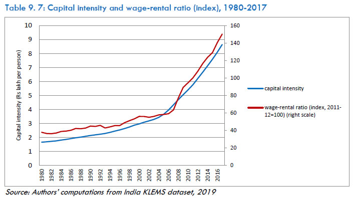 In equation 9.1 above, the coefficient of time captures the effect of non-neutral technical change. In actual application to time series data at the aggregate economy level, this coefficient will pick up not only the effect of non-neutral technical change but also the influence of some of the other changes taking place in the economy. It is particularly important to recognise that structural changes taking place in the economy may impact capital intensity and this may get reflected in the coefficient of the time variable. To incorporate this aspect into the analysis, a slightly modified model has been estimated as well in which the share of the agriculture and allied sector in aggregate GVA has been introduced in the model as an additional explanatory variable. Let GVAA denote real GVA in the agriculture and allied sector, and GVAtotal denote aggregate real GVA of the economy, then, the modified model may be written as:  The estimates of equations 9.1 and 9.2 given above are presented in Table 9.7. Two estimates each are presented for the two equations—one based on the ordinary least squares (OLS) method, the other based on Prais-Winsten regression. Since the DW statistic for the regression estimate based on OLS clearly indicates the presence of autocorrelation, which is likely to affect the parameter estimates, the Prais-Winsten regression has been applied. The regression results presented in Table 9.7 clearly indicate a positive effect of wage-rental ratio on capital intensity (as expected), notwithstanding the fact that the results are affected by autocorrelation (as signified by the DW statistic). There is some indication that a structural shift from agriculture sector to other sectors of the economy has had a positive effect on the capital intensity of the economy (i.e., it tends to raise capital intensity). It needs to be recognised that the econometric results in respect of the variable representing agriculture sector share in aggregate GVA are weak and the inference is based on finding of a negative coefficient. Since, among various sectors of the economy, the agriculture sector is relatively more labour intensive, a structural shift away from agriculture is obviously likely to reduce labour intensity and raise capital intensity. The regression results are in line with this expectation. | Table 9.8: Model explaining capital intensity, Indian economy, Regression Results | | Dependent variable: ln (capital-labour ratio) Period: 1980-81 to 2017-18 (n = 38) | | Explanatory variable | Regression-1
[OLS] | Regression-2
[Prais-Winsten] | Regression-3
[OLS] | Regression-4
[Prais-Winsten] | | ln (wage-rental ratio) | 0.686***
(19.32) | 0.303***
(5.30) | 0.581***
(14.56) | 0.298***
(5.07) | | ln (share of agriculture and allied sector in aggregate real GVA) | | | -0.602***
(-3.96) | -0.038
(-0.44) | | Time (year) | 0.0195***
(14.38) | 0.0334***
(10.30) | 0.0064*
(1.84) | 0.0325***
(8.48) | | Constant | -38.1 | -64.31 | -12.28 | -62.58 | | R-squared | 0.996 | 0.920 | 0.997 | 0.921 | | DW statistic | 0.553 | 0.854 | 1.17 | 0.874 | Note: t-ratios in parentheses. *, *** statistically significant at the one and ten percent level, respectively
Source: Authors’ computations based on India KLEMS dataset, 2019 | 9.4.3 Impact of real wage on capital intensity – estimate for manufacturing based on a panel data model In Section 9.4.2, an analysis of the impact of real wages on capital intensity was undertaken using aggregate economy level time series data. In this section, a supplementary analysis is undertaken. This is confined to manufacturing. Panel data on 13 manufacturing industries for the years 1980 to 2017 have been used to estimate an econometric model to assess the impact of real wages on capital intensity. The basic equation, derived from a CES production function, may written as):  In this equation, i is subscript for industry, and t is the subscript for time (year); K denotes capital, L labour,153 w wage rate, and r or pk rental of capital input. Since the rental of capital input pk may be written as pI(π+δ) where pI is the price (index) of investment (capital) goods (varies over time, but may be taken to be same for different industries), π is the rate of interest applicable to the industry (varying over time) and δ is the rate of depreciation for the industry (it is based on the composition of capital assets, and it may be treated as time invariant), the above equation may be written as : Which may be transformed to (allowing for some approximation):  The term w* denotes real wage rate (i.e., w/pQ), pl is the price of Investment (capital) goods, and pQ is the price of output. It is assumed that the terms π and δ would vary across industries and time, and these variations are largely picked up by the industry dummies (ɸ’i) and year dummies (λ’t) in the model, which will also capture other industry specific effects as well as time specific effects. The above equation has been estimated by applying the fixed effects model – for 1980-2017, and sub-periods. The results are shown in Table 9.8. A significant positive effect of real wages on capital intensity is found, implying thereby that hikes in real wages lead to increase in capital intensity. The coefficient of real wages which could be treated as the elasticity of substitution is found to be lower during 1980-1993 than that for 1994-2017. It appears that the labour-capital elasticity of substitution went up in the post-reform period. | Table 9.9: Model Explaining Capital Intensity – Industry Level Analysis, Fixed Effects Model | | Dependent variable: ln (capital-labour ratio) | | Explanatory variables | Period: 1980-2017 | Period: 1980-1993 | Period: 1994-2002 | Period: 2003-2017 | | ln(real wages) | 1.04 (14.91)# | 0.42(2.83)# | 0.84(7.03)# | 0.84(11.69)# | | ln(real price of investment goods) | -0.97 (-13.64)# | -0.61(-3.82)# | -1.01(-6.21)# | -0.77(-9.36)# | | Constant | 1.77 | 2.52 | 2.94 | 2.98 | | Number of observations | 494 | 182 | 117 | 195 | | R-squared | 0.83 | 0.58 | 0.75 | 0.86 | | F value and prob. | 86.2 (0.000) | 23.5 (0.000) | 27.5(0.000) | 52.4(0.000) | Source and note: Authors’ computations. Year dummy variables are included. t-values in parentheses.
# statistically significant at the one percent level. | From a test of serial correlation carried out on the model data, it is found that there is a clear indication of serial correlation. The F-value for the Wooldridge test of autocorrelation in panel data is found to 80.5 at (1, 12) degrees of freedom; this is statically significant. To address this model estimation issue, the Dynamic OLS method (DOLS) has been applied. The results remain by and large the same – only the coefficient of the capital rental price goes down somewhat. The estimates for the period 1980-2017 are shown in Table 9.9. | Table 9.10: Model Explaining Capital Intensity – Industry Level Analysis, DOLS, 1980-2017 | | Dependent variable: ln(capital-labour ratio) | | Explanatory variables | Regression-1 | Regression-2 | | ln(real wages) | 1.22 (8.84)# | 1.20(10.08)# | | ln(real price of investment goods) | -0.52(-3.28)# | -0.47(-3.19)# | | Trend | - | 0.006(0.99) | | Constant | - | - | | Number of observations | 442 | 442 | | R-squared | 0.91 | 0.97 | | Wald chi-square and prob. | 325.1 (0.000) | 243.3 (0.000) | Source and note: Authors’ computations. t-values in parentheses.
# statistically significant at the one percent level. | The results reported in Tables 9.8 and 9.9 clearly point to a significant positive effect of real wages on capital intensity – hikes in real wages tend to push up capital intensity. This is consistent with the findings of analysis presented in Section 9.4.2 of the chapter. In the econometric model estimates presented in Tables 9.7, 9.8 and 9.9, we implicitly assume that the factor prices are exogenous and the enterprises are deciding on the amount of labour and capital inputs to be used based on the factor prices. This assumption may be justified in firm-level or plant-level analysis since they are price takers. However, in industry or economy level analysis, as in our case, the possibility of a reverse causality cannot be dismissed because changes in factor supply and use may impact factor prices. Therefore, equation (9.6) has been also estimated by applying the Generalized Method of Moments (GMM) estimator. The results are presented in Table 9.10. For making these estimates, the time dummies have been dropped. The results show a significant positive effect of real wages and a significant negative effect of real price of investment goods on capital intensity. Thus, the main finding of the econometric analysis remains unaffected even if an estimation method is employed that can take care of the issue of reverse causality, at least to some extent. | Table 9.11: Model Explaining Capital Intensity – Industry Level Analysis, GMM, 1980-2017 | | Dependent variable: ln(capital-labour ratio) | | Explanatory variables | Regression | | ln(capital-labour ratio) (t-1) | 1.142 (5.66)# | | ln(capital-labour ratio) (t-2) | -0.269(-1.61) | | ln(real wages) | 0.158 (2.46)** | | ln(real price of investment goods) | -0.251(-2.38)** | | Constant | 0.299(1.29) | | Number of observations | 468 | | Wald chi-square and prob. | 325.1 (0.000) | | AR(1), prob. | 0.11 | | AR(2), prob. | 0.69 | | Sargan test, Chi-squared, and prob. | 8.1 (1.0) | Source and note: Authors’ computations. t-values in parentheses.
**, # statistically significant at the five and one percent level, respectively. | 9.5 Conclusion This chapter dealt with trends in capital intensity of Indian industries. The Chapter observes that the Indian economy is becoming increasingly capital intensive. Capital stock per worker has increased substantially over years and across industries. So has the capital-output ratio, although it is more of a recent phenomenon, and the rate of expansion is much lower. Among the broad sectors of the economy, the construction sector is the one that is increasingly becoming capital intensive. However, this sector seems to fail in translating its disproportionate use of capital into productivity, which is a subject that needs further scrutiny. Much policy attention has been given to improve India's manufacturing sector throughout India's history of economic policies. Interestingly, the manufacturing sector, which has a capital-output ratio closer to the aggregate economy average, maintains one of the weakest capital-output growth rates among the broad sectors of the economy. Simultaneously, it has a high capital per worker ratio and is one of the sectors with high growth in capital per worker. However, the wage-rental ratio in the sector is relatively lower. In fact, it is the second lowest after agriculture among the broad sectors of the economy. The rising capital per worker, stagnant capital-output ratio, yet with a relatively lower wage-rental ratio compared with other sectors, makes jobless growth in Indian manufacturing a continuing question (see Bhalotra, 1998, Tejani, 2015 and Verma, 2012, among others, for discussion on jobless growth in India). Because, if the relative price of workers in the manufacturing sector is still lower than many other sectors of the economy, the incentive for increased capital deepening lies not necessarily in labour cost, but in other considerations, which might include rigidities in the labour market, technology, or other policy constraints. Further research could explore this. Further research on the precise relationship between relative prices of capital and economic growth using the detailed sectoral data and by differentiating between the equipment and non-equipment capital would also provide useful insights. Another important observation is that the Indian economy is becoming increasingly capital intensive. Capital stock per worker has increased substantially across the board. So has the capital-output ratio, although it is more of a recent phenomenon, and the rate of expansion is much lower. Among the broad sectors of the economy, the construction sector is the one that is increasingly becoming capital intensive. However, this sector seems to fail in translating its disproportionate use of capital into productivity, which is a subject that needs further scrutiny. The faster increase in the capital per worker in the economy also comes along with a rapid rise in the wage-rental ratio. The average wage per worker in India has increased much faster than the rental prices of capital, suggesting that capital is becoming relatively cheaper. Although there are variations in the change in the wage-rental ratio, the rapid increase is a reality across all sectors. Perhaps, the faster rise in the capital per worker across the board may be explained by the falling relative price of capital. Future research may consider exploring what drives capital accumulation in the Indian economy. While we provide a general overview of the relative price of capital (compared to labour), several factors might be driving the decline in capital prices. For instance, the rapid declines in ICT prices have contributed to the increased investment in ICT assets globally since the 1990s. In general, innovation in the capital-producing sector - globally or locally - may have a direct or indirect effect on capital accumulation, as they can affect the relative price of equipment capital, indicating spillover effects from R&D spending on capital accumulation As regards inter-temporal variation, the analysis presented in the chapter revealed that the growth rate in capital intensity in the Indian economy was much higher during 2003-2017 (over 6.5 per cent per year) than that during 1980-1993 and 1994-2002. This accelerated growth obviously had adverse implications for job creation. It is particularly important to note that although annual employment growth between 1999 and 2011 was positive at about 1.4 per cent, it declined and became negative between 2011 and 2017 at about (-)0.2 per cent. As the number of new entrants into the labour force increases in the coming years, appropriate policy action is needed to contain the growth in capital intensity of production, particularly in manufacturing, and thereby help create more jobs. | Initial examination of trends in capital intensity, labour productivity and real wage rate followed by a more sophisticated econometric analysis of the impact of wage rental ratio on capital intensity indicated that the explanation for the marked rise in the growth rate in capital intensity in the period 2003-17 probably lies largely in an increase in the growth rate in real wages. | Initial examination of trends in capital intensity, labour productivity and real (product) wage rate followed by a more sophisticated econometric analysis of the impact of wage rental ratio on capital intensity indicated that the explanation for the marked rise in the growth rate in capital intensity in the period 2003-2017 probably lies largely in an increase in the growth rate in real wages. One possible area of policy action that might help in moderating the rise in capital intensity lies in containment of growth in prices of wage goods (e.g., increases in food prices) which will arguably help in containing the growth in real (product) wages to the extent possible. A second, and more promising, area of policy action lies in promotion of micro, small and medium enterprises (MSMEs). The contribution that such enterprises may make towards job creation is well recognised. However, in a global economic situation marked by recessionary conditions and intense competition in global markets, it is important to ask how the MSME sector in India may be given a major boost, particularly how to help them become capable of competing in global value chains. This obviously calls for appropriate policy for further promotion of MSMEs with support for improving their competitiveness. It needs to be recognized in this context that although there are a number of schemes for the promotion of MSMEs in India (and other supporting policy measures), such enterprises face several serious challenges constraining their performance and growth, the two important ones among them being related to (a) availability of credit and risk capital, and (b) adoption of superior technology and achievement of high product quality standards. Needless to say, adequate access to credit, adoption of superior technology, advancement in product quality, step-up in infrastructure facilities, and other such improvements will enable India’s MSMEs to get much better integrated into global value chains which will in turn contribute to the growth of the sector. These improvements will also help in building stronger linkages between the large industrial enterprises in India and the MSMEs, again favourable to MSME sector growth. An issue that needs to be highlighted here is that the MSME sector is dominated by micro enterprises, both in number and employment share, which very often remain in the same size class and do not grow in size over time into a small-scale enterprise or a medium-scale enterprise. The preponderance of enterprises that are very small in size and thus not in a position to take advantage of advanced technology with concomitant improvements in product quality is a serious handicap adversely impacting the progress of the MSME sector. To address this issue, an enabling business environment needs to be created for the MSMEs which will facilitate and provide ample incentives to micro enterprises to grow bigger in size and thus reap the associated gains in competitiveness. Attention may be drawn here to the sustainable development goals, particularly SDG-9. The goal is to “build resilient infrastructure, promote inclusive and sustainable industrialisation, and foster innovation.” Two components that need particular attention are: 9.2: Promote inclusive and sustainable industrialisation and, by 2030, significantly raise industry’s share of employment and gross domestic product, in line with national circumstances”, and 9.3: Increase the access of small-scale industrial and other enterprises, in particular in developing countries, to financial services, including affordable credit, and their integration into value chains and markets.” To raise industry’s share in employment and GDP requires policies that help in changing the structure of the India’s economy from a service-driven one to a manufacturing-driven one. The emphasis placed by the government on manufacturing sector growth and creation of manufacturing sector jobs is clearly reflected in the National Manufacturing Policy (NMP) of 2011 and the Make-in-India (MII) programme launched in 2014. The NMP had, in 2011, set a target of raising the then prevailing 15 per cent share of manufacturing in aggregate GDP (gross domestic product) to about 25 per cent in about 10 years, and creating 100 million new jobs in that process. To support the NMP and MII, significant advancements have been made with regard to the ease of doing business and efforts are underway for making further progress in this regard, apart from other initiatives for improving infrastructure etc. But, even if it becomes possible to raise the share of manufacturing in GDP in the years to come, this may not by itself raise the share of industry in employment unless there is a major boost to MSMEs. Towards this end, as stated above, there are several important policy questions that need careful consideration— such as, how the capacities of such enterprises could be built for better credit, technology and market linkages—particularly, for them to get integrated into global value chains, which now constitute a significant aspect of global trade and investment. Chapter 10: Energy Intensity in Manufacturing Industries This chapter deals with energy intensity of the Indian industries. The analysis is confined to manufacturing.154 An analysis of trends in energy intensity is presented in Section 10.1, which is followed by an econometric analysis of the determinants of energy use and energy intensity in Section 10.2. A distinguishing feature of the analysis is that energy intensity is computed by taking a physical measure of energy (discussed further later). Section 10.1 has three sub-sections— 10.1.1 deals with trends in energy intensity at the aggregate manufacturing level, covering both organised and unorganised segments. Section 10.1.2 examines trends in energy intensity in organized manufacturing, both at the aggregate level and for the 13 KLEMS manufacturing industries. Section 10.1.3 briefly discusses the impact of changes in real energy price on energy demand/consumption in organised manufacturing, drawing on the results of an econometric analysis of determinants of energy use and energy intensity in organised manufacturing presented later in Section 10.2 (additional econometric analysis is presented in Annexure 10C). The final section of the chapter, Section 10.5, summarises the findings and concludes. An attempt is made to draw some policy implications of the empirical findings. 10.1 Energy intensity A study of trends in energy intensity in the Indian economy assumes significance for the following reasons: (a) a lowering of energy intensity inasmuch as it is attained through greater efficiency in energy use contributes to competitiveness of domestic industries, and (b) how energy intensity of the Indian economy will change over time in the coming years, conceivably as indicated by the past trend, has important implications for India being able to meet her commitments on the containment of emissions intensity made under the United Nations Framework Convention on Climate Change (UNFCCC).155 Additionally, reduced dependence on energy input in the production activity in energy-intensive industries would relax supply side constraints arising from inadequacies of (or disruptions in) energy supply that might be adversely impacting their growth process. Among the various broad sectors of the Indian economy, manufacturing is the biggest user of energy. In recent years, the share of manufacturing in energy consumption in the Indian economy has been a little more than half (after disregarding energy use by households and non-energy use of natural gas and some petroleum products). A distinguishing feature of this analysis is that energy intensity is computed by taking a physical measure of energy. Among the studies on energy intensity in Indian manufacturing (Reddy and Ray, 2010; Ray, 2011; Goldar, 2011, 2012, 2013; Sahu and Narayanan, 2010, 2011; Soni et al. 2017; among others), some have used a physical measure of energy to compute energy intensity (taking the ratio of energy consumed in physical units to deflated value of output) and some others have used a value measure (energy intensity is obtained by taking the ratio of value of energy input to value of output). There are grounds to argue that the measure of energy intensity based on energy consumption in physical units156 is more appropriate than that based on value of energy use, and accordingly, we use the measure based on energy consumption in physical units.157 | Reduced dependence on energy would relax supply side constraints arising from inadequacies of (or disruptions in) energy supply that might be adversely impacting their growth process. | An analysis of trends in energy use and energy intensity for the aggregate manufacturing sector covering the period 1980-81 (hereafter written also as 1980) to 2017-18 (2017) is presented in Section 9.1.1. In the next section, Section 9.1.2, an analysis of trends in energy intensity for organised manufacturing is presented for the period 2004-05 to 2016-17; the analysis is both at the aggregate level and at the level of 13 manufacturing industries according to the India KLEMS industrial classification. A decomposition analysis is undertaken to find out how far structural changes have contributed to inter-temporal movements in energy intensity at the aggregate (organised) manufacturing level. This is followed in Section 9.1.3 by a brief discussion on the impact of energy price on energy use and energy intensity in organised manufacturing. Underlying this discussion is a panel-data-based econometric analysis of some key determinants of energy use and energy intensity in Indian manufacturing, which is presented in Section 9.2. This analysis of determinants of energy use and energy intensity makes use of panel data for 72 industries at three-digit industry level (according to National Industrial Classification (NIC), 2008) for the years 2008-09 to 2016-17 and includes the impact of real energy price and certain other variables. 10.1.1 Trends in energy intensity in aggregate manufacturing Trends in energy intensity in Indian manufacturing (covering both organised and unorganised segments) are depicted by Figure 10.1, which shows for different years from 1980-81 to 2017-18 the ratio of energy use (measured in tonnes of oil equivalent) to value of gross output (in Rs crore, at 2011-12 prices). The basic data sources and methodology adopted for constructing the series on energy use in manufacturing (measured in oil equivalent) are explained in Annexure 10A. | Final consumption of energy in the industrial sector increased by about 90 per cent from 2010-11 to 2017-18, while the increase in real gross output in manufacturing was about 55 per cent during the same period | Figure 10.1 brings out that there was a clear downward trend in energy intensity in manufacturing during 1980-81 to 2010-11. In the subsequent period, the downward trend ceased to exist—rather there was a mild upward trend. Between 2010-11 and 2017-18, energy intensity in manufacturing rose by about 18 per cent. This finding of a mild rise in energy intensity in Indian manufacturing between 2010-11 and 2017-18 finds corroboration in the estimates of the industrial sector’s energy consumption reported in the government’s Energy Statistics158. According to the energy-commodity balance tables for 2010-11 and 2017-18 available in this publication, the final consumption of energy in the industrial sector (mostly manufacturing) increased by about 90 per cent from 163.3 million tonnes of oil equivalent in 2010-11 to 307.5 million tonnes of oil equivalent in 2017-18. However, the increase in real gross output in manufacturing according to national accounts data was about 55 per cent. Evidently, the data on final energy consumption in industry reported in Energy Statistics considered along with manufacturing sector gross output data from National Accounts Statistics indicates an upward trend in energy intensity in manufacturing during 2010-17, which reinforces the pattern reflected in Figure 10.1. In the next step of the analysis, it would be useful to make a comparison of growth rates in energy intensity in different sub-periods (of the period under study) with those in the ratio of real value of energy input to real value of gross output (the value of energy input at constant prices has been divided by the value of gross output at constant prices using India KLEMS dataset, 2019). As mentioned earlier, the latter ratio provides an indication of the changes in energy intensity of production although for properly assessing the trends in energy intensity it is better to use the physical measurement of energy use159. 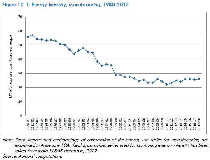 Average annual growth rates in energy intensity (based on physical measure of energy consumption) and the ratio of real value of energy input to real value of gross output are presented in Figure 10.2 for the sub-periods 1981-93, 1994-2002, 2003-10 and 2011-17. It shows that during 1981-82 to 1993-94 and 1994-95 to 2002-03, the average annual rates of growth were negative both for energy intensity and the ratio of value of energy used to gross output. In the sub-period 2003-04 to 2010-11, while the growth rate in energy intensity was negative, that for the ratio of value of energy to gross output was positive, indicating a mismatch. In the more recent period, 2011-12 to 2017-18, the rates of growth in both indicators were positive. Thus, the movements in the two series have some degree of similarity, and for the period 2011-12 to 2017-18, an upward trend is observed in both.160 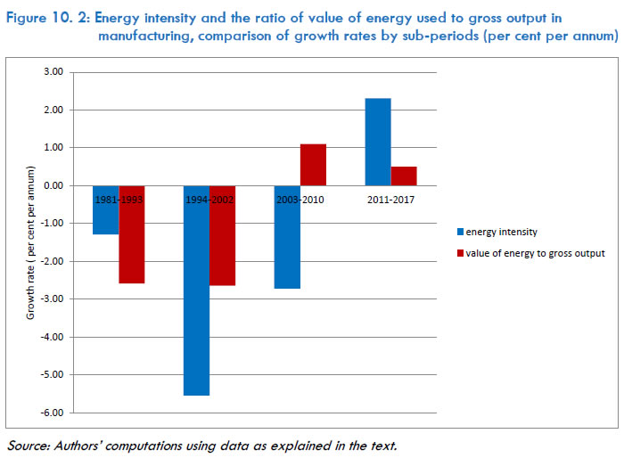 To further analyse the trends in recent years, we consider growth rates in energy use in manufacturing disaggregated by the types of fuel. Figure 10.3 depicts annual compound growth rates computed between the years 1993-94 and 2005-06, 2005-06 and 2010-11, and 2010-11 and 2017-18. Growth rate in real output in manufacturing during 1993-2005 (at 7.3 per cent per annum) was much higher than that in aggregate energy use in manufacturing (2.4 per cent per annum). While coal consumption grew at a rather low rate of about 1.2 per cent per annum during this period, the growth in consumption of petroleum products was relatively faster at about 2.8 per cent per annum. The annual growth rate in real output in the manufacturing sector increased to about 12 per cent during 2005-10, and this was accompanied by a hike in the annual growth rate in aggregate energy use in manufacturing to about 8.9 per cent during 2005-10. The annual growth in coal used by manufacturing increased from about 1.2 per cent during 1993-2005 to about 9.3 per cent during 2005-10. Petroleum product consumption accelerated likewise. Power consumption growth rose sharply from about 4.9 per cent per annum during 1993-2005 to about 11.8 per cent per annum during 2005-10. Yet, aggregate energy use in manufacturing during 2005-11 grew at a slower pace than real gross output, with the consequence that energy intensity in manufacturing fell during this period. 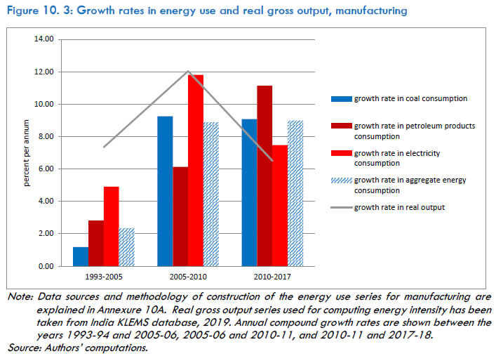 However, for the period 2010-17, the annual growth rate in real output in manufacturing fell substantively to 6.5 per cent from about 12 per cent during 2005-10. During the same reference period, the annual growth rate in aggregate energy consumption in manufacturing went up slightly from about 8.9 per cent to about 9.0 per cent. As a result, energy intensity in manufacturing increased.161 Interestingly, the growth rate in power consumption in manufacturing slowed in the latter period, whereas the growth rate of petroleum products consumption in manufacturing increased substantively. Indeed, in this period, there was substitution of coal and electricity by petroleum products in manufacturing, with the latter’s consumption growing annually at about 11.1 per cent during 2010-17. A more detailed examination of the energy use data reveals that this rapid growth in petroleum products in manufacturing was led by petroleum coke, the consumption of which grew at about 27 per cent per annum. According to energy sector media reports162, bulk of the petroleum coke consumption in Indian manufacturing takes place in the cement industry. Aluminium industry is another user of petroleum coke. 10.1.2 Trends in energy intensity in organised manufacturing In the next step, the trends in energy intensity in formal or organised manufacturing are considered (Figure 10.4). This analysis is based on data for the period 2004-05 to 2016-17 drawn from the Annual Survey of Industries (ASI)163. Annexure 10B provides details of computations of the associated energy use. There was a downward trend in energy intensity for the period 2004-05 to 2016-17 as a whole.164 This does not tally fully with the pattern observed in the analysis for manufacturing presented in the previous sub-section (Figure 10.1). Yet, one interesting point to be noted is that the energy intensity series for organised manufacturing based on ASI shows a significant fall between 2004-05 and 2011-12, but in the subsequent period, the fall was relatively rather small or marginal. In certain ways, therefore, this matches the pattern observed in Figure 10.1. 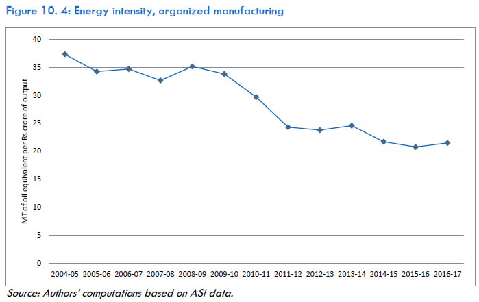 Table 10.1 shows the energy intensity in 13 India-KLEMS manufacturing industries in terms of averages for the years 2004-05 to 2006-07, 2010-11 to 2012-13 and 2014-15 to 2016-17.The table indicates that energy intensity is relatively high in the following industries or groups: Non-metallic Mineral Products (includes cement); Basic Metals and Fabricated Metal Products (includes basic iron and steel, and aluminium); Pulp, Paper, Paper Products, Printing and Publishing; Chemicals and Chemical Products; and Textiles, Textile Products, Leather and Footwear. In all these cases, there has been a fall in the level of energy intensity between the triennium ending 2006-07 and the triennium ending 2012-13; and between the triennium ending 2012-13 and the triennium ending 2016-17. | Table 10.1: Energy Intensity in Manufacturing Industries (Organized Segment) | | (MT of oil equivalent per Rs crore of output) | | Industry | 2004-05 to 2006-07 average | 2010-11 to 2012-13 average | 2014-15 to 2016-17 average | | Food products, beverages & tobacco | 15.30 | 10.93 | 9.84 | | Textiles & leather | 33.40 | 23.21 | 20.52 | | Wood & wood pdts. | 16.72 | 11.54 | 13.37 | | Pulp & paper pdts. | 64.37 | 46.95 | 42.78 | | Coke and petroleum pdts | 10.77 | 4.21 | 5.57 | | Chemicals & chemical pdts. | 35.21 | 28.65 | 25.29 | | Rubber & plastic pdts. | 32.70 | 11.93 | 9.87 | | Non-metallic mineral pdts. | 186.70 | 119.20 | 85.72 | | Basic metals & metal pdts. | 69.09 | 66.78 | 55.78 | | Machinery, n.e.c.. | 6.62 | 3.50 | 3.12 | | Electrical & optical eqpt. | 8.38 | 3.20 | 2.72 | | Transport eqpt. | 5.72 | 4.74 | 3.67 | | Other manufacturing | 2.40 | 1.41 | 1.32 | | All manufacturing | 35.40 | 25.92 | 21.32 | | Source: Authors’ computations based on ASI data. | Between the trienniums ending 2006-07 and 2016-17, energy intensity in aggregate organised manufacturing fell by about 40 per cent. The fall was relatively greater in Non-metallic Mineral Products (54 per cent). Other industries in which the fall was relatively large are Rubber and Plastic Products (70 per cent), Electrical and Optical Equipment (68 per cent) and Machinery n.e.c. (53 per cent). In contrast, the fall was relatively small in the case of Basic Metals and Fabricated Metal Products (19 per cent). To further understand the sources of change in energy intensity in aggregate organised manufacturing, a decomposition exercise was undertaken.165 It decomposed the change in energy intensity at the aggregate level into (a) structural change effect, (b) intensity effect and (c) residual. This analysis was done for two periods: (1) between 2004-05 and 2011-12, and (2) between 2011-12 and 2016-17. The results are presented graphically in Figure 10.5. Between 2004-05 and 2011-12, energy intensity of aggregate organised manufacturing fell by about 35 per cent. This was primarily caused by the intensity effect which was found to be (-)32 per cent and structural changes made a relatively much lower contribution as this effect was estimated to be (-)5.7 per cent. The residual term is 2.7 per cent. However, the subsequent period from 2011-12 to 2016-17 saw a smaller decline of about 12 per cent in energy intensity in aggregate organised manufacturing. While this period also saw a relatively larger attribution to lowering of energy intensity (estimated at (-)7.8 per cent) across industries, the structural change effect here is found to be (-)3.7 per cent, which plays a relatively more important role, and the residual term is (-)0.4 per cent. 10.1.3 Impact of energy prices on energy intensity in organised manufacturing The downward trend in energy intensity in manufacturing was observed till the end of 2000s. The energy intensity series for aggregate manufacturing shows a mild upward trend after 2010, whereas the energy intensity series for organised manufacturing based ASI data shows a marked slowdown in the downward trend after 2011. In this context, it would be pertinent to look at movements in energy prices. Between 2011-12 and 2017-18, there was a significant fall in the prices of several petroleum products. The price index for furnace oil fell by about 30 per cent and that for high-speed diesel fell by about 26 per cent. The price index for petroleum coke fell by 20 per cent between 2011-12 and 2015-16 and then recovered in the next two years; the index was higher in 2017-18 than that in 2011-12. The price index for electricity increased merely by 4 per cent in the six-year period from 2011-12 to 2017-18. However, the implicit price deflator for gross output in manufacturing increased by about 11 per cent between 2011-12 and 2017-18.166 These changes in petroleum product prices and the virtual stagnation in the electricity price index in the period 2011-12 to 2017-18, coupled with the fact that there was an increase in the price index for manufacturing sector output implies that there was a lowering of real price of energy in manufacturing (energy price divided by output price) during 2011-17, which could have been one of the important factors responsible for halting (or slowing) of the downward trend in energy intensity in manufacturing prevailing earlier. To substantiate this assertion, an econometric analysis of energy demand in organised manufacturing has been undertaken primarily directed at ascertaining the impact of energy price on energy demand. This analysis is presented in the next section. Besides energy price, the econometric models also include real gross output, capital intensity and the rate of growth in capital stock as explanatory variables. The level of energy use (or demand) is taken as the dependent variable in one of the estimated models and the level or rate of growth in energy intensity is taken as the dependent variable in the other models. | Lowering of real price of energy in manufacturing during 2011-17 could have been one of the important factors responsible for halting (or slowing) the downward trend in energy intensity in manufacturing. prevailing earlier | The key findings of the econometric analysis presented in Section 10.2 clearly show a significant negative relationship between energy price and energy demand in manufacturing (see also Annexure 10C). The estimated price elasticity of demand for energy emerging from the model estimates range from (-)0.8 to (-)1.3. The coefficient is found to be statistically significant. Thus, the results provide sufficient basis to infer that there exists an inverse relationship between real energy price and energy demand in manufacturing, and the fall in real price in energy that took place between 2011-12 and 2017-18 could indeed be an important factor that halted (or slowed) the downward trend in energy intensity in manufacturing prevailing earlier.167 10.2 Determinants Energy Use and Energy Intensity in Organized Manufacturing Econometric analysis of determinants of energy use and energy intensity in organised manufacturing has been undertaken using panel data at three-digit industry level (72 industries) for nine years, 2008-09 to 2016-17. Three models have been estimated. These are described below: Model 3 is similar to Model 2, except that lagged energy intensity is introduced as an additional explanatory variable. The equation has therefore been written as a dynamic panel data model. Models 1 and 2 have been estimated by the fixed effects model and Model 3 has been estimated by applying the difference and system GMM estimators. The results are shown in Tables 10.2, 10.3 and 10.4. | Table 10.2: Energy demand model, regression results (dependent variable: ln energy quantity) | | Explanatory variable | coefficient | t-value | | ln [real output] | 0.867 | 12.59 | | ln [real price of energy] | -1.186 | -10.49 | | ln [capital intensity] | 0.301 | 5.21 | | R-squared | 0.95 | | | No. of observations | 648 | | | F (prob.) | 31.0 (0.000) | | Note: Robust standard errors. Year dummies are included in the estimated model.
Source: Authors’ computations |
| Table 10.3: Model explaining energy intensity, regression results (dependent variable: change in logarithm of energy intensity) | | Explanatory variable | coefficient | t-value | | Change in logarithm of Real output | -0.331 | -4.83 | | Change in logarithm of Real price of energy | -1.300 | -8.72 | | Growth rate in fixed capital stock | 0.500 | 3.92 | | R-squared | 0.56 | | | No. of observations | 576 | | | F (prob.) | 39.1 (0.000) | | Note: Robust standard errors. Year dummies are included in the estimated model.
Growth rate in fixed capital stock = Gross fixed capital formation during the year as a ratio to closing fixed capital stock of the previous year.
Source: Authors’ computations |
| Table 10.4: Model explaining energy intensity, regression results (dependent variable: logarithm of energy intensity) | | Explanatory variable | Difference GMM (two-step method) | System GMM (two-step method) | | Change in logarithm of Real output | -0.236 (-5.33)*** | -0.241 (-3.81)*** | | Change in logarithm of Real price of energy | -0.874 (-6.01)*** | -0.894 (-7.34)*** | | Growth rate in fixed capital stock | 0.178 (2.03)** | 0.199 (1.88)* | | logarithm of energy intensity lagged one year | 0.384 (5.70)*** | 0.484 (6.67)*** | | Wald chi-squared and prob. | 619.1 (0.000) | 705.7 (0.000) | | No. of observations | 504 | 576 | | Sargan (chi-squared and prob.) | 33.0 (0.20) | 40.3 (0.21) | | AR(1), prob. | 0.001 | 0.001 | | AR(2), prob. | 0.355 | 0.310 | Note: Robust standard errors. Year dummies are included in the estimated model; t-ratios shown in parentheses.
Growth rate in fixed capital stock = Gross fixed capital formation during the year as a ratio to closing fixed capital stock of the previous year.
*, **, *** statistically significant at one, five and ten percent level, respectively
Source: Authors’ computations | The model estimates clearly indicate a negative effect of energy price on energy demand and energy intensity. The coefficient has plausible numerical value and is statistically significant at one percent in the estimates of all three models. The coefficient of real output is positive and statistically significant in the estimates of Model-1 (Table 10.2), with numerical value less than one. The coefficient is found to be negative in numerical value and statistically significant in the estimates of Models 2 and 3. This is suggestive of a less-than proportional relationship between real output and energy consumption at industry level. Energy consumption increases less than proportionately with growth in output. Thus, a high rate of growth in output leads to a fall in energy intensity. The estimates of Model-1 presented in Table 10.2 indicate a positive relationship between capital intensity and energy intensity. This is perhaps suggestive of a complementary relationship between capital input and energy input in the short run. The regression results presented in Tables 10.3 indicate that a high rate of new investment tends to raise energy intensity. The results reported in Table 10.4 are similar—the variable has a positive coefficient, and the coefficient is statistically significant. Thus, the results reported in Tables 10.3 and 10.4 indicate that a high rate of investment tends to raise energy use more than output and hence raises energy intensity. As a check of robustness of the regression results, the three models have been re-estimated after dropping the year dummies and replacing them by a quadratic trend term, i.e., a time variable169 and its squared term is introduced in the models. The regression results corresponding to Tables 10.2, 10.3 and 10.4 are given in Tables 10.5, 10.6 and 10.7. The results obtained by giving an alternate treatment to the time variable are similar to those in Tables 10.2, 10.3 and 10.4, and do not require much discussion. Suffice it to note that they indicate: (a) a negative effect of energy price on energy demand and energy intensity, (b) a less than proportionate effect of output growth on energy demand thereby lowering energy intensity, and (c) that a high rate of investment tends to raise energy use more than output and hence raises energy intensity. These findings are in line with those emerging from the results reported in Tables 10.2, 10.3 and 10.4. | Table 10.5: Energy demand model, regression results (dependent variable: ln energy quantity), alternate treatment of time variable | | Explanatory variable | coefficient | t-value | | ln [real output] | 0.866 | 12.31 | | ln [real price of energy] | -1.151 | -10.41 | | ln [capital intensity] | 0.298 | 5.24 | | Time | 0.0001 | 0.01 | | Time squared | -0.0012 | -0.57 | | R-squared | 0.95 | | | No. of observations | 648 | | | F (prob.) | 45.7 (0.000) | | Note: Robust standard errors.
Source: Authors’ computations |
| Table 10.6: Model explaining energy intensity, regression results (dependent variable: change in logarithm of energy intensity), alternate treatment of time variable | | Explanatory variable | coefficient | t-value | | Change in logarithm of Real output | -0.336 | -4.95 | | Change in logarithm of Real price of energy | -1.294 | -8.72 | | Growth rate in fixed capital stock | 0.519 | 4.28 | | Time | 0.061 | 2.34 | | Time squared | -0.0055 | -2.33 | | R-squared | 0.55 | | | No. of observations | 576 | | | F (prob.) | 70.5 (0.000) | | Note: Robust standard errors.
Growth rate in fixed capital stock = Gross fixed capital formation during the year as a ratio to closing fixed capital stock of the previous year.
Source: Authors’ computations |
| Table 10.7: Model explaining energy intensity, regression results (dependent variable: logarithm of energy intensity), alternate treatment of time variable | | Explanatory variable | Difference GMM (two-step method) | System GMM (two-step method) | | Change in logarithm of Real output | -0.231 (-5.65)*** | -0.247 (-3.85)*** | | Change in logarithm of Real price of energy | -0.816 (-7.32)*** | -0.863 (-6.57)*** | | Grgrowth rate in fixed capital stock) | 0.199 (2.65)*** | 0.210 (2.04)** | | Time | -0.166 (-4.24)*** | -0.111 (-2.86)*** | | Time squared | 0.011 (3.69)*** | 0.007(2.28)** | | logarithm of energy intensity lagged one year | 0.359 (5.22)*** | 0.481 (6.49)*** | | Wald chi-squared and prob. | 581.3 (0.000) | 504.4 (0.000) | | No. of observations | 504 | 576 | | Sargan (chi-squared and prob.) | 26.0 (0.52) | 39.9 (0.22) | | AR(1), prob. | 0.001 | 0.001 | | AR(2), prob. | 0.435 | 0.342 | Note: Robust standard errors.
*, **, *** statistically significant at one, five and ten percent level, respectively
Growth rate in fixed capital stock = Gross fixed capital formation during the year as a ratio to closing fixed capital stock of the previous year.
Source: Authors’ computations | The main finding emerging from the results of this econometric analysis presented above is that energy pricing has a significant effect on its demand and on energy intensity in organised manufacturing. Two other interesting findings emerging from the regression analysis are: (1) there is a less than proportionate effect of output growth on energy demand, and (2) a high rate of investment tends to raise energy use more than output and hence raises energy intensity. The implication of a less than proportionate effect of output growth on energy demand is that in a period of rapid growth in manufacturing sector output, there is a downward pressure on energy intensity. By that logic, as the growth rate of manufacturing sector output slows down, the downward pressure on energy intensity causing energy intensity to fall is no longer present. An interesting question examined next is how international trade impacts the energy intensity of Indian manufacturing. Several studies based on firm-level data have found that exporting reduces energy intensity (e.g., Batrakova and Davies, 2012; Jinji and Sakamoto,2015; Tran, 2021). Such findings have been reported also for Indian manufacturing in the studies undertaken by Martínez-Zarzoso et al. (2020) and Sahu et al. (2021). In a study undertaken of Indonesian firm, Imbruno and Ketterer (2018) have found that that as the share of imported materials in total materials consumed goes up, it reduces energy intensity. It would thus be interesting to examine the effects of exporting of products and importing of materials on energy intensity in Indian manufacturing using industry-level panel data which has been used for the analysis above. For carrying out this analysis, the mean export intensity (exports to production ratio) and the mean imported materials intensity (share of imported materials out of total materials consumed) has been computed for each three-digit industry for different years from 2009-10 to 2015-16 using the unit-level data of ASI. For computing the means, the sample weights have been used. The quantile regression method has been used for the econometric analysis. The dependent variable is the logarithm of energy intensity. The explanatory variables are the logarithm of real gross output, the logarithm of real energy prices, export intensity and imported materials intensity. The year dummies are included in the estimated model. The results are shown in Table 10.8. Estimates of the model have been made for the 50th percentile (the median) of the distribution of energy intensity, and for the 25th percentile and the 75th percentile. | Table 10.8: Energy intensity determination model, quantile regression (dependent variable: ln energy intensity) | | Explanatory variable | 25th percentile | 50th percentile | 75th percentile | | ln [real output] | -0.045(-2.05)** | -0.049(-2.59)** | -0.048 (-2.40)** | | ln [real price of energy] | -1.83(-15.82)*** | -2.10(-20.83)*** | -2.29(-21.50*** | | Export intensity | 0.05(0.10) | -0.32(-0.78) | -0.84(-1.94)* | | Imported materials intensity | -1.78 (-2.34)** | -1.22(-1.85)* | -1.35 (-1.95)* | | Pseudo R-squared | 0.34 | 0.40 | 0.48 | | No. of observations | 490 | 490 | 490 | *, **, *** statistically significant at one, five and ten percent level, respectively
Source: Authors’ computations | The results show a negative effect of energy price on energy intensity, which matches the results in Tables 10.2 to 10.7. The negative coefficient of the real output variable in the results reported in Table 10.8 is consistent with the results in tables 10.2 and 10.5. The results indicate that imports of materials reduce energy intensity. The coefficient is found to be negative and statistically significant. This is consistent with the findings of Imbruno and Ketterer (2018) in their study of the Indonesian firms. As regards exporting, a significant negative effect of export intensity on energy intensity is found for the 75th percentile of the energy intensity distribution, but not for the 50th and 25th percentile. It may thus be inferred that exporting tends to reduce energy intensity in high energy-intensive industries but not in low energy intensive industries. A similar finding for Indian manufacturing has been reported by Martínez-Zarzoso et al. (2020) who find that exporting has a negative effect on energy intensity among firms in the high energy-intensive industries but not among firms in the low energy-intensive industries. Similarly, Sahu et al. (2021), who have applied the quantile regression method to firm-level data, find that exporting has a negative effect on energy intensity among high energy-intensive firms but not among low energy-intensive firms. Clearly, the results reported in Table 10.8 is in line with the findings of Sahu et al. (2021). 10.3 Conclusion The chapter dealt with trends in energy intensity of Indian industries. The analysis of trends in energy intensity was presented for manufacturing and particular attention was paid to the organised manufacturing. The analysis of trends in energy intensity in manufacturing revealed a downward trend till the end of the 2000s, and a trend reversal or a slowing of the previously prevailing downward trend in energy intensity in manufacturing from 2011. Econometric analysis of determinants of energy use and energy intensity revealed a significant negative relationship between energy price and energy demand in manufacturing. An examination of movements in real price of energy revealed that there was a fall in real price of energy input in manufacturing in the period 2011-12 to 2017-18 and this could be one of the important factors that halted or slowed the previously prevailing downward trend in energy intensity in manufacturing. Other interesting findings are that a higher import intensity of materials is associated with a lower energy intensity and that exporting reduces energy intensity in highly energy-intensive industries. | There was a fall in real price of energy input in manufacturing in the period 2011-12 to 2017-18 and this could be one of the important factors that halted or slowed the previously prevailing downward trend in energy intensity in manufacturing. | Manufacturing accounts for a little over half of energy consumption of the Indian economy, and the finding that the previously prevailing downward trend in energy consumption in manufacturing ceased in the period 2011-17 (which could be an indication of the trends that have prevailed in the recent past and the likely trends in the coming years) is a matter of concern in view of India’s commitment to cut down its emissions intensity. Policy action is thus needed—particularly, a tax-subsidy policy that encourages manufacturing firms to cut down on energy use by substituting energy with other inputs or find technological solutions for energy conservation. One example already in operation for reducing energy intensity in energy-intensive manufacturing units is the PAT (Perform, Achieve, Trade) scheme. It successfully met its target in the first cycle (2012-13 to 2014-15) and lowered energy intensity by about 5.3 per cent in a period of three years, which was well above the initial target of about 4 per cent. Although the scheme continues to be in operation, given the subsequent trends in energy intensity in India’s manufacturing, it seems that the PAT scheme needs to be strengthened to have greater impact on energy intensity in manufacturing. With an appropriate policy of taxation that discourages high energy use and thus contains the resultant carbon emission, it may be possible to take advantage of international trade in boosting manufacturing value-addition in India without necessarily moving into energy-intensive manufactured products. This possibility needs to be explored. Perhaps, through greater integration into global value chains, it would be possible to increase GVA in manufacturing and employment without a proportionate increase in energy consumption (through changes in the products produced in the country and those traded). Annexure 10A: Construction of energy use and energy intensity series for manufacturing Computation of energy use in manufacturing takes into account the sector’s consumption of coal, power, natural gas, and various petroleum products including diesel oil, furnace oil, Low Sulphur Heavy Stock (LSHS), petroleum coke, and lubricants.170 Computation of total energy use for the purpose of constructing the energy intensity series is based on the concept of final use, i.e., the concept of ‘final consumption of energy commodity’ is used rather than ‘total primary energy supply’. Out of the total consumption of each specific petroleum products in the manufacturing sector, the part that is consumed by industry as feedstock (e.g., the consumption of naphtha in fertiliser and petrochemicals), rather than as fuel, is excluded. In other words, non-energy use of petroleum products and natural gas is excluded. Another point that should be noted here that auxiliary consumption in captive power plants in the manufacturing sector has been taken into account and treated as energy consumption in manufacturing. Data Sources on energy consumption Data on consumption for major energy sources (coal, lignite, electricity, natural gas, and petroleum products) in physical units have been taken from various official data sources. These include Indian Petroleum and Natural Gas Statistics, published by the Ministry of Petroleum and Natural Gas, Government of India, and Energy Statistics, published by the Ministry of Statistics and Programme Implementation, Government of India. For coal consumption, data have been drawn also from Provisional Coal Statistics and Coal Directory of India published by the Coal Controller’s Organisation, Ministry of Coal, Government of India. Data on electricity consumption, from utilities and non-utilities, and data on various other aspects of functioning of power plants have been taken from the publications of the Central Electricity Authority. Certain other sources which compile and report the official data on energy consumption have also been used. These include a CMIE (Centre for Monitoring Indian Economy) publication titled Energy. Conversion factors The conversion factors (for computing oil equivalent) are taken from diverse sources, including the Indian Petroleum and Natural Gas Statistics. For electricity, the conversion factor used is 1KWH = 0.00085 tonnes of oil equivalent. For natural gas, the conversion factor used is 1 Sm3 of natural gas = 0.00084 tonnes of oil equivalent. For various petroleum products, the conversion factors differ. For example, it is 1.130 for LPG, 1.075 for ATF, 1.035 for diesel oil, and 0.985 for residual fuel oil. For coal, the conversion factors used are 0.44 for domestically produced coal171 and 0.6 for imported coal (also for exported coal). For lignite, the conversion factor used is 0.23. Some adjustments made to official data Some adjustments have been made to the data on coal consumption provided in Energy Statistics published by the NSO (National Statistical Office). The coal consumption figures for the years 2004-05 to 2010-11 have been adjusted upward to take into account imports of coal. The sector wise distribution of total coal consumption for years 2009-10 onwards, particularly from 2014-15, has been modified by considering the sector-wise distribution of imported coal. For this purpose, the coal consumption data in power utilities as given by the Central Electricity Authority have been considered along with such data taken from the publications of the Coal Controller’s Organisation. Deriving energy use estimates for manufacturing For electricity, consumption data are available for the industry sector (which includes mining and quarrying) and not separately for manufacturing. Electricity consumption in mining and quarrying is relatively small compared with manufacturing, and therefore, no adjustment has been made to remove it. Electricity consumption data for industry has been treated as that for manufacturing. To derive coal consumption in manufacturing, coal consumption in power plants (utilities and non-utilities), households and the transport sector has been subtracted from aggregate coal consumption, and then in the next step, coal consumption in hotels and restaurants has been subtracted. The series thus obtained is treated as coal consumption in manufacturing. Domestic (i.e., household) consumption of coal for the years 1980-81 to 1983-84 has been taken from the official data. This has been extrapolated till 2016-17 using data on rural and urban population and percentage of rural and urban households using coal/coke as fuel for cooking taken from National Sample Survey Reports for different years (1983, 1993-94, 1999-2000, 2004-05, 2009-10, 2011-12). Consumption of coal in hotels and restaurants has been estimated with the help of data on expenditure on coal in different industries provided in input-output tables and supply-use tables. In the last 10 years, there has been a huge increase in the consumption of petroleum coke in the country, and at present among the petroleum products consumed in manufacturing, it greatly dominates over diesel, furnace oil and LSHS. Petroleum coke is used mostly in industries but is used also in power generation. Data are not available on sector-wise breakup of petroleum coke consumption (according to some media reports, the cement industry takes up about three-fourth of petroleum coke consumption in India), and no information could be gathered on what portion of petroleum coke supply is used as fuel in power plants. Therefore, the entire consumption of petroleum coke in the country has been treated as energy consumption by manufacturing. Annexure 10B: Construction of Industry-level energy use and energy-intensity series for organized manufacturing Industry-level energy intensity estimates have been made for organised or registered segment of manufacturing. The basic source of data is the Annual Survey of Industries (ASI) (Central Statistics Office, Government of India). The estimates have been made for the years 2004-05 to 2016-17. Estimates for 2008-09 to 2016-17 Estimates of energy use have first been made at three-digit industry level (NIC-2008), which have then been aggregated to obtain the estimates for the 13 manufacturing industries according to India KLEMS industry classification. In the published results of ASI, energy consumption data are provided for coal, electricity, and petroleum products, and other items are clubbed under the head ‘other fuel’. For coal and electricity, both quantity and value are provided. For this study, the value figures reported in ASI published results have been taken for each 3-digit industry for each year, and the quantities of coal and electricity used in the 3-digit industry have been derived by first computing median rate (i.e. price at which coal or electricity is purchased) among the factories belonging to the 3-digit industry using unit-level data (i.e. factory level data) and then dividing the value figure by the median rate. The quantities of coal and electricity so obtained have been multiplied by the conversion factors to derive oil equivalent. The figure on expenditure on petroleum products has been divided by the price of furnace oil to compute equivalent quantity of furnace oil which has then been multiplied by the conversion factor to derive the oil equivalent. The figure on expenditure on ‘other fuels’ reported in ASI has been divided into two parts: expenditure on natural gas and expenditure on other fuels. The relative share of natural gas has been computed (for each three-digit industry) from unit-level ASI data, and this has been used for splitting of the expenditure on ‘other fuels’ reported in ASI. The expenditure on natural gas has been divided by natural gas price (median rate computed at two-digit industry level using unit-level data of ASI and applied to all constituent three-digit industries) to derive quantity and then, by applying conversion factor, the oil equivalent has been obtained. After removing the expenditure on natural gas from the reported expenditure on ‘other fuels’ in ASI, the balance has been treated primarily as expenditure on fuel wood. Using price of fuel wood,172 the quantity figure has been derived and then, by applying the conversion factor, the oil equivalent has been derived. After deriving the quantities (in oil equivalent) of coal, electricity, petroleum products, natural gas and other fuels (treated predominantly as fuel wood) in each 3-digit industry each year according to the method explained above, these have been added to obtain the total quantity of energy use. The quantity of energy is divided by deflated gross value of output (at 2011-12 prices) to compute energy intensity. The 3-digit industries have been mapped into the 13 manufacturing industries according to India KLEMS classification, and then energy intensity in the 13 industries have been computed. The tables on fuels consumed in the published results of ASI are based on Block H of the schedule and thus do not take into account imported fuels/energy. For three industries, namely, Manufacture of Non-Metallic Mineral Products except glass and glass products (NIC 239), Manufacture of Basic Iron and Steel (NIC 241) and Manufacture of Basic Precious and Other Non-Ferrous Metals (NIC 242), imports of coal and coke have been taken into account and the energy use estimates have accordingly been adjusted for imported coal and coke.173 Estimates for 2004-05 to 2007-08 These estimates are based on the published ASI data on energy use by 4-digit NIC. The published data are used directly without making adjustments as done in the case of estimates for 2008-09 to 2016-17. One adjustment that has been made is to include imports of coal and coke in respect of Manufacture of Other Non-Metallic Mineral Products (NIC-2004, industry code 26) and Manufacture of Basic Metals (NIC-2004, industry code 27). Relative shares of fuelwood and natural gas within the category of ‘others’ are not available. Therefore, the shares for 2008-09 and 2009-10 for different KLEMS manufacturing industries have been considered, average shares have been computed for each industry, and these have then been applied to data for the years 2004-05 to 2007-08. Price of fuelwood for the years 2004-05 to 2007-08 has been derived from unit level data of ASI (as done for the estimates for 2008-09 to 2016-17), which has been used to compute the quantity of fuelwood used. The value of natural gas used has been divided by an appropriate price to derive the quantity of natural gas used. For this purpose, the average rate for natural gas across manufacturing industries has been computed for 2008-09. This has been extrapolated backward till 2004-05 by using the consumer price of natural gas for the years 2004-05 to 2008-09 provided in Indian Petroleum and Natural Gas Statistics. For each year, the value of natural gas consumed in various industries has been divided by the average rate for natural gas to compute the quantity of natural gas consumed in the industries. Annexure 10C: ARDL Model Estimation for Explaining Energy Intensity of Manufacturing using Time-series Data at the Aggregate Manufacturing Level An analysis of the impact of output, real energy price and capital intensity on energy demand has been undertaken in Section 10.2 in respect of organized manufacturing industries using a panel dataset at three-digit industry level (72 industries) for nine years, 2008 to 2016. In this annexure, a supplementary analysis is presented, based on a model using time-series data for aggregate manufacturing (i.e., both organised and unorganised segments are covered). The model is specified as: 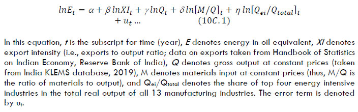 The above equation has been estimated by applying the Autor-Regressive Distributed Lag (ARDL) model. The equation is first estimated by using data for the entire period 1980 to 2017. These estimates are, however, not found satisfactory. The model results improve considerably when the estimation is done with data for the period 1980-2010. This seems to be an indication of a structural break in the relationship between energy intensity and its determinants around 2010. To verify this point, the estimated model for the period 1980-2010 has been used to predict energy intensity for the period 2011-2017, and a comparison is made with actual energy intensity. The estimated long run coefficients of the explanatory variables obtained from the estimation of the ARDL model are shown in Table 10C.1 and a comparison of actual energy intensity with the predicted energy intensity for the years 2000-2017 is presented in Fig. 10C.1. The coefficients of Q, M/Q and Qei/Qtotal (the share of energy intensive industries in aggregate manufacturing output) have the expected sign. | Table 10C.1: Determinants of energy intensity, ARDL Model Results, long-run coefficients | | Dependent variable: ln (energy/output) | | Explanatory variable | Period: 1980-2017 | Period: 1980-2010 | | ln XI | -0.67 (-1.90)* | -0.33(-7.78) # | | ln Q | 0.94 (4.68) # | 0.58(20.97) # | | ln M/Q | -0.44 (-0.47) | -0.44 (-6.05) # | | ln Qei/Qtotal | 1.67 (1.05) | 2.81(21.06) # | | Number of observations | 34 | 27 | | Lags | ARDL(1,0,0,0,0) | ARDL (4,4,4,4,3) | | R-squared | 0.21 | 0.99 | | F-value for bounds test | 1.5 @ | NA | | Source and note: Authors’ computations. t-values in parentheses, * statistically significant at the 10 percent level, # statistically significant at the 1 percent level, @ null hypothesis of no level relationship is not rejected. |
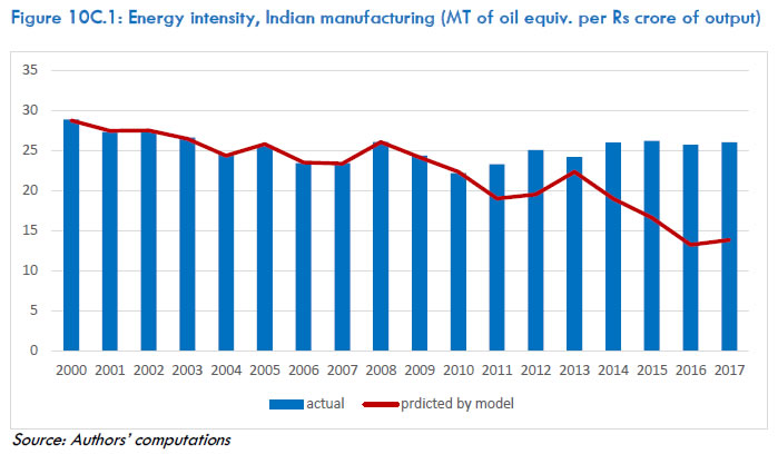 The nature of relationship that exists between trade and energy intensity of domestic industry has been investigated in the literature using economy or sector level data, and some studies have found a positive effect of trade on energy intensity. There are quite a few studies that have found a negative effect of exports on energy intensity. The results obtained from the econometric exercise undertaken for this study show that, in the case of India, exports had a negative effect on energy intensity of Indian manufacturing, i.e., a higher level of exports of manufactured products by Indian manufacturing industry would lead to improvement in energy use efficiency. The model estimated for the period 1980-2010 predicts the actual energy intensity for this period quite well. However, for predictions going beyond the sample period, it is found that the actual energy intensity is higher than that predicted by the model (Fig. 10C.1), suggesting that after 2010, there were certain forces at work other than the variables considered in the model which caused a halt to the downward trend in energy intensity of the manufacturing sector prevailing earlier, and led to a trend reversal. This is consistent with the analysis presented in Section 10.2 of the chapter. Chapter 11: Growth and Productivity in India’s Services sector 11.1 Introduction Understanding the drivers of economic growth is hugely beneficial for low-income countries like India as it is crucial to improving the living standards of their populations. Often productivity improvements in manufacturing industries are considered as one of the major sources of growth. This idea is analogous to the traditional structural transformation hypothesis that as a country develops, resources move from primary to manufacturing and subsequently to services (see Kuznets, 1966). The experience in India, however, seems to suggest that the country has been pioneering a stage of development that defies the conventionally hypothesised structural transformation. The Indian economy has been witnessing a service-driven growth, particularly since the 1990s, though it remains in the category of low middle-income emerging economies. While the share of services in India’s GDP has risen over much of the post-independence period, there was a marked acceleration in the trend since the early 1990s. Similarly, the relative importance of the services sector in employment generation has also increased substantially. Moreover, the export share of services has been large and increasing in recent years (Eichengreen and Gupta, 2012). The economic reforms of the 1990s, which paved the way for trade liberalisation, along with major policy changes in the domestic business environment may have helped the emergence of the service sector as a key player in India’s growth story. Traditionally, services have been a regulated activity. This was particularly true in areas of banking, insurance, and telecommunication, which are among the industries that witnessed massive improvement in the post-reform period. Further, this sector has evolved as a prominent one in terms of contribution to national and state incomes, trade flows, FDI, and employment. The emergence of services as the most dynamic sector of the Indian economy has in many ways been a revolution. The most visible and well-known dimension of the take-off in services has been in software and information technology (IT)-enabled services (including call centres, software design, and business process outsourcing), which to some extent also help increase innovation capabilities in the sector (Lema et al., 2012). However, growth in services in India has been much more broad-based than IT (Gordon and Gupta, 2004). There have been many studies looking into India’s service-driven economy (Eichengreen and Gupta, 2009, 2010), and its sluggish manufacturing. While studies on structural transformation suggest that the observed structural transformation in India has been growth enhancing (McMillan and Rodrik, 2011; Bosworth and Collins, 2008; Vries et al., 2012), evidence on services sector suggests that the observed growth surge is mainly due to higher productivity growth in this sector (Verma, 2012). However, there has hardly been any attempt to explain the observed momentum in the service economy in detail, particularly by looking into how productive the sector is and what are the factors that drive its productivity. This chapter attempts to revisit the “services-led growth” hypothesis for the Indian economy by undertaking detailed analysis of the service industries in terms of labour productivity and multifactor productivity growth. An attempt is made to explore the factors that drive productivity performances in the sector. Yet another aspect that has been overlooked in the literature is the complementarities between service sector growth and manufacturing performance, which calls for understanding why productivity improvement in the manufacturing sector continues to be sluggish. Examination of the above issues constitutes the core of this chapter. | This chapter attempts to revisit the “services-led growth” hypothesis for the Indian economy by undertaking detailed analysis of the service industries in terms of labour productivity and multifactor productivity growth. | To understand the empirics of India’s growth performance, we undertake a growth accounting exercise based on the KLEMS production function approach due to Jorgenson, Gollop and Fraumeni (1987). The gross output production function incorporating KLEMS as inputs allows us to evaluate the relative significance of multifactor productivity growth vis a vis input accumulation in accounting for output growth. Using the newly created comprehensive India KLEMS dataset version 2019 for the Indian economy for the period 1980-2017, we compute productivity trends for the service sector. The chapter analyses sources of labour productivity in ten subsectors of the service economy—trade, hotels and restaurants, transport and storage, post and telecommunication, financial services, business services, public administration, education, health, and other services. These ten subsectors are further reclassified into market services and nonmarket services, within which we also examine ICT intensive and non-ICT intensive service segments separately. This chapter makes several contributions to the existing literature. First, in contrast to previous productivity studies in the Indian context, we use additional measures of factor inputs, which will have important consequences for productivity analysis (see OECD, 2001, Productivity manual). Both labour and capital inputs are measured as Tornqvist indices of different types of workers and asset types. Labour input, which is inclusive of self-employment, is measured using five education categories of employment, with the growth of each category being weighted by its relevant cost share. In the case of capital input, previous studies have used a measure of capital stock, often making no adjustment for depreciation of various asset types. Such an approach ignores the importance of heterogeneity in capital assets due to the existence of multiple vintages and various asset types. In our analysis, we use a measure of capital services using three different asset types, asset-specific depreciation rates and an external rate of return (see Diewert, 2003; Schreyer, 2002). Our second contribution is in providing a detailed sectoral perspective on India’s service sector. Since there is substantial heterogeneity within the sector, and the contribution of its different segments to aggregate service sector growth is substantially different, we examine the productivity dynamics of the service sector at detailed industry level. Our detailed focus also helps in understanding the respective position of market services as against nonmarket based services, and ICT using and producing services as against non-ICT services in the overall service sector performance in India. Third, at an industry level we use a gross output production function, which includes contribution of intermediate inputs in the production accounts. The period of the study pertains from 1980-81 till 2017-18 and is split into four distinct sub-periods of the Indian economy. We adopt the classification provided by Panagariya et al. (2014)174 as period 1 (1981-93)—a period where India’s per capita GDP grew at an average annual rate of 2.9 per cent. The second period consists of years 1994-2002, during which India’s per capita GDP grew at an annual rate of 3.9 per cent. Additionally, we look at the ‘golden growth phase’ of 2003-07. The final period looks at the global slowdown phase from 2008-17 when the per capita GDP growth declined. | Given the substantial heterogeneity within the service sector, and the variation in contribution of its different segments to aggregate service sector growth, we examine productivity dynamics at the disaggregated industry level | The chapter is structured as follows. Following the introduction, Section 11.2 provides an overview of the service sector liberalisation by providing a pre-reform context followed by the major reforms and a brief discussion on the impact of said reforms. Section 11.3 looks at the service sector performance over the entire sample period of 1980-2017 and the above-mentioned sub-periods, with a focus on Gross Value Added (GVA) and employment. Trends in productivity in the services sector are analysed in Section 11.4. Using a value-added framework, we decompose the sources of observed labour productivity growth while the role of TFP versus factor inputs is addressed via the gross output-based KLEMS framework. The final section concludes the chapter. 11.2 Service Sector Liberalization: An Overview A proper appraisal of the performance of India’s service sector should be preceded with an overview of the policies and reforms that have governed this sector. Post-World War II, India had been historically known to be one of the most regulated economies at the time. Inward looking policies and the “license-raj” constrained the economy to a very low growth path. This historical trend was later overturned through a series of liberalisation policies that brought an end to the excessive governmental monopoly and regulation, including tariff reductions and deregulation in many sectors. The service sector remained largely state-dominated before the early 1990s due to a variety of restrictions on foreign and private domestic players. Telecommunication services were solely provided by the Department of Telecommunications (DoT) till the entry of licensed private players started in 1992. The banking sector witnessed nationalisation of large private sector banks in 1969, leading to public sector dominance complemented with a host of regulations (credit direction, interest rate determination by the government etc.). The sector became vulnerable to moral hazard as banks expected government bailout in case of failure (Reddy, 2004). The banking sector would later undergo liberalisation under the RBI in 1994 with the aim of increasing efficiency and competition. Prior to the 1990s, transport services were also subject to public sector dominance in the form of public monopolies in air transport, state control over ports, registration requirements for different vehicle types and a variety of other regulations. The insurance sector was mainly operated by four public sector entities under the Ministry of Finance with negligible private competition before the reforms of mid 1990s. To put things in perspective, Figure 11.1 shows the trend followed by gross output and value added of the service sector (at 2011-12 prices) over the 1980-2017 period. It is observed that both these variables remained stagnant in the pre-reforms period, while there was a clear upward trend starting from the early 1990s—a period of service sector liberalisation. | Gross output and value added of the service sector remained stagnant in the pre-reforms period, while there was a clear upward trend starting early 1990s—a period of liberalisation for the sector | Hoekman et al. (2007) point out that the pace of reforms in different sectors was mainly determined by political considerations—sectors that would face large-scale transformation following liberalisation saw a slower pace of reform than the sectors that were flexible enough to accommodate greater competition without lowering profits or employment. Within the sectors that have been liberalised, public sector incumbents have remained competitive with a stake in the growing market—for example, -MTNL and BSNL have remained as major telecom providers in the telecommunication sector, a sector which saw large-scale removal of restrictions in the early 1990s. Table 11.1 provides a comprehensive summary of major reforms in the services sector. 
| Table 11.1: Major reforms/milestones of India’s service sector liberalization | | Year(s) of achievement/ Sector | Major reforms/milestones | | Telecommunications 1994 | Introduction of National Telecom Policy (NTP) paved the way for systematic liberalisation of the sector. | | 1997 | TRAI, an independent statutory regulatory body is set up; Entry of private participants in a duopoly basis; Rationing of Licenses; Foreign equity participation in mobile services permitted up to 49%. | | 1999 | New NTP introduced with the stated commitment to independent regulator and clear definition of TRAI’s role; licensing fee made more favourable for private operators. | | 2000-04 | National and International long-distance telephony opened to private players; removal of restrictions on the number of operators; disinvestment of public sector telecom providers in some metros. | | 2005 | Foreign holding limit raised from 49% to 74%; FDI permitted up to 100% in value-added services; greater flexibility to existing and reductions in entry and licensing fee shares. | | Banking 1993 | RBI allowed entry of private sector banks; FDI up to 20% allowed; banks given more freedom to allocate their inventories and receivables. | | 1996 | Guidelines issued for setting up private local area banks. | | 2000-01 | Discretionary barriers to entry are lowered; 40% limit for non-resident participation and associated borrowers from overseas increased to 49%. | | 2001-02 | Above mentioned limit is raised to 49% from all RBI’s automatic route; Interest rate deregulation allowed banks to set prices freely. | | 2004-05 | Above mentioned limit is raised to 74%; foreign banks allowed to operate through branches, fully owned subsidiaries and subsidiaries. | | Transport 1993-94 | Public monopoly in domestic air services abolished; prices in maritime freight and passenger transport liberalised. | | 1997-98 | FDI up to 40% allowed in air transport (foreign airlines excluded); Private sector engagement in road infrastructure with the ‘Build, Operate, Transfer’ scheme; Majority FDI allowed in construction and operation of ports. | | 2004-05 | Private airlines allowed to serve international routes; increased competition for public sector airlines from private players. | | Insurance 1999 | Insurance Regulatory and Development Authority (IRDA) Bill formally liberalised the sector to allow private entry; foreign equity participation up to 26% allowed; Pricing freedom given with supervision. | | 2000 | IRDA constituted as a statutory body; sector opened up to private and foreign players with 26% foreign ownership. | | 2002-03 | Entry of 12 new private players put pressure on the incumbent insurance providers. | | 2015 | Foreign investment cap increased from 26% to 49% under the Insurance Laws (Amendment) Bill. | | Health 1990s | Limited decentralization of healthcare system allowed some local governments more control over resource allocation; introduction of user- fees under the eighth five-year plan (1992-97); paradigm shift with focus on delivery to underprivileged groups. | | 2000s | Contracting out of health services to private providers; increased geographic coverage; introduction of public-private mix. | | Education 2000 | Foreign equity participation allowed up to 100% for entry through franchises, twinning arrangements, study centres and programme collaboration; 49% foreign equity participation for research and teaching activities; regulatory environment requires establishing entity to be non-profit. | | 2010 | Introduction of the Foreign Educational Institutions Regulation of Entry and Operations Bill under UPA-II for allowing foreign education providers to offer degrees and diplomas to Indian students, however, the Bill would later lapse. | | 2016 | Proposal by the Commerce Ministry to allow foreign universities to set up campuses in SEZs, however, the idea was not supported by the HRD ministry. | | 2019 | ‘Internationalisation’ included as a focus under the five-year plan of the HRD ministry called Education Quality Upgradation and Inclusion Programme; ideas to revisit the Foreign Education Bill previously introduced under UPA-II. | | 2020 | National Education Policy (NEP) approved by Union Cabinet with the vision to restructure the education system from elementary to higher education by the year 2040. | | Source: Authors compilation based on J.M. Arnold et al. (2016) & R. Chanda and Pralok Gupta (2011). | On a more conceptual level, the different policy aspects governing the service sector in India can be categorised into: (1) general issues and (2) sector-specific issues. General issues are broadly connected with foreign direct investment (FDI), tariff and taxes, credit and finance. Additionally, issues connected with domestic regulation, market access, bilateral and multilateral negotiations are significant policy issues when addressing reforms in the Indian service sector. Major sector-specific issues are primarily connected with the level of permissible FDI and thereby the extent of foreign competition allowed. Prasad and Sathish (2010) provide comprehensive analysis of the policies undertaken in the service sector in recent years (see Table 11A.1 of Annexure 11A). To take a few examples, entry of foreign firms through partnerships/joint ventures in insurance firms and through FDI in health insurance has characterised the banking and insurance sector in recent times. In the banking sector, though foreign investment cap of 74 per cent is allowed, issues remain regarding licensing requirements, etc. Healthcare has no FDI cap, but there remain barriers on foreigners providing medical services for profit. Education services in India come under the jurisdiction of both state and federal governments and there are regulations on setting up of new education services in some fields such as medicine. Thus, as it stands now, there are regulators for some services (banking, insurance, telecom, and ports), whereas most professional services lack independent regulators resulting in unevenness of standards across professional services.175 The large-scale liberalisation measures have shown a positive impact in the contribution of services to India’s trade flows. Figure 11.2 below shows that services accounted for 51.7 per cent of India’s gross exports in 2015 (OECD-TiVA, 2018), although this is lower than the OECD average of 54 per cent. Despite the impressive performance of services trade in India, it is important to note that exports of services remain constrained by domestic and external barriers (infrastructure, technical, standards financial) and regulatory aspects. 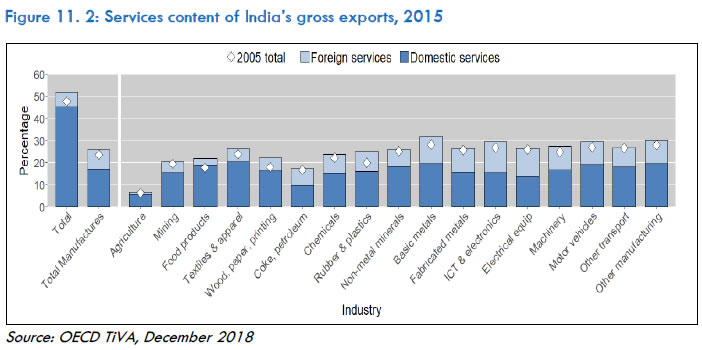 It is also important to keep in mind that the service sector provides crucial inputs to other sectors and hence generating more efficiency in the services sector via policy reforms could enhance competitiveness in the overall economy. Nowhere is this truer than for the manufacturing sector i.e., an efficient service sector is an important precursor for manufacturing competitiveness. Figure 10.2 shows that services value added accounted for around 25 per cent of total manufacturing exports in 2015. There are several studies in the context of services-manufacturing linkages, for example, Arnold et al. (2016) used firm level data for India and found a positive link between services liberalisation and performance (TFP) of manufacturing industries. 11.3 Service Sector Performance: 1980-2017 Unlike the East Asian model, the service sector played a predominant role in the transformation of India from its “Hindu rate of growth” phase to one of the fastest growing countries in the world. This unique feature of the Indian economy makes detailed analysis of the service sector a pertinent topic in the literature. In what follows, we first discuss some of the basic concepts of the service sector in the Indian context. This is succeeded by the reforms and policies that have been aimed at this sector. We end this section by giving an overview of the performance of the service sector in India and comparing it with the traditional driver of economic growth—manufacturing. The service sector encompasses a plethora of diverse and heterogeneous economic activities. It is for this basic reason that it has become increasingly difficult to give a precise definition to the activities pertaining to this sector. In India’s National Accounts Statistics, the sector consists of: wholesale and retail trade, hotels and restaurants, transport services, storage services, communication services, financial services, real estate, ownership of dwellings and renting services, business services and other social, community and personal services. In terms of measurement, it is probably more difficult to measure than goods, as services often represent a process by which a consumer is charged—hence there are conceptual problems in both “quantity” and “quality” of services (Melvin, 1995), as well as determining the price of the service. For collection of data and analysis, the subsectors are further categorised into public, private organised, and private unorganised. The public sector estimates of gross value added are obtained from data on output and intermediate outputs from budget documents. For some sectors of the private organised segment and most of the private unorganised segment, value added is computed using the ‘labour input’ method—multiplying the estimates of value added per worker in a benchmark year with the estimated labour force from census surveys (Nayyar, 2012). However, each of the methods of measurement has its own problems. Given that the output of service sector is often measured in terms of employee compensation, an increase in wages would imply an increase in real output even with the same actual activities. On the other hand, the quality of the crucial components of the ‘labour input’ method—estimates of the workforce and estimates of value added per worker—are quite low (Tendulkar, 2007). Lastly, the lack of a suitable service sector price index depletes the precision of constant price estimates of this sector. With these limitations and concepts in mind, it is interesting to ascertain the role of the service sector as the primary driver of India’s growth performance. Table 11.2 provides a comprehensive analysis of its contribution to Gross Value Added (GVA) and employment. It shows services contribution to GVA at around 54 per cent per annum in 2017 compared with 37 per cent in 1980, with market-based services as the largest component with a share of 32 per cent in 2017. Within market services, ICT-intensive services considerably dominated ICT-non intensive services in terms of GVA share, for each decade of the study period. At the outset, it may be argued that the growth in services can be attributed to increase in relative prices or to a result of outsourcing of activities (or splintering), causing the growth of final demand for industrial or agricultural products to raise the share of services in GDP. Yet, the data does not indicate any of these arguments holding true—implicit GDP price deflators during 1993-2010 did not increase noticeably. Moreover, increase in the use of services inputs by other sectors over time cannot explain the recent surge in the growth of the services sector (Gordon and Gupta, 2004; Nayyar, 2012). Thus, services growth in India was real rather than a statistical artifice. Unlike agriculture, services contribution to employment remains low and non-commensurate with the movement in services’ share in GVA. Yet we find a consistent upward movement as far as “jobs in service sector” is concerned from 17 per cent share in total employment in 1980 to 34 per cent in 2017. Similar to the case of value added, we find that the employment share of market services (22 per cent) exceeded that of non-market services (12 per cent), with a higher share of ICT-intensive services (15 per cent) over ICT non-intensive services (7 per cent), in 2017. There may be various reasons for the low employment absorption in the overall services sector relative to its share in GVA. Nayyar (2012) finds that educational requirements vary across different subsectors in the service sector and manifests itself through low quality of employment. | Unlike agriculture, services’ contribution to employment remains low and non-commensurate with the movement in services’ share in GVA. Variation in educational requirements across services might be manifesting as low quality of employment |
| Table 11.2: Relative contribution of services industries to gross value added and employment share | | | 1980 | 1990 | 2000 | 2010 | 2017 | | Description | GVA share | EMP share | GVA share | EMP share | GVA share | EMP share | GVA share | EMP share | GVA share | EMP share | | All Services | 36.77 | 16.94 | 40.30 | 19.98 | 46.57 | 24.33 | 48.55 | 28.67 | 53.50 | 33.80 | | Market Services | 15.19 | 9.12 | 18.76 | 11.81 | 25.39 | 15.14 | 28.39 | 18.52 | 32.09 | 22.18 | | ICT Intensive Services | 11.29 | 6.43 | 13.64 | 8.33 | 19.38 | 10.63 | 22.54 | 12.81 | 26.27 | 15.24 | | Trade | 6.92 | 5.80 | 7.45 | 7.34 | 8.49 | 9.08 | 9.42 | 10.02 | 10.85 | 10.91 | | Financial Services | 2.65 | 0.31 | 3.38 | 0.51 | 4.79 | 0.57 | 6.03 | 0.91 | 5.44 | 1.13 | | Post and Telecommunication | 0.75 | 0.14 | 1.17 | 0.18 | 1.97 | 0.33 | 1.56 | 0.38 | 1.56 | 0.39 | | Business Services | 0.97 | 0.18 | 1.63 | 0.30 | 4.13 | 0.65 | 5.53 | 1.50 | 8.42 | 2.82 | | ICT non-intensive services | 3.90 | 2.70 | 5.13 | 3.49 | 6.01 | 4.50 | 5.85 | 5.71 | 5.82 | 6.94 | | Hotels and Restaurants | 0.58 | 0.80 | 0.68 | 0.91 | 0.95 | 1.17 | 1.06 | 1.64 | 0.99 | 1.95 | | Transport and Storage | 3.32 | 1.90 | 4.45 | 2.57 | 5.06 | 3.34 | 4.78 | 4.06 | 4.83 | 4.98 | | Non-Market Services | 21.58 | 7.81 | 21.54 | 8.16 | 21.18 | 9.19 | 20.16 | 10.15 | 21.41 | 11.62 | | Public Administration & Defence; Compulsory Social Security | 5.20 | 2.75 | 6.00 | 2.84 | 6.70 | 2.47 | 6.15 | 1.79 | 6.17 | 1.70 | | Education | 1.96 | 1.58 | 2.34 | 1.62 | 3.10 | 2.15 | 3.30 | 2.95 | 4.12 | 3.77 | | Health and Social Work | 0.84 | 0.58 | 1.04 | 0.56 | 1.35 | 0.72 | 1.43 | 0.97 | 1.69 | 1.29 | | Other services | 13.59 | 2.90 | 12.15 | 3.14 | 10.03 | 3.86 | 9.27 | 4.44 | 9.43 | 4.87 | | Source: Authors’ computation from National Accounts Statistics, Government of India, and India KLEMS database, 2019 | Given the variety of economic activities that the service sector encompasses, it is worth looking at the trends at the subsector level. We observe from Figure 11.3 that service sector growth is widespread across various activities. In accounting for growth in value added in different subsectors, we find that business services show the maximum growth (around 12 per cent per annum), for the 1981-2017 period. If we consider the period of 2003-07, we find post and telecommunications and business services exhibiting high growth rates of around 11 per cent and 13 per cent, respectively. The telecommunication liberalisation began in 1994 with the private sector being allowed to offer telecom services. The rapid innovation in IT makes it a dynamic contributor to the growth of the Indian economy by itself (Singh, 2014). The domestic IT and hardware market has also become substantial in size and scope, although the value added for the latter is probably less than software and ITES. On the contrary, the employment generating potential of service sector in India has been the subject of intense debate on sustainability of service sector growth in India. Issues related to skilled versus unskilled nature of labour force requirements have been at the core, based on access to education and training. A glance at the panel B of Figure 11.3 shows that financial services and business services have been the major providers of employment, for the 1981-2017 period. Further, majority of the sectors show an employment growth of around 3 per cent for the period of 1981-2017. 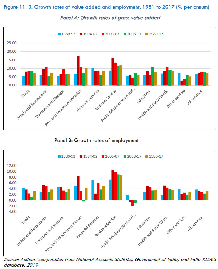 While there is a broad agreement about the dynamism of the service sector, questions have been raised about the sustainability of services growth (Acharya, 2002; Bosworth, Collins & Virmani, 2007; Panagariya, 2008). Singh (2006A) argues that services had proportionately the largest inducing effect in terms of backward linkages as well as forward linkages (albeit weaker than backward linkages). These linkages, the author argues, had an important impact in the reduction of transaction costs during the 1980s and 1990s and subsequently stimulated the entire economy to an extent. Moreover, introduction of a range of rural ICT services (ICTS) provides spillovers from ICTS through knowledge acquisition and information access (Singh (2006B)). Several policy implications emerge from the analysis—tackling education and technological bottlenecks and some labour market reforms that improve the innovation capabilities in the economy can go a long way to solve the problems of the service sector to increase its scope and labour absorption abilities, while continuing to remain dynamic for leading India’s economic growth. We need to infer if the driving force behind the service sector growth in India can be explained through improvements in resource use efficiency (both labour and total factor productivity growth). The rest of the chapter will make an attempt in this direction.176 11.4. Productivity Trends in India’s Service Sector Several empirical studies (Balakrishnan and Parameswaran, 2007; Bosworth et al., 2007; Rakhsit, 2007; Bosworth and Maertens, 2010) have identified the service sector as the driver of India’s economic growth. Using growth accounting tools, some of the studies also analysed whether such observed growth was led by efficiency of resource use (TFP) or input accumulation. Nayyar (2012), however, argues that such studies are only at the aggregate level and hence do not take into account any intra-industry group differences within services. These differences could arise because of structural characteristics—(i) organised-unorganised, (ii) intermediate-final, and (iii) public-private. In addition, these industries differ due to barriers to entry for job seekers, technology in use, and factor use — (1) capital intensity and (2) skill intensity. Therefore, it is essential that we figure out the channel via which growth is taking place across these industries — Growth through increases in capital accumulation or through employment expansion or even some sectors in unorganised services boosting growth by employing unskilled workers.177 The present empirical analysis is thus an attempt towards recognising that service industries are heterogeneous in several respects and, thereby, a disaggregated industry level perspective is needed to understand productivity—both labour and multifactor as well as the role of productivity in explaining overall growth in services. | Our measure of labour input incorporates qualitative aspects of the labour force in terms of education while defining a new measure of labour input as the product of labour person and the quality index. The capital input defined in terms of capital service takes asset heterogeneity into account. | In this section, we provide estimates of labour productivity growth using a value-added framework for various subsectors of services in India. Using this approach, we also detail the sources of labour productivity growth. Measurement and analysis of productivity at the disaggregate as well as aggregate levels, when based on the value-added version of the production function, ignores the explicit role of intermediate inputs in the production process. In the present chapter, we have considered three intermediate inputs—energy, material, and services, and this is important as we may find that intermediate inputs are the primary component of some industries’ outputs.178 Failure to quantify intermediate inputs leads us to miss both the role of key industries that produce intermediate inputs and the importance of intermediate inputs for the subsectors that use them (Jorgenson, Ho and Stiroh (2005), Productivity, volume 3). Our measure of labour input incorporates qualitative aspects of the labour force in terms of education while defining a new, refined measure of labour input as the product of labour person and quality index. The capital input defined in terms of capital service takes the asset heterogeneity into account as against a measure of capital stock which is devoid of it. In the following subsections, we discuss the estimates and sources of labour productivity and output growth using the value added and gross output version of the production function, respectively. Sources of Labour Productivity Growth The service sector’s performance in terms of labour productivity is summarised in Table 11.3. Our main observation is that labour productivity in India’s service sector has been growing substantially over the decades of the study period, and much of this productivity gain is accruing through acceleration in non-market services productivity. In the pre-reforms phase (1981-93), non-market services showed higher labour productivity growth relative to market services, with the opposite happening in the reform phase (1994-02) and the golden growth phase (2003-07). However, market services fell behind non-market services in terms of labour productivity growth in the global slowdown phase (2008-17). A closer examination further suggests that ICT intensive sectors, in particular trade and post & telecommunication have driven much of the market services productivity growth, while non-market services growth has been led by public administration. For the entire study period, labour productivity in services grew at the rate of close to 4 per cent per annum. Turning attention to the individual industries within services, we find that a majority shows labour productivity growth lower than the sectoral average, the exceptions being post and telecommunication, public administration, and health and social work which register high labour productivity growth in the region of 5 to 6 per cent. | Table 11.3: Labour productivity growth in service industries by subperiod: 1981–2017 (% per annum) | | Description | 1981-93 | 1994-02 | 2003-07 | 2008-17 | 1981-17 | | All Services | 2.89 | 4.41 | 4.97 | 5.43 | 4.23 | | Market Services | 1.72 | 4.91 | 5.38 | 4.71 | 3.80 | | ICT Intensive Services | 1.85 | 5.69 | 5.08 | 4.91 | 4.05 | | Trade | 1.19 | 4.35 | 5.89 | 6.97 | 4.16 | | Financial Services | 3.22 | 6.31 | 2.61 | 2.55 | 3.71 | | Post and Telecommunication | 1.73 | 9.14 | 7.86 | 7.43 | 5.90 | | Business Services | 1.64 | 5.48 | 3.82 | 2.29 | 3.04 | | ICT non-intensive services | 1.25 | 2.47 | 6.23 | 3.65 | 2.87 | | Hotels and Restaurants | 2.95 | 4.49 | 5.92 | 2.36 | 3.57 | | Transport and Storage | 0.97 | 2.13 | 6.31 | 3.94 | 2.78 | | Non-Market Services | 3.61 | 3.19 | 3.55 | 6.00 | 4.14 | | Public Administration and Defence; Compulsory Social Security | 3.80 | 6.52 | 6.45 | 7.91 | 5.93 | | Education | 3.30 | 3.62 | 1.23 | 7.43 | 4.21 | | Health and Social Work | 5.21 | 3.42 | 6.31 | 5.11 | 4.90 | | Other services | 3.22 | 0.71 | 1.20 | 3.97 | 2.54 | | Source: Authors’ calculations based on India KLEMS dataset version 2019 | The disaggregated picture in Table 11.3 offers a few interesting observations: Four market services sectors—hotels and restaurants, post and telecommunications, trade and transport and storage showed large improvements in productivity from a very low base in the decade of 1980s. All the service industries mentioned above had significant changes in their business environment beginning from the 1990s covering regulation as well as policy measures. For road transport, we find reforms from early 1990s covering entry of private players, amendments in motor vehicle laws, setting up of National Highways Act. Domestic air transport was liberalised in 1993 with the monopoly of Indian Airlines’ being abolished, leading to greater competitive pressure in domestic air services. In the case of telecom services, most manufacturing services were completely under governmental domain and private firms were allowed to provide telecommunication services in 1992 with the introduction of cellular service licences. In 1994, the government announced a new National Telecom Policy that provided guidelines for the private sector’s involvement. In financial services, especially banking, substantial reforms were undertaken pertaining to new banks and licensing policies. In 1993, the government issued guidelines for allowing entry of new private banks, although approvals remained difficult due to stringent RBI regulations. Reforms in the insurance sector commenced in the latter part of 1990s and securities markets were also streamlined. Next, we look at the contribution of individual industries to aggregate labour productivity growth in the service sector for the period of 1981-2017. The aggregate productivity growth is the weighted sum of industry productivity growth plus a reallocation term R. The reallocation term is positive if value added shifts from low productivity industries towards high productivity industries. Table 10.4 summarises the contributions of major service groups (market services—ICT and non-ICT intensive, and nonmarket services) and reallocation effect to labour productivity growth in the service sector. | Table 11.4: Industry contributions to aggregate labour productivity growth by subperiod; 1981-2017 | | Description | 1981-93 | 1994-02 | 2003-07 | 2008-17 | 1981-17 | | All Services | 2.89 | 4.41 | 4.97 | 5.43 | 4.23 | | Market Services | 0.74 | 2.59 | 3.05 | 2.72 | 2.04 | | ICT Intensive Services | 0.58 | 2.27 | 2.21 | 2.29 | 1.67 | | Trade | 0.22 | 0.83 | 1.14 | 1.39 | 0.81 | | Financial Services | 0.25 | 0.69 | 0.30 | 0.29 | 0.38 | | Post and Telecommunication | 0.05 | 0.39 | 0.34 | 0.27 | 0.23 | | Business Services | 0.06 | 0.36 | 0.43 | 0.34 | 0.26 | | ICT non-intensive services | 0.16 | 0.32 | 0.84 | 0.43 | 0.37 | | Hotels and Restaurants | 0.05 | 0.09 | 0.13 | 0.04 | 0.07 | | Transport and Storage | 0.11 | 0.24 | 0.71 | 0.39 | 0.30 | | Non-Market Services | 1.95 | 1.39 | 1.26 | 2.32 | 1.82 | | Public Administration and Defence; Compulsory Social Security | 0.56 | 0.92 | 0.78 | 0.93 | 0.78 | | Education | 0.18 | 0.22 | 0.07 | 0.50 | 0.26 | | Health and Social Work | 0.12 | 0.09 | 0.19 | 0.15 | 0.13 | | Other services | 1.09 | 0.16 | 0.22 | 0.74 | 0.65 | | Reallocation | 0.19 | 0.42 | 0.66 | 0.38 | 0.36 | | Source: Authors’ calculations based on India KLEMS dataset version 2019 | Labour productivity in the Indian service sector has been growing substantially over decades, and much of this gain has accrued through acceleration in the contribution of market services labour productivity to aggregate service labour productivity growth. While the nonmarket services productivity contribution declined from about 2 per cent in the pre-reform period (1981-93) to around 1.3 per cent in the two post-reforms decades, market services witnessed an increase in its contribution from less than 1 per cent (1981-93) to above 3 per cent (2003-2007). Market services retained its lead over non-market services even in the global slowdown phase (2008-17), albeit with a very small margin. A closer look at this suggests that within ICT intensive services—business services, trade, and financial services led much of the service sector productivity growth. Within ICT non-intensive services, the transport and storage sector contributed a major part of aggregate productivity improvement. Almost all nonmarket services, except public administration and education, showed a deceleration in their contribution to aggregate service sector productivity in the reform phase (1994-02). However, these services would go on to improve their contribution in the 2000s. Aggregate service labour productivity improved in the 1990s (4.41 per cent) compared to that of 1980s (2.89 per cent). However, the contribution of market services to aggregate service sector productivity growth increased both in 1990s and 2000s, with the ICT intensive services maintaining their lead over non-ICT intensive services. Notably, in the global slowdown phase (2008-17), the contribution of ICT intensive services to aggregate labour productivity increased, while that of ICT non-intensive services fell behind. This increase in the contribution of the market services, and in particular ICT intensive services, to aggregate service sector productivity might indicate the increasing role of ICT in contributing to labour productivity growth. The labour reallocation effect is positive in all sub periods and for the full study period. The labour reallocation effect increased in the 1990s and 2000s following the reforms of early 1990s, suggesting a growth-enhancing structural transformation, with resources apparently moving from less productive to more productive services. However, this reallocation effect took a step back in the global slowdown phase of 2008-17. Finally, we investigate the sources of observed labour productivity growth across different components of services. The standard growth accounting exercise attributes the main source of increases in labour productivity per person employed to TFP growth and capital deepening. Figure 11.4 provides a decomposition of labour productivity growth in terms of total factor productivity (TFP), capital deepening and labour quality.  We observe that TFP growth accounts for much of the improvement in labour productivity in financial services, public administration, and overwhelmingly for transport and storage. For the rest of the services, except for education (where the contribution of TFP growth and capital deepening is very close), the contribution of TFP growth is mostly small. For non-market services, we find very low or negligible contribution from overall productivity growth in accounting for labour productivity growth. We also report negligible role of labour quality in explaining labour productivity in services, while capital deepening remains large for many sectors, including health and education. Sources of Output Growth The major observation in the previous section is that the main contributor to labour productivity growth across different service sectors is to be found in total factor productivity, not in differences in the intensity of the production factors especially labour and capital. The estimates of TFP growth in this section for various subsectors of services are calculated using gross output as the measure of output, and primary inputs of capital (K) and labour (L), along with the input trio of energy (E), materials (M) and services (S) together constituting intermediate inputs in what has come to be known as the KLEMS framework for measuring productivity (the period under consideration is 1980-2017).179 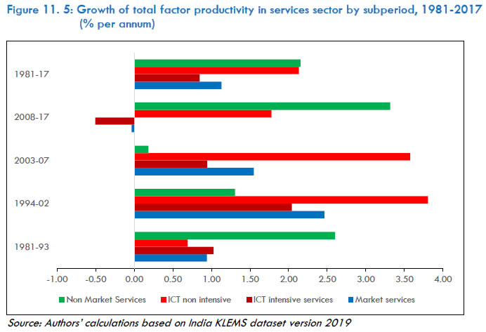 The TFP growth for broad categories of services is depicted in Figure 11.5. In the pre-reform phase of 1981-93, TFP growth of non-market services outperformed that of market services. However, we observe an improvement in the TFP growth of market services in the reform phase of 1994-02. It is clear that market services maintained this lead over non-market services in the golden growth phase of 2003-07 as well. However, TFP growth rate of market services fell considerably behind non-market services in the global slowdown phase of 2008-17. The low TFP growth of market services in relation to non-market services during the pre-reform phase and the global slowdown phase, leads to the overall picture with higher TFP growth of non-market services over market services for the entire period of 1981-2017. Within market services, we observe a peculiar trend—TFP growth of ICT intensive services consistently fell behind ICT non intensive services, after having outperformed the latter in the pre-reform phase. This trend is explored further below. Next, we look at the TFP growth performance for the individual sectors of services in Figure 11.6. For the entire period of 1981-2017, the subgroups with the highest TFP growth are public administration, transport and storage, and business services neck-and-neck with financial services. If we follow these industries through the four sub-periods, we find that public administration consistently registered high TFP growth rates for each sub-period before coming out on top in the global slowdown phase of 2008-17. In the case of transport and storage, it is interesting to note that the sector started off with a very low base TFP growth in 1981-93 before seeing improvements in its TFP growth in the post economic reform era, slowing down afterwards in the global slowdown phase of 2008-17. Both financial and business services registered decent TFP growth in the pre-reform phase, however in the mid-1990s, the sectors saw a great decline in TFP growth during 1994-2002—a period of Asian financial crisis and slowing down of the global economy. The post and telecommunications sub-sector presents another interesting case, the sector started off with a negative TFP growth (-0.86 percent per annum) in the pre-reform phase before seeing massive improvements in the sub-periods of 1994-02 and 2003-07, only to crumble down to an even worse negative growth rate (-2.23 percent per annum) once again in the global slowdown phase of 2008-17. The performance of other subgroups especially non-ICT and non-market services seem to broadly reflect the macro picture of the last figure. 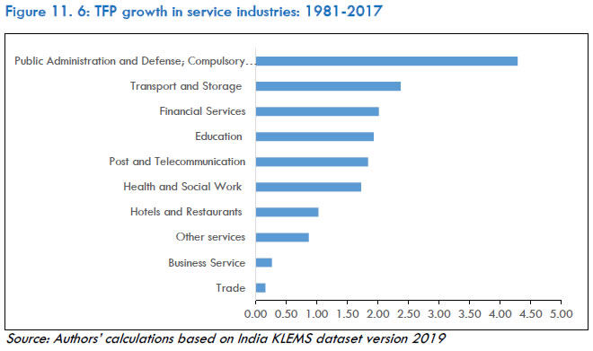 Figure 11.7 provides the TFP levels180 for services and its sub-sectors along with the disaggregated service industries for the period of 1981-2017. Panel A provides the TFP levels for overall services and its market and non-market sub-sectors. Since the reforms in 1991-92 we find that the TFP levels of the services sector has been improving and continues to be on an upward trajectory even after the Global Financial Crisis of 2007-08. The non-market services sub-sector has been leading the service sector TFP performance and continues to be higher than the overall services. Panel B provides the TFP levels for all disaggregated services industries for the period 1980-2017. Two points important to emphasise here are (1) the rise in services TFP levels across a majority of the industries began from the 2000s and most of these industries show rising trends during 2003-08, the period when India’s economic growth was growing around 8 per cent per annum, and (2) even during the phase of a global slowdown, TFP levels for India’s services industries continued to rise. An important aspect of the rising trends in TFP level for non-market services throughout the period of 1980-2017 is that the TFP level for public administration was increasing as early as the late 1990s. 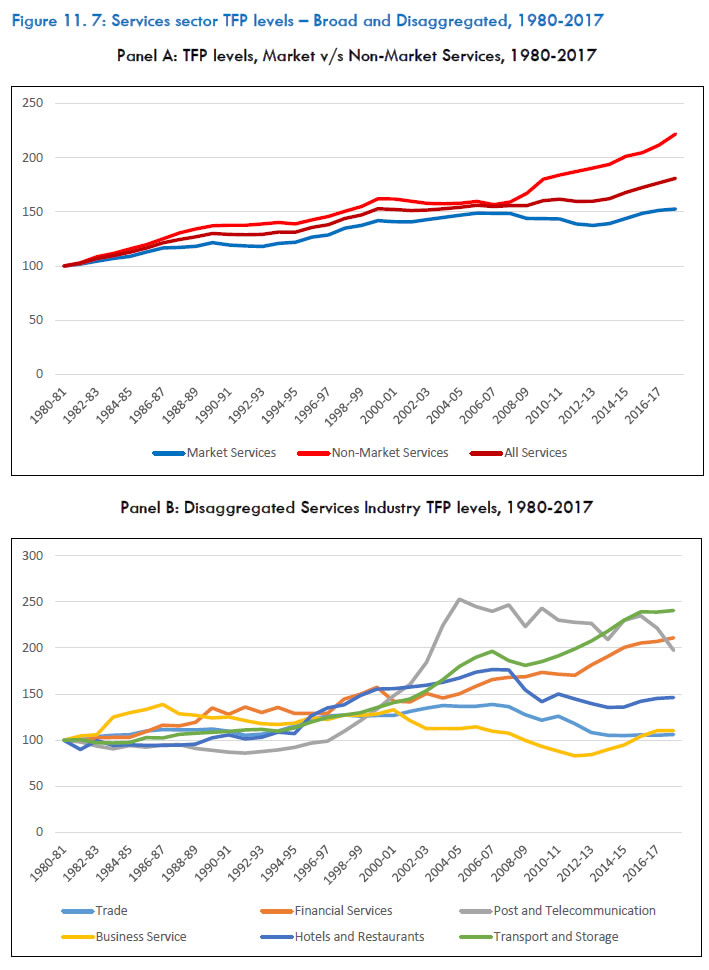
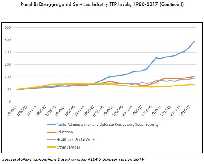 Table 11.5 presents the decomposition of output growth for the different sub-sectors of services for the period of 1981-2017. The contribution of an input is defined as the product of value share of the input and the growth rate of the input. Thus, each input contributes to output in proportion to its value share, while TFP contributes to output growth point for point. The first column reflects the rate of output growth, and the other columns reflect the contributions of the factor inputs — labour, capital, material, energy and services and the final column provides the rate of TFP growth. We observe wide variations in output growth across different service industries, from over 12 per cent p.a. growth in public administration (the highest) to 5 per cent p.a. growth for ‘other services’ (the lowest) for the period of 1981-2017. TFP growth comes out as the dominant source of output growth for public administration.181 When we compare the contribution of factor inputs, we find that capital services make the largest contribution to the output growth across different industries—trade, financial services, health, and business services182 and the rest of the services that make up for ‘other services’. Services input is observed to be the dominant source of output growth for transport and storage. We find material input as the dominant source of output growth for hotels and restaurants, and post and telecommunications. In the case of telecommunications, we have witnessed major deregulation since 1992 along with the onset of major liberalisation in manufacturing and trade sectors. Further, it may be important to note that telecom policy reforms have recognised the need to have many more participants than the incumbent operator in the process of telecommunications network expansion and service development, thereby bringing in competition which made the industry efficient in terms of TFP dynamics.183 It is evident from the decomposition of output growth that capital input, namely capital services, makes a significant contribution to the observed growth. In addition, for certain sectors namely health, education, financial services, trade including wholesale and retails, and hotels and restaurants, capital services account for a substantial contribution to improvements in labour productivity during the period 1981-2017, as seen before in Figure 10.4. This might indicate the role of increasing ICT in contributing to labour productivity growth. | Indian services are becoming highly intensive in capital on the one hand and on the other hand, the share of capital-intensive sub-sectors within the service sector is increasing. | Further, we note from Table 11.5 that for market-based ICT intensive sectors—financial services, business services and trade, capital service contribution is overwhelmingly large when compared with other inputs, thereby reflecting sharp inter-industry variations in the contribution of capital deepening within services. It would suggest that Indian services are becoming highly intensive in capital on the one hand and on the other hand, the share of capital-intensive sub-sectors within the service sector is increasing. | Table 11.5: Contribution of factor inputs and TFP to gross output growth, 1981-2017 (% per annum) | | Industry description | GO Growth | Contribution of Labour Input | Contribution of Capital Service | Contribution of Material Input | Contribution of Energy Input | Contribution of Service Input | TFPG | | Trade | 6.97 | 1.33 | 4.04 | 0.31 | 0.21 | 0.96 | 0.09 | | Hotels and Restaurants | 6.08 | 0.61 | 1.05 | 3.20 | 0.18 | 1.05 | 0.00 | | Transport and Storage | 7.08 | 1.10 | 0.80 | 1.14 | 1.49 | 1.80 | 0.66 | | Post and Telecommunication | 9.97 | 0.70 | 2.18 | 4.09 | 0.76 | 1.49 | 0.45 | | Financial Services | 8.72 | 1.63 | 2.97 | 0.44 | 0.22 | 1.64 | 1.44 | | Business Service | 12.40 | 2.34 | 4.94 | 1.63 | 0.40 | 3.35 | -0.47 | | Public Administration and Defence; Compulsory Social Security | 5.94 | 0.33 | 0.82 | 0.31 | 0.02 | 1.33 | 3.07 | | Education | 7.86 | 2.56 | 2.32 | 0.24 | 0.03 | 1.05 | 1.49 | | Health and Social Work | 6.62 | 1.50 | 1.98 | 2.07 | 0.03 | 0.29 | 0.57 | | Other services | 5.56 | 1.63 | 1.90 | 0.59 | 0.02 | 0.63 | 0.61 | | Source: Authors’ calculations based on India KLEMS dataset version 2019 | The share of ICT intensive sectors (trade, post and telecommunication, financial services) within market services stands at almost 40 per cent of total services (2009-10). This may be due to several reasons, including import of capital goods following liberalisation of trade policy, especially lowering of tariffs and easing of nontariff barriers in the capital goods sector.184 It may also reflect the onset of many new technologies (ICT) that enhances capital deepening through liberalisation of trade in services. Table 10.6 captures changes in trade policy—nominal tariffs as well as resultant import competition brought about by such changes. Das (2015)185 finds that for all categories of capital goods, there has been substantial downward shifts in nominal tariff rates as captured by nominal rate of protection. We find across-the-board decline in tariff rates from around 50 per cent to almost below 20 per cent during the decades of 1990s and 2000s. We find that for office and other computing machineries there is a substantial decline of more than 50 percentage points. | Table 11.6: Trade policy indicators for capital goods sector: 1990s versus 2000s | | | Industry Description | Import Penetration Ratio | Nominal Rate of Protection (%) | | | Capital Goods Industries | 1990-1999 | 2000-2009 | 1990-1999 | 2000-2009 | | 350 | Agri machinery and equipment and parts thereof | 0.01 | 0.03 | 44.76 | 18.10 | | 351 | construction and mining industries | 0.71 | 1.24 | 44.39 | 17.45 | | 352 | Prime movers, boilers, steam generating plants nuclear reactors | 0.42 | 0.92 | 44.39 | 17.45 | | 353 | Industrial machinery for food and textile industry | 0.41 | 0.82 | 45.10 | 17.76 | | 354 | Industrial machinery other than food and textile | 0.56 | 1.12 | 44.39 | 17.45 | | 356 | General purpose Machinery | 0.61 | 1.24 | 50.54 | 17.98 | | 357 | Machine tools parts and accessories | 0.09 | 0.27 | 46.51 | 17.39 | | 358 | Office, computing and accounting machinery and parts | 1.16 | 1.05 | 62.73 | 12.37 | | 359 | Special purpose machinery and equipment/component/accessories | 0.93 | 1.45 | 50.54 | 17.98 | | 360 | Electrical industrial machinery | 0.07 | 0.17 | 48.87 | 17.72 | | 361 | Insulated wires and cables | 0.02 | 0.09 | 71.80 | 19.45 | | 362 | Primary cells and primary batteries | 0.03 | 0.12 | 79.63 | 21.02 | | 365+366 | Radio and TV apparatus | 0.20 | 0.43 | 63.38 | 12.78 | | 368 | Electronic valves and tubes | 0.71 | 0.75 | 63.38 | 12.78 | | 369 | X-ray Machines and Electrical equipment nec. | 1.18 | 0.97 | 63.38 | 12.78 | | 370 | Ship and boat building | 0.31 | 0.89 | 52.19 | 18.93 | | 371 | Locomotives and parts | 0.15 | 0.42 | 46.88 | 18.15 | | 372 | Railway/tramway wagons and coaches | 0.05 | 0.12 | 46.88 | 18.15 | | 379 | Transport equipment and parts | 0.01 | 0.01 | 72.46 | 21.27 | | Source: Das D K (2015): Trade Liberalization Indicators by Industry—India DATABASE— unpublished | The observed growth pattern in the service sector has not been uniform across all services in India. The performance of market-based ICT intensive sectors is impressive, especially telecommunications and financial services. However, by and large, we find dominance of capital deepening in accounting for growth. We need to ascertain if information and communication technology (ICT) remained an important source of both capital deepening and total factor productivity growth within services in India. We conclude that import liberalisation has been a principal component of the economic reforms undertaken in India and complementary policies such as technology import policy have, to a large extent, contributed to the import and adaptation of ICT equipment and technology in the observed capital deepening within services. Services and Aggregate TFP The trajectory of growth in TFP is a key determinant of long-run economic growth of an economy. Further, the service-led growth momentum in India has been questioned on the grounds of ‘sustainability’ against the backdrop labour-abundance and capital-scarcity. To this end, we examine the contribution of different sectors to productivity growth at the aggregate economy level. The decomposition of output growth into its sources is shown for all broad sectors of the economy. The whole period 1980-2017 is considered for the analysis. The contributions of different inputs to output growth are shown in Table 11.7. TFP has played an important role in the growth of the services sector. TFP growth accounted for about a fourth of the real GVA growth achieved by the services sector. Besides productivity growth, labour and capital input growth also contributed to services sector growth while capital input growth emerged as relatively more important. | Table 11.7: Contribution of factor inputs and TFP to GVA growth by broad sectors: 1981 to 2017 (% per annum) | | BROAD SECTOR | Real value- added growth | Contribution of Labour persons | Contribution of Labour quality | Contribution of Capital services | TFP growth | | Agriculture | 3.06 | -0.0017 | 0.17 | 1.79 | 1.10 | | Mining and Quarrying | 5.02 | 0.30 | 0.39 | 5.43 | -1.10 | | Manufacturing | 6.84 | 0.71 | 0.25 | 5.80 | 0.07 | | Electricity, Gas and Water Supply | 6.76 | 0.89 | 0.21 | 4.46 | 1.21 | | Construction | 5.90 | 4.77 | 0.31 | 2.23 | -1.42 | | Services | 7.31 | 1.69 | 0.34 | 3.67 | 1.61 | | Total economy | 6.03 | 1.28 | 0.27 | 3.60 | 0.87 | | Source: Authors’ calculations based on India KLEMS dataset version 2019 | The aggregate TFP growth is impacted by the vast heterogeneity that exists across industries in the form of a few subgroups dominating the growth of output and productivity over extended periods of time. This can often result in a distorted scenario, as the role of the leading industries can dramatically shift the TFP scenario observed over a period of time. Figure 11.8 depicts industry-wise contribution to aggregate TFP growth for the period 1981 to 2017. The top three contributors include agriculture, hunting, forestry and fishing, public administration and defence, and transport and storage. Financial services and the services that make up for ‘other services’ were significant contributors as well. This substantiates our assertion about the growing importance of services in the overall economy and, to a considerable extent, it also evident that high productivity growth in many service sectors underlies the current dynamism in service sector growth. 11.5. Conclusions Service sector in India also grew rapidly in the third subperiod (2003-11) and its growth was, in fact, higher than the growth in agriculture and manufacturing. It remains to be seen, however, whether growth in services will lead to inclusive overall growth in India. This chapter is an attempt to understand India’s service sector productivity growth dynamics observed since the 1980s. We examine productivity trends in the service sector at disaggregated industry level using carefully developed India KLEMS panel data for the period 1981-2017. We use both the VA as well as GVO frameworks in computing labour and total factor productivity growth based on growth accounting technique. In addition, a decomposition exercise was done to account for (1) sources of labour productivity growth and (2) sources of output growth. Our findings suggest the following: Labour productivity in India’s service sector has been growing substantially over the decades, and much of this productivity gain is accruing through acceleration in market services-based industries. This observed productivity gain in the market services, particularly ICT-intensive services, might indicate the role of increasing ICT in contributing to labour productivity growth. The labour reallocation effect is positive in all the sub-periods, and has increased in the 2000s, suggesting a structural transformation that is growth enhancing. Our TFP estimates based on KLEMS production function for the services sector indicate impressive growth in TFP for market-based services. The nonmarket-based services, on the other hand, indicate a progressive decline in resource use efficiency in the recent decades. It is evident from the decomposition of output growth that capital input makes a significant contribution to the observed growth. This indicates a dominance of capital deepening in accounting for growth. We need to ascertain if information and communication technology (ICT) remained an important source of both capital deepening and total factor productivity growth within services in India. We infer that import liberalisation has been a principal component of the economic reforms undertaken in India, and along with complementary policies such as technology import policy, have largely contributed to the import and adaptation of ICT equipment and technology in the observed capital deepening in the services industries. Finally, the growth and productivity performance of services highlighted in this chapter points to several issues that need attention in the form of future research endeavours. It would also be useful to undertake international comparison of services in emerging economies like India. This will require internationally comparative datasets for meaningful comparisons. For India, this challenge has been resolved to a large extent by the India KLEMS dataset, which follows the EU KLEMS classification. However, problems remain with several other aspects of data pertaining to the service sector. | It is evident from the decomposition of output growth that capital input makes a significant contribution to the observed growth. This indicates a dominance of capital deepening in accounting for growth. | Nayyar (2012) has raised several concerns about the service sector data base and the present study addresses several of these. First, the methods for measuring service sector output have been considerably improved, although concerns persist regarding measurement of market services output. A study by Timmer et al. (2010) analyses the issues regarding measurement of output for different categories of market services and regarding price deflators for each of the service industries in general. Second, we address the significant need for an appropriately constructed variable to measure capital input for the service sector. Our construction of the capital services variable that our study used in estimating total factor productivity is the first such estimate of capital input for the Indian economy at an industry level and covers all the 10 subgroups of services. Third, recognising the importance of individual segments of service sector, this study addresses the issues of sources of growth at both the broad segments of services—market versus nonmarket services or ICT-intensive services versus non-ICT intensive services and for different industries within the service sector. For further research, there are several questions that need to be addressed—the need for more data that could cover other aspects such as rural-urban decomposition of service industries to understand where the dynamism lies; and the need for more field surveys to understand the occupational structure of informal sector—hawkers, transport drivers, and even domestic workers. Finally, it is also very important to understand the drivers of growth in services in two emerging markets—China and India. As a part of this future research agenda, we intend to follow up on the present study with a comparative analysis of service industries in India and China using the KLEMS dataset for each country. We end with the quote, “If the data is so dodgy, should all analysis on the services sector be called off? As is evident, this would mean the entire economy, since services account for more than a half of GDP. Conversely, should economists be like the drunk who looks for a lost key under the lamp-post because that is the only place where there is light? Given the need for analysis, there can be only one answer.” (Jain and Ninan, 2010). Annexure 11A: Policies Relating to Services Sector | Table 11A.1: Selected policies of services in India—A schematic view | | Issues | Policies | | FDI | - Allowing 100 percent retail trade
- Raising FDI cap in Insurance sector ( from 26 per cent) and in Banking ( allowed 74 percent FDI+FII)
- 100 percent FDI allowed in Construction
- FDI open for entertainment sector- news and current affairs TV channel
- FDI in air transport services
- FDI for modernization of railways | | Disinvestment | − Disinvestment of public sector units both within central and state governments | | Tariff and Tax | specific sector issues
− Shipping services (tonnage tax issues, zero rating input services, seafarer taxation issues, customs duty/excise duty exemptions, withholding tax)
− Tourism services) rationalizing tax structure, ATF taxation, state luxury tax, per seat passenger tax, fees for monuments and tax payment modes)
− Entertainment Services (tax credit issues)
− Health care services (zero tariff for medical equipments; exemptions at state level for capital goods used in hospitals)
− Telecommunications (customs bonding, taxability of items between federal and state governments; service tax on IT software)
− Air transport services (sales tax issues, import duty of spare parts, turnover tax by airports)
− engineering services (customs and excise duties, stamp duties)
Other related issues
Clarity on service tax refund policy on input services used
− Transfer pricing issues
− Single return for service tax and excise tax
− Reduction of tax deducted at source | | Credit and Finance | − Withholding tax on interest paid on ECB
− Issues connected with venture capital funding
− Extending dedicated lines of credit | | General issues | − Showcasing India’s services overseas
− Measures for promoting service exports
− Standardization of services
− Consolidation of service providers in each category
− Service portal
− Preferential system for overseas investor and government | | Source: Authors’ compilation from Prasad and Sathish (2010). |
Chapter 12: Growth and Productivity: A China and India comparison186 12.1 Introduction The growth stories of India and China, the two most populous countries with substantial political and institutional differences, have received wide attention in recent economic literature (Nayyar, 2019; Wu et al, 2016; McMillan and Rodrik, 2013; de Vries et al, 2012; Bosworth and Collins, 2008; Lee, Rao, and Shepherd, 2007; Bardhan, 2006; Prasad and Rajan, 2005; Hulten and Srinivasan, 1999). Since the initiation of pro-market reforms in India in 1991 and the revival of Chinese reforms and opening-up programme after Deng Xiaoping's southern China tour in 1992 following the 1989 Tiananmen Square protests, the global presence and impact of these two giant economies have increased. The Soviet-type planned economy approach at the centre of early-stage economic policymaking in both India and China accorded a significant role to the government and largely undermined the role of the market and private sector in driving economic growth. However, the degree of freedom for the private sector to operate differed substantially between the two economies, with China being extremely restrictive. India started a partial liberalisation initiative in the mid-1980s, often considered as pro-business reforms that supported the already-established industrial and commercial establishments, yet with a limited role of market forces (Rodrik, and Subramanian, 2005). Amid a significant balance of payment crisis in the early 1990s, India introduced more stringent market reforms abolishing its licensing system and opening the economy to foreign investment. China, too, started full-fledged pro-market reforms in the 1990s. However, with its authoritative regime, China implemented a massive manufacturing programme and invested heavily in manufacturing infrastructure, which created an export-oriented manufacturing-driven growth path for the country. Although India also devised several policies to develop its manufacturing sector, the country’s growth success was primarily in the services sector. With its significant pool of skilled and educated labour force, it has seen faster growth in several market services, notably computer and software-related services. China's joining of the World Trade Organisation (WTO) at the end of 2001 further helped expand its manufacturing, and resulted in its economy growing at an unmatched speed. Thus, both countries had a distinct path of economic growth, as the sectoral pattern in driving aggregate growth differed substantially. Yet, the two economies have performed far better than the rest of the emerging world. According to the Conference Board's Total Economy Database187, the Indian economy grew at an annual average rate of 6.9 per cent during 1992-2018 and China's official growth rate was 10 per cent for the same period. The official GDP estimates of China, however, is highly contested (see Wu, 2013 and 2014a). Alternative estimates of Chinese GDP by the Conference Board following Maddison and Wu (2008) suggest an annual average growth of 7.3 per cent during this period. Obviously, India and China's fast GDP growth also helped improve their standards of living. Their per capita incomes increased at an average annual rate of 6.6 per cent (China) and 5.2 per cent (India) during 1992-2018, reducing the income gap with the global frontiers. As of 2018, the average Indian's income, evaluated in purchasing power parity terms, is close to 11 per cent of the average American's income, compared with 4.5 per cent in 1992. For China, the relative per capita income is nearly double that of India, as it increased from 6.4 per cent of the US level in 1992 to 20.5 per cent in 2018. Previous literature has investigated the sources of growth in India and China, both in country-specific studies and in a comparative perspective (Bosworth and Collins, 2008; Lee, Rao, and Shepherd, 2007; Prasad and Rajan, 2005; Nagraj, 2005; Hulten and Srinivasan, 1999; de Vries et al, 2012; McMillan and Rodrik, 2011; Wu et al, 2016). These studies generally suggest a positive role of market-oriented reforms in triggering productivity growth, which played a significant role in China and India's growth stories. Past studies comparing the two economies mostly used aggregate or broad sector data to examine sources of growth —considering the importance of proximate sources, factor accumulation, and total factor productivity (TFP)—in both countries (see for e.g., Bosworth and Collins, 2008), which undermines the importance of sectoral reallocation of resources and the differences in factor price across sectors.188 For instance, using microdata on manufacturing firms, Hsieh and Klenow (2009) suggest substantial misallocation of labour and capital across sectors which has distorting effects on aggregate manufacturing productivity. Given that the two economies followed substantially different growth paths, the growth stories derived using aggregate data may conceal several industry dynamics. This is particularly important for productivity comparisons, as technological developments typically happen at the industry level. This chapter considers the inter-industry differences in productivity for examining the growth dynamics in India and China. Such industry level analysis of sources of growth requires a significant amount of detailed data in a comparable setting for both countries in a consistent national accounts framework. The KLEMS initiative facilitates the availability of such data, and we utilise the China KLEMS data along with the India KLEMS data in this chapter. | As China and India followed substantially different paths, studies of their growth stories that are derived using aggregate data, conceal varying industry dynamics. This chapter considers the inter-industry differences in productivity, which requires comparable detailed data of the kind KLEMS provides. | The chapter is organised in five sections. In the second section, 12.2, we provide an overview of relative levels of labour productivity in India and China compared with select developing economies and examine the trends in aggregate labour productivity growth rates in the two economies. Section 12.3 discusses the aggregation of industry output and productivity growth rates into broad industrial groups used in the study. This section also discusses the China KLEMS data and its comparability with India KLEMS data, discussed in Chapter 2. Section 12.4 starts with a discussion of the results of labour productivity and TFP growth comparisons at the broad sectors of the economy for four time periods, 1980-1992, 1993-2002, 2002-07 and 2008-17. We then discuss the results for the nine industry groups based on the final use of the industry output and distinguishing between market and non-market economies. The last part of this section provides an econometric analysis of the impact of capital deepening on labour productivity growth to compare the differences in the effectiveness of capital intensification between India and China. The section also compares the industry pattern of aggregate TFP growth, using detailed industry data for the two economies. Section 12.5 concludes the chapter. 12.2 Labour Productivity and growth in India and China: The aggregate picture Before delving into the analysis of detailed industry-level data, we look into the general trend in India and China's aggregate economy labour productivity levels from a comparative perspective. Figure 12.1 shows the relative levels of labour productivity in the two economies compared to a few select emerging market economies. The labour productivity levels in this chart are expressed as a percentage of the level in United States. A few points warrant attention. First, both India and China are still far below the US productivity levels—China at 17.5 per cent of the US level, and India at 13.7 per cent.189 Second, both these countries have substantially improved their relative productivity performance since 1992, i.e., during their post-market reforms era—they were at 5 per cent of the US level in 1992. Third, the productivity levels in the two economies are still the lowest compared with other emerging market peers, such as Russia, South Africa, Brazil (the BRICS), and some Asian economies such as Malaysia and Indonesia. Fourth, a noticeable difference compared with other BRICS countries is that while Russia, Brazil, and South Africa have seen an erosion in their productivity levels, India and China have continued to climb up the productivity ladder. All this indicates the relatively faster pace of productivity expansion in China and India compared with other emerging market economies, and potential for further improvement. | While productivity levels in India and China are the lowest compared with other emerging market peers and some Asian economies, both are improving productivity at a relatively faster pace and show potential for further increase. | The two economies started from a very low base in labour productivity in the pre-reform years, with India growing at a mere 2 per cent and China at close to 4 per cent in the 1980-92 period (Figure 12.2) and their labour productivity levels being at about 5 per cent of the US levels in 1992 (Figure 12.1).190 China experienced rapid growth in productivity in the 1990s, far more than India. During the 1994-2002 period, China's aggregate labour productivity growth was as high as 6 per cent compared with only 3 per cent in India. China subsequently maintained its 6 per cent aggregate productivity growth during the 2000s, while India, despite growing a bit, remained below 5 per cent—lower than China— China's faster growth created a gap between India and China in terms of productivity levels, as Figure 12.2 shows that between 1980 and 2017, China's productivity index grew seven times, but less than four times in India. 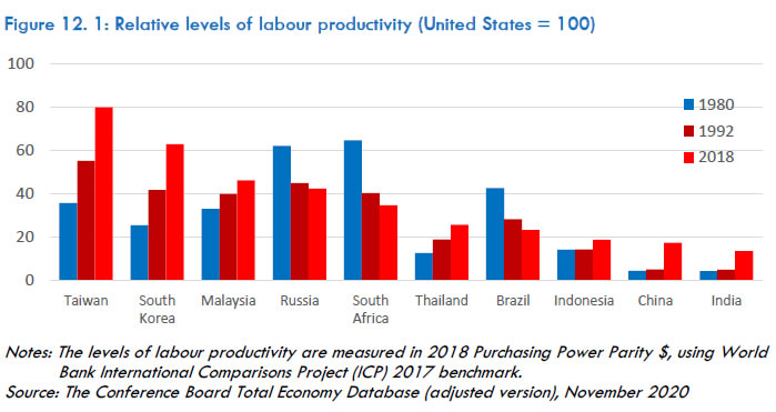 Two important questions regarding the sources of productivity growth are first, whether this divergence in productivity growth between the two economies is a phenomenon across the board or whether it emanates from a few industries and second, whether the labour productivity growth in these economies is driven by factor accumulation or total factor productivity. We examine this by comparing labour productivity growth rates and its proximate sources—capital deepening and total factor productivity growth—among various sectors of the economy. 12.3 Aggregations of KLEMS industry growth rates: Methodology and data 12.3.1 Methodology Productivity growth of India and China will be compared using the standard growth accounting method explained in Chapter 2 of this report. The India KLEMS database provides detailed data on inputs and output for 27 industries (see Chapter 2 for a discussion of India KLEMS data). The China Industry Productivity Database, or CIP/China KLMES provides data for 37 industries. However, to facilitate a meaningful comparison, we aggregate the 27 India KLEMS industries and 37 China KLEMS industries into industry groups, as in Erumban et al. (2019a) (see Table 12A.1 in Annexure). These aggregations are performed using simple value-added weights, which account for industry heterogeneities in output price differences. These weights are applied to industry growth accounting results, obtained using value added function as in equation (7.6), i.e., 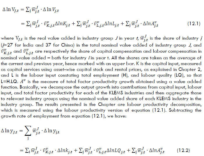 where y is labour productivity, measured as value added per worker (y=V/H) and k is capital deepening measured as capital services per worker (k=K/H). Given that the more appropriate measure of output at the industry level is gross output rather than value added, one could alternatively use a direct aggregation procedure suggested by Jorgenson et al. (2007). In this approach, one would decompose the growth rate of industry output rather than industry value added, and therefore, the weights of TFP in equation 12.1 and 12.2 would be the well-known Domar weights — the ratio of industry gross output to the aggregate value added. In such an approach, it is also possible to calculate the reallocation of capital and labour to sectors with better returns to these inputs (see Jorgenson et al., 2007; Erumban et al., 2019a; Wu et al, 2016, and Chapter 7 of this report).191 12.3.2 CIP/China KLEMS Data Recall that the practical implementation of the growth accounting methodology requires data on value-added, employment, labour quality, capital services and labour and capital income shares to decompose the growth rate of value added or labour productivity (value added per worker) into contributions from factor inputs (employment, labour quality and capital services) and the residual total factor productivity growth (see Chapter 2). All the relevant data for India on value added, employment, labour quality, capital services and labour income share are obtained for 27 industries from India KLEMS (See Chapter 2). For China a comparable dataset for 37 industries is obtained from China Industry Productivity Database (Wu, 2020).192 We use the updated and revised version of the CIP data based on the publicly available CIP 3.0 as discussed in Wu (2020) (see Wu 2015; Wu and Ito 2015; Wu, Yue, and Zhang 2015 for the details of data construction, data sources and problems). In what follows, we discuss the construction of variables relevant to this chapter in the China KLEMS. Output and value added: The CIP industry accounts for output, value added, and intermediate inputs are made coherently consistent with the Chinese national accounts, and therefore, any bias in Chinese official data (see Wu 2013, 2014a, 2014b) will prevail in the industry database (Wu and Ito 2015). The nominal accounts of output and value added are deflated by industry-level producer price index (PPI), constructed using official PPIs for the agricultural and industrial sectors and consumer price index (CPI) or its components for service industries (Wu and Ito 2015). All the data used in this study are based on a single deflation approach assuming changes in input prices are the same as changes in output prices, which is similar to the Chinese national accounts practice. Earlier, we indicated that there had been significant debate about the reliability of China's official GDP estimates, and therefore, alternative GDP measures have been developed. However, such alternative measures were nearly impossible to construct at the detailed industry level, and therefore, the industry data used in this analysis are consistent with the official data. | Data on value added, employment, labour quality, capital services and labour income share for 27 industries are from India KLEMS. For China a comparable dataset for 37 industries is from China Industry Productivity (CIP) Database | Employment and labour quality: The employment data in the CIP industry accounts are built on all available employment statistics and surveys, reconstructed to ensure consistency with available population censuses. Total employment, which includes self-employed workers, is cross classified by gender, age, and educational level based on information from the census and surveys. These different types of labour are weighted by their compensation shares at the industry level to construct labour quality measures, as described in Chapter 2 (Wu, Yue, and Zhang 2015). Capital stock and capital services: Annual investment flows by industry are constructed for the industrial sectors using official gross fixed assets data at historical costs. For non-industrial sectors, an official investment series is adopted. The final series is reconciled with the national accounts gross fixed capital formation data for the aggregate economy. The capital stock by industry is estimated using the perpetual inventory method (see Chapter 2), for which the initial capital stock for each industry and asset is estimated by China's first asset census in the early 1950s (Wu 2015). Industry-specific investment deflators are constructed using PPIs of investment goods industries and the nominal wage index of construction workers (Wu and Xu 2002; Wu 2008 and 2015). Similarly, industry-specific depreciation rates are estimated based on asset service lives and declining balance values used in the US national accounts that follow the approach developed by Hulten and Wykoff (1981). The total investment is divided into two asset types - construction and equipment, and aggregate capital services are estimated using capital stock estimates for these two assets, along with rental prices of assets, the measurement of which is described in Chapter 2. Compatibility of the Indian and the Chinese Data Both the Indian and the Chinese data follow the KLEMS principles in measuring primary inputs and output accounts, and therefore their methodologies are quite comparable. Construction of each variable at the industry level is in principle ensured to maintain coherence in the national aggregates, although it is always challenging to deal with missing data and data quality problems. It is impossible to assess how the remaining data problems may have affected our estimates. However, it is reasonable to argue that these problems are limited. One important point to be noted, however, is that all volume indicators in the Chinese data are measured in 2000 prices, but in 2011-12 prices for India. Moreover, India's data are measured for the financial year, running from April 1 to March 31, whereas China's data is the calendar year. | Both the Indian and Chinese data follow the KLEMS principles in measuring primary inputs and output accounts, making their methodologies quite comparable. Construction of each variable at the industry level is in principle ensured to maintain coherence in the national aggregates. | The next issue is the estimation of the capital stock. The Indian data includes three capital assets, namely machinery, transport equipment, and structures, whereas the Chinese data set provides only two assets, that is, machinery mixed with transport equipment and structures. This might have implications for the measured TFP growth (TFPG) rates, as the depreciation rates and rental prices of transport equipment would differ from that of machinery. Therefore, it may affect the measured capital service growth rates and, therefore, TFP. However, we do not expect the problem to be substantial. Finally, due to lack of information, especially for India, we use the number of employed persons as a measure of labour input rather than hours worked. This means that we implicitly assume that an average worker's hour intensity is constant over time, across industries, and between the two economies. As shown in Wu, Yue, and Zhang (2015), however, in China's case, the hour intensity rose substantially from the early 1990s through post-WTO heydays of rapid export-oriented growth and then dropped in the wake of the global financial crisis. 12.4 Empirical results 12.4.1 Labour productivity and TFP in the broad sectors of the economy We decompose labour productivity growth in each of the 27 industries in India and 37 industries in China into contributions from capital deepening, labour quality, and TFP, using the standard growth accounting approach. Subsequently, these industry growth rates are aggregated using value-added weights as explained in equation (12.2) to useful industry groupings. In this section, we first document the trends in Tonrquvist aggregated labour productivity and total factor productivity growth rates in the three broad sectors of the economy —agriculture, industry (manufacturing, mining, utilities, and construction), and services (market and non-market) sectors. We subsequently compare the productivity trends in the two countries for nine industry groups (Tonrquivst aggregates)—agriculture, other goods production, consumer and intermediate goods manufacturing, investment goods manufacturing, trade and distribution, other market services, financial services, business services, and non-market services. The dataset used in this study covers the period 1980-2017, and all analyses are made for three time periods—1980-92, 1993-2002, 2003-17. This periodisation is chosen in line with the other chapters in this report and is consistent with major policy changes in both economies. The period 1980-92 was that of early reforms in both countries—China's agricultural and industrial reforms, and India's first set of pro-business reforms. The second period, 1992-2002, coincides with China's market reforms after the Tiananmen square unrest and India's complete overhaul of economic policy towards a pro-market economy. The last period, comprising the years after 2002, is the post-WTO period for China and was also a period of high growth in India. We further sub-divide the last period into pre-, and post-global financial crisis, i.e., 2002-07 and 2008-17. | We decompose labour productivity growth in India’s 27 industries and China’s 37 industries into contributions from capital deepening, labour quality, and TFP. We then aggregate these industry growth rates using value-added weights into useful industry groupings. |
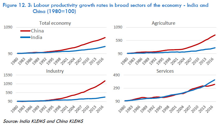 Figures 12.3 and 12.4 depict the growth trends in labour productivity and total factor productivity at the broad sector level in India and China. The top-left chart in Figure 12.3 is the same as Figure 12.1 but is reproduced here to get a perspective compared with sectoral patterns of growth. The difference in the aggregate labour productivity growth between China and India is primarily a reflection of the differences in agricultural and industrial sectors. In these sectors, China has made a massive stride in productivity growth compared with India. Productivity in China's agricultural sector improved by seven times during the last four decades, but only by four times in India. In the industrial sector, the gap was even bigger, as the Chinese economy improved its productivity by nearly 13 times, compared with just three times higher productivity in India over the same period. Expansion in the service sector, was however, more comparable for both countries. In fact, India did better than China, with four times higher productivity compared to three and half times higher in China. 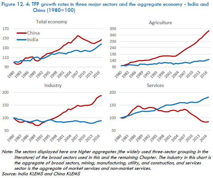 In Figure 12.4, the trends in TFP growth between the two countries suggest a slightly different picture. China performed well in terms of TFP in the aggregate economy, agriculture, and industry, but in the service sector its performance was much worse than India’s. The early upward trend in China's TFP came to a halt around 1989—the year in which China faced a severe political crisis. Although the period was characterised by China’s agricultural and industrial reforms, the industrial sector did not see any productivity gain in the pre-1989 years. While TFP in both agricultural and service sectors improved, TFP in the industrial sector declined. Industrial TFP revived during the 1990s reforms, and continued to accelerate until the global financial crisis in the mid-2000s. Joining the WTO in 2001opened more avenues for Chinese manufacturing firms to benefit from the international market and improve their productivity growth during this period. While TFP in the agricultural sector continued to improve in the 1990s, the pace of the improvement escalated only after China joined the WTO. In contrast, TFP in the services sector, which currently accounts for more than half the Chinese GDP, has not improved since the late 1980s. Overall, the aggregate TFP improvement in the post-1990 period was driven by industrial and agricultural sectors, while its pace was moderated substantially by falling TFP in the services sector. Aggregate TFP had a retreat amid the global financial crisis, primarily driven by rapid erosion in the services sector's productivity and stagnation in industrial TFP growth. The Chinese services sector has seen a steep fall in productivity growth in the post-crisis period. Along with the continued rise in its labour productivity, this suggests the growing role of factor accumulation in driving services growth in the economy. 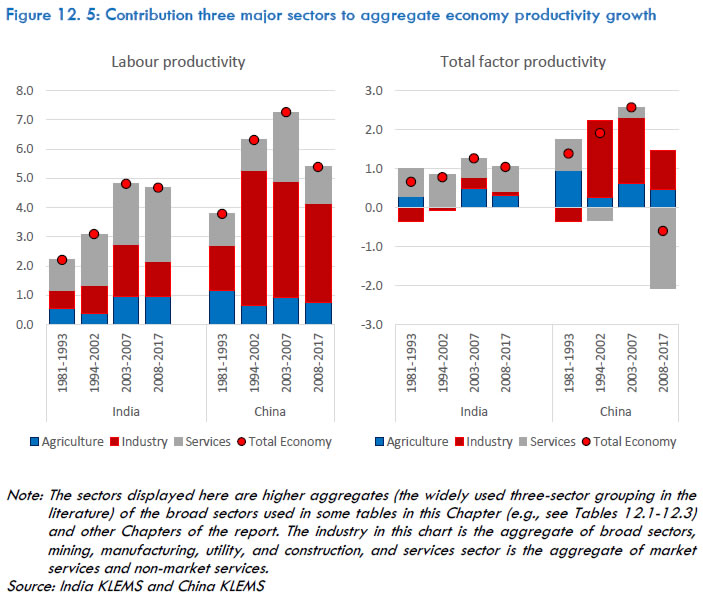 The aggregate economy TFP growth (TFPG) in India was not as impressive as that of China. That does not, however, dismiss the positive role that the reforms played in driving productivity growth. Unlike in China, where TFPG in the aggregate economy fell since the financial crisis, it has been rising consistently, albeit at a relatively slower pace. Since China's entry to the WTO, with its manufacturing boost, India’s rate of TFP growth has lagged substantially behind. Meanwhile, India’s continued acceleration in TFP even after the global financial crisis maintained its TFP close to China’s in recent years. However, a significant difference is that almost all of India's TFP growth came from the services sector (Figure 12.5). Indeed, the role of factor accumulation in India's services sector, which registered a comparable labour productivity growth as in China, was relatively smaller. India’s industrial sector TFP remained relatively weak. Although TFP growth improved over the years in the Indian agricultural sector, the pace was much slower than in China. Most of the labour productivity gains in China in the 1990s and 2000s were driven by its vibrant industrial sector, and almost all of its TFP growth in the 1994-2002 period and 70 per cent of TFP growth in the pre-crisis years after 2002 also came from the same sector. China’s service sector faced a significant productivity set back since the 1990s—except for a moderate uptick in the 2003-07 period, its contribution to aggregate TFP growth was negative, and its TFP deceleration was even more pronounced in the post-crisis period. Undeniably, economic reforms, opening up to the global economy, and global trade have helped both economies improve their productivity and competitiveness. Although the benefit of reforms did not accrue across the board, rather confined to agricultural and industrial sectors in China and to the service sector in India, the reforms did deliver a positive impact on productivity growth. While there has been a revival in India's service sector productivity in the post-crisis period, China has experienced a major setback in productivity in both the industry and services sector, with the latter facing massive deceleration. 12.4.2 Labour productivity and TFP in the select industry groups of the economy Although the KLEMS data covers 27 industries for India and 37 industries for China, to make a comparison between the two economies easier, we aggregate these industries into industry groups based on their product/service characteristics. In addition to user groupings, we also distinguish between market and non-market economy, where the non-market economy primarily consists of the education, health, and government sectors. This section discusses the results of this aggregation. In the left panel of Figure 12.6, labour productivity growth in India’s aggregate economy and its nine broad sectors has been decomposed into contributions from capital deepening (capital services per worker), labour quality, and TFP for the entire period of 1981-2017. There is substantial cross-industry variation in labour productivity growth. For instance, the industry group called ‘other market services’, including post and telecom services and hotels and restaurant services, had the highest annual labour productivity growth, at 5.1 per cent. The consumer and investment goods manufacturing sectors followed with 4.7 and 3.9 per cent productivity growth respectively. All other services, trade and distribution, finance, and non-market services except business services recorded annual labour productivity growth higher than 3.5 per cent. The weakest productivity growth was observed in the industry group ‘other goods production (mining, utility, and construction)’ at 1.8 per cent. It is worth examining which of the proximate sources explain the labour productivity growth—capital deepening, labour quality, or total factor productivity. Close to 70 per cent of India’s labour productivity growth in the aggregate economy came from capital deepening. The dominance of capital deepening was prevalent in most sectors, in the range of 60 to 95 per cent of labour productivity growth across industry groups. A few exceptions are non-market services and financial services (35-40 per cent) and other goods production group, where capital deepening was the sole source of labour productivity growth. The consumer goods manufacturing sector experienced the maximum capital deepening and in non-market services it was the least. 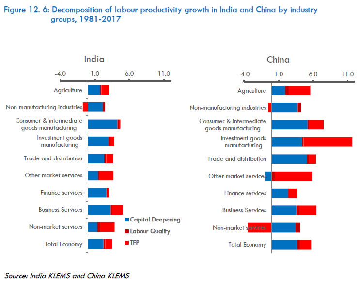 Non-market services, which include education, health, and government, are sectors with a high relative human capital contribution, in contrast to agriculture and financial services. Improvement in labour quality contributed less than 10 per cent of the economy's labour productivity growth, again with varying degrees across industry groups. In terms of the most interesting variable—TFP, non-market services performed relatively better, followed by financial services—both registered a 2 per cent annual TFP growth rate. Another sector with high TFP was the ‘other market services’ group, which includes telecommunications. The weakest TFP growth was in the ‘other goods production’ group and in consumer goods manufacturing. The former group with its negative TFPG, is a likely candidate for poor productivity growth as it includes electricity, gas, and construction. In India, the construction sector has been performing poorly in productivity, as much of the workforce released from agriculture ends up in the less skill-demanding construction sector, barely adding to its productivity (Erumban et al., 2019a). In general, manufacturing TFPG has been relatively weaker than the services sectors. In the aggregate economy, one-fourth of the labour productivity growth was due to TFP, with financial services dominating at more than half, and agriculture and other market services close to a third. Overall, the contribution of TFPG to productivity growth in the service sectors ranged from 20 to 50 per cent, while it was quite weak in the manufacturing sector—ranging from 1 per cent in consumer goods to 15 per cent in investment goods manufacturing. The picture changes drastically when looking at China (right panel of Figure 12.6). The highest labour productivity growth was in the manufacturing sector; investment goods and consumer goods registered labour productivity growth of 11.7 and 7.6 per cent respectively. Agriculture and the two market services industry groups also performed well with productivity growth ranging between 5.5 and 6.5 per cent. Other market economy sectors, financial services, and business services, and even the other goods-producing sectors performed relatively better than their counterparts in India—in the range of 3 to 5 per cent. Non-market services constituted the only industry group with weak performance in productivity growth. In all other sectors, China's labour productivity growth was higher—1 to 7per cent more than the respective Indian sector. As in India, more than 60 per cent of all labour productivity in the Chinese economy was due to increase in capital deepening. However, the contribution of capital deepening varies substantially—both across China’s sectors and also compared with India. China’s ‘other goods production group’ had the highest relative capital deepening contribution—as also observed for India. In both countries, capital contribution grew faster than labour productivity, as their TFP growth was negative for this industry group. Except for trade and non-market services groups, the relative importance of capital deepening (the share of capital deepening in total labour productivity growth compared with TFP and labour quality) was much lower in China than in India. This was despite capital services growing much faster in China across most groups (except for agriculture and financial services, for which capital expansion was faster in India)—suggesting that China's capital expansion was much more productive than India’s. We will examine this question later in this chapter more rigorously. | Capital deepening is the foremost factor that explains the differences in labour productivity growth between India and China. The second factor is TFP growth. In both cases, China maintains dominance over India, especially in the manufacturing sector. | The contribution of human capital or labour quality to labour productivity growth was generally high in China, except in manufacturing, trade, and business services, which had similar or slower labour quality growth compared with India. Overall, the relative importance of labour quality in driving labour productivity growth was comparable in the two countries at the aggregate level. TFP growth was also a profound source of labour productivity difference between India and China. China's manufacturing sectors, agriculture, market services, especially financial services, registered high TFP growth rates. In contrast, its ‘other goods production group’ (as in India) and non-market services (in contrast to India) had negative and weak TFP growth. Thus, the difference in the speed at which workers are equipped with machines and other types of capital assets is the foremost factor that explains the differences in labour productivity growth between India and China. The second most important factor, nearly as important as capital deepening, is TFP growth. In both cases, China maintains dominance over India, especially in the manufacturing sector. | Table 12.1: Value added growth, industry groups- India and China | | | India | China | | 1981-1993 | 1994-2002 | 2003-2007 | 2008-2017 | 1980-2017 | 1981-1993 | 1994-2002 | 2003-2007 | 2008-2017 | 1980-2017 | | Agriculture | 3.2 | 2.1 | 4.4 | 3.2 | 3.1 | 5.5 | 3.3 | 4.5 | 4.1 | 4.5 | | Other goods production | 5.6 | 5.7 | 9.5 | 4.9 | 5.9 | 5.1 | 7.8 | 10.1 | 6.4 | 6.9 | | Mining | 6.7 | 4.8 | 5.1 | 3.0 | 5.0 | -1.5 | 7.4 | 4.4 | 2.7 | 2.7 | | Utility | 8.1 | 5.4 | 6.8 | 6.2 | 6.8 | 7.8 | 9.0 | 13.9 | 4.7 | 8.1 | | Construction | 3.9 | 6.1 | 12.0 | 5.2 | 5.9 | 9.9 | 7.6 | 13.0 | 9.3 | 9.6 | | Manufacturing | 6.1 | 6.1 | 9.3 | 7.0 | 6.9 | 9.4 | 11.0 | 14.3 | 9.3 | 10.7 | | Consumer & intermediate goods mfg. | 6.2 | 5.7 | 8.5 | 6.2 | 6.6 | 7.5 | 9.9 | 13.0 | 8.8 | 9.3 | | Investment goods mfg. | 5.6 | 7.5 | 12.5 | 9.9 | 8.2 | 15.8 | 14.3 | 17.6 | 10.6 | 14.4 | | Market services | 6.7 | 9.7 | 9.9 | 8.0 | 8.2 | 11.8 | 10.2 | 13.0 | 8.9 | 11.0 | | Trade & distribution | 5.5 | 7.6 | 8.8 | 7.7 | 7.0 | 10.6 | 7.6 | 12.3 | 9.1 | 9.6 | | Financial services | 10.1 | 8.6 | 8.6 | 6.3 | 8.5 | 15.0 | 9.4 | 17.4 | 7.6 | 12.0 | | Business services | 8.8 | 16.1 | 13.5 | 11.2 | 11.8 | 8.1 | 10.6 | 12.6 | 15.2 | 11.2 | | Other market services | 6.4 | 15.1 | 10.8 | 6.4 | 9.0 | 11.9 | 16.8 | 10.9 | 8.0 | 12.1 | | Non-market services | 6.6 | 4.8 | 4.9 | 7.2 | 6.0 | 7.8 | 6.3 | 5.5 | 3.0 | 6.4 | | Total economy | 5.4 | 5.7 | 7.7 | 6.4 | 6.0 | 8.1 | 8.4 | 10.8 | 7.4 | 8.5 | Note: The aggregate economy growth rates are the sum of Tonrqvist weighted industry growth rates of value added and are therefore different from published official growth rates of the total economy. The difference is the reallocation of value added.
Source: India KLEMS and China KLEMS | The dynamics of output and productivity (labour productivity and TFP) during the three sub-periods are reflected in Tables 12.1, 12.2, and 12.3. Almost all industry groups in China grew faster than India in all four sub-periods. Exceptions were ‘other goods production’ and business services groups in the 1980s, business services in the 1990s, market services in the pre-crisis years of 2000s, and non-market services in the post-crisis years. Among these, the only sectors that had an impressively high growth performance in India were business services in the 1990s and non-market services in the post-crisis period. In all other industry groups, China outperformed India, with the growth gap being substantially high in the investment goods manufacturing sector, both in the 1980s and 1990s—the gap narrowed across the board by the 2000s, with India catching-up and China slowing down. Comparing the pre- and post-crisis periods since 2002, we see that the Törnqvist weighted output growth in China and India improved by 2 to 2.5 per cent from the previous period, registering impressive growth rates—India at 7.7 per cent and China 10.8 per cent. In both countries, value-added growth in ‘other market services’ fell substantially by 4-6 percentage points. All other industry groups within the market sector improved their growth rates in China, while the growth of its non-market services fell modestly. In India, in addition to other market services, business services growth also slowed, while financial services and non-market services somewhat maintained their previous period's growth rates. The biggest improvement in India was in investment goods manufacturing, followed by ‘other goods production’. However, in the post-crisis period, economic growth fell in both countries, though the impact was relatively modest in India compared with China. This decline was across the board. The only sectors that did not witness a drop in their growth rates were non-market services in India and business services in China. | Table 12.2: Labour productivity growth, industry groups- India and China | | | India | China | | 1981-1993 | 1994-2002 | 2003-2007 | 2008-2017 | 1980-2017 | 1981-1993 | 1994-2002 | 2003-2007 | 2008-2017 | 1980-2017 | | Agriculture | 1.7 | 1.5 | 4.8 | 5.3 | 3.1 | 4.2 | 3.8 | 7.6 | 8.0 | 5.6 | | Other goods production | 0.3 | 2.8 | 3.9 | 1.9 | 1.8 | -1.7 | 6.6 | 7.2 | 5.6 | 3.7 | | Mining | 2.4 | 4.7 | 5.2 | 5.9 | 4.3 | -6.7 | 11.8 | -1.0 | 6.8 | 2.4 | | Utility | 5.5 | 4.4 | 3.8 | 2.2 | 4.2 | 1.9 | 6.0 | 11.2 | 4.8 | 5.0 | | Construction | -3.1 | 1.2 | 3.5 | 0.5 | -0.2 | 1.2 | 3.2 | 12.2 | 5.1 | 4.2 | | Manufacturing | 3.3 | 3.4 | 7.0 | 5.3 | 4.5 | 5.4 | 11.3 | 9.2 | 8.5 | 8.6 | | Consumer & intermediate goods mfg. | 3.6 | 3.3 | 6.7 | 5.5 | 4.7 | 3.1 | 10.3 | 9.3 | 8.6 | 7.5 | | Investment goods mfg. | 2.1 | 3.7 | 7.9 | 4.6 | 3.9 | 13.1 | 14.2 | 8.9 | 8.2 | 11.7 | | Market services | 1.6 | 4.8 | 5.1 | 4.4 | 3.7 | 5.6 | 4.3 | 8.4 | 4.4 | 5.8 | | Trade & distribution | 1.1 | 3.5 | 6.0 | 6.0 | 3.7 | 4.6 | 4.9 | 11.6 | 7.6 | 6.4 | | Financial services | 3.2 | 6.3 | 2.6 | 2.6 | 3.7 | 6.9 | 3.1 | 11.4 | 1.0 | 5.0 | | Business services | 1.6 | 5.5 | 3.8 | 2.2 | 3.0 | 4.5 | 0.0 | 3.8 | 6.0 | 3.7 | | Other market services | 2.2 | 7.7 | 7.2 | 5.6 | 5.1 | 4.2 | 8.6 | 8.6 | 5.4 | 6.5 | | Non-market services | 3.5 | 3.0 | 3.2 | 5.8 | 3.9 | 1.5 | -0.4 | -1.3 | -1.7 | 0.7 | | Total economy | 2.2 | 3.1 | 4.8 | 4.7 | 3.5 | 3.9 | 6.3 | 7.3 | 5.4 | 5.7 | Note: The aggregate economy growth rates are the sum of Tonrqvist weighted industry growth rates of labour productivity and are therefore different from published official growth rates of the total economy. The difference is the reallocation of value added minus the reallocation of labour input.
Source: India KLEMS and China KLEMS | In terms of labour productivity growth, China continued to dominate India in all four subperiods. Particularly during 1994-2002, China's Törnqvist weighted aggregate labour productivity growth was more than double the growth rate in India. However, India did far better than China in the non-market services in all the subperiods. In contrast, China's non-market services' productivity growth has been consistently negative since the mid-1990s. Two other sectors registering better labour productivity performance in India are financial services (1994-2002, and 2008-2017) and business services (1994-2002). The ‘other market services group’ maintained a somewhat closer growth rate to of its counterpart in China, while in the manufacturing sector, especially in the 1990s and to some extent in the 2000s, China dominated substantially over India. During the pre-crisis years starting 2002, more than 60 per cent of value-added growth resulted from labour productivity improvement in both countries. Moreover, labour productivity growth increased in most industry groups, barring some of India's service sectors (financial services, business services, and other market services) and China's manufacturing sector (both consumer and investment goods) and non-market services. In India, the biggest gain was in manufacturing (both segments) while in China, it was in trade and distribution services and financial services. The agricultural sector also saw impressive productivity gains in both countries. Clearly, there is an interesting shift in productivity performance. While India's manufacturing sector shows an upward tendency, China shows the opposite. However, while productivity performance of India’s service sector declined, it was the opposite in China. Except for non-market services and business services, China's productivity growth was higher than in India by a margin ranging from 1to 9 per cent across the industry groups. In non-market services, India had significantly high productivity growth while there was a contraction in China, and in business services, the two economies registered comparable labour productivity growth of 3.8 per cent. In the post-financial crisis years, India's labour productivity growth was mostly unchanged (declining merely by 0.2 percentage points), while in China, it declined by nearly 2 percentage points—bringing their growth rates even closer, at 4.7 per cent in India and 5.4 per cent in China. However, just two sectors—agriculture and non-market services—registered positive labour productivity in India, and it was primarily non-market services that saved the aggregate economy from a massive slowing of productivity growth. India's productivity growth in the post-crisis years appears to have been driven by the government rather than the private sector. In particular, there was a significant drop in India’s manufacturing productivity, which it had raised in the preceding period. In China, all industry groups fell except business services, the gain of which was not sufficient to offset large declines in financial services, other market services, and trade and distribution sectors. Thus, the interesting feature of this period is the loss of productivity drive in the manufacturing sector in India, which had been observed in the pre-crisis years, and the loss of productivity drive in the services sector that had been seen in China before the crisis. The difference in labour productivity growth rates between India and China in industries where China had performed better than India has narrowed to range of 1-5 per cent across the board in the post-crisis period (2008-2017) compared to a range of 1-9 percent in the pre-crisis period. Yet most Chinese industry groups still ahead of India. In China, trade & distribution, business services, industry (both consumer & intermediate and investment goods segments of manufacturing and other goods production), and agriculture have recorded higher growth in labour productivity. India performed better in non-market services, where China continued to decelerate. Two other sectors where India scored better in the post-crisis period are other market services and financial services. Table 12.3 provides TFP growth rates in the nine industry groups of the two economies for the four sub-periods and the entire period 1980-2017. Overall, TFP growth in India was just 0.7 per cent in the 1980s and 1990s, while in China it was close to 1.5 per cent in the 1980s and almost 2 per cent in the 1990s. TFP growth in India's industrial sector was low or negative during 1980-93 and 1994-2002. In the services sector—both non-market and market services—it was positive. Although aggregate TFP growth in China has been higher than in India in the periods 1980-93, 1994-2002, and 2003-07, India outpaced China in the most recent period, facilitated by relatively better TFP growth in financial services, business services, and non-market services. Moreover, TFP growth also improved in India’s investment goods-producing sector. Continued deceleration in TFPG in China's non-market services, negative TFPG in its financial services, trade and distribution, and business services, and a weakening in almost all sectors barring agriculture contributed to China's TFP loss in the post-crisis years. In the non-market services group, India maintained a productivity advantage over China, which recorded consistently negative TFP growth in this sector in all four sub-periods. | Table 12.3: TFP growth, industry groups- India and China | | | India | China | | 1981-1993 | 1994-2002 | 2003-2007 | 2008-2017 | 1980-2017 | 1981-1993 | 1994-2002 | 2003-2007 | 2008-2017 | 1980-2017 | | Agriculture | 0.8 | -0.1 | 2.3 | 1.6 | 1.0 | 3.4 | 1.5 | 5.1 | 5.0 | 3.1 | | Other goods production | -1.8 | 0.9 | 0.1 | -1.2 | -0.7 | -4.0 | 1.3 | 3.0 | -0.6 | -0.5 | | Mining | -2.3 | 3.4 | -3.7 | -2.3 | -1.0 | -10.3 | 4.3 | -2.1 | -1.3 | -2.9 | | Utility | 1.7 | 2.2 | 2.0 | -0.5 | 1.2 | -2.4 | -0.6 | 4.5 | -2.1 | -1.0 | | Construction | -3.1 | -0.8 | 0.9 | -1.0 | -1.4 | 0.9 | -0.1 | 6.8 | 0.3 | 1.6 | | Manufacturing | -0.9 | -1.1 | 1.6 | 1.4 | 0.2 | 0.3 | 5.5 | 3.9 | 3.5 | 3.4 | | Consumer & intermediate goods mfg. | -0.7 | -1.4 | 1.4 | 0.9 | 0.1 | -2.3 | 4.4 | 3.4 | 3.3 | 2.1 | | Investment goods mfg. | -1.6 | 0.1 | 2.2 | 3.0 | 0.6 | 9.1 | 8.5 | 5.3 | 3.9 | 7.1 | | Market services | 0.9 | 2.6 | 1.6 | -0.1 | 1.2 | 4.8 | -0.1 | 4.4 | -3.5 | 1.7 | | Trade & distribution | 0.7 | 2.8 | 1.6 | -0.8 | 1.0 | 3.5 | -2.1 | 5.3 | -2.3 | 1.0 | | Financial services | 2.3 | 1.1 | 2.2 | 2.3 | 2.1 | 10.0 | 3.8 | 16.0 | -3.8 | 5.4 | | Business services | 1.2 | 0.6 | -0.6 | 0.3 | 0.5 | 2.7 | 2.3 | 4.1 | -3.2 | 1.3 | | Other market services | -0.3 | 6.9 | 4.6 | -2.1 | 1.5 | 2.5 | 5.4 | 2.0 | -0.7 | 2.5 | | Non-market services | 2.7 | 1.1 | 0.1 | 3.4 | 2.1 | -0.4 | -3.4 | -8.6 | -7.5 | -3.5 | | Total economy | 0.6 | 0.8 | 1.2 | 1.0 | 0.9 | 1.5 | 1.9 | 2.6 | -0.6 | 1.7 | Note: The aggregate economy growth rates are the sum of Tonrqvist weighted industry growth rates of TFP.
Source: India KLEMS and China KLEMS | In India, TFP growth improved in the industry groups manufacturing, agriculture, and financial services in the pre-crisis years of the 2000s. At the same time, it fell in all other sectors, with business services registering negative TFPG. In China, TFPG fell in the manufacturing sector and improved in finance and business services, trade and distribution services, and agriculture—with the improvement being massive in finance and trade sectors. Overall, the aggregate TFPG improved in India by 0.4 points from the previous period to 1.2 per cent, whereas it improved by 0.7 points to 2.6 per cent in China. Despite a major fall in non-market services, manufacturing, and other market services, aggregate TFPG increased in China as a result of improved productivity in agriculture, financial services, and trade sectors. | While aggregate TFP growth in China has been higher than in India during 1980-93, 1994-2002, and 2003-07, India outpaced China in the most recent period, with better TFP growth in financial, business, & non-market services | However, in the post-crisis years, China lost its steam substantially, with TFP growth trailing by 3.2 per cent to negative terrain, at -0.6 per cent. India also saw a drop in TFP growth, but by a relatively smaller magnitude of 0.2 points to 1 per cent. The biggest drop in India was in other market services and trade and distribution industry groups. TFPG in India’s agriculture and manufacturing sectors slowed as well. The only sector with a notable improvement in TFPG was non-market services, while investment manufacturing and business services recorded minor improvements. Overall, the government sector again appears to be the backbone of productivity growth in the post-crisis years. In China, there was no improvement in TFP growth in any sector in the post-crisis years. Moreover, TFPG slowed in many sectors—other goods production and all services (market and non-market), with massive declines in finance and business services and trade services. China has evidently had major productivity setbacks in far more industry groups than India. One could infer that while India has been witnessing a TFP revival in recent years—especially in its investment goods production sector, China has shown a tendency to decline. This may also be consistent with China's internal transition towards a domestic, service- and consumption-oriented economy, leading to an erosion of its productivity catch-up with the western frontiers. Wu et al. (2017) provide estimates of TFP for India and China, and a more recent study by Wu (2020) provides TFP estimates for China. A strict comparison of our results with these estimates is not feasible, as the measurement approaches are not the same. This study uses a value-added function, as the updated data on gross output and intermediate input were not available for China. In contrast, the above-mentioned studies used Jorgenson et al. (2007)'s aggregate production possibility frontier (APPF) approach to compare industry level TFP growth between India and China, using gross output function at the industry level. The APPF approach contains less restrictive assumptions compared with the Törnqvist aggregation procedure we used in this chapter. Nevertheless, the relatively better performance of China’s productivity in the pre-crisis years of the 2000s and it’s TFP deceleration in the post-crisis period observed in this chapter are consistent with these earlier studies. Wu et al. (2017)'s comparison of India and China was conducted for the period 1981-2011, during which China grew over 50 per cent faster than India in terms of value added. Including 6 more years in the data, we see somewhat slower growth in China during the 1981-2017 period, as the Chinese growth slowed in the post-global financial crisis period. China's value added grew 43 times faster than India's during this period. We also see China's Törnqvist weighted value-added based aggregate TFP growth was nearly double that of India's, compared with a lower TFP growth observed by Wu et al. (2017), using a gross output function. Regardless of the methodological differences, this chapter reinforces the different paths of economic growth in the two countries driven by distinct roles of manufacturing and services, as observed by several older studies including Wu et al. (2017). Moreover, the present chapter extends and supports the Wu et al. (2017) observation that TFP growth in China in the post-global financial crisis has deteriorated, compared to India’s relatively better TFP performance. But we also see the increased role of non-market services in driving India's TFP growth in the post-global financial crisis period. | This chapter supports the Wu et al. (2017) observation that TFP growth in China in the post-global financial crisis deteriorated, while India’s TFP performed relatively better. We also see the increased role of non-market services in driving India's TFP during this period. | 12.4.3 The industry pattern of aggregate TFPG Whether economic growth and productivity growth happen evenly across industries is a long question in the economics literature—be it the literature on technological complementarities that place technologies as the central driver of growth (e.g., Rosenberg, 1963, David 1990), Schumpeterian bandwagon effect (Schumpeter, 1934), or the new growth theory that stresses the importance of human capital, knowledge externalities, and scale effects. However, Harberger (1998) has shown that growth is mostly distributed unevenly, and a few industries take a giant share of aggregate productivity and economic growth. Since in the analysis so far, we have aggregated our detailed industry data into useful industry groups, after allowing for inter-industry value added differences. In this section of the chapter, we further examine the industry pattern of aggregate productivity growth using all the detailed data for both China and India. For this, we use a Harberger diagram, in which we plot the cumulative sum of sectoral value-added shares on the X-axis and the cumulative sum of contributions of individual industries to aggregate productivity growth on the Y-axis (Timmer et al. 2010; Harberger 1998). Before doing so, industries in China and India are first ranked according to their TFP growth. The resulting Lorenz-type curve, which is concave in shape, tells us how equal the distribution of TFP growth across industries is. If the area under the curve is less, then one could say the growth is broad-based (‘yeast-like’ pattern). Alternatively, if the area is large, it would suggest that the growth is uneven and is concentrated in a few sectors (‘mushroom-like’ pattern). In other words, a straight line from the origin to the end, where the cumulative value-added share adds to unity, will suggest that each industry contributes to aggregate productivity proportionate to its size. If that is not the case, i.e., the line has a strong curvature, then the productivity growth is unevenly distributed across industries. Figure 12.7 depicts the results. 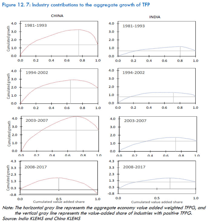 First, neither in India nor in China, the TFP growth has been even in any of the three time periods under consideration. Growth has been uneven in all the periods, although the degree of inequality differs over the periods. While some sectors enjoyed productivity growth, often above their proportional role in the economy, others had a disproportionately large productivity drop. For instance, in the 1980-1993 period, positive contributions from industry TFP growth to aggregate TFP growth added up to 3.3 percentage points in China. In India, they added up to 1.2 percentage points. These positive industries constituted 3/4th of the aggregate GDP in China and 77 per cent in India. Although the proportion of output produced with improving productivity and efficiency was comparable in the two economies, the rate of productivity improvement was far higher in China, by a margin of 2 per cent. The remaining industries that had negative TFPG stripped off 1.8 percentage points from China's aggregate TFPG and 0.55 points from that of India, thus dragging down aggregate TFPG in both countries, respectively, to 1.4 per cent in China and 0.6 per cent in India. In the 1990s, China's positive productivity sectors shrank to 65 per cent of the GDP, and also their TFP summed to a smaller value of 2.9 per cent, 0.3 points lesser than the previous period. India, on the other hand, increased its positive TFPG marginally to 1.3 per cent. However, that was confined to industries that produce less than half the output (see the second panel from the top of Figure 11.7). In other words, while industries that constitute 65 per cent of GDP in China had registered positive productivity growth, only those sectors that constitute 48 per cent of the aggregate economy could do so in India in the 1990s. Indeed, India had a much larger share of industrial production that came less efficiently, with negative TFPG. During 2002-2007, Both countries improved the share of positive TFP industry output to 71 per cent, with an impressive increase in their TFP contribution to 4.3 percentage points in China and a moderate improvement to 1.7 percentage points in India. The drop in aggregate TFPG due to the negative productivity industries was also high in China, by nearly 1.7 percentage points compared to half a percentage point decline in India. Overall, TFPG in China settled at 2.6 per cent, more than double the overall TFPG in India. In the post-crisis period, the output share of industries with positive TFP growth fell in both countries but more intensely in China. While more than half of China's production suffered from a negative TFPG, industries that produce 67 per cent of output in India had positive TFP growth. Moreover, the overall TFP contribution of the positive TFPG industries fell rapidly in China to a mere 1.8 per cent from 4.3 per cent in the previous period. In contrast, India maintained a 1.7 per cent positive TFP contribution. Not only that the negative sectors' share was high in China, but the magnitude of TFPG decline was also much rapid in those industries, thus leading to a much steeper fall in the aggregate TFPG to just above half a per cent. In contrast, with a lesser magnitude of TFP decline in industries that contributed 1/3rd of the output, India managed to avoid a rapid fall in aggregate TFP and thus could sustain a TFP growth of 1 per cent. Thus, despite having a high TFPG in industries with positive TFPG compared to India, the erosion in TFP in other sectors caused China's overall TFP loss in the post-crisis period. | Industries in China and India do not follow a uniform yeast pattern of productivity growth, but rather a mushroom-type pattern—while some industries grow beyond their relative importance in the economy, others underperform | We learn from these charts that industries both in China and India do not follow a uniform yeast pattern of productivity growth. Both countries had an uneven industry pattern of aggregate TFP growth. In other words, they follow a mushroom-type pattern—while some industries grow beyond their relative importance in the economy, others underperform compared to their relative size. In general, the output share of industries that register positive TFPG is higher in China than in India. With higher industry TFP growth and a larger size of the positive TFP sectors, China maintained its productivity edge over India in the 1980s, 1990s, and the pre-crisis years of the 2000s. However, India's TFP growth pattern changed since 2008, when it overtook China, despite many of its industries continuing to perform poorly. The recent magnitude of decline in more than half of Chinese industries has made China's aggregate TFP performance poorer than India's. 12.4.4 Capital deepening and labour productivity growth – a comparative perspective Earlier in this chapter, we discussed the predominant role of capital deepening, or the amount of capital (machines, buildings, computers, etc.) workers work with, in driving the labour productivity growth in India and China and in driving the difference between the two economies. Although capital deepening is an important driver of labour productivity, just investing more in capital may not deliver higher productivity. The productivity effect of capital deepening would rely on the marginal productivity of capital or the elasticity of capital with respect to output. Using the labour productivity version of the standard Cobb-Douglas production function, we compare the productivity impact of capital deepening in India with that of China in Table 11.4. The table provides the results of a panel regression with the log of the labour productivity indices as the dependent variable and the log of capital per worker indices and log of labour quality indices as independent variables, i.e.:  Capital per worker (k) is estimated using the estimated aggregate capital services growth rates and employment growth rate in each industry, and therefore, we use an index version of all variables in the regression. LQ is the index of labour quality. Note that since both capital per worker and labour productivity are indexed to the base year, the estimated constant (γ) in equation (3), that is usually the average log level of TFP in Cobb Douglas estimates, and is hard to interpret. Therefore, we do not attach much significance to the estimated constant in Table 12.4. Our interest is to see whether the capital deepening has a differing impact on labour productivity in the two economies. Note that this regression does not account for any control variables, and therefore, should be considered as indicative results only. The regression is estimated using panel data for the aggregate economy—i.e., across 27 sectors in India and 37 sectors in China, over the period 1980-2017—and separately for manufacturing and market services sectors. We provide both the random effects and fixed effects results in the table. The Hausmann statistics fail to reject the null hypothesis that a random effect model is appropriate in the case of all the three sectors in India. For China, however, a fixed-effect model is preferred for the aggregate economy and manufacturing sector, whereas a random effects model is not rejected for the market services sector. Therefore, our discussions will be based on the random effects model results for all sectors in India and the market services sector in China. The fixed-effects model will be used for the aggregate economy and manufacturing sector in China. However, in general, the magnitude of the difference between the two models, both within the individual economies and the comparative picture of the two economies is quite negligible. | Our discussions are based on the random effects model results for all sectors in India and the market services sector in China. The fixed-effects model is used for the aggregate economy and manufacturing sector in China |
| Table 12.4: Regression estimates- Dependent variable: log of labour productivity (indexed to the base year) | | | Fixed Effects | Random effects | | All sectors | Manufacturing | Market services | All sectors | Manufacturing | Market services | | India | | Capital per worker | 0.379*** | 0.413*** | 0.248*** | 0.374*** | 0.405*** | 0.258*** | | | (15.94) | (12.31) | (8.10) | (16.00) | (12.30) | (8.60) | | Labour quality | 2.291*** | 1.859*** | 5.299*** | 2.315*** | 1.913*** | 5.214*** | | | (13.55) | (7.90) | (19.67) | (13.90) | (8.28) | (19.66) | | Constant | -7.715*** | -5.912*** | -21.01*** | -7.806*** | -6.124*** | -20.66*** | | | (-11.05) | (-6.11) | (-18.32) | (-11.28) | (-6.40) | (-18.25) | | Nr. of observation | 874 | 494 | 228 | 874 | 494 | 228 | | R-square | | | | | | | | Within | 0.744 | 0.718 | 0.897 | 0.744 | 0.718 | 0.897 | | Between | 0.282 | 0.214 | 0.246 | 0.283 | 0.220 | 0.268 | | Overall | 0.558 | 0.512 | 0.834 | 0.559 | 0.515 | 0.836 | | China | | Capital per worker | 0.821*** | 0.985*** | 0.429*** | 0.815*** | 0.977*** | 0.424*** | | | (39.53) | (38.92) | (11.72) | (39.22) | (38.26) | (11.67) | | Labour quality | 1.078*** | 1.532*** | 2.038*** | 1.093*** | 1.562*** | 2.061*** | | | (7.12) | (6.01) | (12.15) | (7.20) | (6.07) | (12.34) | | Constant | -3.978*** | -6.890*** | -6.190*** | -4.017*** | -6.987*** | -6.269*** | | | (-6.15) | (-6.24) | (-8.72) | (-5.96) | (-6.11) | (-8.53) | | Nr. of observation | 1254 | 722 | 266 | 1254 | 722 | 266 | | R-square | | | | | | | | Within | 0.716 | 0.811 | 0.708 | 0.716 | 0.811 | 0.708 | | Between | 0.004 | 0.051 | 0.272 | 0.004 | 0.051 | 0.277 | | Overall | 0.192 | 0.163 | 0.548 | 0.192 | 0.163 | 0.551 | Note: *** significance at 1%; ** significance at 5%; and * significance at 10%.
Source: India KLEMS and China KLEMS | We see that the estimated coefficient of capital deepening is higher in China, in general (Table 12.4). One per cent higher capital per worker leads to about 0.38 per cent labour productivity in India and 0.82 per cent in China. In other words, the elasticity of capital in China is far higher than in India. It may also be noted that the estimated elasticity is higher than the actual share of capital income in value added in China and lower in India—for the 1980-2017 period, it averaged at about 52 per cent in both economies. A few important insights from the table are first, the relative impact of capital deepening on labour productivity in China is much higher in manufacturing than in market services. Second, the difference between the productivity impact of capital deepening in manufacturing and market services is relatively low in India compared with China. The impact in the manufacturing sector is higher by 0.15 points in India, whereas it is higher by 0.6 points in China compared to the market services sector. Third, the productivity impact of labour quality is much higher in both countries in market services than in manufacturing, which is likely due to the presence of more skill-intensive jobs in this sector. Fourth, in both sectors, India has a better labour quality coefficient, and the gap between the two economies is much larger in market services. Overall, we see a clear pattern. The Chinese economy, especially its manufacturing sector, seems to have seen much success in creating productivity by investing in physical capital compared with India. In other words, the marginal productivity of capital has been higher in Chinese manufacturing. The same was the case with market services, and thereby the overall market economy, although the difference between India and China in the market services sector was less intense than in the manufacturing sector. In contrast, upskilling its workers has a larger productivity impact in India, primarily in its market services, compared to China. The capital-driven growth in China's manufacturing and skill-driven growth in India's market services is clearly seen in terms of the marginal productivity effects of these inputs in the two economies. 12.5 Conclusion Economic growth in India and China has been widely discussed in recent literature, as these giant economies have been the major driving force of global growth. The two economies share the experience of a shift from a socialist past to a market economy, which happened around the early 1990s. However, their growth journeys have been quite different. While China's growth was largely driven by the manufacturing sector, India relied substantially on its services sector. This chapter compares the proximate sources of economic growth in the two countries, i.e., the role of capital accumulation and total factor productivity in driving labour productivity, using a comparable methodology and detailed industry-level data. We cover the period of 1980-2017, divided into three sub-periods 1980-92, 1993-2002, 2003-17, broadly consistent with major policy changes in the two economies. The last period, 2003-07, has been further sub-divided into pre-crisis and post-crisis, with 2007 as the cut-off year. We observe several important trends. Although labour productivity in India and China is still far below the global frontiers, both these countries have substantially improved their relative productivity performance during their post-market reform period. Regardless, they still have a long road to go, as their productivity levels are still the lowest compared to other emerging market peers. China's labour productivity has grown much faster than India over the last 40 years, widening the gap between the two countries. A massive tide in its non-service economy has driven China's faster labour productivity growth compared to India, where the service economy has done relatively better. China performed relatively better in all the nine industry groups considered in the chapter, except the financial and business services sectors in the 1994-2002 period and non-market services through the entire 1981-2017 period. The difference was immense during the 1994-2002 period in most industry groups. China's dominance in the industrial sector is also visible in its TFP performance. China did better in the aggregate economy, agriculture, and industry, whereas its performance in the service sector was much worse than in India. | While the output share of industries with productivity increase is high in China for the entire period, that dominance was eroded substantially since the global financial crisis. The scale of decline in TFPG for over half of China’s industries made its aggregate performance poorer than India's since 2008. | Our analysis of the industry pattern of aggregate TFPG in China and India further reveals that both experienced an uneven pattern of aggregate TFP growth with TFPG in some industries growing beyond their relative importance in the economy and others underperforming. Although in general, the output share of industries with productivity expansion has been high in China throughout the entire period, that dominance has eroded substantially since the global financial crisis. The magnitude of decline in more than half of Chinese industries' TFPG has made China's aggregate TFP performance poorer than India's since 2008. Finally, our analysis of the productivity effect of investment in physical capital suggests that the Chinese manufacturing sector was significantly more successful in increasing productivity by investing in physical capital than its Indian counterpart. The marginal productivity of capital has evidently been higher in Chinese manufacturing. As well-established in the literature, India's growth and productivity have been driven by the services sector, and our results indicate that more than capital deepening, it was the skill intensity of workers that appears to have had a higher marginal impact on labour productivity in its market services sector. Clearly, upskilling its workers had a larger productivity impact in India, primarily in its market services, compared to China. The capital-driven nature of growth in China's manufacturing and skill-driven growth in India's market services is visible in terms of the marginal productivity effects of these inputs in the two economies. Our findings reinforce the observation of a recent study by Ghose (2019) that the divergence in the pace and pattern of growth between India and China since the 1980s is an outcome of China's rapid progress in investing in physical and human capital. While China was already prepared for take-off by the 1970s, India's lack of focus on primary education curtailed its progress. Ghose (2019) also argues that a well-defined sector-oriented growth strategy in China was largely helpful in achieving higher growth in agriculture and manufacturing. The analysis conducted in this chapter is the most comprehensive comparison of India and China in terms of productivity growth, including the post-global financial crisis period. However, considering other recent studies that compared India and China using the KLEMS data (e.g., Wu et al., 2017) and separately analysed these countries (Erumban and Das, Wu 2020), the productivity estimates in this study need further methodological improvement. This is because the current study uses a value-added function, which disregards the role of intermediate inputs in deciding the growth rate of industry-level total factor productivity. This has also forced us to use industry value-added shares while aggregating productivity growth across sectors to industry groups, broad sectors, and aggregate economy, compared to a more accurate Domar weight. Subsequent analysis should consider comparing productivity growth between the two economies using a gross output function at the industry level and examine the trend in productivity in the most recent period in context of previous findings in Wu et al. (2017). | Our productivity estimates need further methodological improvement because the current study uses a value-added function, which disregards the role of intermediate inputs in deciding the growth rate of industry-level total factor productivity. | Annexure 12A: India KLEMS and China KLEMS, Concordance | Table 12A.1: Industries in India KLEMS and China KLEMS and their concordance with industry groupings | | China CIP/KLEMS | India KLEMS | Industry groupings | Broad sectors | | 1. Agriculture, Forestry, Animal Husbandry & Fishery | 1. Agriculture, Hunting, Forestry & Fishing | 1. Agriculture | 1. Agriculture | 2. Coal mining
3. Oil & gas extraction
4. Metal mining
5. Non-metallic minerals mining | 2. Mining & Quarrying | 2. Other goods production | 2. Industry | 6. Food & kindred products
7. Tobacco products | 3. Food Products, Beverages & Tobacco | 3. Consumer & intermediate goods manufacturing | 8. Textile mill products
9. Apparel & other textile products
10. Leather & leather products | 4. Textiles, Textile Products, Leather & Footwear | | 11. Saw mill products, furniture, fixtures | 5. Wood & Products of wood | | 12. Paper products, printing & publishing | 6. Pulp, Paper, Paper products, Printing & Publishing | | 13. Petroleum & coal products | 7. Coke, Refined Petroleum Products & Nuclear fuel | | 14. Chemicals & allied products | 8. Chemicals & Chemical Products | | 15. Rubber & plastics products | 9. Rubber & Plastic Products | | 16. Stone, clay, & glass products | 10. Other Non-Metallic Mineral Products | 17. Primary & fabricated metal industries
18. Metal products (excl. rolling products) | 11. Basic Metals & Fabricated Metal Products | | 19. Industrial machinery & equipment | 12. Machinery, nec. | 4. Investment goods manufacturing | 20. Electric equipment
21. Electronic & telecomminucation equipment
22. Instruments & office equipment | 13. Electrical & Optical Equipment | | 23. Motor vehicles & other transportation equipment | 14. Transport Equipment | | 24. Miscellaneous manufacturing industries | 15. Manufacturing, nec; recycling | 3. Consumer & intermediate goods manufacturing | | 25. Power, steam, gas & tap water supply | 16. Electricity, Gas & Water Supply | 2. Other goods production | | 26. Construction | 17. Construction | | 27. Wholesale & Retail Trades | 18. Trade | 5. Trade and distribution | 3. Services | | 28. Hotels & Restaurants | 19. Hotels & Restaurants | 8. Other market services | | 29. Transport & Storage | 20. Transport & Storage | 5. Trade and distribution | | 30. Post & Telecommunications | 21. Post & Telecommunication | 8. Other market services | | 31. Financial Intermediation | 22. Financial Services | 6. Finance services | | 33. Leasing, Technical, Science & Business Services | 23. Business Service | 7. Business Services | | 34. Public Administration & Defense | 24. Public Administration & Defense; Compulsory Social Security | 9. Non-market services | | 35. Education | 25. Education | | 36. Health & Social Security | 26. Health & Social Work | 32. Real Estate Activities
37. Other Services | 27. Other services | | Total Economy | Total Economy | Total Economy | Total Economy | Chapter 13: Summary and Conclusion 13.1 The context This chapter seeks to summarise the report’s main findings and their implications as well as to suggest directions for the India KLEMS database and associated research in the future. The main purpose of the report was to analyse the growth and productivity of the Indian economy with the help of the KLEMS database. It has considered several dimensions of India’s growth and productivity since 1980s and how these evolved over the period 1980-2017. The phases that marked this period are (i) the partial and major reforms of the 1980s and 1990s, (ii) high growth episodes of the 2000s and (iii) the global slowdown post 2008. The report’s core chapters provide a comprehensive analysis of the trends in primary inputs – labour and capital – and intermediate inputs, along with analysis of economic growth and productivity in India over the last three decades that enables an evaluation of the sources of growth of the Indian economy and related dimensions since the 1980s. The main methodology used is the growth accounting approach that allows the decomposition of output growth into growth of inputs and productivity growth. By doing so, we trace the sources of growth in output to increased investment in capital goods, increased use of labour, increased use of intermediate inputs or increases in efficiency with which inputs are combined to outputs. The analysis was undertaken at a detailed level of industry disaggregation (two-digit industries or thereabout) using the India KLEMS database that provided internationally comparable and harmonised statistics on inputs, outputs and productivity for 27 sub-industries. The emphasis on the disaggregated approach adopted here allows a detailed understanding of the dynamics at the industry level, which is not possible with the aggregate economy level approach. The novelty of our approach lies in the assessment of contributions of industries to aggregate growth based on an in-depth analysis of data for 27 industries comprising the Indian economy. This chapter has seven sections that provide summaries of major findings of all chapters, organized by the main themes addressed. The main findings pertain to our examination of input versus efficiency considerations in the economy’s growth. Second, both labour and total factor productivity of the aggregate economy and the industry origins of the overall growth and productivity performances have been studied. Third, both manufacturing and services have been examined in detail with a focus on growth and productivity. In addition, various aspects of the formal-informal divide were examined for manufacturing industries and of factor intensities in various manufacturing and non-manufacturing industries. The issue of services-led growth was examined for market and non-market service categories and their contribution to the service economy as well as the aggregate economy. The report ends with a discussion comparing growth and productivity of India and China. | The novelty of our approach lies in the assessment of contributions of industries to aggregate growth based on an in-depth analysis of data for 27 industries comprising the Indian economy. | 13.2 Outputs and Inputs Following the discussion on the construction of the India KLEMS database in Chapter 2, the three subsequent chapters analysed trends in output (value added and gross output) and inputs (primary and intermediate inputs). These analyses were carried out at the levels of the aggregate economy and the broad sectors, and for 27 industries comprising the economy. 13.2.1 Output, value added and intermediate inputs On the output side, real value added of the aggregate Indian economy, according to our measurement, grew at the rate of 6 per cent per annum during the period of study, 1981 to 2017, and the growth rate improved over the sub periods until the financial crisis beginning 2007-08. The value-added growth for the aggregate economy was between 5 to 6 per cent in the period 1981 to 2002, which improved to 7.7 per cent during 2003-07 (as observed in several previous studies on India’s economic growth) and then declined to 6.4 per cent for the sub-period 2008-17. | Our analysis reveals that the effect of the financial crisis on value added was much more prominent at the disaggregated industry level. As many as 19 out of 27 industries experienced a decline in growth rate after the financial crisis of 2007-08. | The growth rate of output varied across industries ranging from 1.16 per cent in wood & wood products to 12.4 per cent in business services. In terms of broad sectors, services sector grew at a faster annual rate (7.3 per cent) than others, while agriculture grew at a much slower annual rate (3.1 per cent). Within the services sector, market services such as business services, post & telecommunication, and financial services registered faster growth than non-market services including health & social work, education, and public administration. In the case of manufacturing, electrical & optical equipment, rubber & plastic products, coke & petroleum products and transport equipment observed a higher growth rate than other industries. Our analysis reveals that the effect of the financial crisis on value added was much more prominent at the disaggregated industry level. As many as 19 out of 27 industries experienced a decline in growth rate after the financial crisis of 2007-08. Moving on to intermediate inputs, we find that their contribution to growth in gross output is high—with the contribution of material inputs to output growth higher than that of other factors of production. It is as high as 40-50 per cent in the manufacturing sector, while the contribution of service inputs to growth in gross output lies between 10 to 20 per cent. Evidently, material input has been the dominant source of output growth for most industries. Therefore, intermediate inputs play a crucial role in explaining economic growth at the industry level. 13.2.2 Labour input and labour income share The structure of employment saw a significant change in the Indian economy between 1980 and 2017. The share of agriculture reduced in total employment from 70 to 42 per cent and the share of the services sector doubled from 17 to 34 per cent, leaving the share of manufacturing stagnant around 11 per cent. The average annual growth in employment in India during the period of 1981-2017 was 1.3 per cent. The sub periods spanning the 1990s and major part of the 2000s saw a similar low growth rate of around 1.3 per cent per annum, in contrast with the relatively higher 2.1 per cent growth rate in the 1980s. The period 2008-17 saw almost no growth in employment. The workforce participation rate (WFPR) in India declined from 38.6 per cent in 2011-12 to 34.7 per cent in 2017-18, which is consistent with the observation of almost no employment growth during 2008-17; rather a fall is found. The decline was evident for both rural and urban sectors. The WFPR has remained consistently low for the female workforce. | The workforce participation rate (WFPR) in India declined from 38.6 per cent in 2011-12 to 34.7 per cent in 2017-18, which is consistent with the observation of almost no employment growth during 2008-17 | The labour income share in India had declined from 1980 to 2008, similar to the experience of many other countries. Nevertheless, it showed a tendency to increase between 2008 and 2017, mainly due to the faster growth in real wages as compared with labour productivity growth. The change in the aggregate economy level labour income share seems to be mainly a within-industry effect than a structural change effect. The average growth in the labour quality index, a measure of change in skill composition of workers during the period 1981-2017 has been 1.2 per cent per annum. Further, we observe a rise in the share of high skilled labour193 (with education above secondary schools) from a mere 2.4 per cent to almost 13 per cent and a simultaneous decrease in the proportion of employed persons with level of education with below primary level from 70 per cent to 32 per cent. Although manufacturing has not been the major contributor to employment growth, the average annual growth in employment in the manufacturing sector was above average at 1.6 per cent, compared with 1.3 per cent for the total economy during 1981-2017. However, the average growth in labour quality index in manufacturing was close (1.2 per cent) to that for the total economy (1.1 per cent) during 1981-2017. The highest growth in employment in this period was observed for the following industries: business services, construction, electrical and optical equipment, financial services, and machinery, n.e.c. The laggards in this regard were agriculture, public administration and defence, wood & products of wood, textiles etc., and mining & quarrying. Industries which showed the highest growth in labour quality index were chemicals and chemical products, mining & quarrying, machinery, n.e.c., and transport equipment. Industries with the slowest growth in labour quality were wood & wood products, agriculture, business services, construction and financial services. It is evident from the employment conditions that India needs to focus on both the demand and the supply side of employment. On the demand side, the industries with relatively high employment-generating capacity need to be encouraged, along with development of relevant skills and promotion of suitable techniques of production. On the supply side, policymaking has to support greater participation of women in the workforce in order to increase the supply of labour and encourage upskilling of the population. A striking feature of employment trends in India in the recent period is a decline between 2011 and 2017, in aggregate employment and in employment in agriculture and manufacturing. Since the growth rate of real GVA of manufacturing was fairly high at about 7.2 per cent per annum during this period, a decline in employment in manufacturing appears puzzling. It should be pointed out here that there are issues regarding the comparability of various employment surveys, particularly while combining the EUS (Employment Unemployment Survey) and PLFS (Periodic Labour Force Survey), as was done in this analysis. This may also have implications for the recent fall in employment growth observed between 2011 and 2017 in the data. However, our econometric analysis provides some credibility to our stand that it is appropriate to combine EUS with PLFS for construction of labour input series for the recent period, as the model estimates predict a fall in employment during this period in agriculture, industry (excluding construction), and the aggregate economy, which is in line with the actual fall indicated by EUS and PLFS. | Since the growth rate of real GVA of manufacturing was fairly high at about 7.2 per cent per annum during 2011-17, a decline in employment in manufacturing during the same period appears puzzling. | The recent trends in employment statistics in India indicate a relatively high unemployment rate, especially among the youth, in the last year of our analysis. The youth in rural areas belonging to relatively poorer households are now less inclined and less under compulsion to join labour force than was the situation in the beginning of the 2010s. They would rather stay unemployed than take up a low-paying, low-quality job. Moreover, we also observe a fall in employment trends in the manufacturing sector, indicating the sector's failure in absorbing workers moving out of agriculture. 13.2.3 Capital input 13.2.3 Capital input The chapter on capital input (Chapter 5) discussed the trends in investment/GDP ratio, real investment, capital stock, and capital service growth rates in the 27 KLEMS industries during the period of study. A unique feature of the analysis in this chapter, when compared with several previous studies on productivity (see Ahluwalia, 1991; Balakrishnan and Pushpangadan, 1994; Goldar, 2004, among others), is the use of capital services, which takes the heterogeneity of capital assets into account. We distinguish three types of assets, a slow depreciating asset of construction (or buildings) and fast depreciating assets of machinery and transport equipment. The chapter observes an improving aggregate investment growth over the three sub-periods—1981 to 1993, 1994 to 2002, and 2003 to 2017. The fastest investment growth was observed in the 2000s, a period when the Indian economy was growing rapidly. Two broad sectors—construction and market services—were the main drivers of the high investment growth in the 2000s, although all other broad sectors of the economy, including manufacturing, also grew rapidly during this period. Considering the pace of investment growth across the three asset types, it was observed that the rapid increase in equipment investment facilitated the faster growth in total investment in the 2000s. The growth of equipment investment accelerated across the board, although there were substantial differences across sectors in terms of levels and growth rates. For instance, non-market services and agriculture sectors, despite seeing a consistent increase in the equipment share, maintained a relatively low presence of equipment capital compared with manufacturing, construction, and market services. Regardless, the chapter observed an increasing role of equipment capital in the economy, which helped improve capital composition effects. Capital composition effects are the impact of investment moving towards higher productivity assets, on production, and such impact is generally observed to be positive.194 | The fastest investment growth was observed in the 2000s, a period when the Indian economy was growing rapidly, —construction and market services—were the main drivers. A rapid increase in equipment investment facilitated this rapid growth in total investment. | 13.3 Labour Productivity and Total Factor Productivity Chapters 6 and 7 extensively analyse both—labour productivity and total factor productivity for the entire economy, broad sectors as well as disaggregated 27 industries for the period 1980-2017 and the sub periods. The study comes up with several important findings: (i) The growth of labour productivity varies across industries. Chemical and chemical products grew the fastest with an annual growth rate of more than 6 per cent, followed by other non-metallic mineral products; public administration; post & telecommunication; and textile & leather products. At the other end were construction; wood and wood products; machinery, n.e.c..; other services; transport & storage; and pulp, paper, etc. which recorded very low (less than 3 per cent) growth in labour productivity. The change in labour productivity growth rate between the periods of 1994 to 2007 and 2008 to 2017 also varied considerably. (ii) The analysis also reveals that labour productivity growth was faster in high capital-intensive industries and in ICT-producing and ICT-using industries compared with non-ICT industries. (iii) The analysis of drivers of growth in labour productivity indicates that capital deepening is a significant contributor to the observed labour productivity growth, leaving the contribution of growth in labour composition as well as of TFP growth relatively small. | Industry decomposition of labour productivity growth shows that aggregate productivity growth was explained majorly by within-industry productivity growth, and between-effect or structural change remained relatively a small contributor | Industry decomposition of labour productivity growth shows that aggregate productivity growth was explained majorly by within-industry productivity growth, and between-effect or structural change remained relatively a small contributor. The static reallocation effect which indicates the movement of workers to sectors with relatively better levels of productivity has been positive and is 25 per cent of the aggregate productivity growth in the period 1981-2017, suggesting a positive structural change effect. The dynamic effect which indicates the movement of workers to sectors with relatively faster productivity growth has been mostly negligible suggesting that employment has hardly been generated in sectors which were witnessing faster productivity growth. The analysis also makes it very clear that the major contribution to the aggregate productivity growth has come from the service sector in all the sub-periods, especially immediately after the reform process had begun in India in 1990’s, and in 2008-17. A cross-country comparison, however, reveals that despite achieving one of the highest annual growth rates in labour productivity at an average of 5 per cent during 1981-2017, the level of labour productivity in India is still very low compared with other selected countries. On comparing with China, it was found that while India and China had almost the same level of labour productivity in 1980, the level in India had become three-fourths of that in China by 2018. The analysis of industry-level output growth rates for 1981-2017 reveals that the output growth rates for the 27 India KLEMS industries follow a normal distribution, with a majority of the industries recording an annual output growth rate closer to the all-industry mean of 7.39 per cent.195 Among the few industries that saw output growth rates higher than the all-industry mean, business services saw the relatively highest annual growth of 12.4 per cent. Decomposition of industry-level output growth for 1981-2017 reveals that intermediate inputs were by far the largest contributors with an industry mean of 4.16 ppts. Within intermediate inputs, much of the contribution was driven by material (M) input, especially for the industries belonging to the manufacturing sector. The contribution from services input was substantial for agriculture & allied, utilities and six industries belonging to the services sector, indicating the importance of intermediate transactions in these sectors. Capital input was the second most important contributor, especially for services such as trade, business services and financial services, indicating the important role of investment in physical assets in these industries. | Contributions from TFP growth were negligible for output growth in the majority of the industries. Input accumulation drove output growth rates in the Indian economy during the 1981-2017 period, rather than improvements in efficiency. | The labour input contribution to output growth was very minor with an industry average of 0.78 per cent per annum. The quality components of the primary inputs i.e., the contribution from capital and labour quality were marginal for the overall period. However, labour quality was the dominant source of labour input contribution for four industries—public administration, wood & wood products, mining & quarrying, and agriculture & allied, mostly due to the little to no employment growth in these industries in comparison with favourable labour quality growth rates, for the overall period. Finally, we find that TFP contribution to output growth (or simply gross output based TFP growth rates) also follow a normal distribution with most of the growth rates near the industry average of 0.47 per cent per annum.196 The contributions from TFP growth were negligible for the majority of the industries. Overall, for the 1981-2017 period, we observe that input accumulation drove output growth rates in the Indian economy rather than improvements in efficiency. We observe that the largest contributors to aggregate value-added growth for the overall period include agriculture & allied industries and services—trade, other services, business services and financial services. While the contribution from the agriculture & allied sector was largely due to its high value-added share in aggregate value-added (25 per cent), the contributions from the above-mentioned services industries reflected their strong value-added shares and high value-added growth. Strikingly, manufacturing industries performed poorly in terms of their contributions—raising questions about the success of various economic policies initiated to expand the manufacturing sector. The method of Direct Aggregation across Industries (DAI) allowed the incorporation of the ingenious method of Domar aggregation. From this exercise, we find that the agriculture & allied and public administration industries made the largest contributions to aggregate TFP growth for the overall period of 1981-2017. As discussed in the chapter dealing with productivity growth, the TFP growth in public administration should be treated with caution. The DAI approach also allowed us to analyse industry contributions to the growth of aggregate primary inputs. For the overall period, this exercise revealed that services were large contributors to aggregate growth of both capital and labour input. The relatively lower contribution from the manufacturing industries towards aggregate labour input growth is again a matter of concern and reflects the poor employment growth in this sector. | For the overall period, services were large contributors to aggregate growth of both capital and labour input. The relatively lower contribution from manufacturing towards aggregate labour input growth is a matter of concern and reflects the poor employment growth in this sector. | Looking at the pre and post Global Financial Crisis (GFC) growth and productivity dynamics, we find a revival of TFP growth for 12 industries, mainly those belonging to capital-intensive manufacturing and non-market services. This could be a possible reflection of poor global integration of these industries, which insulated them from the volatility of the GFC. Importantly, although the spread in the changes of labour input contributions were small in absolute magnitude, 23 out of the 27 India KLEMS industries saw a deceleration in labour input contribution over the two sub-periods. A post-2007 acceleration in contributions to aggregate value-added growth was observed for five service sector industries. Further, while the contribution to aggregate TFP growth from market services declined post 2007, the corresponding contribution from capital-intensive manufacturing industries accelerated. The large post-2007 increase in capital input growth in the trade industry caused a substantial increase in its contribution to aggregate capital input growth in the second sub-period. Finally, it is found that 19 out of the 27 India KLEMS industries saw a decline in their contribution to aggregate labour input growth in the second sub-period, with the largest decline seen in contributions from the agriculture & allied sector and trade industry. In order to provide an overview of the disaggregated analysis for expositional clarity, the chapter on productivity growth also undertook a sectoral analysis of growth and productivity. For the overall period of 1981-2017, it is observed that although the manufacturing sector saw higher value-added growth than services, the relatively higher value-added share of the latter led to a relatively larger contribution to aggregate value-added growth (as judged from the analysis based on the PPF {production possibility frontier} approach). Notably, the service sector contribution to aggregate value-added growth was driven mostly by contributions from the market services sub-sector. However, market services saw the largest decline in contributions to aggregate value-added growth over the two sub-periods of 1993-07 and 2008-17. On the other hand, non-market services saw a corresponding increase in contribution. The manufacturing sector saw a substantial increase in its contribution, primarily driven by the large increase in contribution from the manufacturing of intermediate goods. Finally, we find that aggregate TFP growth for the overall period primarily reflects intra-industry TFP growth from the component industries within the aggregated sectors. However, positive reallocation effects from labour and capital were also observed at 0.59 and 0.54 per cent, respectively (to be contrasted with the within-industry effect of 0.96 per cent, together comprising the 2.09 per cent growth rate in TFP). As in the case of sectoral contributions to aggregate value-added growth, over the two sub-periods, the contribution of non-market services to aggregate TFP growth increased, while there was a decline in the corresponding contribution from market services. Interestingly, the manufacturing sector as a whole saw the largest increase in contribution to aggregate TFP growth—possibly implying that this sector was somehow insulated from the volatility of the post-GFC period. 13.4 The Performance of Manufacturing – formal-informal divide and energy use Manufacturing has always been remained important for India’s growth aspiration and this is reflected via policies that have been put in place since the 1950s. Chapter 8 and the first half of Chapter 9 deal with an examination of manufacturing performance especially issues such as the formal-informal divide and energy intensity. Although India’s manufacturing sector played an important role by contributing 18 per cent to value added and 11.5 per cent to employment in 2017-18, these shares were virtually stagnant, especially for employment. Because of the stagnation in its relative share in the Indian economy, the growth of manufacturing has been the focus of the policy makers and both, the manufacturing policy of 2011 and the ‘Make in India’ programme in 2014 were designed to promote faster growth of this sector. | Although India’s manufacturing sector played an important role by contributing 18 per cent to value added and 11.5 per cent to employment in 2017-18, these shares were virtually stagnant, especially for employment | 13.4.1 Formal-Informal Divide Manufacturing in India has a dualistic structure with the organised and unorganised segments, which could be called formal and informal sectors within manufacturing. The unorganised sector has played an important role and has one-third share in GVA but two-third share in employment in 2017-18. These shares persisted between the period of 1999 and 2017, with growth in real GVA of 7.17 per cent in the unorganised sector as compared with 7.26 per cent in the organised sector. The growth in unorganised sector real GVA accelerated from 5.6 per cent during 2000-2007 to 8.5 per cent during 2008-17. On the other hand, the growth in employment during 2000-2017 in the unorganised sector has been much lower (0.46 per cent) as compared with the organised sector (2.72 per cent). As a result, the organised sector accounted for 7 million of total employment addition of 10 million in manufacturing during the period. It is observed that both the organised and the unorganised segments of the 13 manufacturing industries have disparateness in the growth of GVA and employment. Because of such differences in the 13 manufacturing industries, we also observe significant variation in the level and growth in labour productivity across industries and over time. Labour productivity in the unorganised manufacturing segment has always been lower than that of the organised segment, though the relative difference has narrowed down over time. Thus, the unorganised segment has always exerted downward pressure—a drag—on labour productivity of the manufacturing sector as well as its constituent 13 industries. The drag is more than 25 per cent of the aggregate labour productivity growth without informality, and it is slightly higher in the second sub-period of 2008-17. The decomposition of the labour productivity growth shows positive structural (or between-industry) change and positive within-industry change, thus pointing to the phenomenon of movement of workers from less productive to more productive industries as well as from less productive segment to more productive segment within an industry. This phenomenon along with an increase in employment in the organised sector augers well for the Indian economy in its quest for ‘formalisation’. | Decomposition of labour productivity growth shows positive values for structural and within-industry change, pointing to the movement of workers from less productive to more productive industries as well as from less productive segment to more productive segment within an industry | A close analysis of the 13 industries may identify more policy options whereby focus could be laid more on industries that could aid in accelerating the process of formalisation of Indian manufacturing from both capital and labour points of view. It is important that impediments to the growth of the organised manufacturing sector be removed by taking appropriate policy initiatives to accelerate its growth. The enterprises in the unorganised sector must also be incentivised to grow and compete by removing obstacles through the provisioning of cheap finance, regular supply of electricity and other necessary inputs, access to new appropriate technology and markets. It needs to be reiterated that while organised manufacturing achieved modest growth in employment during 2008-17, there was a fall in employment in unorganised manufacturing. Within the unorganised manufacturing sector, it is the ‘establishments’ where employment declined between 2010 and 2015, while employment in own account enterprises (which do not have any hired workers and are relatively smaller in size than establishments) did not fall (Dandapat, et al. 2021). We have not investigated the reasons for the fall in employment in informal manufacturing, particularly among ‘establishments’ in the period 2008-17. However, evidently, it would not be wrong to say that a tendency towards growing formalisation of industrial enterprises in India may have had an adverse effect on the growth of employment in India’s unorganised manufacturing segment. Another possibility is that with improving living standards, Indian consumers are increasingly demanding better product quality and turning more brand conscious. This might have eroded—to some extent—the competitiveness of informal manufacturing enterprises since their competitive advantage primarily lies in terms of pricing, rather than product quality. 13.4.2 Energy intensity of manufacturing The analysis of trends in energy intensity in manufacturing revealed a downward trend in the period from the 1980s till the end of the 2000s, and a trend reversal or a slowing of the prevailing downward trend since 2011. Econometric analysis of determinants of energy use and energy intensity presented in Chapter 10 revealed a significant negative relationship between energy price and energy demand in manufacturing. An examination of movements in real price of energy revealed that there was a fall in real price of energy input in manufacturing in the period 2011-17 and this could be one of the important factors that arrested or slowed the prevailing downward trend in energy intensity in manufacturing. Supplementary econometric analysis of energy intensity trends in Indian manufacturing at the aggregate level with the help of time series data revealed that while output had a positive effect on energy consumption, export intensity of Indian manufacturing had a negative effect on energy intensity. This analysis, based on time series data for aggregate manufacturing, also indicated that since 2011 there were probably several factors that tended to push up the energy intensity—with the fall in real price of energy being one of them. | The finding that the earlier downward trend in energy consumption in manufacturing halted during 2011-17 (possibly an indication of the subsequent trend post 2017 and the likely trend in the future) is a matter of concern in view of India’s commitment to cut down its emissions intensity | Manufacturing accounts for a little over half of energy consumption of the Indian economy, and the finding that the prevailing downward trend in energy consumption in manufacturing had halted during 2011-17 (possibly an indication of the subsequent trend post 2017 and the likely trend in the future) is a matter of concern in view of India’s commitment to cut down its emissions intensity—the goal for which has recently been enhanced. Policy action is thus needed to encourage energy conservation in manufacturing. 13.5 Capital intensity: A relook at the trends and underlying factors Chapter 9 discussed trends in capital intensity and suggested a possible impact of factor prices on capital intensity. The chapter observed that the Indian economy is increasingly becoming more capital intensive, substantiating earlier findings in the context of the manufacturing sector increasingly using more capital-intensive technologies compared with other countries such as China (Hasan et al., 2013). Capital intensity has been rising in India as the relative price of capital has been falling relative to workers’ wages, apparently making the substitution of labour by capital more attractive to firms. This observation was reinforced through econometric analysis, establishing a positive relationship between wage/rental ratio and capital per worker ratio in the aggregate economy. Similar observations about the rising wage/rental ratio leading to lower labour intensity in India's manufacturing can be seen in Sen and Das (2015). Many factors, including subsidised technology up-gradation, low custom duties for export-intensive sectors, and rigidities in the labour market, are identified as major factors for capital deepening in the manufacturing sector (Hasan et al., 2013). However, the high capital-output ratio in Indian industries does not appear to be productivity-enhancing, as observed by a recent study by Khanna and Sharma (2021) using the India KLEMS database. While previous studies have considered the efficiency of capital from an aggregate capital stock perspective, it may be worth exploring that relationship further in the context of the rising share of equipment capital in several industries. | The manufacturing sector sees rapid expansion in its capital per worker ratio. Yet, it remains a puzzling case, as the sector’s relative price of labour is one of the lowest when compared with other broad sectors, which is a unique finding in this report. The dynamics in capital intensity and its effect on productivity in industries beyond the manufacturing sector, warrant further research. | Moreover, most previous studies (Khanna and Sharma, 2021 being an exception) that considered the role of capital intensity in India confined their analysis to manufacturing, specifically the organised manufacturing sector. The analysis in Chapter 9 covered all sectors of the economy, and the results indicated that much of the recent expansion in capital services and capital deepening happened in the market services and construction sectors. Also, a simple comparison of capital intensity growth and labour productivity growth between the 1990s and 2000s in Chapter 9 of this report did not indicate a strong positive association between the two. Therefore, the dynamics in capital intensity and its effect on productivity in various industries, going beyond the manufacturing sector, warrant further research in the future. Indeed, as observed by previous studies, the manufacturing sector also sees a rapid expansion in capital per worker ratio. Yet, it remains a puzzling case, as the relative price of labour in this sector is one of the lowest when compared with other broad sectors of the economy, which is a unique finding in this report. This makes the question of jobless growth in India's manufacturing (Bhalotra, 1998; Tejani, 2015; Verma, 2012, among others) an even more intriguing question. A comparison of the rising capital intensity in the construction sector with its substantially weak productivity performance also makes us tentatively conclude that the sector fails to translate its disproportionate use of capital into productivity, which is a subject that needs further scrutiny. Earlier research has shown that the construction boom in the Indian economy accompanies a fall in real wages in the sector as the reallocation of workers (largely unskilled workers) from the primary sector adds little to the sector's productivity (Erumban and Das, 2019). Our analysis revealed that the growth rate in capital intensity 1981-2017 was relatively much higher in the following industries: mining and quarrying; textiles, textile products, leather & footwear; coke, refined petroleum products & nuclear fuel; other non-metallic mineral products; trade; education; and health & social work. However, the growth rate in capital intensity was relatively low (even negative in one case) in the following industries: pulp, paper, paper products, printing & publishing; electrical & optical equipment; transport & storage; financial services; and ‘other services’. Regarding the trends at the aggregate economy level, the annual growth rate in capital intensity was much higher during 2003-17 (over 6.5 per cent) than observed for the periods 1981-1993 and 1994-2002. This accelerated growth in capital intensity had obvious adverse implications for job creation. It is particularly important to note that annual employment growth at the economy level between 2011 and 2017 was negative at about (-) 0.2 per cent, while it was positive between 1999 and 2011 at about 1.4 per cent. With an increasing number of youths entering the job market in the coming years, negative employment growth is an obvious matter of concern. The explanation for the marked rise in the growth rate in capital intensity in the period 2003-17 probably lies mainly, or at least in part, in an increase in the growth rate in real wages. Econometric evidence presented in Chapter 9 does point in that direction—a positive effect of real wages on capital intensity is found from an analysis of aggregate economy level time series data and an analysis of panel data for manufacturing industries. This research finding does not provide any indication that the elasticity of capital intensity in manufacturing with respect to real wage rate increased during 2003-17 compared with the period 1980-2002, which could have provided a partial explanation for the observed significant hike in the growth rate in capital intensity in the economy during 2003-17. However, a close examination of the data reveals that the annual average growth rate in real wages across 13 manufacturing industries rose from 1.6 per cent during 1981-93 and about 3 per cent during 1994-2002 to as high as 6.1 per cent during 2003-17. | A positive effect of real wages on capital intensity is found from an analysis of aggregate economy level time series data and an analysis of panel data for manufacturing industries. | It is needless to say that appropriate policy action is needed to offset partly the adverse impact on job creation caused by the rapid growth in capital intensity of production, particularly in manufacturing. This will help create more jobs than what is expected to happen otherwise. One possible area of policy action lies in the containment of growth in prices of wage goods such as food prices. Arguably, this may help control the growth in real wages, which in turn could help labour-intensive industries maintain cost competitiveness and retain their place in the economy, especially, in the face of import competition. A second and more promising area of policy action lies in promotion of medium, small and micro enterprises (MSMEs). The contribution of such enterprises towards job creation is well recognised. However, expanding MSME sector in India is challenging in a global economic situation marked by recessionary conditions and intense competition in global markets. It is important to devise strategies to help the MSME sector to become capable of competing in global value chains. This obviously calls for appropriate policy for further promotion of MSMEs with support for improving their competitiveness. Perhaps, with suitably substantive attention to technology development in MSMEs, and enhanced access to credit and financial support for improving their competitiveness, it may be possible to impart a major boost to this segment of Indian manufacturing and thus help create a significantly higher number of jobs. 13.6 Services as an engine of Growth Chapter 10 examines the issue of service-led growth. The service sector in India grew rapidly in the period 2003-11 and its growth was higher than for agriculture and manufacturing. We analysed productivity trends in the service sector at disaggregated industry level, using India KLEMS panel data for the period 1981-2017. Our findings suggest the following: (i) Labour productivity in Indian service sector has been growing substantially over decades, and much of this productivity gain is accruing through acceleration in market services. This observed productivity gain in market services, particularly ICT-intensive services, might reflect the role of increasing ICT in contributing to labour productivity growth. (ii) The labour reallocation effect is positive in all the periods and increased in the 2000s, suggesting a structural transformation that has been growth enhancing. (iii) TFP estimates based on the KLEMS production function for services sector indicate impressive growth in TFP for market services. Nonmarket services, on the other hand, indicate a progressive decline in resource-use efficiency in the recent decades. It is evident from the decomposition of output growth that capital input makes a significant contribution to the observed growth. This indicates a dominance of capital deepening in accounting for growth. We need to ascertain if information and communication technology (ICT) remained an important source of both capital deepening and total factor productivity growth within the service sector in India. We infer that import liberalisation has been a principal component of the economic reforms undertaken in India and along with complementary policies like technology import policy have to a large extent contributed to the import and adaptation of ICT equipment and technology in the observed capital deepening in the services sector. | Labour productivity in the service sector has been growing substantially over decades, with much of this gain accruing through acceleration in market services (particularly ICT-intensive services) and this might reflect the role of increasing ICT in contributing to labour productivity growth | Finally, the growth and productivity performance of services in India highlighted in this chapter poses several issues that need attention in the form of future research endeavours. One aspect, which needs mention, is to undertake international comparison of service sectors in emerging economies like India. However, this requires the creation of internationally comparative databases for engaging in meaningful comparisons. This has been largely solved by the India KLEMS database, which follows the EU KLEMS classification. However, problems remain with several other aspects of data pertaining to the service sector. 13.7 Comparative performance of India and China India and China are the two large economies that have attracted much attention in the recent growth literature, given their role in driving global growth in recent years. Despite their common experience of a shift from their socialist pasts to market economies, the pattern of structural transformation underlying their growth path has been quite different. As we have discussed previously, India's growth was marked by significant acceleration of its service sector. In contrast, China's growth story is largely driven by the manufacturing sector (Wu et al., 2017). The penultimate chapter in this report compares the proximate sources of economic growth in India and China, i.e., the role of capital accumulation and total factor productivity in driving labour productivity growth. The chapter used China's KLEMS database to ensure maximum comparability with India. It may be noted that the industry groups used to compare labour productivity and its sources between the two countries in this chapter is slightly different from those used in the other chapters of this report. In this chapter, we mainly used use-based groupings (e.g., consumer goods vs. investment goods), market and non-market services, and major sector groupings (agriculture, industry, services). The chapter documented a substantial improvement in the labour productivity performance in the two countries during their post-market reform period. However, the two economies still have labour productivity levels far below the global frontiers, and even more importantly, their productivity levels are still the lowest compared with other emerging market peers. When the two economies were compared in terms of labour productivity growth, the chapter observed that India has been lagging behind China during the last four decades. China's faster productivity growth in the non-service industries has helped it improve overall productivity levels much faster than India, widening the productivity gap between the two countries. China's aggressive reforms since the late 1970s—tapping its cheap labour force, tend to have helped its industrial sector flourish over the years (Wu et al., 2017; Lin, 2019). India's service sector, however, performed relatively better than China over the years, which is consistent with several studies observing India's service-driven growth in the post-reform period (Eichengreen and Gupta, 2013; Verma, 2012; Chapter 10 of this report), even though much of India's economic reforms since the 1990s focussed on the manufacturing sector. | China's faster productivity growth in the non-service industries helped it improve overall productivity levels much faster than India, widening the productivity gap between the two countries. | The global financial crisis seems to have affected productivity growth in both economies, although the impact was larger on China. In general, China's labour productivity performance was relatively better in all the industry groups we considered, with the exception of the financial and business services sectors in the 1994-2002 period and non-market services through the entire 1981-2017 period. However, labour productivity growth in India's industrial sector—both the manufacturing and non-manufacturing industries—gained some momentum during the five years prior to the global financial crisis, although it remained lower than that of China. During this period, China not only continued its high labour productivity growth in manufacturing but also gained a significant surge in its market services productivity growth. However, both countries lost steam in the post-crisis period—India's productivity growth weakened in the industrial sector and China's in market services. Nonetheless, the aggregate labour productivity in India has remained largely unchanged in the post-crisis years—thanks to rising productivity in agriculture and non-market services, while China witnessed a notable fall in its productivity growth. | An interesting feature of the service sector's dominance in India's TPF growth compared with China was the role of non-market services, while the performance of market services in the two economies over the entire period was quite comparable. | The analysis in the chapter revealed that the difference in the growth of capital per worker is the foremost factor that explains the differences in labour productivity growth between the two economies. This observation is consistent with recent evidence that attributes the growth divergence between the two economies from the 1980s to China's rapid progress in investment (see Ghose, 2019). The gap in TFP growth was also observed to be as important as capital deepening, while the differences in the rate of improvement in labour quality had less of a role in explaining the differences in labour productivity growth between the two countries. The chapter documented the dominance of capital deepening in both countries in driving their labour productivity growth, although it varied over time and across industries. The role of labour quality in driving labour productivity growth was moderately higher in China in most industries, except in manufacturing, trade, and business services. However, in aggregate, the contribution of labour quality to productivity growth was somewhat comparable between the two economies. In terms of differences in TFP growth between the two countries, it was evident that China's industrial sector performed much better than India over the entire period of analysis. With its better TFP growth in agriculture and industry, China maintained a higher TFP growth than India in the aggregate economy over the last 40 years, although its performance in the service sector was worse than in India. However, the interesting feature of the service sector's dominance in India's TPF growth compared with China was the role of non-market services, while the performance of market services in the two economies over the entire period was quite comparable. The analysis also revealed that both countries followed an uneven industry pattern of aggregate TFP growth. While some industries grew beyond their relative size, others underperformed. Moreover, a widespread decline in TFPG in Chinese industries caused erosion in its aggregate TFP growth in the post-crisis period compared with India. The chapter also examined the marginal impact of capital deepening and labour quality on labour productivity in the two economies. The results indicated higher marginal productivity of capital in Chinese manufacturing compared with India, whereas the marginal impact of labour quality was higher in India's service sector. Earlier in the chapter, it was observed that the contribution of labour quality growth to the observed labour productivity growth in the two countries is relatively small and comparable, but the econometric analysis tends to suggest that the relative impact of a unit change in labour quality on labour productivity is higher in India's service sector. This is largely consistent with India's service-driven growth story that has been established in the previous literature. The results may suggest the importance of upskilling workers in India to have a larger productivity impact. As observed by previous literature, India's early efforts to invest heavily in educational institutions offer the potential for future development in this regard (Basu, 2019; and Das et al., 2019). However, additional efforts are required to support the development of workers' skill intensity and improve human capital to translate India's growing demographic dividend into economic opportunity. Moreover, to improve worker productivity, reducing the gap with global frontiers, it is also essential to continue investing in modern technologies and high value-added activities. This is also true for China, even as it is going through a severe domestic transformation from investment-led growth to consumer-driven growth (see Lin, 2019). | Additional efforts are required to support the development of workers' skill intensity and improve human capital to translate India's growing demographic dividend into economic opportunity | 13.8 India KLEMS: The way forward The India KLEMS project was initiated following the global initiatives in enhancing our understanding of industrial productivity, such as the EU KLEMS and World KLEMS. This approach largely followed the methodology developed by Jorgenson et al., (1987) and later widely adopted by the research community and international organisations such as the OECD. The initial approach in the KLEMS initiative considered the two primary inputs, capital and labour, and intermediate inputs (energy, materials and services). As discussed earlier in this report, and in this chapter, the India KLEMS also followed this path. However, several researchers have explored the further extension of the KLEMS approach to measuring productivity by expanding the list of variables, or accounting for input heterogeneity, considering several substantial changes in the economy. Some of these extensions are of high importance for India and are feasible with the latest revisions of the national accounts. This section discusses some of the future directions that the India KLEMS may consider moving to. In doing this, we distinguish between two broad directions; the first is methodological and data improvements and the second is using the KLEMS data to understand the implications for welfare. However, given that there can be overlap between the two—for instance, proper measurement of informal sector qualifies as both data improvements and understanding the welfare implications—we avoid making a strict distinction between the two, and rather discuss some of the aspects we consider in random order. 13.8.1 Intangible investment Evidence suggests that the importance of intangible investment in advanced economies has been rising rapidly, overtaking even the pace of investment in intangible assets (Corrado et al., 2009; Haskel and Westlake, 2017). With the rise in globalisation and rapid changes in technology, staying innovative was essential for firms to remain competitive and profitable, which seems to be a reason behind the acceleration in intangible investment (Lev, 2001). Haskel and Westlake (2017) argue that intangible investment has been a key factor in explaining inequality and productivity stagnation in the west. Earlier studies have shown that capitalisation of intangible assets generally raises labour productivity growth and lowers measured TFP growth in advanced economies (Corrado et al., 2009; Marrano et al., 2009; Fukao et al., 2009). More recent studies provide evidence on how the use of intangibles in the production process and the failure to account for this properly in one’s analysis can lead to the mismeasurement of productivity. For instance, Brynjolfsson et al. (2021) argue that as firms adopt new general-purpose technologies, TFP is likely understated in the early phases as the primary inputs of capital and labour are used to accumulate intangible capital. In the subsequent phases, as the intangibles create measurable output, productivity is likely overstated, thus resulting in a productivity J-curve. | One feasible and important extension of the India KLEMS is to include intangible assets in capital input. The recent national accounts revisions provide some broad measures of intangible assets (e.g., intellectual property rights, software, etc.), which can be a starting point | Indeed, the measurement of intangible investment is a challenging exercise, even for advanced economies with well-developed statistics. Broadly defining, intangible investment includes investment in design, branding, research and development (R&D), and software (see Corrado et al, 2009; Haskel and Westlake, 2017; Crouzet and Eberly 2018). The importance of intangible investment was recognised by the international system of national accounts (SNA) in 1993 and further broadened under the name of intellectual property products (IP) in SNA 2008. The latest national accounts revisions in India also adopt the SNA revisions to include IP products in the list of capital assets. It is very important for India to understand the trends in intangible investment, especially given the recent fall in tangible investment to GDP ratio (see Chapter 5 of this report). For instance, if investment in intangible assets complement the weakening tangible investment, we are missing an important part of the capital in our measurement (see Decker et al., 2020). In such a case, we are likely to understate the volume of capital stock and its rental values (Basu, 2019), which has important implications for productivity measurement. More micro-level evidence also suggests the importance of investment in intangibles such as managerial capabilities, contributing to higher productivity performance (Bloom and Van Reenen 2007; for evidence on intangible capital contributing to productivity manufacturing and services companies in India, see Goldar and Parida, 2017). One feasible and important extension of the India KLEMS that may be explored in the future is to include intangible assets in the capital input. The recent national accounts revisions provide some broad measures of intangible assets (e.g., intellectual property rights, software, etc.), which can be a starting point for constructing a series of investments in intangible assets. 13.8.2 ICT capital The onset of information and communication technologies (ICT) has changed the way the production process is organised and coordinated. Consequently, the use of ICT in the production process has significant productivity spillover. Empirically, the role of ICT on economic growth has been widely discussed in the literature, globally, and in the context of specific countries or regions.197 The impact of ICT on productivity can come either in the form of new technologies used in the ICT using industries, productivity spillover effects (e.g., network externalities, organisation changes, and lower transaction costs), or rapid improvements in productivity of ICT producing industries (van Ark et al., 2011). While there have been several micro or industry specific studies looking at the impact of ICT on productivity and growth in India (Sharma and Singh, 2012; Commander et al., 2011; Kite 2013; Vashisht, 2018), a comprehensive analysis of the effect of ICT, in particular of ICT investment, on productivity and growth is seldom available.198 A prime reason for this conspicuous absence is the lack of data on investment in ICT in Indian industries. An earlier study by Erumban and Das (2016) made an attempt to estimate ICT investments at the aggregate economy level, and further extension of their work in Erumban and Das (2020) provides industry-level estimates for the organised manufacturing. They have combined official estimates of investment in software with derived investment series in ICT equipment using a commodity flow approach, exploiting various input-output tables. However, these one-time efforts have not yet been integrated into the KLEMS database as a further extension to other KLEMS industries, and updates of the data to more recent years have not been attempted. Given that the recent revisions of the National Accounts provide estimates of investment in software and ICT equipment by broad industry groups, it is feasible to combine these estimates with industry-level estimates available from the Annual Survey of Industries and NSSO unorganised manufacturing. The India KLEMS database may explore these to refine the estimates of capital input in the database. The rising share of ICT assets in total investment will have important implications for the rental prices and, therefore, for capital services, as the pace of aggregate capital service growth will be larger due to faster depreciation rates and higher marginal productivity of ICT assets than the non-ICT ones. | The rising share of ICT assets in total investment will have important implications for rental prices and, thus for capital services, as the pace of aggregate capital service growth will be larger due to faster depreciation rates and higher marginal productivity of ICT assets | 13.8.3 Informal sector The informal sector plays a significant role in the Indian economy, especially in creating jobs and providing incomes for a large portion of its workforce (de Vries et al., 2012; Moreno-Monroy et al., 2014). At the same time, this segment of the economy is often argued to be less productive than its formal counterparts (Goldar et al., 2016; Kathuria et al., 2013). While there are two perspectives on the existence of the informal sector in India—one arguing that it is a means of exploitation, and the other considering it a channel of economic dynamism (see Maiti and Sen, 2010)—its inimical impact on overall productivity is less contested. Existing evidence also points to the role of economic reforms in India in intensifying the productivity differential between formal and informal firms, with the latter being relatively less efficient (Kathuria et al., 2013). The KLEMS database has not formally considered the dual structure of the Indian economy while analysing productivity in various industries. Indeed, attempts to do basic productivity analysis for the manufacturing sector, distinguishing between the formal and informal segments, have been made by the KLEMS researchers in the past years (Goldar et al, 2016). However, it is not officially part of the KLEMS database yet. | Extending the formal-informal split to other industries, especially to several market services such as retail services, is of high importance as these segments play a substantial role in job creation in the Indian economy. At the same time, it is also extremely challenging and resource intensive | There are considerable data challenges in pursuing this. For the manufacturing sector, this is relatively easy, as one could use data from the Annual Survey of Industries that captures the formal (organised segment) of the manufacturing and NSSO unorganised surveys for the informal sector. As mentioned earlier, such effort has been made in the past by Goldar et al. (2016), which may be extended to recent years, and incorporated as part of the regular database. Regardless, extending the formal-informal split to other industries, especially to several market services such as retail services, is of high importance as these segments play a substantial role in job creation in the Indian economy. At the same time, it is also extremely challenging and resource intensive. 13.8.4 Relaxing neoclassical assumptions Following the KLEMS framework adopted globally (Hulten, 1978; Gollop, 1979; Jorgenson et al., 1987), the India KLEMS also measures productivity using all neoclassical assumptions regarding competitive factor markets and product markets. However, unlike many advanced economies, the Indian economy, which features a large informal sector, often violates the neoclassical assumptions, possibly more than the advanced economies. When the economy deviates from the underlying neoclassical assumptions of growth accounting, such as constant returns to scale and perfect competition, the measured TFP may not necessarily measure disembodied technological change. It may also reflect firms' market power, returns to scale, the effectiveness of policies, and institutions, etc. (Erumban and van Ark, 2017). This makes it imperative to extend the productivity estimation in Indian industries, relaxing the neoclassical assumptions. There have been some past attempts to explore the possibilities to measure productivity without most neoclassical assumptions (Balk, 2010). Estimating productivity relaxing neoclassical assumptions might be challenging, but it is feasible to explore how sensitive the measured productivity estimates are to various neoclassical assumptions. For instance, how markups, scale economies, labour market rigidities, and resource misallocations affect productivity are important aspects that one could pursue. In their seminal work, Hsieh and Klenow (2009), identifies the presence of substantial resource misallocation in India and China, which can affect aggregate measured productivity growth. A recent study by Maiti (2019) attempts to estimate the impact of trade, which is expected to change both product and labour market conditions, on productivity, considering the effect of markup and bargaining power on labour income share. He finds that trade has lowered workers' bargaining power, which, along with a rise in firm markup, resulted in falling labour income share, leading to increased measured productivity. As such, this is more than an extension of the database per se, but an exploration and testing of the sensitivity of using the productivity measures in the database to various assumptions it entails. 13.8.5 Productivity implications for welfare A critical component of the India KLEMS database and the analysis conducted in this report is productivity—or the improvements in output that are not purely attributable to increases in inputs. The importance of productivity improvements is viewed from multiple angles. For instance, it is often associated with improving production efficiency, hence helping to improve the competitiveness of industries and firms. On the other hand, from a pure welfare perspective, productivity is considered an economy's ability to produce more output per unit of input (say for instance, output per person) and to consume at less cost. This indeed enhances welfare, measured in terms of consumer purchasing power, and thus the long-term living standards of people. Perhaps, it is this aspect that made Krugman (1994) make his famous remark, 'Productivity isn't everything, but, in the long run, it is almost everything. A country's ability to improve its standard of living over time depends almost entirely on its ability to raise its output per worker.' | The importance of productivity is viewed from multiple angles. For instance, it is associated with production efficiency, helping to improve competitiveness. From a welfare perspective, it is considered an economy's ability to produce more output per unit of input (say, output per person) and to consume at less cost | Therefore, despite some of the unrealistic assumptions it may entail (see the discussion in the previous section), aggregate productivity measures are argued to have clear welfare implications (see Basu and Fernald, 2002; Basu et al., 2014; Erumban and van Ark, 2017). Basu and Fernald (2002) argue that since TFP is a measure that considers aggregate output growth, after subtracting the opportunity cost of factor inputs, it is implicitly a measure of welfare change. One can even consider measures of TFP from a domestic absorption perspective (rather than domestic production), which provides even more accurate measures of welfare change, as it can be seen as household centric TFP (Basu et al., 2002). From this perspective, it is interesting to look at how productivity enhances welfare by considering the relationship between productivity, poverty reduction, and inequality. The impact of productivity on poverty reduction can come through multiple channels, including its effect on stimulating growth-enhancing structural change (Christiaensen et al., 2011; Ravallion and Datt, 1996; Datt and Ravallion, 1992), or the appropriation of productivity gains between various agents. Sectoral productivity improvements are argued to have important implications for poverty reduction (Ivanic and Martin, 2018). In particular, the role of rising productivity in agriculture in reducing poverty in less developed economies has often been highlighted in the literature (Ivanic and Martin, 2018; Bart et al., 2008; Irz et al., 2001). When farm productivity increases, it helps per capita yield for farm workers, raising their real wages and welfare. With its large presence of workers in the farm sector, the substantial potential for growth-enhancing structural change, the impact of sectoral productivity growth in poverty reduction in India is an important aspect to consider in future research. | The net impact of productivity on poverty reduction and welfare will depend upon the allocation of productivity gains between workers and capital, and domestic and external, analysing which may need additional research involving adequate methodology and complementary data | A related question in this context is also the distribution of productivity gains between the two factors of production, labour, and capital. If productivity gains are allocated in favour of labour, the poverty-reducing impact of productivity is likely to be more prevalent. Similarly, participation in the global value chain and whether the gains of productivity are absorbed domestically or exported are essential aspects to consider in this context. In the latter case, again, the poverty-reducing impact is likely to be minimal than the former. The net impact of productivity on poverty reduction and welfare will depend upon the allocation of productivity gains between workers and capital, and domestic and external, understanding which may need additional research involving adequate methodology and complementary data.
References Abraham, V. and Sasikumar, S.K. (2017). Declining wage share in India’s organized manufacturing sector: Trends, patterns and determinants. ILO Asia-Pacific Working Paper Series, ILO, Delhi. Acharya, S. (2002). Macroeconomic Management in the Nineties. Economic and Political Weekly, Vol. 37 (16), pp. 1515-1538. Acharya, S., Ahluwalia, I. J., Krishna, K. L. and Patnaik, I. (2003). India: Economic Growth, 1950-2000. Global Research Project on Growth, Indian Council for Research on International Economic Relations, New Delhi. Aggarwal Suresh and Abdul Azeez Erumban (2015), “Labour Input for Measuring Productivity Growth in India: Methodology and Estimates,” Mimeo. Aggarwal, S. C. (2018). Technology, Productivity and employment: An empirical analysis of Indian industries. Journal of Business Thought, Vol. 9, April 2018-March 2019, Delhi. Aggarwal, S. C. and Goldar, B. (2019). Structure and Growth of Employment: Evidence from India KLEMS Data. Indian Growth and Development Review, Vol. 12, No.2, pp. 202-228. Aggarwal, S. C. and Goldar, B. (2020). Economic growth and jobs: India's experience of the last two decades in an international perspective. Updated version of the paper presented at Asia KLEMS meeting held in Beijing, China on 14-16th October 2019. Aggarwal, S. C., Das, D. K., & Banga, R. (Eds.). (2020). Accelerators of India's Growth—Industry, Trade and Employment. Springer, Singapore. Aghion, P., & Griffith, R. (2005). Competition and growth: reconciling theory and evidence. MIT press. Aghion, P., Bergeaud, A., Boppart, T., Klenow, P. J., & Li, H. (2019). A theory of falling growth and rising rents (No. w26448). National Bureau of Economic Research. Aghion, P., Burgess, R., Redding, S. and Zilibotti, F. (2008). The Unequal Effects of Liberalization: Evidence from Dismantling the License Raj in India. American Economic Review, Vol. 98 (4), pp. 1397-1412. Ahluwalia, I. J. (1985). Industrial growth in India. Stagnation since the mid-sixties. New Delhi: Oxford University Press. Ahluwalia, I. J. (1991). Productivity and growth in Indian manufacturing. New Delhi: Oxford University Press. Ahluwalia, I.J. and Little, M.D. (1998) (eds). India’s Economic Reforms and Development: Essays for Manmohan Singh, Oxford University Press. Ahluwalia, M. S. (1994). India’s Economic Reforms. Planning Commission Paper. Alivelu, G. (2006), Analysis of productivity and costs across the Indian zonal railways 1981-82 to 2002-03, unpublished Ph.D. thesis, Centre for Economic and Social Studies and Dr. B.R. Ambedkar Open University, Hyderabad. Andrews, D., Sánchez, A. C. and Johansson, Å. (2011). Towards a better understanding of the informal economy. OECD Economics Department working papers, No.873, OECD Publishing, Paris. http://dx.doi.org/10.1787/5kgb1mf88x28-en APO. (2018). APO Productivity Databook. Asian Productivity Organization, Tokyo, Japan. Appiah-Otoo, I., & Song, N. (2021). The impact of ICT on economic growth - Comparing rich and poor countries. Telecommunications Policy, 45(2), 102082. Arnold, J.M., Javorcik, B., Lipscomb & M., and Mattoo, A. (2016). Services Reform and Manufacturing Performance: Evidence from India. The Economic Journal, vol. 126, Issue 590, February 2016, pp. 1–39, https://doi.org/10.1111/ecoj.12206 Attiah, E. (2019). The Role of Manufacturing and Service Sectors in Economic Growth: An Empirical Study of Developing Countries. European Research Studies Journal, vol. 22 (1), pp. 118-124. Bachem, A., Korte, B (1979). On the RAS-algorithm. Computing 23, 189–198. https://doi.org/10.1007/BF02252097 Baily, M.N., Hulten, C. and Campbell, D. (1992). Productivity Dynamics in Manufacturing Plants. Brookings Papers on Economic Activity: Microeconomics, vol. 23, pp. 187-267. Balaji, S. J. and Babu, S. C. (2020). Agricultural Productivity, Inter-Sectoral Labor Shift, and Economic Growth in India. IFPRI Discussion Paper 01943, June 2020. Balakrishnan, P. (2010). Economic Growth in India: History and Prospect. OUP Catalogue, Oxford University Press, doi:10.1093/acprof:oso/9780198065470.001.0001. Balakrishnan, P. and Parameswaran, M. (2007). Understanding economic growth in India: A prerequisite. Economic and Political Weekly, Vol. 24, No. 27-28, pp. 2915-2922. Balakrishnan, P. and Pushpangadan, K. (1994). Total factor productivity growth in manufacturing industry: A fresh look. Economic and Political Weekly, July 13, vol. 29, pp. 2028-35. Balk, B. M. (2010). An assumption‐free framework for measuring productivity change. Review of Income and Wealth, 56, S224-S256. Balk, B. M. (2015). Measuring and relating aggregate and subaggregate total factor productivity change without neoclassical assumptions. Statistica Neerlandica, 69(1), 21-48. Banerjee, A. (1975). Capital intensity and productivity in Indian industries. New Delhi: Macmillan. Banga, R., & Goldar, B. (2007). Contribution of services to output growth and productivity in Indian manufacturing: pre-and post-reforms. Economic and Political weekly, Vol. 42(26), 2769-2777. Banga, R., and Banga, K. (2020). Digitalization and India’s Losing Export Competitiveness. In Aggarwal S.C., Das, D. K., Banga, R. (eds.): Accelerators of India's Growth—Industry, Trade and Employment (pp. 129-158). Springer, Singapore. Bardhan, P. (2010). Awakening Giants, Feet of Clay: Assessing the Economic Rise of China and India. Princeton, N.J.: Princeton University Press. Bardhan, P. (2006). Crouching Tiger, Lumbering Elephant? The Rise of China and India in a Comparative Economic Perspective. The Brown Journal of World Affairs, Vol. 13, No. 1, pp. 49-62. Bardhan, P. (2018). Reflections on Kalyan Sanyal’s Rethinking Capitalist Development. Economic and Political Weekly, Vol. 53, No. 2, pp. 19–22. Barro, R. J. and Lee, J-W. (1993). International comparisons of educational attainment. Journal of Monetary Economics, Elsevier, Vol. 32, No. 3, pp. 363-394. Basu, K. (2019). Country Studies: India. In Nayyar, D. (Ed.) Asian transformations: An Inquiry into the Development of Nations, pp. 401-420, Oxford University Press. Basu, K. and Maertens, A. (2007). The pattern and causes of economic growth in India, Oxford Review of Economic Policy, Vol. 23, No. 2, pp. 143-167. Basu, S. (2019). Are price-cost markups rising in the United States? a discussion of the evidence. Journal of Economic Perspectives, 33(3), 3-22. Basu, S and J.G. Fernald (2002), Aggregate productivity and aggregate technology, European Economic Review, 46, 963-991. Basu, S., Fernald, J. G., & Kimball, M. S. (2006). Are technology improvements contractionary?. American Economic Review, 96(5), 1418-1448. Basu, S., L. Pascali., F. Schiantarelli and L Serven (2014), Productivity and the welfare of nations, NBER working paper #17971, http://www.nber.org/papers/w17971 Batrakova, S. and Davies, R.B. (2012). Is there an environmental benefit to being an exporter? Evidence from firm-level data. Review of World Economics, 148: 449-474. Bernard, J-T. and Côté, B. (2005). The measurement of the energy intensity of manufacturing industries: A principal components analysis. Energy Policy, Vol. 33, No. 2, pp. 221-233. Berndt, E. R. and Fuss, M. A. (1986). Productivity measurement with adjustments for variations in capacity utilization and other forms of temporary equilibrium. Journal of econometrics, vol. 33, issue 1-2, pp. 7-29. Berndt, E. R., & Hesse, D. M. (1986). Measuring and assessing capacity utilization in the manufacturing sectors of nine OECD countries. European Economic Review, 30(5), 961-989. Berndt, E.R. (1990). Comments on Hulten: In Berndt, E.R and Triplett, J. (Eds.), Fifty Years of Economic Measurement, NBER. Besley, T. and Burgess, R. (2004). Can Labor Regulation Hinder Economic Performance? Evidence from India. The Quarterly Journal of Economics, Vol. 119, No. 1, pp. 91-134. Bhagwati J.N. and Srinivasan, T.N. (1975). Foreign Trade Regimes and Economic Development: India, NBER. Bhagwati, J.N. and Desai, P. (1970). India: Planning for Industrialization, London: Oxford University Press. Bhalla, G.S. (2006). Agricultural Growth and Regional Variations. In R.Radhakrishna, S.K. Rao, S.Mahendra Dev and K.Subbarao (eds.): India in a Globalising World: Some aspects of Macro economy, Agriculture and Poverty, Essays in honour of Prof. C.H. Hanumantha Rao (pp 309-46). Academic Foundation, New Delhi. Bhalotra, S. R. (1998). The Puzzle of Jobless Growth in Indian Manufacturing. Oxford Bulletin of Economics and Statistics, Vol. 60, No. 1, pp. 5-32. Bhandari, L. and Dubey, A. (2019). Emerging Employment Patterns of 21st Century. Indicus Foundation White Paper, November 11. Bhandari, L. and Kale, S. (2015). Sources of Growth in India. In Goyal, A. (Ed.), A Concise Handbook of the Indian Economy in the 21st Century, pp. 1-31. Oxford University Press, doi:10.1093/oso/97801994 96464.001.000. Bhattacharjea, A. (2008). India’s Economic Growth Dissected. Economic and Political Weekly, Vol. 43, No. 41, October 11. Bhide, S., Balasubramanyam, V. N. and Krishna, K. L. (eds.) (2021). Deciphering India’s Service Sector Growth. Routledge India. Bhowmik, S. (2004). Survey of Research on Street Vendors in Asia. Unpublished manuscript, Cambridge, MA: WIEGO. Bosworth, B. and Collins, S. M. (2008). Accounting for Growth: Comparing China and India. Journal of Economic Perspectives, American Economic Association, Vol. 22, No. 1, pp. 45-66. Bosworth, B., Collins, S. M. & Virmani, A. (2007). Sources of Growth in the Indian Economy. National Bureau of Economic Research, Working Paper No. 2901. Bosworth, B., & Maertens, A. (2010). Economic Growth and Employment Generation: The Role of the Service Sector. In The Service Revolution in South Asia, edited by Ejaz Ghani. New Delhi: Oxford University Press. Cantore, N., Clara, M., Lavopa, A., Soare, C. (2017). Manufacturing as an engine of growth: which is the best fuel? Structural Change and Economic Dynamics, Vol. 42, pp. 56-66. Central Statistical Organization (2007), National Accounts Statistics Sources and Methods, Ministry of Statistics and Programme Implementation, Government of India. Cerra, V., and Saxena, S. C. (2017). Booms, Crises, and Recoveries: A New Paradigm of the Business Cycle and Its Policy Implications. IMF Working Paper 17/250, International Monetary Fund, Washington, DC. Chand, R. (2021). Economic Growth and Inclusive Development: Is There a Need for New Growth Model. Presidential Address at the Indian Economic Association 104th Annual Conference, Bhopal, 25-27 December 2021. Chanda, R. (2017) “Services for Manufacturing”, in S. Mahendra Dev (ed.), India Development Report 2017, Oxford University Press, New Delhi, 2017, pp. 209-223 Chanda, R. and Gupta, P. (2013). In Dee, P. and Findlay, R. (Eds.) Services Liberalization, Chapter 11: Services Reforms in India: Update and Challenges, ANU Press. Chanda, R. and Gupta, P. (2011). Service Sector Liberalization in India: Key Lessons and Challenges. South African Institute of International Affairs, Economic Diplomacy Program, Occasional Paper No.88. Chandrasekhar, C.P. (2008). Revisiting the Policy Environment for Engendering Employment Intensive Growth. Background Paper prepared for ILO, New Delhi. Chandrasekhar, C.P. (2015). Promise Belied: India’s Post Independence Industrialization Experience. In C.P. Chandrasekhar (Ed.) Economics: Indian Industrialization, Vol. 1, ICSSR Research Surveys and Explorations, New Delhi: Oxford. Charles, H. (2001). Total Factor Productivity: A Short Biography. In Hulten, Edwin R. Dean and Harper (Eds.), New Developments in Productivity Analysis, pp. 1–47, Chicago, IL, University of Chicago Press. Chaudhuri, Kausik, Rajesh Raj S.N. and Subash Sasidharan (2018), “Broadband Adoption and Firm Performance: Evidence from Informal Sector Firms in India,” Working Paper, Institutional Papers (Forum for Global Knowledge Sharing), eSocialSciences. Chawla, I. (2020). Foreign Involvement and Firm Productivity: An Analysis for Indian Manufacturing, Service, Construction and Mining Sectors. In Aggarwal S., Das, D. K., Banga, R. (eds.): Accelerators of India's Growth—Industry, Trade and Employment. India Studies in Business and Economics. Springer, Singapore. Chen, M. A. (2006), “Self-Employed Women: The Membership of SEWA,” SEWA (Self-Employed Women’s Association) Academy, Ahmedabad, India. Chenery, B.H., Syrquin, M. (1975). Patterns of Development: 1950–1970. Oxford University Press for the World Bank, New York. Christensen, L. R., & Jorgenson, D. W. (1969). The measurement of US real capital input, 1929–1967. Review of Income and Wealth, Vol. 15, No. 4, pp. 293-320. Cohen, A. J., & Harcourt, G. C. (2003). Retrospectives: whatever happened to the Cambridge capital theory controversies? Journal of Economic Perspectives, Vol. 17, No. 1, pp. 199-214. Commander, S., Harrison, R., & Menezes-Filho, N. (2011). ICT and productivity in developing countries: New firm-level evidence from Brazil and India. Review of Economics and Statistics, 93(2), 528-541. Cornwall, J. (1977). Modern Capitalism. Its Growth and Transformation, New York: St. Martin's Press. Corrado, Carol A., Charles R. Hulten, and Daniel E. Sichel (2005), Measuring Capital and Technology: An Extended Framework,” in Carol A. Corrado, John C. Haltiwanger, and Daniel E. Sichel (eds), Measuring Capital in the New Economy, University of Chicago Press, Chicago, 11–46 Corrado, Carol, Charles Hulten, and Daniel Sichel (2009), Intangible Capital and U.S. Economic Growth,” Review of Income and Wealth, 55, 661–85. Crowell, D. W. (2003), The SEWA Movement and Rural Development: The Banaskantha and Kutch Experience, New Delhi: Sage Publications Dabla-Norris, E., Gradstein, M. and Inchauste, G. (2005). What Causes Firms to Hide Output? The Determinants of Informality, IMF Working Paper No.05/160, Washington DC: IMF. Dabla-Norris, E., Kochhar, K., Ricka, F., Suphaphiphat, N. and Tsounta, E. (2015). Causes and Consequences of Income Inequality: A Global Perspective. IMF Staff Discussion Note, International Monetary Fund. Dan Su & Yang Yao (2017) Manufacturing as the key engine of economic growth for middle-income economies, Journal of the Asia Pacific Economy, 22:1, pp. 47-70, DOI: 10.1080/13547860.2016.1261481 Dana,V., Kindberg-Hanlon, G., Steinbach, R., Taskin, T., Vashakmadze, E. T., Wheeler, C. M. and Ye., L. S. (2020). Regional Productivity: Trends, Explanations and Policies. In Dieppe, A. (Ed.), Global Productivity: Trends, Drivers, and Policies. Advance Edition. Washington, DC: World Bank. Dandapat, A., Dasgupta, S. and Das, P. (2021). Productivity of Unorganised Manufacturing Enterprises in India. Economic Affairs, 66, 1, pp.9-16. Dao, M., Das, M., Koczan, Z. and Lian, W. (2017). Why is Labour Receiving a Smaller Share of Global Income? Theory and Empirical Evidence. IMF Working Papers, No.17/169. Das, A., Banga, R. and Kumar, D. (2011). Global Economic Crisis: Impact and Restructuring of the Services Sector in India. ADBI Working Paper 311, Asian Development Bank Institute. Das, D. K. (2005). Improving Industrial Productivity Does Trade Liberalization Matter? Evidence from Indian Intermediate and Capital Goods Industries. In Tendulkar, S. D. et al. (Eds.), India: Industrialization in a Reforming Economy, Academic Foundation, New Delhi. Das, D. K. (2015). Trade Policy and Manufacturing Performance: Exploring the Level of Trade Openness in India’s Organized Manufacturing in the Period 1990-2010. Development Research Group (DRG) Study #41, Department Economic and Policy research, Reserve Bank of India. Das, D. K., Sen, K. and Das, P. C. (2015). Labour Intensity in Indian Manufacturing. In Ramaswamy, K.V. (Ed.), Labour, Employment and Economic Growth in India, Cambridge University Press, Delhi, pp. 153-180. Das, D. K. (2018). Productivity dynamics in emerging and industrialized countries. London: Routledge. Das (2019), Exploring the Trade-Productivity Linkage: An application of India KLEMS dataset, Research Paper Submitted to RBI. Das, D.K., A.A. Erumban., S. Aggarwal., and P.C. Das (2019), Measuring Productivity at the Industry Level – The India KLEMS Database, India KLEMS data manual, Reserve Bank of India, https://rbi.org.in/Scripts/PublicationReportDetails.aspx?UrlPage=&ID=936 Das, D. K., Erumban, A. A., & Mallick, J. (2019). Economic growth in India during 1950–2015: Nehruvian socialism to market capitalism. Journal of Economic Surveys: 1-26. Das, D.K., Erumban, A.A., Aggarwal, S. and Sengupta, S. (2016). Productivity Growth in India Under Different Policy Regimes. In Jorgenson, D.W., Fukao, K. and Timmer, M. (Eds.), The World Economy: Growth or Stagnation? Cambridge: Cambridge University Press, pp. 234-280. Das, R. and Nath, S. (2019). Capital misallocation and its implications for India’s potential GDP: An evidence from India KLEMS. Indian Economic Review, Springer, vol. 54, Issue 2, pp. 317-341, David, P., (1990). The Dynamo and the Computer: An Historical Perspective on the Modern Productivity Paradox. American Economic Review, Vol. 80, No. 2, pp. 355-261. De Long, J. B. (2004). India since Independence: An Analytic Growth Narrative. In Rodrik, D. (Ed.) Modern Economic Growth: Analytical Country Studies. De Long, J. B., & Summers, L. H. (1991). Equipment investment and economic growth. The Quarterly Journal of Economics, Vol. 106, No. 2, pp. 445-502. De Long, J. B., & Summers, L. H. (1993). How strongly do developing economies benefit from equipment investment? Journal of Monetary Economics, 32(3), 395-415. De Vries and Erumban (2022), Africa's Manufacturing Renaissance: Is it Reducing Poverty?, forthcoming presentation at the IARIW-TNBS Conference on 'Measuring Income, Wealth and Well-being in Africa', Arusha Tanzania April 14-15, 2022. De Vries, G. J., Erumban, A. A., Timmer, M. P., Voskoboynikov, I., and Wu, H. X. (2012). Deconstructing the BRICs: Structural transformation and aggregate productivity growth. Journal of Comparative Economics, Vol. 40, No. 2, pp. 211-227. De Vries, G.J, Timmer, M. P. and, de Vries, K. (2015). Structural transformation in Africa: Static Gains, Dynamic Losses. The Journal of Development Studies, Vol. 51, No. 6, pp. 674-688. De, P.K. (2004). Technical efficiency, ownership and reform: An econometric study of Indian banking industry. Indian Economic Review, Special Issue on Productivity and Efficiency, vol. 39, issue 1. Denison (1967). Why Growth Rates Differ. Washington: The Brookings Institution Press. Dev, S. M., Mishra, S. and Pandey, V. L. (2015). Agriculture in India: performance, challenges, and opportunities. In Goyal, A. (eds.): A Concise Handbook of the Indian Economy in the 21st Century. Oxford University Press. Dev, S. M., & Babu, P. G. (Eds.). (2015). Development in India: Micro and Macro Perspectives. Springer. Dhawan, R. and Sengupta, S. (2020). A new growth formula for manufacturing in India, Mckinsey & Company, October. Dholakia, B. (2002). Sources of India’s accelerated growth and the vision of the Indian economy in 2020. Indian Economic Journal, vol. 9, issue 4. Dholakia, R.H. and Dholakia, B.H. (1993). Growth of total factor productivity in Indian agriculture. Indian Economic Review, vol. 28, Issue 1, pp. 25-40. Dieppe, A. (Ed.). (2020). Global Productivity: Trends, Drivers, and Policies. Advance Edition. Washington, DC: World Bank. License: Creative Commons Attribution CC BY 3.0 IGO. Dieppe, A. and Matsuoka, H. (2020). Sectoral Sources of Productivity growth. Chapter 7 in Global Productivity: Trends, Drivers, and Policies, Advance Edition. Washington, DC: World Bank. License: Creative Commons Attribution CC BY 3.0 IGO. Dieppe, Alistair and Gene KIndberg-Hanlon. (2020). Introduction, in Dieppe, A.(Ed.) (2020). Global Productivity: Trends, Drivers, and Policies. Advance Edition. Washington, DC: World Bank. License: Creative Commons Attribution CC BY 3.0 IGO. Dieppe, Alistair, Sinem Kilic Celik and Gene KIndberg-Hanlon. (2020).Global Productivity Trends, in Dieppe, A.(Ed.) (2020). Global Productivity: Trends, Drivers, and Policies. Advance Edition. Washington, DC: World Bank. License: Creative Commons Attribution CC BY 3.0 IGO. Diewert, E. (2001). Measuring the price and quantity as capital services under alternative assumptions. Discussion Paper 01-24, Department of Economics, The University of British Columbia. Diewert, W. E. (2003). Measuring Capital. NBER Working Papers 9526, National Bureau of Economic Research. Diewert, W.E. and Nakamura, A.O. (2007). The Measurement of Productivity for Nations. In Heckman, J.J. and Leamer, E.E. (Ed.), Handbook of Econometrics, Vol. 6, Chapter 66, Amsterdam: Elsevier, pp. 4501-4586. Djidonou, G. R. and Foster-McGregor, N. (2020). Stagnant manufacturing growth in India: The role of the informal economy, Research Gate, September, available at https://www.researchgate.net/publication/344327279 Domar, E.D. (1961). On the Measurement of Technological Change. The Economic Journal, vol. 71, Issue 284, pp. 709–729. Eichengreen, B. and Gupta, P. (2009). The Two Waves of Service-Sector Growth. Development Economics Working Papers, No.22914, East Asian Bureau of Economic Research. Eichengreen, B. and Gupta, P. (2010). The Service Sector as India’s Road to Economic Growth? Indian Council for Research on International Economic Relations (ICRIER) Working Paper Series No.249. New Delhi: ICRIER Eichengreen, B. and Gupta, P. (2011). The Service Sector as India’s Road to Economic Growth. National Bureau of Economic Research, Working Paper No. 16757. Eichengreen, B. and Gupta, P. (2012). The Real Exchange Rate and Export Growth: Are Services Different? MPRA Paper 43358, University Library of Munich, Germany. Eichengreen, B., & Gupta, P. (2013). The two waves of service-sector growth. Oxford Economic Papers, 65(1), 96-123. Emerick, K. (2018). Agricultural productivity and the sectoral reallocation of labor in rural India. Journal of Development Economics, Elsevier, vol. 135 (C), pp. 488-503. Erumban, A. A. (2008a). Rental prices, rates of return, capital aggregation and productivity: Evidence from EU and US. CESifo Economic Studies, Vol. 54, No. 3, pp. 499-533. Erumban, A. A. (2008b). Lifetimes of machinery and equipment: evidence from Dutch manufacturing. Review of Income and Wealth, 54(2), 237-268. Erumban, A. A., & Das, D. K. (2016). Information and communication technology and economic growth in India. Telecommunications Policy, 40(5), 412-431. Erumban, A. A., & Das, D. K. (2020). ICT investment and economic growth in India: An industry perspective. In D. Maiti, F. Castellacci and A. Melchior (eds.), Digitalisation and Development (pp. 89-117). Springer, Singapore. Erumban, A. A., & van Ark, B. (2018). Productivity in the global economy. In Das, D. K. (ed.): Productivity Dynamics in Emerging and Industrialized Countries. Routledge, pp. 58-80. Erumban, A. A., Das, D. K., Aggarwal, S. and Das, P. C. (2015). The Industry Origins of Economic Growth and Structural Change in India. Paper prepared for presentation at the India KLEMS Workshop, December 17, 2015, Delhi School of Economics, New Delhi. Erumban, A. A., Das, D. K., Aggarwal, S. and Das, P. C. (2019). Structural change and economic growth in India. Structural Change and Economic Dynamics, Vol. 51, pp. 186-202. Erumban, A. A., Wu, H. X., Das, D. K., and Liang, D. (2019b), Comparing sectoral productivity levels in India and China, paper presented at the fifth Asian KLEMS Conference, October 14-15, 2019, Tsinghua China Data Center, Tsinghua University, Beijing. Erumban, A.A (2021), Internal rate of return in Indian industries: Estimates using KLEMS data, paper submitted to the Reserve Bank of India, India KLEMS project. Evenson, R.E., Pray, C., & Rosegrant, M.W. (1999). Agricultural Research and Productivity Growth in India. Research Report No. 109, Washington, D.C., International Food Policy Research Institute. Evenson, R.E., Pray, C.E. and Rosegrant, M.W. (1999), Agricultural Research and Productivity Growth in India, Research Report 109, IFPRI. Fabricant, S. (1942). Employment in Manufacturing, 1899-1939: An Analysis of Its Relation to the Volume of Production. Cambridge, Massachusetts: NBER. Fallan, P. and Lucas, R.E.B. (1991). The Impact of Job Security Regulations in India and Zimbabwe. The World Bank Economic Review, Vol. 5, No. 3, pp. 395-413. Fan, S., Hazell, P.B.R., & Thorat, S. (1999). Linkages between Government Spending, Growth, and Poverty in Rural India. Research Report No. 110, Washington, D.C., International Food Policy Research Institute. Felipe J., M. León-Ledesma, M. Lanzafame, and G. Estrada (2007). Sectoral Engines of Growth in Developing Asia: Stylized Facts and Implications, ERD Working Paper No. 107, Asian Development Bank. Felipe, J. (2010), Inclusive Growth, Full Employment, and Structural Change: Implications and Policies for Developing Asia. ADB: Anthem Press, Felipe & Hasan, 2006. Available at - http://hdl.handle.net/11540/286 Felipe, J. and Hasan, R. (2006). Labour Markets in Asia: Issues and Perspectives. Basingstoke, UK: Palgrave Macmillan. Felipe, J., and G. Estrada, 2008. Benchmarking developing Asia's manufacturing sector, International Journal of Development Issues, Emerald Group Publishing, vol. 7(2), pages 97-119, October. Felipe, J., Mehta, A., and Rhee, C. (2015). Manufacturing Matters ... But it’s the Jobs that Count. Manila: ADB. Fraumeni, B. (Ed.). (2019). Measuring Economic Growth and Productivity: Foundations, KLEMS Production Models, and Extensions. Academic Press. Fukao, Kyoji, Tsutomu Miyagawa, Kentaro Mukai, Yukio Shinoda, and Konomi Tonogi (2009), Intangible Investment in Japan: Measurement and Contribution to Economic Growth,” Review of Income and Wealth, 55, 717–36. Gandhi, H. and Chaudhary, I. (2020). Factory of the World, The Times of India, November 28, p.14, Delhi. Ghani, E., Kerr, W. R. and O’Connell, S. D. (2013). The Exceptional Persistence of India’s Unorganized Sector. Policy Research Working Paper No.6454 (May 2013), Economic Policy and Debt Department, Poverty Reduction and Economic Management Network, World Bank. Ghose, A. K. (2015). Service-led Growth and Employment in India. In Ramaswamy, K.V. (Ed.), Labour, Employment and Economic Growth in India, Cambridge University Press, Delhi. Ghose, A. K. (2016). India Employment Report 2016, Institute for Human Development, Published by Oxford University Press, New Delhi. Ghose, A. K. (2019). Economic Development in China and India: A Tale of Great Divergence, Institute for Human Development Working Paper #WP 01/2019. Ghose, A. K. (2019). Employment in India. Oxford University Press, New Delhi. Ghose, A. K. and Kumar, A. (2021). India’s Deepening Employment Crisis in the Time of Rapid Economic Growth. Indian Journal of Labour Economics, Vol. 64, pp. 247-279 Giorgio Marrano, Mauro, Jonathan Haskel, and Gavin Wallis, “What Happened to the Knowledge Economy? ICT, Intangible Investment, and Britain's Productivity Record Revisited,” Review of Income and Wealth, 55, 686–716, 2009. Goldar, B. (1986). Import substitution, industrial concentration and productivity growth in Indian manufacturing. Oxford Bulletin of Economics and Statistics, vol. 48, issue 2, pp. 143-64. Goldar, B. (1986). Productivity growth in Indian industry. New Delhi: Allied Publishers. Goldar, B. (2000). Employment Growth in Organised Manufacturing in India. Economic and Political Weekly, Vol. 35, No. 14, pp. 1191-95. Goldar, B. (2004). Indian manufacturing: productivity trends in pre-and post-reform periods. Economic and Political Weekly, 5033-5043. Goldar, B. (2011). Energy Intensity of Indian Manufacturing Firms: Effect of Energy Prices, Technology and Firm Characteristics. Science, Technology and Society, Vol. 16, No. 3, pp. 351-372. Goldar, B. (2012). Input Substitution and Technical Change in Indian Manufacturing, 1973-2007. Journal of Industrial Statistics, Vol. 1, No. 2, pp. 169-181. Goldar, B. (2013). Energy Use Efficiency of India’s Organised Manufacturing. Review of Market Integration, Vol. 5, No.2, pp. 131-154. Goldar, B. (2013). Wages and Wage Share in India during the Post Reform Period. Indian Journal of Labour Economics, Vol. 56, No.1, pp. 75-94. Goldar, B. (2017). Growth, productivity and job creation in Indian manufacturing. In Kapila, U. (eds.): India’s Economy Pre-liberalisation to GST: Essays in Honour of Raj Kapila (pp 619-652). Academic Foundation, New Delhi. Goldar, B. (2017). Growth, productivity and job creation in Indian manufacturing. In Kapila, U. (eds.): India’s Economy Pre-liberalisation to GST: Essays in Honour of Raj Kapila (pp 619-652). Academic Foundation, New Delhi. Goldar, Bishwanath (2020). Services input and productivity in Indian manufacturing plants. Indian Growth and Development Review, 13 (1): 99-124. https://doi.org/10.1108/IGDR-11-2018-0117. Goldar, B. (2021). ICT Investment and Export Performance in Indian Manufacturing Plants. Paper presented at the 16th Annual Conference on Economic Growth and Development (ACEGD) organized by the Indian Statistical Institute, New Delhi, on December 20-22, 2021. Goldar, B. (2022). Impact of trade reforms on labour income share in Indian manufacturing. In Rajesh Raj S.N. and Komol Singha (eds), The Routledge Handbook of Post-Reform Indian Economy, Routledge, London and New York. Goldar, B. and Kumari, A. (2003). Import Liberalization and Productivity Growth in Indian Manufacturing Industries in the 1990s, Developing Economies, 41(4): 436-60. Goldar, B. and Sengupta, S. (2016). Post-Reforms Trends in Growth and Productivity in Indian Manufacturing. In Veeramani, C. and Nagaraj, R. (Eds.), International Trade and Industrial Development in India, New Delhi: Orient Black Swan, pp. 45-102. Goldar, B. and Aggarwal, S. C. (2005). Trade Liberalization and Price-cost Margin in Indian Industries. The Developing Economies, September, Vol. 43, No.3, pp. 346-373. Goldar, B. and Aggarwal, S. C. (2015). Gender Discrimination in Manufacturing Employment in India, 1999-2009. In Ramaswamy, K.V. (Ed.), Labour, Employment and Economic Growth in India, pp.181-218, Cambridge University Press, Delhi. Goldar, B.and Mitra, A. (2010). Productivity Increase and changing sectoral composition: Contribution to economic growth in India. In Nayak, P. B., Goldar, B. and Agrawal, P. (eds.): India’s economy and growth: Essays in honour of V. K. R. V. Rao, New Delhi: Sage. Goldar, Bishwanath and Yashobanta Parida (2017). Intangible Capital and Firm Productivity: A Study of Indian Corporate Sector Firms. South Asia Economic Journal, Vol.18, No.2, pp. 246-275. Goldar, B., Aggarwal, S., Das, D. K., Erumban, A. A., & Das, P. C. (2016). Productivity Growth and Levels-A comparison of Formal and Informal Manufacturing in India. Paper presented in fourth world klems conference held at the BBVA Foundation, Madrid, Spain. Goldar, Bishwanath, Deb Kusum Das, Pilu Charan Das and Neha Gupta (2020). Domestic versus imported contents in exports: The case of India's merchandise trade. Journal of South Asian Development, Vol 15, issue 1. Goldar, B., Krishna, K. L., Aggarwal, S. C., Das, D. K., Erumban, A. A. & Das, P. C. (2017). Productivity growth in India since the 1980s: the KLEMS approach. Indian Economic Review, Springer, vol. 52, No.1/2, pp. 37-71. Goldman, S. M., & Uzawa, H. (1964). A note on separability in demand analysis. Econometrica: Journal of the Econometric Society, 387-398. Gollop, F. and Jorgenson, D.W. (1980). U.S. Productivity Growth by Industry, 1947–73. NBER Chapters, in New Developments in Productivity Measurement and Analysis, pp. 15-136, National Bureau of Economic Research. Gordon, J. and Gupta, P. (2004). Understanding India’s Services Revolution. IMF Working paper WP/04/171. Goyal, A. (ed.) (2019), A Concise Handbook of the Indian Economy in the 21st Century, Oxford Scholarship Online. Greenwood, J., Hercowitz, Z., & Huffman, G. W. (1988). Investment, capacity utilization, and the real business cycle. The American Economic Review, 402-417. Griliches, Z. (2000). R & D, Education, and Productivity: A Retrospective. Cambridge, MA: Harvard University Griliches, Z. and Ringstad, V. (1971). Economies of Scale and the Form of the Production Function: An Econometric Study of Norvegian Manufacturing Establishment Data. Louvain Economic Review, vol. 38, Issue 2, pp. 234-234. Hall, R. E. and Jorgenson, D. W. (1967). Tax policy and investment behavior. The American Economic Review, Vol. 57, No.3, pp. 391-414. Haltiwanger, J. (1997). Measuring and analyzing aggregate fluctuations: the importance of building from microeconomic evidence. Review, Federal Reserve Bank of St. Louis, May/June, pp. 55-78. Haraguchi, N., Cheng, C. F. C. and Smeets, E. (2017). The Importance of Manufacturing in Economic Development: Has This Changed? World Development, Vol. 93, pp. 293-315. http://dx.doi.org/10.1016/j.worlddev.2016.12.013 Harberger, A. C. (1998). A vision of the growth process. The American Economic Review, Vol. 88, No.1, pp. 1-32. Harper, M. J., Berndt, E. R. and Wood, D. O. (1989). Rates of return and capital aggregation using alternative rental prices. In Jorgenson, D.W and Landau, R. (Eds.), Technology and Capital Formation, MIT Press. Hart, K. (1973). Informal Income Opportunities and Urban Employment in Ghana. Journal of Modern African Studies, Vol. 11, No.1, pp. 61–89. Hasan, R., Mitra, D., & Sundaram, A. (2013). What explains the high capital intensity of Indian manufacturing? Indian Growth and Development Review. Hashim, D. A. (2003). A comparative analysis of productivity and cost in Indian Airlines; 1964-99. Institute of Economic Growth, Delhi. Haskel, J., & Westlake, S. (2017). Capitalism without capital. Princeton University Press. Heckman, J. J. (1976). The common structure of statistical models of truncation, sample selection and limited dependent variables and a simple estimator for such models. In Annals of economic and social measurement, volume 5, number 4 (pp. 475-492). NBER. Himanshu (2011). Employment Trends in India: A Re-Examination. Economic and Political Weekly, Vol. 46, No.37, New Delhi. Hirway, I. (2012). Missing labour force: An explanation. Economic and Political Weekly, Vol. 47, No.37, pp. 67–71. Hoekman, B., Mattoo, A. and Sapir, A. (2007). The Political Economy of Services Trade Liberalization: A Case for International Regulatory Cooperation?, Centre for Economic Policy Research, Discussion Paper No.6457. Hofman, A. and Aravena, C. (2018). Latin America: Economic Growth and Productivity since the 1990s. In Das, D. K. (ed.): Productivity Dynamics in Emerging and Industrialized Countries. Routledge, pp. 113-139. Hope, N.C., Kochar, A., Noll, R. and Srinivasan, T.N. (eds) (2013), Economic Reforms in India: Challenges, Prospects and Lessons, Cambridge University Press. Hsieh, C. and Klenow, P.J. (2009). Misallocations and Manufacturing TFP in China and India, Quarterly Journal of Economics, Vol. 124, No.4, pp. 1403-1448. Hulten, C. R. (1978). Growth Accounting with Intermediate Inputs. Review of Economic Studies, Vol. 45, No.3, pp. 511-518. Hulten, C. R. (1986). Productivity Change Capacity Utilization, and Sources of Efficiency Growth, Journal of Econometrics, 33. Hulten, C. R. (1992). Growth Accounting when Technical Change is Embodied in Capital. American Economic Review, Vol. 82, No.4, September, pp. 964-980. Hulten, C. R. and Srinivasan, S. (1999). Indian Manufacturing Industry: Elephant or Tiger? New evidence on the Asian miracle, NBER Working Paper 7441. Hulten, C. R. and Wykoff, F. C. (1981). The measurement of economic depreciation. In Hulten, C. R. (Ed.), Depreciation, Inflation, and the Taxation of Income from Capital, pp. 81-125, The Urban Institute Press, Washington D.C. Hulten, C.R. (1990). The measurement of capital. In Berndt, E.R and Triplett, J. (Eds.), Fifty Years of Economic Measurement, NBER. Hulten, C.R. (2001). Total Factor Productivity: A Short Bibliography, New Developments in Productivity Analysis, eds. C. R. Hulten, E. R. Dean and M. J. Harper, 1-47. ILO (1991). The dilemma of the informal sector, Report of the Director General, International Labour Conference, 78th Session. ILO (2002). Conclusions concerning decent work and the informal economy. International Labour Conference, 90th Session, Geneva. ILO (2003). The scope of the employment relationship, Report V, 91st Session, ILO Conference, 2003, ILO, Geneva. ILO (2013), Measuring informality: A statistical manual on the informal sector and informal employment, ILO, Geneva. ILO (2014). Transitioning from the informal to the formal economy, Report V (1), International Labour Conference, Geneva. ILO (2018a). Issue Brief No.4, Empowering women working in the informal economy, Prepared for the 2nd Meeting of the Global Commission on the Future of Work, downloaded from https://www.ilo.org/global/topics/future-of-work/publications/issue-briefs/WCMS_618166/lang--en/index.htm ILO (2018b). Women and men in the informal economy: A statistical picture, 3rd Edition, ILO, Geneva. Imbruno, M., and Ketterer, T.D. (2018). “Energy efficiency gains from importing intermediate inputs: Firm-level evidence from Indonesia.” Journal of Development Economics, 135: 117–141. International Institute for Population Sciences (IIPS) and ICF. 2017.National Family Health Survey (NFHS-4), 2015-16: India. Mumbai: IIPS. International Monetary Fund (2020). World Economic Outlook: A Long and Difficult Ascent. Washington, DC, October. Irz, X., Lin, L., Thirtle, C., & Wiggins, S. (2001). Agricultural productivity growth and poverty alleviation. Development policy review, 19(4), 449-466. Islam, R. (2008). Has Development and Employment through Labour Intensive Industrialization Become History? In Basu, K. and Kanbur, R. (Eds.), Arguments for a Better World: Essays for Amartya Sen, Vol II. Ivanic, M., & Martin, W. (2018). Sectoral productivity growth and poverty reduction: National and global impacts. World Development, 109, 429-439. Jain, S. and Ninan, T. N. (2010). Servicing India’s GDP Growth. In Acharya, S. and Mohan, R. (Ed.), India's Economy: Performance and Challenges: Essays in Honour of Montek Singh Ahluwalia, Oxford University Press, Delhi. Jajoria, D. and Jatav, M. (2020). Is Periodic Labour Force Survey, 2017–18 Comparable with Employment–unemployment Survey, 2011–12? Economic & Political Weekly, Vol 55, No.3. Jha, P. (2015). Labour Conditions in Contemporary India. In Patnaik, P. (Ed.), Economics: Macroeconomics, Vol III, ICSSR Research Surveys and Explorations, New Delhi: Oxford. Jinji, N. and Sakamoto, H. (2015). Does Exporting Improve Firms’ CO2 Emissions Intensity and Energy Intensity? Evidence from Japanese Manufacturing. RIETI Discussion Paper Series, No. 15-E-130, Research Institute of Economy, Trade and Industry, Japan. Jones, C. I. (1994). Economic growth and the relative price of capital. Journal of Monetary Economics, Vol. 34, No.3, pp. 359-382. Jorgenson, D.W. (1963). Capital theory and investment behavior. The American Economic Review, Vol. 53, No.2, pp. 247-259. Jorgenson, D. W. (1966). The Theory of Investment Behavior. In Determinants of Investment Behavior, pp. 129-175, NBER. Jorgenson, D. W. (1967). The Embodiment Hypothesis, JPE 74, No. 1: 1-17. Jorgenson, D. W. (1990). Growth. In Fifty Years of Economic Measurement, Studies in Income and Wealth, Vol. 54, pp. 19-118. Chicago: University of Chicago Press, 1990. Jorgenson, D.W. (1990). Productivity and economic growth. In Berndt, E.R. and Triplett, J.E. (Eds.), Fifty Years of Economic Measurement, pp. 19–118, Chicago: University of Chicago Press. Jorgenson, D. W. (1995). Productivity: Post-War U.S. Economic Growth, Vol 1, Cambridge, MA: MIT Press. Jorgenson, D.W. (1995). Productivity: International Comparisons of Economic Growth. Vol.2. Cambridge, MA: MIT Press. Jorgenson, D. W. (2001). Information technology and the US economy. American Economic Review, Vol. 91, No.1, pp. 1-32. Jorgenson, D.W. (2018). Production and welfare: progress in economic measurement. Journal of Economic Literature 56: 867– 919. Jorgenson, D. W. and Griliches, Z. (1967). The Explanation of Productivity Change. Review of Economic Studies, vol. 34, issue 3, pp. 249-283. Jorgenson, D.W., Gollop, F.M. and Fraumeni, B.M. (1987). Productivity and U.S. Economic Growth. Cambridge, MA: Harvard University Press. Jorgenson, D. W. and Vu, K. (2005). Information Technology and the World Economy. Scandinavian Journal of Economics, Vol. 107, No.4, pp. 631–650. Jorgenson, D.W., Ho, M. & Stiroh, K. (2005). Information Technology and the American Growth Resurgence. Cambridge, MA: The MIT Press. Jorgenson, D.W, Ho, M.S., Samuels, J.D. & Stiroh, K.J. (2007). Industry Origins of the American Productivity Resurgence, Economic Systems Research, 19:3, pp. 229-252, Joseph, M. (2009). Global Financial Crisis: How was India Impacted? Presentation to InWEnt-DIE Conference on Global Financial Governance – Challenges and Regional Responses, September 3-4, 2009 in Berlin, Germany. Joshi, P.K., Joshi, L., Singh, R.K., Thakur, J., Singh, K. and Giri, A. K. (2003). Analysis of Productivity Changes and Future Sources of Growth for Sustaining Rice - Wheat Cropping System. National Agricultural Technology Project, New Delhi: National Centre for Agricultural Economics and Policy Research (NCAP). Joshi, V. and Little, I.M.D. (1994). India: Macroeconomics and Political Economy: 1961–91. Washington DC: The World Bank. Kabiraj, S. (2020). Analyzing the Sources of Misallocation in Indian Manufacturing: A Gross-Output Approach. Asian Development Review, vol. 37, Issue 2, pp. 134–166. Kaldor, N. (1956). Alternative theories of distribution. The Review of Economic Studies, Vol. 23, No.2, pp. 83–100 Kaldor, N. (1961). Capital Accumulation and Economic Growth. Hague, D.C (Eds.), The Theory of Capital, International Economic Association Series. Palgrave Macmillan, London. Kaldor, N. (1966). The Causes of the Slow Rate of Growth of the United Kingdom Economy. Cambridge: Cambridge University Press. Kaldor, N. (1967). Strategic Factors in Economic Development. Ithaca: New York State School of Industrial and Labor Relations, Cornell University. Kalirajan, K. and Bhide, S. (2005). The post-reform performance of the manufacturing sector in India. Asian Economic Papers, The Earth Institute at Columbia University and the Massachusetts Institute of Technology. Kannan, K.P. and Raveendran, G. (2009). Growth Sans Employment: A Quarter Century of Jobless Growth in India's Organised Manufacturing. Economic and Political Weekly, Vol. 44, No.44, pp. 80-91. Kannan, K.P. and Raveendran, G. (2019). From jobless growth to job-loss growth: Gainers and losers during 2012-18, Economic and Political Weekly, Vol. 54, No.44, pp. 38-44. Kapila, U. (2017). India's Economy: Pre-liberalisation to GST: Essays in Honour of Raj Kapila. Academic Foundation, New Delhi. Kapoor, R. (2016). Technology, Jobs and Inequality: Evidence from India’s Manufacturing Sector Working Paper No.313, ICRIER, New Delhi. Kathuria V., Raj, R. and Sen, K. (2010). Organised versus unorganised manufacturing performance in the post-reform period. Economic and Political Weekly, vol. 45, issue 24. Kathuria, V. and Natrajan, R.R. (2013). Is manufacturing an engine of growth in India in the post nineties, Journal of South Asian Development, Vol. 8, No.3, pp. 385-408. Kathuria, V., Raj, S. R., & Sen, K. (2013). The effects of economic reforms on manufacturing dualism: Evidence from India. Journal of Comparative Economics, 41(4), 1240-1262. Khanna, R., & Sharma, C. (2021). Does infrastructure stimulate total factor productivity? A dynamic heterogeneous panel analysis for Indian manufacturing industries. The Quarterly Review of Economics and Finance, 79, 59-73. Kite, Grace (2012), “The impact of information technology outsourcing on productivity and output: New evidence from India,” Procedia Economics and Finance, Vol. 1, pp.239-248 Kite, G. (2013). The role of information technology outsourcing on output, productivity and technical efficiency: Evidence from Indian firms. Journal of European Economy, (12, No.3), 260-285. Kochhar, K., Kumar, U., Rajan, R., Subramanian, A. and Tokatlidis, I. (2006). India's pattern of development: What happened, what follows?. Journal of Monetary Economics, Vol. 53, No.5, pp. 981-1019. Kotwal, A., Ramaswamy, B. and Wadhwa, W. (2011). Economic liberalization and Indian economic growth: What's the evidence? Journal of Economic Literature, pp. 1152-1199. Krishna, K.L. (2007), “What do we know about the Sources of Economic Growth in India?” in A.Vaidyanathan and K.L. Krishna (eds), Institutions and markets in India’s development: Essays for K.N.RAJ, New Delhi: Oxford University Press. Krishna, K.L. (2006). Some aspects of total factor productivity in Indian agriculture. In R.Radhakrishna, S.K. Rao, S.Mahendra Dev and K.Subbarao (eds.): India in a Globalising World: Some aspects of Macro economy, Agriculture and Poverty, Essays in honour of Prof. C.H. Hanumantha Rao (pp 277). Academic Foundation, New Delhi. Krishna, K. L. (2015). Industrial development and Policies since Independence: Growth without Employment. In Uma Kapila (Ed.), Indian Economy Since Independence, New Delhi: Academic Foundation. Krishna, K. L., Goldar, B., Aggarwal, S. C., Das, D. K., Erumban, A. A. and Das, P. C. (2018). Productivity Growth and Levels - A comparison of Formal and Informal Manufacturing in India, Working Paper No.291, Centre for Development Economics, Delhi School of Economics, Delhi. Krishna, K.L., Aggarwal, S. C., Goldar, B., Das, D. K., Erumban, A. A. and Das, P. C. (2018). Trends and Patterns in Labour Quality in India at Sectoral Level, Working Paper No.285, Centre for Development Economics, Delhi School of Economics, March. Krishna, K.L., Erumban, A. A., Das, D. K., Aggarwal, S. C. and Das, P. C. (2017). The Industry Origins of Economic Growth and Structural Change in India. Working Paper No 273, Centre for Development Economics, Delhi School of Economics, April. Krishna, K.L., Goldar, B., Das, D.K., Aggarwal, S.C., Erumban, A.A. & Das, P.C. (2020). Manufacturing Productivity in India: The Role of Foreign Sourcing of Inputs and Domestic Capacity Building. In Fraumeni, B. (Ed.), Measuring Economic Growth and Productivity: Foundations, KLEMS Production Models, and Extensions, pp. 95-116, Krishna, K.L., Goldar, B., Das, D.K., Aggarwal, S.C., Erumban, A.A. & Das, P.C. (2018). Productivity Growth and Levels – A Comparison of Formal and Informal Manufacturing in India. Centre for Development Economics, Working Paper No. 291. Krishna, P. and Mitra, D. (1998). Trade liberalization, market discipline and productivity growth: new evidence from India. Journal of Development Economics, vol. 56, Issue 2, pp. 447-462. Krugman, P. (1994). The Age of Diminishing Expectations: U.S. Economic Policy in the 1990s. Cambridge, MA: MIT Press. Kumar, P. and Mittal, S.. (2006). Agricultural Productivity Trends in India: Sustainability Issues. Agricultural Economics Research Review, vol. 19, pp. 71-88. Kumar, P. and Rosegrant, M. W. (1994). Productivity and sources of growth for rice in India. Economic and Political Weekly, vol. 29, issue 52. Kuznets, S. (1966). Modern Economic Growth: Rate, Structure and Spread. Yale University Press, London. Kuznets, S. (1971). Economic Growth of Nations. Cambridge, MA: Harvard University Press. Lee, B. L., Rao, D. S. P., Shepherd, W. (2007). Comparisons of real output and productivity of Chinese and Indian manufacturing, 1980–2002. Journal of Development Economics, Vol. 84, No.1, pp. 378-416 Lema, R., Quadros, R. and Schmitz, H. (2012). Shifts in Innovation Power to Brazil and India: Insights from the Auto and Software Industries. IDS Research Reports, 73. Lewis, W.A. (1954). Economic Development with Unlimited Supplies of Labour, The Manchester School, Vol.22 (2), pp.139-191. Lin, J. (2019), China, In Nayyar, D. (eds.). Asian transformations: An inquiry into the development of nations, Oxford University Press. Maddison, A (1987), Growth and slowdown in advanced capitalist countries: techniques of quantitative assessment, Journal of Economic Literature, 25(2), 649-698. Maddison, A (1991), Dynamic Forces in Capitalist Development, Oxford, UK Oxford University Press. Maddison, A. and Wu, H. W. (2008). Measuring China's Economic Performance, World Economics, Vol. 9, No.2, April-June. Maiti, D. (2019). Trade, labour share, and productivity in India's industries. In Labor Income Share in Asia (pp. 179-205). Springer, Singapore. Maiti, D., & Sen, K. (2010). The informal sector in India: a means of exploitation or accumulation? Journal of South Asian Development, 5(1), 1-13. Marjit, S. (2003). Economic reform and informal wage – a general equilibrium analysis. Journal of Development Economics, Vol. 72, No.1, pp. 371-378. Martínez-Zarzoso, I., Roy-Mukherjee, S., Semrau, F.-O., and Voicu, A.M. (2020). Pollution Reduction by Rationalization in Indian Firms. Working Paper no. 2020.01, International Network for Economic Research, https://infer-research.eu/. Mas, M. and Benages, E. (2016). Looking for a virtuous pattern of growth. Some insights for discussion. Ekonomiaz, 89, 1st semester, pp. 86-117. Mathur, S. (2007). Indian IT and ICT industry: A Performance Analysis Using Data Envelopment Analysis and Malmquist Index. Global Economy Journal, vol. 7, issue 2. Mazumdar, D. and Sarkar, S. (2008). Globalization, Labour Markets and Inequality in India, New York: Routledge. McCaig, B. and Pavcnik, N. (2018). Export Markets and Labor Allocation in a Low-Income Country. American Economic Review, Vol. 108, No.7, pp. 1899–1941. https://doi.org/10.1257/aer.20141096 McKinsey Global Institute (2017). India’s Labour market: A new emphasis on gainful employment, A discussion paper, June. New Delhi McKinsey Global Institute (2020). India’s Turning Point: An economic agenda to spur growth and jobs. New Delhi. McMillan, M. and Rodrik, D. (2011). Globalization, structural change and productivity growth. In Bacchetta, M. & Jense, M. (Eds.), Making globalization socially sustainable, pp. 49–84, Geneva: International Labour Organization and World Trade Organization. McQuinn, K. and Whelan, K. (2007). Conditional convergence and the dynamics of the capital-output ratio. Journal of Economic Growth, Vol. 12, No.2, pp. 159-184. https://doi.org/10.1007/s10887-007-9013-3 Mehrotra, S and Sinha, S. (2017). Explaining falling female employment during a high growth period, Economic and Political Weekly, Vol. 52, No.39, pp. 54-62. Mehrotra, S. (2019). Make in India: The Components of a Manufacturing Strategy for India. Indian Journal of Labour Economics, Vol. 63, No.1, pp.161-176. Mehrotra, S. (2020). Informal Employment Trends in the Indian Economy: Persistent informality, but growing positive development. Employment Policy Department, Employment Working Paper, No.254, ILO. Mehrotra, S. and Parida, J. (2017). Why is the Labour Force Participation of Women Declining in India? World Development, Vol. 98. Pp.360-380. Mehrotra, S. and Parida, J. (2019). India’s Employment Crisis: Rising Education Levels and Falling Non-agricultural Job Growth. CSE working paper-2019-04, Azim Premji University, India Mehrotra, S., Parida, J., Sinha, S. and Gandhi, A. (2014). Explaining Employment Trends in the Indian Economy: 1993-94 to 2011-12. Economic and Political Weekly, Vol. 49, No.32, pp. 49-57. Melvin, J. R. (1995). History and measurement in the service sector: a review. Review of Income and Wealth, Vol. 41, No.4, pp. 481-494. Mincer, J. (1974). Schooling, Experience, and Earnings. National Bureau of Economic Research, New York. Minten, Bart, and Christopher B. Barrett. 'Agricultural technology, productivity, and poverty in Madagascar.' World Development 36.5 (2008): 797-822. Mitra, A., & Sharma, C. (2018). Size and productivity in Indian manufacturing sector. In D.K. Das (ed), Productivity Dynamics in Emerging and Industrialized Countries (pp. 605-626). Routledge India. Mitra, A., Sharma, C. and Véganzonès-Varoudakis, M-A (2016). Infrastructure, ICT and Firms’ Productivity and Efficiency: An Application to the Indian Manufacturing. In F. De Beule and K. Narayanan (eds.), Globalization in Indian Industries: Productivity, Exports and Investment, pp. 17-41, Singapore: Springer. Mitullah, W. (2004). A Review of Street Trade in Africa. Unpublished manuscript. Cambridge, MA: WIEGO. Mohan, R. (2008). Growth Record of the Indian Economy, 1950-2008: A Story of Sustained Savings and Investment. Economic and Political Weekly, Vol. 43, No.19. Mohommad, A., Sandoz, C., Sodsriwiboon, P., & Salgado, R. M. (2021). Resource Misallocation in India: The Role of Cross-State Labor Market Reform. IMF Working Papers, 2021(051), A001. https://doi.org/10.5089/9781513570679.001 Moreno-Monroy, A. I., Pieters, J. and Erumban, A. A. (2014). Subcontracting and the size and composition of the informal sector: Evidence from Indian manufacturing. IZA Journal of Labour and Development, 3:22. Mukherjee, S. and Chanda, R. (2020). Trade Liberalization and MSME Framework: Impact on Firm Productivity and Markups. IIM Bangalore Research Paper No. 609. Murray, A. (2016). Partial versus Total Factor Productivity Measures: An Assessment of their Strengths and Weaknesses. International Productivity Monitor, Centre for the Study of Living Standards, vol. 31, pp. 113-126. Murthy, N. (2004). The Impact of Economic reforms on industry in India: A case study of the Software Industry. India’s emerging economy, pp. 217-222. Mutreja, P. (2014). Equipment and structures capital: Accounting for income differences. Economic Inquiry, vol. 52, Issue 2, pp. 713-731. Nagaraj, R. (2008). India’s recent economic Growth: a closer look. Economic and Political Weekly, April 12. Nagaraj, R. (2020). Economic reforms and manufacturing sector growth. In Uma Kapila (ed.): Indian economy since independence, 31st Edition, Academic Foundation, New Delhi. Nagaraj, R. (2020). Understanding India’s economic slowdown. In Uma Kapila (ed.): Indian Economy since independence, 31st Edition, Academic Foundation, New Delhi. Naik, A. K. (2009). Informal sector and informal workers in India. Paper prepared for the Special IARIW-SAIM conference on Measuring the Informal Economy in Developing Countries, Kathmandu, Nepal. 2009 available at: http://www.iariw.org/papers/2009/5a%20naik.pdf (accessed on 5 April 2017). Narayanan, K., & Sahu, S. K. (2020). Firm-Level Productivity and Exports: The Case of Manufacturing Sector in India. In Aggarwal S., Das, D. K., Banga, R. (eds.): Accelerators of India's Growth—Industry, Trade and Employment (pp. 159-175). Springer, Singapore. Natarajan, R. R., Schotte, S. and Sen, K. (2020). Transition between informal and formal jobs in India: Patterns, correlates, and consequences, WIDER working paper, 2020/101, UNU-WIDER, August. Nath, P. and Basole, A. (2019). Did Employment Rise or Fall in India between 2011 and 2017? Estimating Absolute changes in the Workforce, CSE Working paper, 29, Azim Premji University, India. National Sample Survey Office, Employment and Unemployment in India, Different Rounds National Statistical Office (NSO) (2019). Annual Report Periodic Labour Force Survey (July 2017-June 2018), MOSPI, GOI, May. Nayyar, D. (2019). Resurgent Asia: Diversity in Development (p. 320). Oxford University Press. Nayyar, D. (2019b). Asian transformations: An inquiry into the development of nations, Oxford University Press. Nayyar, G. (2009). The Nature of Employment in India’s Services Sector: Exploring the Heterogeneity. No 452, September 2009, Discussion Paper Series, Department of Economics, University of Oxford, Oxford. Nayyar, G. (2012). The Service Sector in India’s Development. Cambridge University Press, New York Nayyar, G., Cruz, M. and Zhu, L. (2018). Does premature industrialization matter? : The role of manufacturing versus services in development. Policy Research Working Paper 8596, World Bank Group, September. NCEUS (2009). The Challenge of Employment in India: An Informal Economy Perspective. Report, New Delhi: Government of India. New Delhi. Nomura, K. (2018). Productivity growth in Asia and its country origins. In Das, D. K. (ed.): Productivity Dynamics in Emerging and Industrialized Countries. Routledge, pp. 81-112. OECD (2001). Measuring Productivity - OECD Manual: Measurement of Aggregate and Industry-level Productivity Growth, OECD Publishing, Paris, https://doi.org/10.1787/9789264194519-en. OECD (2008). OECD Compendium of Productivity Indicators 2008. OECD (2012): OECD Employment Outlook 2012. Paris: OECD OECD (2013). Structural Transformation and Natural Resources in Africa. African Economic Outlook 2013: Structural Transformation and Natural Resources. OECD Publishing, pp.111-189. OECD, (2016). OECD Employment Outlook, July 2016. Paris: OECD Oulton, N. (2007). Ex post versus ex ante measures of the user cost of capital. Review of Income and Wealth, vol. 53, issue 2, pp. 295-317. Padhi, B. and Motkuri ,V. (2021). Labour Force and Employment Growth in India: Evidence from EUS (2011-12) and PLFS (I and II). Economic and Political Weekly, 56, no. 47, pp. 58-63. Padmaja, S. S., Aditya, K. S. and Anwer, M. E. (2020). Can We Compare Rural Non-farm Employment Estimates from Different Employment Surveys in India?” Rural Non-farm Sector in India: Trends, Structural Changes, Farm Sector Growth and Poverty Linkages, https://www.researchgate.net/publication/339974830 Palma, J. G. (2005). Four Sources of Deindustrialisation and a New Concept of the Dutch- Disease. In Ocampo, J. A. (ed.): Beyond Reforms: Structural Dynamic and Macroeconomic Vulnerability. Stanford, CA: Stanford University Press and the World Bank. Panagariya, A, (2008), India: The Emerging Giant, New York: Oxford University Press. Panagariya, A. (2004). India in the 1980s and 1990s: A Triumph of Reforms. IMF Working Papers 04/43, International Monetary Fund. Panagariya, A., Chakraborty, P., & Rao, M. G. (2014). State level reforms, growth, and development in Indian states (Vol. 3). Oxford University Press, USA. Papola, T.S. and Sahu, P. P. (2012). Growth and Structure of Employment in India: Long-Term and Post-Reform Performance and the Emerging Challenge. Institute for Studies in Industrial Development, New Delhi. Papola, T.S. and Sharma, A. N. (2015). Labour and Employment in Fast Growing India: Issues of Employment and Inclusiveness. In Uma Kapila (Ed): Indian Economy since Independence, Academic Foundation, New Delhi. Parikh, K. S., Binswanger-Mkhize, H. P., & Ghosh, P. P. (2016). Agriculture and Structural Transformation 1960–2040: Implications for Double-Digit Inclusive Growth. In Mahendra S. Dev and P.G. Babu (eds.): Development in India: Micro and Macro Perspectives (pp. 103-123). Springer, New Delhi. Pattnayak, S.S. and Thangavelu, S.M. (2005). Economic reform and productivity growth in Indian manufacturing industries: an interaction of technical change and scale economies. Economic Modelling, vol. 22, Issue 4, pp. 601-15, https://doi.org/10.1016/j.econmod.2004.09.005. Pinstrup, Andersen P., M. Jaramillo, P.B.R. Hazell and C. Ramasamy (Eds), (1991) The Impact of Technological Change in Rice Production on Food Consumption and Nutrition. The Green Revolution Reconsidered: The Impact of High Yielding Rice Varieties in South India, pp. 85-104. Johns Hopkins University Press; MarylandUSA. Portes, A. (1994). When more labor can be less: labor standards, development and the informal economy. In Rakowski C. (ed.): Contrapunto: The informal sector debate in Latin America. Albany: State University of New York Press, pp 113-130. Prakash, B. S. (2004). Structural change and productivity trends in unorganised manufacturing sector 1984-2001. IAMR Report No. 2. Prasad, E. and Rajan, R. (2005). Controlled Capital Account Liberalization: A Proposal. IMF Policy Discussion Paper 05/7. Prasad, H. A. C. and Sathish, R. (2010). Policy for India’s Services Sector. Working Paper No.1/2010-DEA, March 2010, Department of Economic Affairs, Ministry of Finance, Government of India. Rada, Nicholas E. and Schimmelpfennig, D. E. (2015).Propellers of Agricultural Productivity in India. Economic Research Report 262202, United States Department of Agriculture, Economic Research Service. Raj, R.S.N. and Sen, K. (2016). Out of the Shadows? The Informal Manufacturing in Post-Reform India. Delhi: Oxford University Press. Rajan, R. (2010). Fault Lines: How Hidden Fractures Still Threaten the World Economy, 1 ed., Princeton University Press. https://doi.org/10.1515/9781400839803. Rakshit, M. (2007). Services-led Growth: The Indian Experience. Money and Finance, ICRA Bulletin, pp. 91-126. Ramaswamy, K. V. (1999). The Search for Flexibility in Indian Manufacturing, New Evidence on Subcontracting Activities. Economic and Political Weekly, vol. 34, issue 6, pp. 363-368. Ramaswamy, K.V and Agrawal, T. (2012). Services-led Growth, Employment and Job Quality: A Study of Manufacturing and Service-sector in Urban India. Indira Gandhi Institute of Development Research, Mumbai. Rangarajan, C. (2009). India Monetary Policy, Financial Stability and Other Essays. Academic Foundation, New Delhi. Ranis, S. and Stewart, F. (1999). V-Goods and the Role of Urban Informal Sector in Development. Economic Development and Cultural Change, vol. 47, issue 2, pp. 259-288. Ray, S. (2011). Measuring Energy Intensity in Selected Manufacturing Industries in India. Journal of Energy Technologies and Policy, vol. 1, issue 1, pp. 31-44. Rao, J. M. (1996). Manufacturing productivity growth: Method and measurement. Economic and Political weekly, 2927-2936. Reddy, B. S. and Ray, B. K. (2010). Decomposition of Energy Consumption and Energy Intensity in Indian Manufacturing Industries. Energy for Sustainable Development, vol. 14, issue 1, pp. 35-47. Reddy, B. S. and Ray, B. K. (2011). Understanding industrial energy use: Physical energy intensity changes in Indian manufacturing sector. Energy Policy, Elsevier, vol. 39, issue 11, pp. 7234-7243. Reddy, M. G. K. and Rao, S. V. (1962). Functional distribution in the large scale manufacturing sector in India. ArthaVijnana, vol. 4, issue 3, pp.189-96. Reddy, Y. V. (2002). Monetary and financial sector reforms in India: A practitioner’s perspective. Indian Economy Conference, April 19-20, 2002. Rodgers, Gerry. (2020). Labour and Employment in India: A 50‐Year Perspective, Indian Journal of Labour Economics, Vol.63 (1), Jan-March. Rodrik, D. (2003). Institutions, integration, and geography: In search of the deep determinants of economic growth. In Search of Prosperity: Analytic Country Studies on Growth, Princeton University Press, Princeton, NJ. Rodrik, D. (2013). The Past, Present, and Future of Economic Growth. Global Citizen Foundation Working Paper 1. Rodrik, D. (2015). Premature Deindustrialization. NBER Working Paper No.20935. Cambridge, MA: NBER Rodrik, D., & Subramanian, A. (2005). From 'Hindu Growth' to productivity surge: the mystery of the Indian growth transition. IMF Staff Papers, 52(2), 193-228. Rosegrant, M.W. and Evenson, R. E. (1992). Agricultural productivity and sources of growth in South Asia. American Journal of Agricultural Economics, vol. 74, Issue 3, pp. 757-61, https://doi.org/10.2307/1242590. Rosenberg, N. (1963). Technological Change in the Machine Tool Industry, 1840-1910. Journal of Economic History, vol. 23, issue 4, pp. 414-443. Ruiz, C. G. (2005). Are factor shares constant: an empirical assessment from a new perspective. Working Paper, Carlos III Macroeconomics Workshop. Sahu, S. K. and Narayanan, K. (2010). Decomposition of Industrial Energy Consumption in Indian Manufacturing: The Energy Intensity Approach. Journal of Environmental Management and Tourism, vol. 1, issue 1, pp. 22-38. Sahu, S. K. and Narayanan, K. (2011). Determinants of Energy Intensity in Indian Manufacturing Industries: A Firm Level Analysis. Eurasian Journal of Business and Economics, vol. 4, issue 8, pp. 13-30. Sahu, S.K., Bagchi, P., Kumar, A., and Tan, K.H. (2021). Technology, price instruments and energy intensity: a study of firms in the manufacturing sector of the Indian economy. Annals of Operations Research, https://doi.org/10.1007/s10479-021-04295-7 Saikia, D. (2009). Total Factor Productivity in Indian Agriculture: Some Conceptual and Methodological Issues. MPRA Paper No. 28578, https://mpra.ub.uni-muenchen.de/id/eprint/28578. Sailaja, M. (1988). Productivity in the service sector: The case of Indian Railways, 1950-51 to 1985-86, unpublished Ph.D. thesis, Delhi School of Economics, Delhi. Sarkar, S. (2015). Prospects and Constraints of manufacturing growth in India, Review of Development and Change, vol. 20, issue 2, pp. 83-104. Schneider, F. (2002). Size and Measurement of the Informal Economy in 110 Countries around the World. Canberra: Australian National University, Australian National Tax Centre. Schreyer, P. (2001). The OECD productivity manual: a guide to the measurement of industry-level and aggregate productivity. International productivity monitor, 2(2), 37-51. Schreyer, P. (2002). Computer Price Indices and International Growth Comparisons. Review of Income and Wealth, vol. 48, issue 1, pp. 15-31. Schreyer, P., Bignon, P. E. and Dupont, J. (2003). OECD capital services estimates: Methodology and a first set of results. Schumpeter, J. A. (1934). The Theory of Economic Development, Cambridge, MA: Harvard University Press. Sen, K., & Das, D. K. (2015). Where have all the workers gone? Puzzle of declining labour intensity in organised Indian manufacturing. Economic and Political Weekly, 108-115 Sharma, C. (2018). Productivity and Size of Firms: Evidence from Indian Manufacturing. Economics Bulletin, Access Econ, vol. 38(2), pp. 791-798 Sharma, R. (2020). The 10 rules of successful nations. India: Penguin Books. Sharma, S., & Singh, N. (2013). Information technology and productivity in Indian manufacturing. India policy forum, 2012–13, 189–238. Sheikh, R. A. and Gaurav, S. (2020). Informal Work in India: A Tale of Two Definitions. European Association of Development Research and Training Institutes (EADI). Sindhu, D. S. and Byerlee, D. (1992). Technical Change and Wheat Productivity in the Indian Punjab in Post-GR Period. Working Paper 92-02, Economics, Mexico: CIMMYT. Singh, H. V., Soni, A. and Kathuria, R. (2005). Telecom Policy Reform in India. Singh, N. (2006). ICTs and rural development in India. Santa Cruz, Calif: Univ. of California at Santa Cruz, Dep. of Economics. Singh, N. (2006). Services-Led Industrialization in India: Assessment and Lessons. Department of Economics, UCSC. UC Santa Cruz: Department of Economics, UCSC. Retrieved from: http://www.escholarship.org/uc/item/8jn2b8z6.) eScholarship, University of California. Singh, N. (2014). Information technology and kits role in India's economic development: A review. Santa Cruz, Calif: Univ. of California at Santa Cruz, Dep. of Economics Sinha, R. P. (2007). Premium Income of Indian life insurance industry: A total factor productivity approach. IUP Journal of Financial Economics, vol. 5, issue 1, pp. 61-69. Sinha, R. P. and Chatterjee, B. (2008). Fund-based activity of Indian commercial banks: A Malmquist approach. Indian Economic Review, vol. 43, issue 1, pp. 83-102. Sivasubramonian, S. (2004). The Sources of Economic Growth in India: 1950–51 to 1999–2000. New Delhi: Oxford University Press. Solow (1957), Technical Change and the Aggregate Production Function, Review of Economics and Statistics, Vol. 39, No. 3, pp. 312-320 Solow, M. (1970). Growth Theory: An Exposition. New York: Oxford University Press. Solow, R. M. (1957). Technical change and the aggregate production function. The Review of Economics and Statistics, pp. 312-320. Solow, R. M. (1958). A skeptical note on the constancy of relative shares. American Economic Review, vol. 48, issue 4, pp. 618–631 Soni, A., Mittal, A. and Kapshe, M. (2017). Energy intensity analysis of Indian manufacturing industries. Resource-efficient Technologies, vol. 3, issue 3, pp. 353-57. Srinivasan, T. N., & Tendulkar, S.D. (2003). Reintegrating India with the World Economy. Institute for International Economics, Washington, D.C., and Oxford University Press, New Delhi. Srivastava, N. and Srivastava, R. (2010). Women, Work and Employment Outcomes in Rural India. Economic and Political Weekly, vol. 45, issue 28, pp. 49-63. Su, D. and Yao, Y. (2017). Manufacturing as the key engine of economic growth for middle-income economies, Journal of the Asia Pacific Economy, 22:1, pp. 47-70. Subramanian, A. (2008), India’s Turn: Understanding the Economic Transformation, Oxford University Press, New Delhi. Subramanian, K. (2020). Demonetisation kickstarted the formalization process. The Economic Times, 9th November, pp. 11. Sundaram, K. (2007): Employment and Poverty in India, 2000-2005. Economic and Political Weekly, vol. 42, issue 30, pp. 3121-31. Sundaram, K. (2008). Employment, wages and poverty in the non-agricultural sector: All-India, 2000-05. Economic and Political Economy, May 31, vol. 43, issue 22, pp.91-99. Suresh, B. M. (2017). Hastening slowly: India’s industrial growth in the era of economic reforms. New Delhi: Orient Black Swan Publication. Syverson, C. (2016). Challenges to Mismeasurement Explanations for the U.S. Productivity Slowdown. NBER Working Paper 21974, National Bureau of Economic Research, Cambridge, MA. Szirmai, A. (2009). Industrialisation as an Engine of Growth in Developing Countries, 1950-2005. UNU-MERIT working paper, 10. Szirmai, A. (2011). Manufacturing and Economic Development, UNU-WIDER, WP No. 2011/75, UNU-WIDER. Tam, H. (2011). U-shaped female labor participation with economic development: Some panel data evidence. Economic Letters, 110(2), 140–142. Tejani, S. (2016). Jobless growth in India: an investigation. Cambridge Journal of Economics, vol. 40, issue 3, pp. 843-870. Tendulkar, S. D. (2007). India's Growing Services Sector: Database Problems and Issues. Economic and Political Weekly, pp. 3721-3722. Tendulkar, S.D., Mitra, A., Narayanan, K. and Das, D.K. (2006). India: Industrialisation in a Reforming Economy: Essays for K.L. Krishna. Academic Foundation, Delhi. Thomas, J. J. (2015). India’s labour Market during the 2000s. In Ramaswamy, K.V. (ed.): Labour, Employment and Economic Growth in India, Delhi: Cambridge University Press. Timmer, M.P. and de Vries, G. J. (2007). A Cross-country Database for Sectoral Employment and Productivity in Asia and Latin America, 1950-2005. Groningen Growth and Development Centre, University of Groningen, GGDC Research Memorandum. Timmer, M.P., Inklaar, R., O’Mahony, M. and van Ark, B. (2010). Economic Growth in Europe: A Comparative Industry Perspective. Cambridge University Press Tokman, V. (1978). An Exploration into the Nature of the Informal-Formal Sector Relationship. World Development, vol. 6, issue 9/10, pp. 1065-1075. Total Economy Database (2020). https://conference-board.org/data/economydatabase/total-economy-database-productivity, July, 2020. Trade in Value Added-India, OECD-WTO. https://www.oecd.org/sti/ind/tiva/CN_2015_India.pdf Tran, T.M. (2021). Environmental benefit gain from exporting: Evidence from Vietnam. World Economy, DOI: 10.1111/twec.13177. Tregenna, F. (2007). Which Sectors Can be Engines of Growth and Employment in South Africa?: An Analysis of Manufacturing and Services. Paper presented at the UNU-WIDER CIBS Conference on Southern Engines of Global Growth, Helsinki, 7-9 September, 2007. Trivedi, P., Lakshmanan, L., Jain, R. and Gupta, Y.K. (2011). Productivity, Efficiency, and Competitiveness of the Indian Manufacturing Sector. Development Research Group Studies Series No. 37, Reserve Bank of India. Unni, J. (2015). Employment and Industrial Development in India. In CP Chandrasekhar (ed.): Economics: Indian Industrialization, Vol. I, ICSSR Research Surveys and Explorations. New Delhi: Oxford. Unni, J. (2018). Formalization of the Informal Economy: Perspectives of Capital and Labour. The Indian Society of Labour Economics, vol. 61, issue 1, pp. 87-103. Unni, J., Lalitha, N. and Uma Rani (2001). Economic reforms and productivity trends in Indian manufacturing,’ Economic and Political Weekly, vol. 36, issue 41, pp. 3914-3922. Usman, A., Ozturk, I., Hassan, A., Zafar, S. M., & Ullah, S. (2021). The effect of ICT on energy consumption and economic growth in South Asian economies: an empirical analysis. Telematics and Informatics, 58, 101537. Van Ark, B., De Vries, K., & Erumban, A. (2021). How to Not Miss A Productivity Revival Once Again. National Institute Economic Review, 255, pp. 9-24, doi:10.1017/nie.2020.49. Van Ark, B., Gupta, A., & Erumban, A.A. (2011). Measuring the contribution of ICT to economic growth. In B.van Ark (Ed.), The linked world: How ICT is transforming societies, cultures, and economies, Madrid: Fundación Telefónica. Vashisht, P. (2018). Destruction or polarization: Estimating the impact of technology on jobs in Indian manufacturing. The Indian Journal of Labour Economics, 61(2), 227-250. Veeramani, C and A. Basu (2020). Declining Labour Share in Indian Economy: Role of Structural Transformation? in S. Mahendra Dev (ed) India Development Report (2020), Oxford University Press. Veeramani, C and Dhir, Garima (2017). “Make what in India” in S. Mahendra Dev (Ed) India Development Report 2017, Oxford University, New Delhi. Verma, R. (2012). Can Total Factor Productivity Explain Value Added Growth in Services?. Journal of Development Economics, vol. 99, no.1, September 2012. Verma, R. (2012). Structural transformation and jobless growth in the Indian economy. In Ghate, C. (ed.): The Oxford Handbook of the Indian Economy. Virmani, A. (2004). Economic reforms: policy and institutions some lessons from Indian reforms. Working Paper No. 121, Indian Council for Research on International Economic Relations, New Delhi. Virmani, A. (2005). India’s Economic Growth History: Fluctuations, Trends, Break Points and Phases. Occasional Paper, January 2005. New Delhi: Indian Council for Research on International Economic Relations. Virmani, A. (2006). India's economic growth history: fluctuations, trends, break points and phases”, Indian Economic Review, Vol. 41, pp. 81-103. Virmani, A. and Danish A. Hashim (2011). J-Curve of Productivity and Growth: Indian Manufacturing Post-Liberalization, IMF Working paper No. WP/11/163, IMF. Visaria, P (1996): Structure of Indian Workforce, 1961-1994, Indian Journal of Labour Economics, New Delhi, pp.725-739. Vu, K., Hanafizadeh, P., & Bohlin, E. (2020). ICT as a driver of economic growth: A survey of the literature and directions for future research. Telecommunications Policy, 44(2), 101922. World Bank (2005). World Development Report 2005: A Better Investment Climate for Everyone. Washington D C: The World Bank. World Bank (2020). The Human Capital Index 2020 Update, The World Bank. Wu, H. X. (2008). Measuring capital input in Chinese industry and implications for China’s industrial productivity performance, 1949-2000. Presented at the World Congress on National Accounts and Economic Performance Measures for Nations, Washington D.C. Wu, H. X. (2013). How Fast Has Chinese Industry Grown? – The Upward Bias Hypothesis Revisited. China Economic Journal, vol. 6, issue 2-3, pp. 80-102 Wu, H. X. (2014). China’s growth and productivity performance debate revisited – Accounting for China’s sources of growth in 1949-2012. The Conference Board Economics Working Papers, EPWP1401. Wu, H. X. (2014). The growth of ‘non-material services’ in China – Maddison’s ‘zero-labor-productivity-growth’ hypothesis revisited. The Economic Review, Institute of Economic Research, Hitotsubashi University, vol. 65, issue 3. Wu, H. X. (2015). Constructing China’s Net Capital Stock and Measuring Capital Service in China. RIETI Discussion Papers, 15-E-006. Wu, H. X. (2020). Losing Steam? ––An Industry Origin Analysis of China's Productivity Slowdown, In Fraumeni, B. (ed.): Measuring Economic Growth and Productivity: Foundations, KLEMS Production Models, and Extensions, Academic Press. Wu, H. X. and Ito, K. (2015). Reconstruction of China’s National Output and Income Accounts and Supply-Use and Input-Output Accounts in Time Series. RIETI Discussion Papers, 15-E-004 Wu, H. X. and Xu, X. (2002). Measuring the Capital Stock in Chinese Industry – Conceptual Issues and Preliminary Result. Presented at the 27th General Conference of International Association for Research in Income and Wealth, Stockholm, Sweden. Wu, H. X., Krishna, K. L., Das, D. K. and Das, P. C. (2016). How Does the Productivity and Economic Growth Performance of China and India Compare in the Post-Reform Era, 1981-2011? International Productivity Monitor, 33. Wu, H. X., Yue, X. and Zhang, G. G. (2015). Constructing Employment and Compensation Matrices and Measuring Labor Input in China. RIETI Discussion Papers, 15-E-005 Young, A. T. (2006). One of the things we know that ain’t so: why US labour’s share is not relatively stable [EB/OL]. University of Mississippi, Mimeo. Zhou, M. (2016), Labour’s Share of Income: Another Key to Understand China’s Income Inequality. Singapore: Springer.
|