I. Macroeconomic Outlook
The broad-based decline in retail inflation since September 2014, plans announced in the Union Budget to step up
infrastructure investment, depressed commodity prices and upbeat financial market conditions have improved the
prospects for growth in 2015-16. Retail inflation is projected to remain below 6 per cent in 2015-16, within the
target set for January 2016. Persisting slack in the economy and restrained input costs should sustain disinflationary
impulses, unless disrupted by reversal in global commodity prices and/or deficiency in the south-west monsoon.
Since the first Monetary Policy Report (MPR) of
September 2014, tectonic shifts in the global and
domestic environment drastically changed the initial
conditions that had underpinned staff’s outlook at
that time. The most significant shock to forecasts
has been the collapse of international commodity
prices, particularly those of crude1. For the Indian
economy, this translated into a sizable softening of
prices of both raw materials and intermediates. Their
pass-through, given the persisting slack in economic
activity, weakened pricing power and fed into a faster
than anticipated easing of output price pressures.
Another factor vitiating staff’s baseline assumptions
has been the different speeds at which global activity
evolved across geographies. With several emerging
market economies (EMEs) slowing down alongside
sluggish advanced economies – barring the United
States (US) – external demand fell away and sent
prices of tradables into contraction. For India, import
prices declined faster than export prices, conferring
unexpected gains in net terms of trade as well as an
appreciable easing of imported inflationary pressures.
As data from the US allayed fears of early monetary
policy normalisation and ultra accommodative
monetary policies took hold in Europe, Japan and
China as also elsewhere, risk appetite roared into
financial markets and India became a preferred
destination for capital flows. The appreciating bias
imparted to the exchange rate of the rupee brought
with it a disinflation momentum.
Domestically, prices of fruits and vegetables ebbed
from September after supply disruptions induced
spikes in July-August. Aided by proactive supply
management strategies and moderation in the pace
of increase in minimum support prices, food inflation
eased more than expected2. Another favourable but
unanticipated development that restrained cost-push pressures has been the sharp deceleration in rural
wage growth to below 6 per cent by January 2015 from
16 per cent during April-October 20133. The confluence
of these factors fortified the anti-inflationary stance
of monetary policy and reinforced the impact of the
policy rate increases effected between September 2013
to January 2014. In the event, CPI inflation4 retreated
below the January 2015 target of 8 per cent by close to
300 basis points.
Going forward, staff’s assessment of initial conditions
and consequent revisions to forecasts in this MPR will
be fundamentally shaped by these developments.
The outlook will also likely be influenced by the new
monetary policy framework put in place in February
2015, marking a watershed in India’s monetary
history.
The Government of India and the Reserve Bank
have committed to an institutional architecture that
accords primacy to price stability as an objective of
monetary policy. The Monetary Policy Framework
Agreement envisages the conduct of monetary
policy around a nominal anchor numerically defined
as below 6 per cent CPI inflation for 2015-16 (to be
achieved by January 2016) and 4 +/- 2 per cent for
all subsequent years, with the mid-point of this band,
i.e., 4 per cent to be achieved by the end of 2017-18.
Failure to achieve these targets for three consecutive
quarters will trigger accountability mechanisms,
including public statements by the Governor on
reasons for deviation of inflation from its target,
remedial actions and the time that will be taken to
return inflation to the mid-point of the inflation target
band. This flexible inflation targeting (FIT) framework
greatly enhances the credibility and effectiveness of monetary policy, and particularly, the pursuit of the
inflation targets that have been set. The commitment
of the Government to this framework enhances
credibility significantly since it indicates that the
Government will do its part on the fiscal side and on
supply constraints to reduce the burden on monetary
policy in achieving price stability.
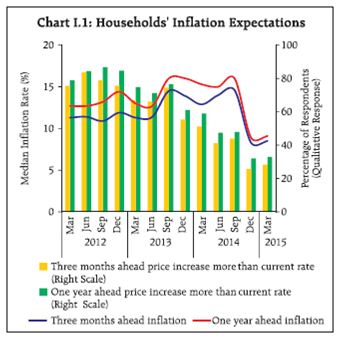
Inflation expectations of various economic agents
polled in forward looking surveys have been easing,
partly reflecting the adaptation of expectations to
the decline in inflation as well as growing credibility
around the Reserve Bank’s inflation targets. Although
households’ expectations of inflation three months
ahead as well as one year ahead appear to have firmed
up modestly in March 2015 in response to the uptick
in retail inflation in January – February 2015, the
softening of food and fuel inflation will likely temper
those expectations going forward (Chart I.1 and
Box I.1). This is borne out by the survey of professional forecasters for March 2015 in which five years ahead
inflation expectations have dropped by 50 basis points to 5.3 per cent. Professional forecasters expect
CPI inflation to average between 5.0 and 6.0 per cent
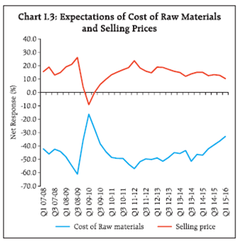
in 2015-16 (Chart I.2). The industrial outlook survey of the Reserve Bank indicates that manufacturers
expect softer input prices in the near-term, which
could transmit to output prices with a lag in view of
the slack in economic activity (Chart I.3).
 Box I.1: What is Driving Inflation Expectations?
Understanding the dynamic interaction between
inflation and inflation expectations is important for
setting monetary policy. Inflation is sensitive to change
in the output gap and inflation expectations, both of
which monetary policy can influence by modulating
aggregate demand. In countries where inflation
expectations are well anchored, inflation has become
less sensitive to variations in the output gap, leading to
a flattening of the Phillips curve. In these countries,
inflation has even become less sensitive to major supply
shocks (Bernanke, 2007).
Survey-based gauges of expectations tend to be
somewhat backward-looking for the near term –
responding to changes in actual inflation, Price
movements of frequently bought food products have a
significant bearing on inflation expectations. Fuel prices
also move inflation expectations quickly: despite having
lower weights in the consumption basket, their price
changes get wide publicity in the media and influence
expectations faster than their actual impact on the
consumption basket. Longer-term expectations are
typically more stable. Empirical analysis using data for
the period September 2008 to December 2014 shows
that 3 months ahead inflation expectations move largely
in response to changes in prices of vegetables/fruits and
petrol – which together explain almost 60 per cent of the change in inflation expectations. These findings are
robust, i.e., even if the last quarter (October-December
2014) – when inflation expectations declined sharply
– is excluded from the sample, the estimated coefficients
remain stable.
The experience of inflation targeting countries suggests
that a credible monetary policy framework with clarity
about the objective function of the central bank helps in
anchoring inflation expectations. In the UK for example,
just the announcement of instrument independence for
the Bank of England in May 1997 led to an immediate
fall in inflation expectations by 50 basis points along the
entire term structure (Haldane, 2000). In this context,
the Monetary Policy Framework Agreement in India
should be able to reinforce the disinflationary forces
currently at work and anchor inflation expectations
around the medium-term inflation target.
References:
Bernanke, Ben S. (2007), “Inflation Expectations and
Inflation Forecasting”, July 10, 2007. <http://www.federalreserve.gov/newsevents/speech/bernanke20070710a.htm>
Haldane, Andrew (2000) “Targeting Inflation: The United
Kingdom in Retrospect”, <https://www.imf.org/external/pubs/ft/seminar/2000/targets/strach7.pdf>
I.1 Outlook for Inflation
Turning to inflation forecasts, large and unanticipated
changes in initial conditions referred earlier warrant
revised baseline assumptions (Table I.1). Updated
estimates of structural models and information yielded
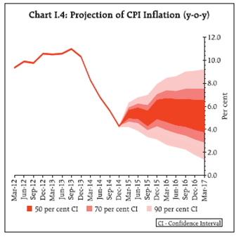
by surveys and market-based gauges indicate that CPI
inflation will remain below the target of 6 per cent set
for January 2016, hovering around 5 per cent in the
first half of 2015-16, and a little above 5.5 per cent in the second half (Chart I.4). Uncertainties surrounding
commodity prices, monsoon and weather-related
disturbances, volatility in prices of seasonal items
and spillovers from external developments through
exchange rate and asset price channels are reflected
in a 70 per cent confidence interval of 3.7 per cent to
7.9 per cent around the baseline inflation projection of 5.8 per cent for Q4 of 2015-16. Medium-term
projections derived from model estimates assuming
an unchanged economic structure, fiscal consolidation
in line with the recalibrated path, a normal monsoon
and no major exogenous or policy shocks indicate that
CPI inflation in 2016-17 could be around 5.0 per cent
in Q4 of 2016-17, with risks evenly balanced around it.
| Table I.1: Baseline Assumptions for Near-Term Projections |
| September 2014 MPR |
Current Assumptions |
• Indian crude oil basket price at US$ 100 per barrel for the remaining part of the year.
• Exchange rate at about Rs. 60 per US$ for the remaining part of the year.
• No increase in diesel prices from September 2014 onwards.
• No increase in administered liquefied petroleum gas (LPG) and kerosene prices in the remaining part of the year.
• Global growth picking up in the second half of the year, as projected in the World Economic Outlook (WEO) July 2014 update, IMF.
• Achievement of fiscal deficit targets as outlined in the Union Budget for 2014-15.
• No major change in domestic macroeconomic/structural policies during the forecast horizon. |
• Indian crude oil basket* price at US$ 60 per barrel in the first half and US$ 63 per barrel in the second half of FY 2015-16.
• Current level of the exchange rate.**
• No change in LPG and kerosene prices.
• Normal monsoons during 2015-16.
• Global economy expected to grow at 3.5 per cent in 2015 (weaker by 0.3 percentage point from earlier projections) as per the WEO January 2015 update, IMF.
• Achievement of fiscal deficit targets as indicated in the Union Budget for 2015-16.
• No major change in domestic macroeconomic/structural policies during the forecast horizon. |
* The Indian basket of crude oil represents a derived basket comprising
sour grade (Oman and Dubai average) and sweet grade (brent) crude oil
processed in Indian refineries in the ratio of 72.04:27.96 during 2013-14.
**The exchange rate path assumed here is for the purpose of generating
staff’s baseline growth and inflation projections and does not indicate any ‘view’ on the level of the exchange rate. The Reserve Bank is guided by the
need to contain volatility in the foreign exchange market and not by any
specific level/ band around the exchange rate.
|
 I.2 Outlook for Growth
Real Gross Domestic Product (GDP) growth for 2014-
15 was projected by the Reserve Bank at 5.5 per
cent. The CSO’s provisional estimates of GDP (base:
2004-05) tracked staff’s projected path well up to Q2
of 2014-15. The new GDP data (rebased to 2011-12)
released by the Central Statistics Office (CSO) at the
end of January 2015 and on February 9, however,
came as a major surprise as it produced significantly
higher growth at constant prices. The divergence
between the new series and the old series in the pace
of growth of the manufacturing sector has turned
out to be stark; in particular, the robust expansion
of manufacturing portrayed in the new series is not
validated by subdued corporate sector performance
in Q3 and still weak industrial production5. In the
financial and real estate sub-sector, the high growth of
13.7 per cent at constant prices is not corroborated by
the observed sluggishness in key underlying variables
such as credit and deposit growth, housing prices,
rent and most importantly, the subdued performance of real estate companies in terms of sales growth and
earnings. Data revisions and their after-effects are
not unique to India, but the magnitude of the gap in
real GDP growth rates between the old and the new
series for 2013-14 and 2014-15 has complicated the
setting of monetary policy. Undoubtedly, the new
GDP data embody better coverage and improved
methodology as per international best practices. Yet
these data cloud an accurate assessment of the state
of the business cycle and the appropriate monetary
policy stance; particularly, they render forecasting
tenuous. Projections based on the new series are also
handicapped by the lack of sufficient history in terms
of backdated data amenable to modelling.
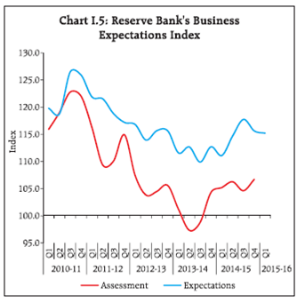 The macroeconomic environment is expected to
improve in 2015-16, with fiscal policy gearing to an
investment-led growth strategy6 and monetary policy
using available room for accommodation. Business
conditions in Indian manufacturing assessed in
the Reserve Bank’s Business Expectations Index
(BEI) developed from its industrial outlook survey
indicates that Q1 of 2015-16 may see some tempering
of the improvement in the second half of 2014-15
(Chart I.5). This is corroborated by some of the surveys
polled by other agencies (Table I.2). It is important to recognise though that most of these surveys were
conducted before the presentation of the Union
Budget and the easing of monetary policy on March
4. The Reserve Bank’s consumer confidence survey (CCS) points to growing consumer optimism since
June 2014, reflecting purchasing power gains arising
from lower inflation as well as improved perception of
income, spending and employment growth (Chart I.6).
| Table I.2: Business Expectations Surveys |
| |
NCAER
Business
Confidence
Index
Q4: 2014-15 |
FICCI
Overall
Business
Confidence
Index
February 2015 |
Dun and
Bradstreet
Business
Optimism
Index
Q1: 2015 |
CII Business
Confidence
Index
Q3: 2014-15 |
| Current level of the index |
148.4 |
70.5 |
129.4 |
56.4 |
| Index as per previous survey |
142.5 |
70.4 |
137.6 |
56.2 |
| Index levels one year back |
122.3 |
60.8 |
157.2 |
49.9 |
| % change (q-o-q) sequential |
4.1 |
0.1 |
-6.0 |
0.4 |
| % change (y-o-y) |
21.3 |
16.0 |
-17.7 |
13.0 |
Large declines in commodity prices and the benign
inflation outlook for the near-term should provide a
boost to growth (Box I.2).
Nevertheless, there are downside risks to growth
which could restrain growth prospects if they
materialise. The ongoing downturn in the international
commodity price cycle, which commenced in 2012, could reverse, given occasional signs of oil prices
reviving ahead of global economic activity. In fact,
the volatile geopolitical environment could even
hasten the reversal. The consequent resurgence of
inflation pressures could overwhelm the nascent
conditions setting in for recovery. Risks to budgetary
forecasts from tax shortfalls, subsidy overshoots and
disinvestment under-realisation could impact the
level of budgeted allocation for capital expenditure.
Early warnings on the south-west monsoon,
given the probability of about 50 per cent
currently being assigned to an El Nino event,
could dent the outlook for agriculture. Finally, if
the decline in the gross saving as percentage of
Gross National Disposable Income (GNDI) from
33 per cent in 2011-12 to 30 per cent in 2013-14
continues into the medium-term, it could tighten
the financial constraint to growth unless productivity
improves significantly.
Box I.2: Decline in Oil Prices – Impact on Growth and Inflation
For a large net importer of crude oil like India, the decline
in crude prices since June 2014 by about 50 per cent is
a favourable external shock. Going forward, this could
work towards improving growth prospects and easing
inflation pressures further. Crude prices could impact
economic activity and inflation in India through several
channels: (i) higher real incomes for consumers; (ii)
lower input costs, boosting corporate profitability and
inducing investment; (iii) lower current account deficit
(CAD); and (iv) improved market sentiment. These
favourable effects could, however, be offset by weak
global demand.
In India, a US$ 50 per barrel decline in oil prices (Indian
basket) sustained over one year could give rise to higher
real income equivalent of about 4 per cent of total private
consumption demand and about 2.9 per cent of nominal
GDP. Assuming 50 per cent pass-through to domestic
prices of petroleum products, the real income gain could
enhance aggregate consumption demand by about 2 per
cent and output by more than 1 per cent. For the
corporate sector in India, particularly non-oil producing
firms (such as cement, electricity, iron and steel, chemicals, textiles and transportation), with more than
5 per cent of their total costs in the form of fuel, panel
regressions show a statistically significant inverse
relationship between profitability and oil prices. Model
estimates suggest that for a 10 per cent decline in oil
prices (under alternative assumptions of pass-through
to CPI) output growth could improve in the range of
0.1-0.3 percentage points, while CPI inflation could
decline by about 20-25 basis points below the baseline.
A caveat is in order though. The estimates presented
under the balance of risks in this Chapter may differ due
to different dynamics captured in different models and
varying assumptions on pass-through. For instance in
India, the entire decline in crude prices was not fully
passed on because of the increase in excise duty on
petroleum products by the Government. This suggests
that model-based estimates at best could be indicative
rather than precise.
Reference:
World Bank (2015). “Global Economic Prospects”, January
2015.
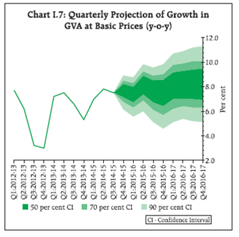
Growth projections combining these forward looking
assessments and model-based forecasts, including
time series forecasts such as autoregressive integrated
moving average (ARIMA) and Bayesian vector auto
regressions (BVAR), point to a gradual pick-up in
growth. Quarterly projections relate to gross value
added (GVA) at basic prices, because of more robust
estimation relative to expenditure side GDP and also
due to better clarity on key indicators that are used
in the compilation of data by the CSO. Growth in
GVA at basic prices for 2015-16 is projected at 7.8 per
cent, with risks evenly balanced around this baseline
forecast. Possible revision to CSO’s estimates for
2014-15 is a key risk to the forecast, with the revisions
expected to be in the downward direction (please
see Chapter III) and consequently an upside bias gets
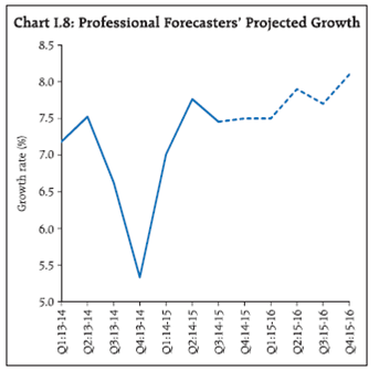
built in (Chart I.7)7. For 2016-17, real growth in GVA
at basic prices is projected at 8.1 per cent, assuming
gradual cyclical recovery on the back of a supportive
policy environment, but without any policy induced
structural change or any major supply shock. If the
GDP growth for 2014-15 is revised down by the CSO,
the trajectory will change accordingly. The Reserve
Bank’s professional forecasters’ survey indicates an average GVA growth of 7.9 per cent for 2015-16 (Chart
I.8 and Table I.3).
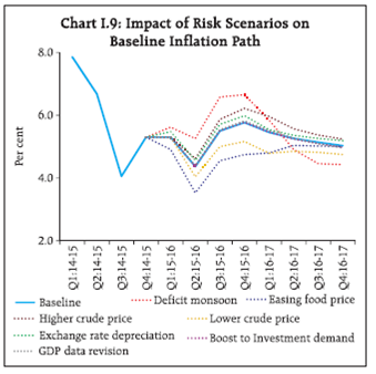
 I.3 Balance of Risks
The baseline paths projected for growth and inflation
are subject to realisation of a set of underlying
assumptions (Table I.1). The likely paths relative to
the baseline that may evolve under plausible risk
scenarios are set out below (Charts I.9 and I.10).
(a) Sharp Increase in Crude Oil Prices
Global crude oil prices are assumed to increase
gradually over the forecast horizon in the baseline
projections. There is, however, a non-trivial risk of a sharp increase in international crude prices triggered
by the materialisation of geo-political tensions and
other supply disruptions. In the event of such a shock pushing crude oil prices up by about US$ 15-20 per
barrel above the baseline, inflation could be higher
by about 40-60 basis points (bps) by the end of 2015-16 (on account of both direct and indirect effects).
Growth could weaken by 10-30 bps over the next two
years as the direct impact of higher input costs would
be reinforced by spillover effects from lower world
demand.

| Table I.3: Reserve Bank's Baseline and Professional Forecasters' Median Projections |
| Reserve Bank’s Baseline |
2014-15 |
2015-16 |
2016-17 |
| Inflation (Y-o-Y) in Q4 |
5.3 |
5.8 |
5.0 |
| Output Growth (per cent) – GVA at basic prices |
7.5 |
7.8 |
8.1 |
| Fiscal Deficit (per cent of GDP) |
4.1 |
3.9 |
3.5 |
| Current Account Balance (per cent of GDP) |
-1.3 |
|
|
| Assessment of Survey of Professional Forecasters |
| Key Macroeconomic Indicators* |
2014-15 |
2015-16 |
|
| Growth rate of GVA at basic prices at constant prices (2011-12) (per cent) |
7.5 |
7.9 |
|
| Agriculture & Allied Activities |
1.1 |
3.4 |
|
| Industry |
5.9 |
6.3 |
|
| Services |
10.6 |
10.1 |
|
| Private Final Consumption Expenditure growth rate at current prices (per cent) |
12.9 |
13.0 |
|
| Gross Saving (per cent to Gross National Disposable Income) |
30.0 |
31.0 |
|
| Gross Fixed Capital Formation (per cent of GDP) |
28.6 |
29.3 |
|
| Money Supply (M3) (growth rate in per cent) (end period) |
12.3 |
13.5 |
|
| Bank Credit of all scheduled commercial banks (growth rate in per cent) |
12.0 |
14.0 |
|
| Combined Gross Fiscal Deficit (per cent to GDP) |
6.5 |
6.3 |
|
| Central Govt. Fiscal Deficit (per cent to GDP) |
4.1 |
3.9 |
|
| Repo Rate (end-period) |
7.50 |
7.00 |
|
| CRR (end-period) |
4.00 |
4.00 |
|
| T-Bill 91 days Yield (end-period) |
8.2 |
7.5 |
|
| YTM of Central Govt. Securities 10-years (end-period) |
7.8 |
7.3 |
|
| Overall Balance of Payments (US $ bn.) |
49.6 |
49.4 |
|
| Merchandise Exports (US $ bn.) |
323.5 |
339.9 |
|
| Merchandise Exports (growth rate in per cent) |
2.0 |
3.4 |
|
| Merchandise Imports (US $ bn.) |
466.7 |
478.2 |
|
| Merchandise Imports (growth rate in per cent) |
0.3 |
2.0 |
|
| Trade Balance as per cent of GDP at current prices |
-6.9 |
-6.3 |
|
| Net Invisibles Balance (US $ bn.) |
115.8 |
119.2 |
|
| Current Account Balance (US $ bn.) |
-25.0 |
-20.0 |
|
| Current Account Balance as per cent to GDP at current prices |
-1.2 |
-1.0 |
|
| Capital Account Balance (US $ bn.) |
76.3 |
66.5 |
|
| Capital Account Balance as per cent to GDP at current prices |
3.5 |
2.9 |
|
Source: 33rd Round of Survey of Professional Forecasters (March 2015).
* : Median of forecasts. |
(b) Below Normal Monsoon in 2015-16
As against the normal monsoon assumption in the
baseline, there is a risk of monsoon turning out to be
deficient in 2015. This could lead to a lower agriculture
output which, in turn, would lower the overall GVA
growth by around 40 bps in 2015-16. Food prices could
consequently increase, leading to inflation rising
above the baseline by 80-100 bps in 2015-16. Factors
like spatial and temporal distribution of monsoon,
policies relating to food stocks, procurement and
minimum support prices (MSPs) may moderate or
accentuate the impact of rainfall deficiency.
(c) Depreciation of the Rupee
Uncertainties surrounding the exchange rate persist.
The key risk is that normalisation of monetary
policy by the US Fed which may spark off safe haven
capital flows into US treasuries and spur further
appreciation of the US dollar. On the other hand,
deflation risks in some of the advanced economies
could warrant further monetary accommodation.
A depreciation of the rupee by around 10 per cent,
relative to the baseline assumption of the current
level of exchange rates continuing, could raise
inflation by around 20 -30 bps in 2015-16. On average,
growth would be higher by about 10 bps in 2015-16
due to an improvement in the external trade balance
while it could turn out to be marginally weaker in
2016-17, assuming tightness in financial conditions
intensifying further on materialisation of risks in
the external environment.
(d) Easing of Food Inflation
Headline inflation could also undershoot from the
baseline if food inflation moderates by more than what
is envisaged. This could be brought about by positive
supply shocks, especially through improvements in
the supply chain, reforms in market infrastructure
and a step-up in investment in agriculture. In such a
scenario, headline inflation may be lower by around
100 bps than the baseline by the end of 2015-16.
(e) Crude Oil Price Declining Further
If crude oil prices decline below the baseline by
US$ 15-20 per barrel in the near-term as a result of
excess supply conditions/low global demand in a
stable geo-political environment, inflation could turn
out to be 30-60 bps below the baseline by the end of
2015-16. Such a decline in crude prices would also
raise GVA growth by 10-30 bps above the baseline in
the next two years under different pass-through
scenarios.
(f) Revision in CSO’s GDP Estimates
Considerable uncertainty surrounds the advance
estimates of GDP growth for 2014-15 and information
on real economic activity relating to Q4 is expected to
be better captured in the revised estimates, which
would be released around the end of May 2015. If GVA
growth (at constant prices) gets revised downwards by
50 bps in the subsequent release(s), it would alter the
assessment of demand conditions and a decline in the
inflation trajectory for the medium-term by 10-30 bps
could result.
(g) Pick-up in Investment Demand
If the boost to investment expenditure announced in
the Union Budget for 2015-16 helps in crowding in
private investment, and correspondingly, if
investment demand picks up, GDP growth may turn
out to be over 50 bps above the baseline in 2015-16.
With augmentation of capacity but a still negative
output gap, the impact of higher investment demand
on inflation in 2015-16 could be minimal.
The balance of risks and possible deviations of
inflation and growth paths from their projected
baselines warrant a careful appraisal of forward
guidance, especially the underlying conditions that
drive such guidance (Box I.3).
The outlook for growth and inflation is informed by
the assessment of macroeconomic and financial
conditions presented in Chapters II to V. Barring
unforeseen shocks, the near-term appears to be
characterised by continuing slack in the economy.
Fiscal consolidation intentions and weak rural
consumption demand are likely to keep demand side
risks to inflation contained. From the supply side,
risks in the form of reversal in global commodity
prices, uncertainty surrounding monsoon outcomes,
and possible exchange market pressures arising from volatility in capital flows associated with US monetary
policy normalisation would need to be monitored
carefully and continuously, given the past experience
with spillovers from taper talk. The room for accommodating supply shocks in the conduct of
monetary policy remains limited, even as supporting
the revival of investment demand assumes high
importance.
Box I.3: Forward Guidance under Uncertainty
Forward guidance acquired prominence in the
communication of monetary policy of central banks
of both advanced and emerging economies after the
global crisis, particularly on confronting the zero
lower bound (ZLB) constraint. Traditionally, forward
guidance before the global crisis used to be in the form
of “forecast but do not promise”; but at ZLB it became
a policy instrument – investment demand could be
conditioned by expectations about the future path
of short-term interest rates. Thus, forward guidance
at ZLB potentially amplified the easing impact of
unconventional monetary policy.
The use of forward guidance as an instrument of policy
in normal times shifts the burden of understanding
risks and uncertainty primarily to central banks who,
in turn, face the trade-off between “credibility” and
“flexibility”. Four broad variants of forward guidance
have been used by central banks in the post-crisis
period: (a) qualitative guidance on the likely stance
of policy without linking it to any explicit end date,
threshold value of any goal variable or key parameters;
(b) qualitative guidance linked to evolution of specific
state variables; (c) calendar-based forward guidance
specifying the exact period over which the same
policy stance will prevail; and (d) outcome-based
forward guidance linked to threshold values of state
variables. While the first two variants are somewhat
open-ended, the third is time-contingent and the last
one is state-contingent. Time and state-contingent
forward guidance provides greater certainty, but strong
commitment may limit flexibility. Balance of risks
assessments often assume specific identifiable risks
and the manner in which these could be transmitted.
Unanticipated risks and model errors, however, could make the evolution of inflation and growth paths
quite different from either the baseline or the risk
scenarios. Financial market frictions could complicate
risk assessment further, especially if they are either
not explicitly modelled or their dynamic interactions
with the real economy are not captured properly in
models. When benefits of commitment under forward
guidance are assessed against benefits of changing the
policy stance not fully consistent with the guidance,
occasionally the latter may be preferred because of
developments that were hard to anticipate at the time
of giving the forward guidance. This has led to the
view that forward guidance should be a tool that must
be reserved for use only under the ZLB constraint:
“...For the policy practitioner, uncertainty is not abstract,
it is a daily preoccupation. Uncertainty and the policy
errors it can foster must not only be embedded in our
decision-making processes ex ante, they must be worn
like an ill-fitting suit ex post, that is, with humility”
(Poloz, 2014).
In India, forward guidance has served the purpose of
guiding market expectations around monitoring the
sources of and risks to inflation. Given the uncertainties
surrounding time varying output gap estimates, the
evolution of exogenous factors driving the inflation
process, global spillovers, and the nature, size and
timing of measures undertaken by the Government
to contain inflation, forward guidance has to be
conditioned by incoming data.
Reference:
Poloz, Stephen S. (2014). “Integrating Uncertainty and
Monetary Policy-Making: A Practitioner’s Perspective”,
Bank of Canada Discussion Paper 2014-6.
II. Prices and Costs
The trajectory of headline inflation in the second half of 2014-15 turned out to be substantially lower than staff ’s
assessment set out in the MPR of September 2014, aided by a sharp fall in global commodity prices and domestic
food inflation. Cost pressures eased with falling raw material prices and slowdown in wage growth.
Three major developments that followed the first
Monetary Policy Report (MPR) of September 2014 have
dramatically altered the evolution of underlying price/
cost conditions. First, the pass-through of the 28 per
cent plunge in international commodity prices1 into
domestic food, fuel and services prices worked in
conjunction with the disinflationary stance of monetary
policy to bring down inflation to 5.4 per cent in February
2015. Second, the Central Statistics Office (CSO)
unveiled data revisions relating to consumer price
index (CPI) and national accounts in January-February
2015 that updated the base years/weighting schemes
and also brought in methodological improvements to align with international best practices (Boxes II.1 and
III.1). Going forward, these information upgrades will
have a bearing on staff’s assessment of inflation
formation and forecasts. Third, the Government of
India and the Reserve Bank formalised a landmark
agreement on the monetary policy framework alluded
to in Chapter I.
These institutional changes will condition the future
path of inflation to which the Reserve Bank and the
Government of India are committing, if fiscal targets
are adhered to and administrative interventions in the
formation of key prices, wages and interest rates are
minimised.
Box II.1: Revision of the Consumer Price Index (CPI)
Beginning January 2015, the CSO revised the base year
of the CPI to 2012 (from 2010=100). The weighting
pattern of the revised series is based on the 2011-
12 Consumer Expenditure Survey (CES) of the
National Sample Survey Office (NSSO), which is more
representative and recent than the CES 2004-05 used
for the old series (Table II.B.1). A number of
methodological improvements have also been
undertaken by the CSO in the new series, which
include:
i. weighting diagrams use the modified mixed
reference period* (MMRP) data of CES 2011-12 as
against a uniform reference period (URP) of 30 days
used in the earlier series;
ii. geometric mean of the price relatives with respect
to base prices is used to compile elementary/item
indices, instead of the arithmetic mean used in
the old series, thereby reducing the impact of large
discrete change in prices over different markets;
iii. in case of items sold through the public distribution
system (PDS), prices of items covered under the
antyodaya anna yojana (AAY) have also been included in addition to those items covered by
above poverty line (APL) and below poverty line
(BPL) categories; and
iv. the sample size for collection of house rent data has
been doubled from 6,684 in the old series to 13,368
in the revised series.
| Table II.B.1: Comparison of Weighting Diagrams–Previous and Revised CPI |
| (Per cent) |
| |
Rural |
Urban |
Combined |
| 2010
Base |
2012 Base |
2010
Base |
2012
Base |
2010
Base |
2012
Base |
| Food and beverages |
56.59 |
54.18 |
35.81 |
36.29 |
47.58 |
45.86 |
| Pan, tobacco and intoxicants |
2.72 |
3.26 |
1.34 |
1.36 |
2.13 |
2.38 |
| Clothing and footwear |
5.36 |
7.36 |
3.91 |
5.57 |
4.73 |
6.53 |
| Housing |
-- |
-- |
22.54 |
21.67 |
9.77 |
10.07 |
| Fuel and light |
10.42 |
7.94 |
8.40 |
5.58 |
9.49 |
6.84 |
| Miscellaneous |
24.91 |
27.26 |
28.00 |
29.53 |
26.31 |
28.32 |
| Total |
100 |
100 |
100 |
100 |
100 |
100 |
| Excluding Food and Fuel |
32.99 |
37.88 |
55.79 |
58.13 |
42.93 |
47.30 |
*Under MMRP, data on expenditure incurred are collected for frequently
purchased items – edible oil, eggs, fish, meat, vegetables, fruits, spices, beverages,
processed foods, pan, tobacco and intoxicants – during the last seven days; for
clothing, bedding, footwear, education, medical (institutional), durable goods,
during the last 365 days; and for all other food, fuel and light, miscellaneous goods
and services including non-institutional medical services; rents and taxes during
the last 30 days. |
II.1. Consumer Prices
The MPR of September 2014 had noted that the
receding of inflationary pressures, guided by the
monetary policy stance set out in January 2014, halted
in the first half of 2014-15. While fuel inflation and
inflation excluding food and fuel underwent steady
moderation, headline inflation was propped up by food
inflation, which experienced bouts of weather-induced
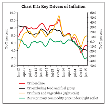
short-lived surges. In September, however, inflation
eased by 140 basis points. From September to
November, disinflation gathered momentum and
turned out to be faster than initially anticipated under
the combined influence of a large decline in global
commodity prices, softening of prices of fruits and
vegetables domestically, continuing slack in the
economy and the favourable ‘base effect’ of higher
inflation a year ago (Chart II.1).
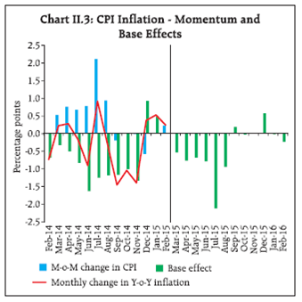
 The role of this base effect in inflation outcomes during
2014-15 turned out to be non-trivial. Just as it shaped
the rapid disinflation until November, its reversal from
December produced an upturn, despite still benign
international commodity prices and moderate domestic
food and input prices. Sequential changes in headline
inflation reflect the combined impact of month-on-month
(m-o-m) changes in prices – which provide an
indication of the speed at which prices are evolving –
and base effects. The momentum of headline inflation
has been weak through December-February, mostly due
to the prices of non-durable goods, especially perishable
food (Chart II.2a). M-o-M price changes embodied in a diffusion index also point to weak momemtum;
however, broad-based price pressures persist across
items within the CPI (Chart II.2b). Going forward, base
effects are likely to exert a downward pull on headline
inflation up to August 2015 (Chart II.3).
II.2 Drivers of Inflation
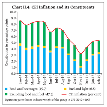
The intra-year path of headline inflation in 2014-15
exhibited higher volatility than in past years,
essentially reflecting the contributions of its
constituents (Chart II.4). The contribution of the food
category weighted by its share in the CPI underwent
large variations – accounting for more than half of
headline inflation in the first half of 2014-15, but declining to about a third in November before
increasing to close to 60 per cent by February. By
contrast, the contribution of the category excluding
food and fuel has been relatively stable, with some
decline in recent months.
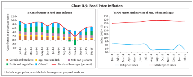
 Within the food group, different drivers have propelled
individual elements (Chart II.5a). For cereals, moderation
in inflation is attributable to lower increases in MSPs
in 2014-152, active supply management policies in the
form of increased allocation under the public
distribution system (PDS) as well as open market sales
of wheat. Moreover, an index of prices of PDS items (rice, wheat and sugar) captured within the CPI shows
that PDS prices have fallen significantly even as market
prices of these items have risen (Chart II.5b). In the
case of vegetables and fruits, prices declined faster than
expected in response to policy actions to discourage
stockpiling3. Sugar prices moderated in consonance
with global prices. However, prices of protein-rich items
(eggs, fish, meat, milk and pulses) exhibited downward
rigidity, reflecting structural mismatches between
demand and supply.
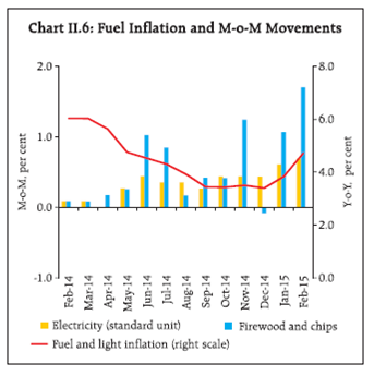
 In the absence of revisions in administered prices of
coal and cooking gas, fuel group inflation declined during the year, but rose to 4.7 per cent in February,
mainly on account of increase in firewood and
electricity prices (Chart II.6). The still large under-recovery
on account of kerosene and cooking gas
impeded the pass-through of lower international prices
to administered prices of these items. During April-
December 2014, under-recoveries of oil marketing
companies (OMCs) in respect of sale of kerosene and
cooking gas accumulated to `562 billion, amounting to
potential outgoes under subsidies in spite of the drastic
fall in international prices.
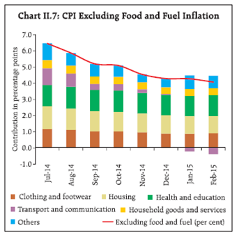
 With the pass-through of monetary policy actions into
the economy, inflation excluding food and fuel ebbed
steadily during 2014-15, reaching 4.1 per cent in
February (Chart II.7). The decline in housing inflation
(rentals) has been pronounced in the new base series
relative to the old series in part due to methodological
improvements set out in Box II.1. Inflation in prices of
services such as health, education and household
services showed some moderation in recent months,
reflecting the slowdown in wage growth.
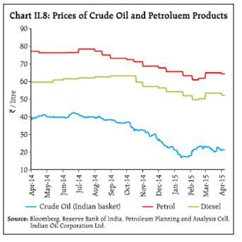
 For the transport and communication sub-group,
deflation has set in from January 2015 under the impact
of a sharp decline in international crude oil prices
which affected prices of fuels included in this subgroup.
Between June 2014 and January 2015, crude oil
prices (Indian basket, rupee terms) declined by around
55 per cent, with 90 per cent of this fall occurring during
October to January. In response, retail prices of petrol softened. Diesel prices, on the other hand, were
increased step-wise till August in order to eliminate
under-recoveries of OMCs; thereafter, there was a
reduction during October to January (Chart II.8). The
decline in domestic pump prices, however, was much
lower than the downward movement in international
crude oil prices on account of increases in excise duty
cumulatively by `7.75 per litre on petrol and by `6.50
on diesel starting November 2014. Global crude prices
remained volatile during February-March, tracking
geopolitical and other global supply side developments
referred to earlier.
 Other Measures of Inflation
All measures of inflation generally co-moved with the
headline CPI inflation since the last MPR. The decline
in inflation in terms of the wholesale price index (WPI),
however, has been most significant with a contraction
of 2.1 per cent in the month of February 2015
(Table II.1).
II.3 Costs
Since the MPR of September 2014, cost-push pressures
in the Indian economy have eased significantly. As
shown in the foregoing section, external cost conditions
associated with imports of commodities, particularly
crude and petroleum products, have declined on a large
scale. This is directly reflected in the drop in wholesale
price inflation into negative territory. Domestically too,
input cost pressures have been abating on a sustained
basis since June. However, the existence of supply
constraints in various sectors of the economy is
impeding a fuller response of output prices to these
developments.
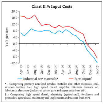
Input costs for both farm and industrial sectors have
contracted since Q3 of 2014-15 (Chart II.9).
Manufacturing firms participating in the Reserve Bank’s
industrial outlook survey also indicated sizable declines
in raw material costs, with the lowest cost pressures
since the January-March 2010 round (Table II.2). They
have also been reporting improvement in pass-through
into selling prices, including in the January-March 2015
round. Purchasing managers’ surveys for both
manufacturing and services corroborate these
assessments – the narrowing of the gap between input and output prices is indicating weakening pricing
power.
| Table II.1: Measures of Inflation |
| (Y-o-Y, per cent) |
| Quarter/
Month |
GDP
deflator |
WPI |
CPI |
CPI-
IW |
CPI-
AL |
CPI-
RL |
| Q1: 2013-14 |
5.3 |
4.8 |
9.5 |
10.7 |
12.6 |
12.4 |
| Q2: 2013-14 |
6.7 |
6.6 |
9.7 |
10.8 |
12.9 |
12.7 |
| Q3: 2013-14 |
7.9 |
7.1 |
10.4 |
10.6 |
12.4 |
12.3 |
| Q4: 2013-14 |
5.1 |
5.4 |
8.2 |
6.9 |
8.5 |
8.7 |
| Q1: 2014-15 |
5.9 |
5.8 |
7.8 |
6.9 |
8.1 |
8.3 |
| Q2: 2014-15 |
4.3 |
3.9 |
6.7 |
6.8 |
7.3 |
7.6 |
| Q3: 2014-15 |
1.4 |
0.3 |
4.1 |
5.0 |
5.4 |
5.7 |
| Jan-15 |
-- |
-0.4 |
5.2 |
7.2 |
6.2 |
6.5 |
| Feb-15 |
-- |
-2.1 |
5.4 |
6.3 |
6.1 |
6.2 |
| IW: Industrial Workers, AL: Agricultural Labourers and RL: Rural Labourers. |
 Wage growth, another key determinant of costs, has
been decelerating, albeit from high levels, across
various sectors of the economy in recent years. The
slowdown in rural wage growth has been particularly
noteworthy. The Labour Bureau revised data on rural
wages in November 2013 to incorporate a number of
new occupations besides reclassification of the existing
occupations. It estimates that average annual growth
in rural wages was 5.5 per cent for all occupations
(agricultural and non-agricultural) for male workers in
January 2015, substantially lower than the annual
average growth of 15 per cent during the six-year period
(2007-13) reported in the old series (Chart II.10). The
slowdown in wage growth has been more pronounced in the case of unskilled labourers, presumably reflecting
catch-up of low-wage states, sustained decline in rural
inflation and emphasis towards productive asset
creation relative to employment in public schemes such
as under the Mahatma Gandhi National Rural
Employment Guarantee Act (MGNREGA). These
developments suggest that high real wage growth
without commensurate improvements in productivity
is not sustainable.
| Table II.2: Input Costs and Selling Prices |
| (Net response in per cent) |
| |
Total Response
(Number) |
Cost of Raw
Materials |
Selling Prices |
| Jan-Mar 13 |
1301 |
-53.5 |
9.1 |
| Apr-Jun 13 |
1321 |
-49.9 |
7.3 |
| Jul-Sep 13 |
1207 |
-62.2 |
11.3 |
| Oct-Dec 13 |
1223 |
-55.3 |
7.8 |
| Jan-Mar 14 |
1114 |
-54.1 |
9.6 |
| Apr-Jun 14 |
1293 |
-49.5 |
9.8 |
| Jul-Sep 14 |
1225 |
-44.7 |
6.8 |
| Oct- Dec 14 |
2083 |
-41.5 |
5.9 |
| Jan-Mar 15 |
1533 |
-32.8 |
2.6 |
| Source: Industrial Outlook Survey, RBI. |
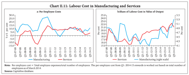
Unit labour costs4 in manufacturing and services have
picked up recently after moderating since 2013 (Chart II.11a). There was also a rise in the share of
labour cost in total output, especially for the
manufacturing sector (Chart II.11b).
The State of Aggregate Supply
Assessments of price/cost conditions in the economy,
juxtaposed with the results of empirical analysis,
provide useful insights into the state of aggregate
supply – the responsiveness of aggregate output to price
changes. Several factors determine the behaviour of
aggregate supply, including the time-varying price-setting
behaviour of firms in response to changes in
marginal cost; the nature of price-setting, whether
backward-looking or more flexible; the way inflation
expectations are formed; and random supply shocks5.
In technical terms, while price-setting behaviour
determines the slope of the aggregate supply curve, the
formation of inflation expectations and the incidence
of supply shocks can produce shifts in the aggregate
supply curve.
 The empirical evidence suggests that the behaviour of
aggregate supply has been changing in recent years even
as inflation dynamics have been evolving into uncharted
territory. Price-setting behaviour of firms is now
reckoned as less backward-looking than before; also,
the response of inflation to demand and supply shocks
has declined. Internationally, this has led to a loose
consensus around the view that the aggregate supply
curve has flattened and is turning out to be less sensitive to price shocks6. What this implies in the
context of conducting monetary policy is that every
unit of disinflation is going to cost more in terms of
the sacrifice of output to rein in that amount of
inflation.
Empirical evidence available in the Indian context
suggests that the behaviour of aggregate supply has
undergone a change during the post-global crisis period
in a manner that is broadly consistent with the
international experience, but with country-specific
nuances. In particular, the responsiveness of retail
inflation to changes in marginal costs has declined.
Furthermore, the sacrifice ratio7 has increased markedly
relative to the international evidence. This has
implications for monetary policy: going forward, every unit of inflation lowered is going to mean larger output
foregone, and the state of the economy is going to weigh
on the choice. Every cloud has a silver lining though;
unlocking stalled investments, bridging gaps in the
availability of key inputs such as power, land,
infrastructure and human skill, and rebuilding
productivity and competitiveness will improve the
supply response and sustain the disinflation currently
underway. This scenario envisages monetary policy in
a steering rather than interventionist role in its
commitment to price stability as its primary objective.
Finally, as regards the impact of shocks, exchange rate
pass-through8 has declined significantly. On the other
hand, domestic shocks such as a deficient monsoon
leave progressively deeper imprints on retail inflation
and increase the persistence of inflation expectations.
III. Demand and Output
Domestic economic activity firmed up in 2014-15, spurred by a pick-up in manufacturing and services. Little
definitive evidence, however, is available on a clear ‘break-out’ of economic activity. Key macroeconomic indicators,
leading and coincident, point to the presence of considerable slack in the economy.
Recent upgrades to the national accounts by the CSO
indicate that a rebound in economic activity that
started in 2013-14 has gathered pace in the second
half of 2014-15. While these estimates have generated
considerable public scrutiny and debate, there is a
building optimism that an inflexion point in the
economic cycle is approaching. As inflation retreats in
an environment of macroeconomic and political
stability, confidence in setting a double-digit growth
trajectory for the Indian economy over the medium-term
is flooding back. Unleashing of these growth
impulses hinges around decisively cutting the Gordian
knot of binding supply constraints, investments
locked in stalled projects and shortfalls in the
availability of key inputs such as power, land,
infrastructure and human skill formation. Business
sentiment is also buoyed by investor-friendly tax
proposals, planned switches in public spending from
subsidies to investment that crowd in private
enterprise, structural reforms and the intention to
continue fiscal consolidation announced in the Union
Budget for 2015-16.
III. 1 Aggregate Demand
Advance estimates of the CSO indicate that the
growth of real GDP (market prices) picked up to 7.4 per cent in 2014-15 from 6.9 per cent a year ago
(Table III.1). Although official data for Q4 of 2014-15
will be available only by May 2015, implicit in
the advance estimates for the full year is a step-up in
the momentum of growth in the last quarter of the
year.
Driving this quickening of activity, the weighted
contribution of private final consumption expenditure
is estimated to have risen to 4.1 per cent in 2014-15
from 3.6 per cent in 2013-14. Quarterly data suggest,
however, that the growth of private final consumption
expenditure slowed down considerably in Q3 of
2014-15; it would need to have grown by around 12
per cent in Q4 to match advance estimates of 7.1 per
cent for the full year. Coincident and leading
indicators of consumption, however, point to
persisting fragility of private consumption demand.
Indicators of rural demand like sales of tractors and
two wheelers point to persisting weakness. Rural
income appears to have been adversely affected by
deficient monsoons and decelerating growth in rural
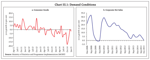
wages. Overall weakness in consumption demand is
also evident in the still depressed production of
consumer goods and significant deceleration in
corporate sales growth (Chart III.1).
| Table III.1: Real GDP Growth (Base:2011-12) |
| (Per cent) |
| Item |
Weighted Contribution to growth (Percentage points) |
2013-14 |
2014-15 (AE) |
2013-14 |
2014-15 |
| 2013-14* |
2014-15* (AE) |
Q1 |
Q2 |
Q3 |
Q4 |
Q1 |
Q2 |
Q3 |
| I. Private Final Consumption Expenditure |
3.6 |
4.1 |
6.2 |
7.1 |
7.7 |
5.6 |
4.6 |
7.0 |
4.3 |
8.7 |
3.5 |
| II. Government Final Consumption Expenditure |
0.9 |
1.1 |
8.2 |
10.0 |
27.3 |
5.3 |
11.0 |
-7.2 |
-2.0 |
5.8 |
31.7 |
| III. Gross Fixed Capital Formation |
0.9 |
1.3 |
3.0 |
4.1 |
2.3 |
6.3 |
5.3 |
-1.4 |
7.7 |
2.8 |
1.6 |
| IV. Net Exports |
4.4 |
0.4 |
69.0 |
19.5 |
25.6 |
55.8 |
90.0 |
91.0 |
68.7 |
-79.0 |
-115.4 |
| (i) Exports |
1.8 |
0.2 |
7.3 |
0.9 |
2.6 |
-1.6 |
15.7 |
14.1 |
9.3 |
-3.8 |
-2.8 |
| (ii) Imports |
-2.6 |
-0.1 |
-8.4 |
-0.5 |
-3.5 |
-8.4 |
-14.2 |
-7.0 |
-3.6 |
1.2 |
1.1 |
| V. GDP at Market Prices |
6.9 |
7.4 |
6.9 |
7.4 |
7.0 |
7.5 |
6.4 |
6.7 |
6.5 |
8.2 |
7.5 |
Note: AE: Advance estimates.
*Component-wise contributions do not add up to GDP growth in the table because change in stocks, valuables and
discrepancies are not included here.
Source: Central Statistics Office |
 Government final consumption expenditure (which
includes consumption expenditure of the centre,
states, local bodies and autonomous bodies) rose by
10 per cent in 2014-15 as per the advance estimates,
mainly on account of faster expenditure growth by
the states1. The aggregate expenditure growth of the
Centre, however, moderated. The increase in
expenditure on subsidies was offset by a sharp cutback
in plan revenue expenditure and aggregate capital
expenditure in order to adhere to the budgeted deficit
target. Austerity in respect of various categories of expenditure was also necessitated by the shortfall in
non-debt capital receipts and sluggish indirect tax
collections. Non-tax revenues, however, exceeded the
budgetary targets due to higher receipts on account of
dividends and profits (Table III.2). Disinvestment
receipts were less than half the budgeted amount in
2014-15.
| Table III.2: Key Fiscal Indicators - Central Government Finances |
| Indicators |
As per cent of GDP |
| 2014-15
(BE) |
2014-15
(RE) |
2015-16
(BE) |
| 1. Revenue Receipts |
9.2 |
8.9 |
8.1 |
| a. Tax Revenue (Net) |
7.6 |
7.2 |
6.5 |
| b. Non-Tax Revenue |
1.7 |
1.7 |
1.6 |
| 2. Total Receipts |
13.9 |
13.3 |
12.6 |
| 3. Non-Plan Expenditure |
9.5 |
9.6 |
9.3 |
| a. On Revenue Account |
8.7 |
8.9 |
8.5 |
| b. On Capital Account |
0.8 |
0.7 |
0.8 |
| 4. Plan Expenditure |
4.5 |
3.7 |
3.3 |
| a. On Revenue Account |
3.5 |
2.9 |
2.3 |
| b. On Capital Account |
0.9 |
0.8 |
1.0 |
| 5. Total Expenditure |
13.9 |
13.3 |
12.6 |
| 6. Fiscal Deficit |
4.1 |
4.1 |
3.9 |
| 7. Revenue Deficit |
2.9 |
2.9 |
2.8 |
| 8. Primary Deficit |
0.8 |
0.8 |
0.7 |
| BE : Budget estimates RE : Revised estimates
Source: Union Budget, 2015-16 |
The Union Budget 2015-16 has provided for higher
allocations to infrastructure and a substantial
increase in the resource transfer to states, keeping in
view the two-fold objectives of promoting inclusive
growth and strengthening fiscal federalism. This has
necessitated a deviation from the fiscal consolidation
trajectory in 2015-16 and an extension of the period of
convergence to the 3 per cent target for the gross fiscal
deficit (GFD) as a proportion to GDP by one year. The
budgeted reduction in GFD in 2015-16 reflects the
combined impact of a compression in plan revenue
expenditure and an increase in non-debt capital
receipts.
The CSO’s advance estimates of gradual pick-up in the
growth of gross fixed capital formation in 2014-15 do
not appear to be supported by its quarterly estimates
which indicate deceleration in Q2 and Q3 (Table III.1).
Although production of capital goods and non-oil nongold
imports gathered some momentum in Q4, a big
push in investment is essential for the economy to
break out of the vicious cycle of supply constraints,
stranded investments, stressed bank balance sheets,
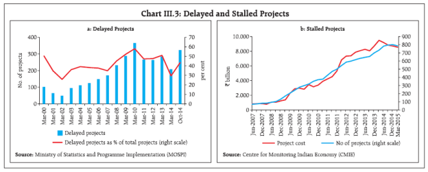
risk aversion and weak demand (Chart III.2). Progress
on speedier project clearances is, however, yet to
materalise (Chart III.3).
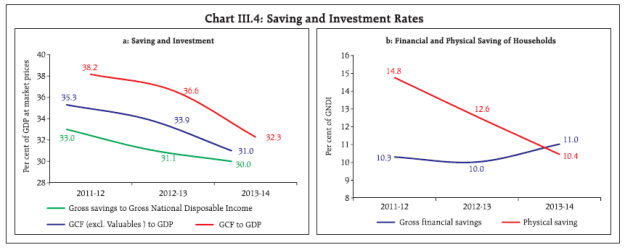
The gross domestic saving rate in the economy
has declined sharply over the last two years. The
decline was on account of lower savings in physical
assets by the household sector, mainly construction
(Chart III.4).
The contribution of net exports to overall GDP growth
turned negative since Q2 on contraction in exports
and some pick-up in imports. Exports shrank in Q3 on
weak global demand and the sharp fall in international
crude oil prices which affected exports of petroleum
products (POL) [accounting for around 19 per cent of
total merchandise exports]. Non-oil exports also
added to overall contraction as price realisation
declined considerably with the fall in international
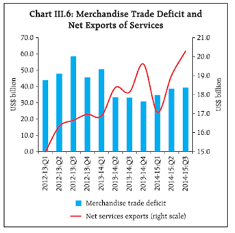
commodity prices (Chart III.5). With imports growing
at a modest pace, the trade deficit widened in Q3 of
2014-15, though it was partly offset by improved net
services exports (Chart III.6). During January and February 2015, the faster decline in imports relative to
exports significantly reduced the trade deficit. Net
services exports during January 2015 were, however,
lower than in the preceding month as well as a year
ago.
 In the financial account of India’s balance of payments,
capital flows remained strong during Q3. Though
equity flows weakened during the quarter, it was more
than offset by the large accretion under banking
capital as banks liquidated their overseas foreign
currency assets. In Q4, the improved investment
climate revived portfolio and foreign direct
investment, which dominated net capital flows.
Portfolio investment flows rose sharply to US$ 13.6
billion during Q4 from a relatively subdued level of
about US$ 6 billion in the preceding quarter. A surge
was evident in equity as well as debt investment by
foreign institutional investors (FIIs). Similarly, foreign direct investment rose to US$ 5.5 billion during
January 2015, more than twice the monthly average in
the preceding quarter. With net capital flows being
significantly larger than the external financing
requirement, foreign exchange reserves rose to a peak
level of US$ 343.0 billion by April 03, 2015.
 In terms of traditional metrics of foreign exchange
reserve adequacy – import cover and the Greenspan-
Guidotti rule for short-term debt cover – India has
exhibited steady improvement. The import cover of
reserves went up to 8.1 months at end-December 2014
from 7.8 months at end-March 2014 while the ratio of
short-term debt to reserves improved to 26.7 per cent
at end-December 2014 from 30.1 per cent at end-
March 2014 (Table III.3). Further, net forward purchases of US$ 5.6 billion and bilateral swap
arrangements with Japan and among the BRICS
provide additional cover against external shocks.
III.2 Output
The CSO’s new series of national accounts aligns with
internationally recognised best standards in terms of
the United Nations’ Systems of National Accounts
(SNA, 2008) and also improves data coverage. Output
measured by gross value added (GVA) at basic prices is,
however, in dissonance with various metrics tracked
as either coincident or leading indicators in terms of
both level and growth rates (Box III.1). In particular,
the conventional indicators of corporate performance
that are used to reflect movements in output and
Per cent which closely tracked the series in the old base, have
disconnected from the new series even after
accounting for the differences between the
‘establishment approach’ (old series) and ‘enterprise
approach’ (new series).
| Table III.3: External Sector Vulnerability Indicators |
| Indicator |
end-Mar
2001 |
end-Mar
2006 |
end-Mar
2011 |
end-Mar
2012 |
end-Mar
2013 |
end-Mar
2014 |
end-Dec
2014 |
| 1. External Debt to GDP ratio (%) |
22.5 |
16.8 |
18.2 |
20.9 |
22.3 |
23.7 |
23.2 |
| 2. Ratio of Short-term to Total Debt (Original Maturity) (%) |
3.6 |
14 |
20.4 |
21.7 |
23.6 |
20.5 |
18.5 |
| 3. Ratio of Short-term to Total Debt (residual maturity) (%) |
10.3 |
18.3 |
40.6 |
40.9 |
42.1 |
39.6 |
NA |
| 4. Ratio of Concessional Debt to Total Debt (%) |
35.4 |
28.4 |
14.9 |
13.3 |
11.1 |
10.4 |
9.2 |
| 5. Ratio of Reserves to Total Debt (%) |
41.7 |
109 |
95.9 |
81.6 |
71.3 |
68.1 |
69.4 |
| 6. Ratio of Short-term Debt to Reserves (%) |
8.6 |
12.9 |
21.3 |
26.6 |
33.1 |
30.1 |
26.7 |
| 7. Ratio of Short-term Debt (residual maturity) to Reserves (%) |
24.6 |
16.8 |
42.3 |
50.1 |
59 |
57.4 |
NA |
| 8. Reserves Cover of Imports (in months) |
8.8 |
11.6 |
9.5 |
7.1 |
7.0 |
7.8 |
8.1 |
| 9. Debt Service Ratio (Debt Service Payments to Current Receipts) (%) |
16.6 |
10.1 |
4.4 |
6 |
5.9 |
5.9 |
8.6 |
| 10. External Debt (US$ billion) |
101.3 |
139.1 |
317.9 |
360.8 |
409.4 |
446.5 |
461.9 |
| 11. Net International Investment Position (NIIP) (US$ billion) |
-76.2 |
-60 |
-207.0 |
-264.7 |
-326.7 |
-337.0 |
-356.5 |
| 12. NIIP/GDP ratio*(%) |
-16.5 |
-7.2 |
-12.1 |
-14.4 |
-17.7 |
-17.9 |
-17.6 |
| 13. CAD/GDP ratio |
0.6 |
1.2 |
2.8 |
4.2 |
4.8 |
1.7 |
1.7 |
| N.A. : Not available *Calculated based on US $ terms. |
From the supply side, agricultural activity slowed
down through 2014-15, as the delayed onset of southwest
monsoon, its uneven distribution and deficiency–
especially in the early part of the season–affected
kharif crops. GDP from agriculture and allied activities
contracted by 0.4 per cent in Q3 (Table III.4). Initial
expectations that the shortfall in the kharif harvest
may be compensated by rabi crops did not materialise
due to inadequate replenishing of soil moisture and
reservoirs by Q3 and Q4, aggravated by a deficient and
unevenly distributed north-east monsoon. Reflecting
these factors, the second advance estimates of the
Ministry of Agriculture indicate that the production of
foodgrains declined by 3.2 per cent, and oilseeds by
8.9 per cent in 2014-15. Within foodgrains, the
production of rice declined by 3.4 per cent and pulses
by 6.8 per cent. Furthermore, unseasonal rains and
hailstorms in early March are likely to affect agriculture
production adversely. Even though the performance
of allied activities is expected to remain stable, it
remains to be seen whether they can compensate for
the shortfall in agricultural production.
The industrial sector shrugged off stagnation and
grew for the second consecutive year in 2014-15. An
analysis of the quarterly data, however, suggests deceleration in growth of mining and quarrying and
manufacturing. This implies that the industrial sector
would have to have grown by about 9 per cent and
manufacturing by around 11 per cent in Q4 to meet
the CSO’s projections for 2014-15 as a whole, which
looks ambitious on the basis of information available
so far. Core industries, which supply crucial inputs to
other industries and have a weight of nearly 38 per
cent in the index of industrial production (IIP), have
been decelerating since December 2014, underlining
the weakness in the growth drivers. Structural
constraints have led to persistent declines in the
production of core industries such as steel, natural
gas, crude oil and fertilizers. The contraction in mining
and quarrying and slowdown in electricity generation
in the IIP highlight these constraints.
As per the use-based classification, the growth in
industrial production was driven by basic goods and
capital goods. Lumpy and fluctuating capital goods
production imparted volatility to industrial
production. As discussed earlier in the chapter, the
slowdown in consumer goods points to weak demand
reflected in private final consumption expenditure.
The revival in overall growth in 2014-15 hinged
primarily around the services sector, which is
estimated to have grown by 9.8 per cent. Quarterly
analysis suggests that growth picked up steam from
Q2 and strengthened further in Q3 led by ‘financial,
real estate and professional services’ and ‘public
administration and defence’. However, in an environment of deceleration in bank credit and
deposit growth, coupled with stagnation in the real
estate sector and slowdown in demand for professional
services, the high growth of the ‘financial, real estate
and professional services’ appears puzzling. Given the
centre and state governments’ resolve on fiscal
consolidation, the ‘public administration and defence’
services may not serve as a durable growth driver,
going forward.
Box III.1: New Series of National Accounts
The National Statistical Commission (NSC) had
recommended a change in base year for all key economic
data every five years to account for structural changes
in the economy. In line with this recommendation, the
base year for national accounts in India was recently
revised to 2011-12 (from 2004-05 earlier), as the year
2009-10 was not considered a normal year in view of
the global financial crisis. In the new series, GDP at
market prices – instead of GDP at factor cost - is the
headline number reported as a measure of economic
activity in line with international practices.
Furthermore, ‘Gross Value Added (GVA) at basic prices’
– instead of GDP at factor cost – is the headline measure
of activity from the supply side. Other changes in the
series include, inter alia, comprehensive coverage of
the corporate sector in both manufacturing and services
as per the database available in the e-governance
initiative viz. MCA-21 of the Ministry of Corporate
Affairs (MCA), improved coverage of rural and urban
local bodies, and incorporation of recent National
Sample Surveys (NSS).
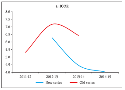
Consequent upon these changes, nominal levels of
GDP on the new base are lower relative to the old base.
Growth rates of both nominal and real GDP on the new
base are higher for each year. In terms of commonly
used indicators of productivity – the incremental
capital output ratio (ICOR) – the new series reveals a
significant improvement, but this is not corroborated
by the behaviour of other indicators, especially in an
environment characterized by declining national
savings, investment and general concerns about stalled
projects (Chart a).
 In the manufacturing sector, GVA growth is much
higher in the new series than in the earlier series. The growth of this sector appears to have been driven by
the unorganised sector, which grew by 23.3 per cent in
2012-13. Data for subsequent year, however, suggests a
slowdown of the unorganised sector, with
manufacturing growth driven mainly by the organised
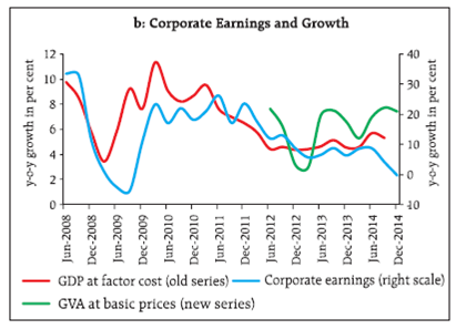
sector (Table III.B.1). While the use of MCA-21 database
could explain differences up to 2013-14, the advance
estimates for 2014-15 have used corporate sector data
– from the Reserve Bank of India (RBI) and the Bombay
Stock Exchange (BSE) – in four key components of GDP,
namely manufacturing, trade, hotels and restaurant,
and real estate. An analysis of sequential flow of
information on corporate earnings for Q3 of 2014-15
indicates that earnings growth has been much weaker
than what is implied in the new series (Chart b).
Services tax collection has also remained weak. A high
growth of 13.7 per cent (at constant prices) in “financial,
real estate and business services” reflects a possible
upward bias in estimation. It is expected that the
revised estimates for 2014-15 to be released by
end-May 2015 will incorporate better information
covering the second half of the year and provide greater
clarity on the state of economic activity at the aggregate
level.
| Table III.B.1: Manufacturing Sector Growth |
| Y-o-y growth of |
2012-13 |
2013-14 |
2014-15 |
| GVA at constant prices (base 2004-05) |
1.1 |
-0.7 |
N.A. |
| IIP |
1.3 |
-0.8 |
1.7* |
| GVA at constant prices (base 2011-12) |
6.2 |
5.3 |
6.8 |
| Organised sector |
2.5 |
6.8 |
N.A. |
| Unorganised sector |
23.3 |
0.8 |
N.A. |
| N.A. : Not available
*Pertains to April-January. |
| Table III.4: Growth in Gross Value Added at Basic Prices (Base:2011-12) |
| (Per cent) |
| |
2012-13 |
2013-14 |
2014-15 (AE) |
2013-14 |
2014-15 |
| Growth |
Share |
Q1 |
Q2 |
Q3 |
Q4 |
Q1 |
Q2 |
Q3 |
| I. Agriculture, forestry & fishing |
1.2 |
3.7 |
1.1 |
16.2 |
2.7 |
3.6 |
3.8 |
4.4 |
3.5 |
2.0 |
-0.4 |
| II. Industry |
5.1 |
5.3 |
6.5 |
23.2 |
5.9 |
4.2 |
5.5 |
5.5 |
6.5 |
5.5 |
4.6 |
| (i) Mining & quarrying |
-0.2 |
5.4 |
2.3 |
2.9 |
0.8 |
4.5 |
4.2 |
11.5 |
5.1 |
2.4 |
2.9 |
| (ii) Manufacturing |
6.2 |
5.3 |
6.8 |
18.0 |
7.2 |
3.8 |
5.9 |
4.4 |
6.3 |
5.6 |
4.2 |
| (iii) Electricity, gas, water supply & other utilities |
4.0 |
4.8 |
9.6 |
2.4 |
2.8 |
6.5 |
3.9 |
5.9 |
10.1 |
8.7 |
10.1 |
| III. Services |
6.0 |
8.1 |
9.8 |
60.6 |
8.9 |
9.7 |
8.3 |
5.6 |
8.1 |
9.8 |
11.7 |
| (i) Construction |
-4.3 |
2.5 |
4.5 |
8.0 |
1.5 |
3.5 |
3.8 |
1.2 |
5.1 |
7.2 |
1.7 |
| (ii) Trade, hotels, transport, communication and services related to broadcasting |
9.6 |
11.1 |
8.4 |
18.9 |
10.3 |
11.9 |
12.4 |
9.9 |
9.4 |
8.7 |
7.2 |
| (iii) Financial, real estate & professional services |
8.8 |
7.9 |
13.7 |
20.9 |
7.7 |
11.9 |
5.7 |
5.5 |
11.9 |
13.8 |
15.9 |
| (iv) Public administration, defence and other services |
4.7 |
7.9 |
9.0 |
12.8 |
14.4 |
6.9 |
9.1 |
2.4 |
1.9 |
6.0 |
20.0 |
| IV. GVA at basic price |
4.9 |
6.6 |
7.5 |
100.0 |
7.2 |
7.5 |
6.6 |
5.3 |
7.0 |
7.8 |
7.5 |
| Source: Central Statistics Office. AE: Advanced Estimates |
III.3 Output Gap
Uncertainty about the true value of macroeconomic
variables is a formidable challenge for policy-making,
particularly when data revisions result in information
on the same variable for the same year computed at
different times conveying different trends. The recent
revisions in national accounts pose a challenge in
terms of assessing the state of the business cycle and
the position at which the economy is poised on it. Key
to the setting of policies that modulate aggregate
demand is a good ‘fix’ on the level of output relative
to the economy’s potential. Estimating potential
output from historical data is difficult even in the best
of times. It has become much more complex in the
aftermath of the global financial crisis when potential
output across the world is likely to have fallen, led by decline in productivity. The critical issue is: do recent
revisions to India’s national accounts capture this
phenomenon? Empirical assessment suggests that
overestimation of potential output can be costly, in
terms of greater macroeconomic volatility and/or an
acceleration of inflation getting entrenched (IMF,
2011)2. A production function approach to estimating
potential output indicates a sharp decline in the
contribution of total factor productivity to potential
output. Various time series estimates of potential
output – without imposing any a priori judgment
relating to the structural interpretation of the new
GVA series – suggest that in terms of levels, the output
gap has remained negative since 2012-13, although
the gap is gradually closing (Box III.2).
The latest round of the Order Books, Inventory and
Capacity Utilisation Survey (OBICUS) of the Reserve
Bank reveals that capacity utilisation (CU) remained
range-bound in Q3 of 2014-15 as compared to the
previous quarter and declined over its level a year ago
(Chart III.7).
An overall assessment of the state of the real economy
points to recovery gaining ground slowly. Significant slack and structural rigidities continue to hold back a
sharp revival in investment demand. Lack of certainty
about cash flows from new investment projects is
contributing to the lacklustre investment cycle.
Unless structural reforms unleash productivity gains
going forward, lower saving and investment rates
could become a risk to stronger recovery. Recent
reform measures in the infrastructure sector, including
target-based progress on national highways,
encouraging FDI in railways and defence, plans to
start power plants in the private sector with all
approvals in place, bringing in the requisite
amendments in the Land Acquisition Act to expedite
project clearances and coal block auctions are expected
to address infrastructure bottlenecks and boost
medium term growth prospects.
Box III.2: Potential Output
Empirical estimates of the output gap at the aggregate
level and indicator/survey based information for major
sectors of the economy can provide an assessment of
slack in the economy. Potential output3, however, is
difficult to measure and is subject to estimation errors.
The recent revision in national accounts data which
shows major level differences in old and new series
(at constant prices) for the last four years (2011-12 to
2014-15) imparts further complexity to the estimation,
given the lack of data for previous years under the new
series.
In the absence of high-frequency and regularly updated
data on capital stock and labour in the Indian context,
estimates of potential growth through a structural
production function approach can, at best, be regarded
as indicative rather than definitive, with the results
suggesting a sharp decline in the contribution of
total factor productivity, as set out earlier. A useful
alternative to the production function approach is to
use time series methods that can estimate potential
output solely from information contained in the past data, however short their history may be. Use of various
univariate filtering techniques such as Hodrick-Prescott
(HP) and Kalman filters, and a multivariate filter
constructed from spliced quarterly GVA series, indicate
that the output gap (i.e., actual output minus potential
output) has been negative since 2012-13, irrespective of
the technique (Chart a).
IV. Financial Markets and Liquidity Conditions
Amidst abundant global liquidity and risk-on risk-off fluctuations in investor appetite, financial markets in India
rallied strongly in the second half of 2014-15, supported by improvement in domestic macroeconomic conditions.
Liquidity was comfortable in all segments and this was reflected in a pick-up in turnover, softening of interest rates,
an appreciating bias in the exchange rate of the rupee and equity markets scaling historic highs.
Since the MPR of September 2014, domestic financial
markets have been buoyed through Q3 and Q4 of
2014-15 by the global search for yields as fears of
imminent normalisation of US monetary policy receded
and ultra-accommodative monetary easing commenced
in the euro area and Japan. Barring sporadic volatility
sparked by incoming data, India became a preferred
destination in portfolio reallocations, with discernible
differentiation vis-à-vis other EMEs. Liquidity conditions
were expansionary in all segments, spurring trading
activity.
IV.1 Financial Markets
In the money markets, interest rates eased during Q3,
barring intermittent spikes around the third week of
October due to festival-related pick-up in currency
demand, and again in the second half of December on
account of advance tax payments and quarter-end
balance sheet adjustments. The shift in the monetary
policy stance steered by two cuts in the policy repo rate
enabled interest rates to ease further during Q4.
Pro-active liquidity management under the new
operating procedure of monetary policy has
played a key role in the seamless transmission of policy
impulses through the money markets. There has also
been a marked ebbing of daily volatility measured
through generalised autoregressive conditional heteroskedasticity (GARCH), although these estimates
for the end of 2014-15 tend to be strongly influenced
by the year-end spike in call rates (Chart IV.1). In this
context, the Agreement on the Monetary Policy
Framework enjoins the Reserve Bank to set out in the
public domain the operating target and procedure of
monetary policy and any changes therein that are
effected from time to time (Box IV.1).
Other money market segments moved in consonance
with the call money market. With the steady migration
of activity to collateralised segments, viz., collateralised
borrowing and lending obligation (CBLO) and market
repo, call money volumes have thinned, currently
accounting for about 10-11 per cent of the total
overnight volume (Chart IV.2). This reflects preference
for collateralised funding as well as improvements in
the microstructure such as co-terminus settlement of
market repo and outright trade in Government
securities. Trading in the call money market tends to
be skewed by its microstructure – over 70 per cent of
the activity is concentrated in the opening hour and
closing hour of trading; top five borrowers accounting
for about 50 per cent of total daily call volumes on
average (Chart IV.3). These features have occasionally
accentuated volatility in the call money market,
particularly in Q4.
Box IV.1: Operating Target and Operating Procedure of Monetary Policy
The Policy Rate
The fixed overnight repurchase (repo) rate under
the Liquidity Adjustment Facility (LAF) is the single
monetary policy rate.
The Operating Target of Monetary Policy
The weighted average call money rate (WACR) is the
operating target of monetary policy.
The Operating Procedure of Monetary Policy
Once the policy rate is announced in the Bank’s
statements on monetary policy, the operating
procedure aims at modulating liquidity conditions so
as to achieve the operating target, i.e., to anchor the
WACR around the policy rate. This is the first leg of
monetary policy transmission to the financial system
and the economy.
Liquidity Management
Pro-active liquidity management is the mechanism
through which the operating target is achieved. The
main features of the revised liquidity management
framework announced on August 22, 2014 and
implemented since September 5 are as follows: (i)
assured access to central bank liquidity of one per
cent of banks’ net demand and time liabilities (NDTL)
comprising 0.25 per cent of NDTL provided through
overnight fixed rate repo auctions conducted daily at
the policy rate, and 0.75 per cent of NDTL provided
through 14-day variable rate term repo auctions
conducted on every Tuesday and Friday; (ii) fine-tuning
operations through variable rate repo/reverse repo
auctions of maturities ranging from overnight to 28 days to even out frictional liquidity mismatches that
occur in spite of assured liquidity operations; and
(iii) outright open market operations through auctions
and anonymous screen-based trading on the Negotiated
Dealing System- Order Matching (NDS-OM) platform to
manage enduring liquidity mismatches.
Special operations are also conducted on holidays to
help market participants tide over pressures emanating
from one-off events such as tax payments, government
spending, balance sheet adjustments and payment and
settlement requirements.
Standing Facilities
A Marginal Standing Facility (MSF) allows market
participants to access central bank liquidity at the
end of the day (including Saturdays) over and above
regular and fine-tuning operations by using up to 2 per
cent of their stipulated Statutory Liquidity Ratio (SLR)
holdings of government securities in addition to excess
SLR as collateral at a rate set at 100 basis points above
the policy rate.
Fixed rate daily overnight reverse repo auctions are
conducted at the end of the day (including Saturdays)
to allow market participants to place surplus liquidity
with the Reserve Bank at a rate set at 100 basis points
below the policy rate. The fixed rate daily overnight
reverse repo operates as a de facto standing facility.
The MSF rate and the fixed overnight reverse repo
rate define an informal corridor for limiting intra-day
variations in the call rate.
The market for commercial paper (CPs) picked up
momentum during Q3 and Q4 (up to March 15), with
issuances of CPs growing y-o-y by 25 per cent and 49
per cent, respectively. This reflected some substitution
of short-term bank credit due to tight bank lending
conditions. The weighted average discount rate of CPs
softened from 8.9 per cent during the second half of
September 2014 to 8.5 per cent in the second half of
January 2015, before hardening to 8.8 per cent in the
first half of March 2015.
In the Government securities (G-sec) market, yields
softened through Q3, barring some spikes during the
second half of December 2014 due to the Ukrainian
crisis followed by the Russian currency crisis. Buoyant
investor sentiment conditioned by the ongoing
disinflation in India and expectations of monetary policy easing helped the market to shrug off the impact
of the Federal Reserve completely exiting quantitative
easing (QE) in October. The OPEC’s decision in
November 2014 not to cut production strengthened
market sentiment and reinforced the decline in G-sec
yields. During the global sell-off triggered by the
depreciation of the Ruble, however, the 10-year generic
yield jumped by 15 basis points on December 16 – the
largest increase on any single day during the second
half of 2014-15.
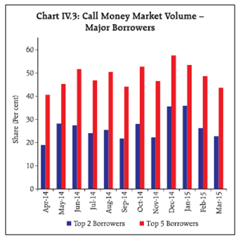 As the Russian currency crisis abated, G-sec yields
declined in Q4, aided by the softness in international
crude oil prices, fall in US treasury yields and
resumption of flows into the domestic foreign
exchange market. G-sec yields hardened transiently
in response to the reduction in the SLR in February
and the broadly unchanged size of the market
borrowing programme announced in the Union
Budget. As in the past, recourse to Treasury Bill
auctions in February and March, notwithstanding
large redemptions, inverted the G-sec yield curve,
reflecting the reluctance of market participants to part
with liquidity as the balance sheet date approached.
Barring these episodes, the G-sec market was rangebound
during Q3 and Q4 with a downward shift in
the yield curve (Chart IV.4). The 10- year yield declined
by 72 basis points from 8.52 per cent at the end of
September 2014 to 7.80 per cent on March 31, 2015.
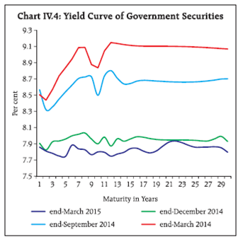 Foreign portfolio investors’ (FPIs) investment in G-secs
stood at `1,529 billion as on March 31, 2015. With the exhaustion of the limit for investment in G-secs
(US$ 30 billion), FPIs invested in debt mutual funds
allowed under the limit of US$ 51 billion for investment
in corporate debt, indirectly expanding their investment
in G-secs (Chart IV.5).
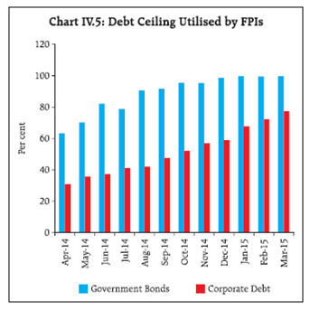 Activity in the corporate bond market also gathered
pace in Q3 and Q4, driven by private placements which
recorded a y-o-y growth of 112 per cent. On the other
hand, amounts mobilised through public issues
declined through this period (up to February). The
significant increase in resource mobilisation through
corporate bonds could be reflecting substitution effects
since bank credit growth has remained subdued in conjunction with tight credit conditions. FPIs’
investment in corporate bonds stood at `1,890 billion
as on March 31, 2015, accounting for 77 per cent of the
limit, and as a consequence, secondary market trading
volumes surged by 51 per cent (y-o-y) in the second half
of 2014-15. Yields of AAA rated corporate bonds
generally moved in tandem with G-sec yields, but
hardened somewhat in March (Chart IV.6).
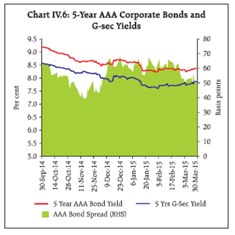 Notwithstanding increased resource mobilisation
through corporate bonds and CPs, the flow of financial
resources to the commercial sector remained lower
during 2014-15 than a year ago, mainly due to the
deceleration in non-food credit.
In the foreign exchange market, the predominant driver
has been robust capital flows that started from March
2014. The exchange rate of the rupee moved in a narrow
range of `61.04 - 62.14 per US$ but with an upward bias
through most of Q3. From December 10, however, the
rupee experienced downward pressures, slipping to a
recent low of `63.75 on December 30 on a combination
of factors – spillovers from the Russian currency crisis;
month-end purchases by oil marketing companies;
profit booking by FPIs; weak readings on industrial
output, and the relentless strengthening of the US
dollar. By the second week of January 2015, volatility
in the spot market ebbed and the rupee resumed
trading with an appreciating bias on the resumption of
FPI flows, abating of the Russian currency crisis and a
sharp fall in the trade deficit (Chart IV.7). The ECB’s
announcement of QE on January 22 and sustained softening of international crude oil prices added to the
positive sentiment in the exchange market. In the
second week of February 2015, incoming strong US
non-farm payroll data set off a slide across emerging
markets’ currency and equity markets. Range-bound
trading with modest gains followed the dovish
comments from the Federal Reserve in March regarding
the timeframe for raising its policy rate. In real effective
terms, the rupee appreciated over its level at the end
of March 2014 on account of persisting inflation
differentials vis-à-vis trading partners (Table IV.1).
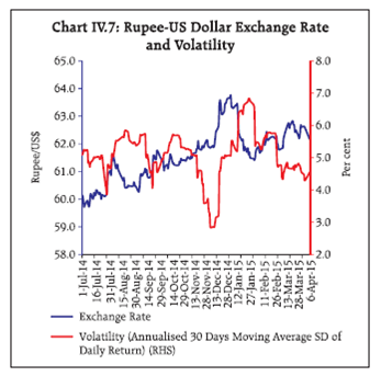 The forward market also exhibited heightened activity
in Q3, with the six-month forward premium declining
from 8.16 per cent on October 9 to 7.13 per cent on
December 26. In Q4, however, the forward premia
hardened somewhat from the second half of February
on increasing demand.
Barring soft patches, equity markets rallied through the
second half of 2014-15, scaling all-time highs. Indian indices were among the better performing in the world,
with significantly attractive valuations relative to
fundamentals and the cross-country EME experience.
Some of these gains were pared during December 2014
by pessimism triggered by fears of earlier than expected
reversal in the US interest rate cycle, uncertainty
relating to Greece and geo-political tensions in the
Ukraine and the Middle East. Equity markets, however,
started gaining again from the beginning of January
2015 on resumption of portfolio investment flows
(Chart IV.8). Buoyant sentiment bounced back with the
Reserve Bank’s announcement of a cut in the policy
repo rate on January 15, and the BSE Sensex reached a
historic high closing at 29,682 on January 29, 2015. In
the early part of February, equity markets gave up some
gains on concerns following the results of Delhi
elections, weak results reported by some big corporates,
poor Chinese trade data and decline in European stocks.
In the second half of the month, however, equity
markets recovered and gained strength with the
announcement of the Union Budget 2015-16 as also
passing of key legislations relating to coal, mining and
insurance susequently. During March 2015, the stock
market eased moderately on global cues.
| Table IV.1: Nominal and Real Effective Exchange Rates: Trade-Based (Base: 2004-05=100) |
| Item |
Index
Mar 2015
(P) |
Appreciation (+) /
Depreciation (-) (per cent) |
| Mar 2015 over Mar 2014 |
Mar 2014 over Mar 2013 |
| 36-currency REER |
113.46 |
9.3 |
-3.9 |
| 36-currency NEER |
76.85 |
6.9 |
-8.6 |
| 6-currency REER |
125.22 |
11.9 |
-6.8 |
| 6-currency NEER |
71.33 |
7.3 |
-12.6 |
| `/ US$ (As on March 31) |
62.59 |
-2.4 |
-10.8 |
| `/Euro (As on March 31) |
67.51 |
24.7 |
-16.3 |
P: Provisional.
Note: REER figures are based on Consumer Price Index (Combined).
|
In the primary market, Qualified Institutional
Placement (QIP) was moderate at `41 billion while
equity and debt issues declined to `34 billion during
Q3. On the other hand, private placements of corporate
bonds and mutual funds spurted to `1,240 billion and
`574 billion, respectively. There has already been some improvement in resource mobilisation in Q4 in
response to investment-friendly measures announced
in the Union Budget 2015-16 and steps taken by the
SEBI to streamline existing regulations relating to public
shareholding of state-owned companies.
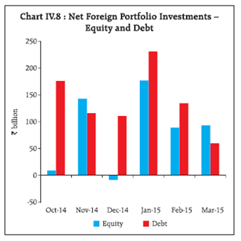 In the credit market, subdued activity in the first half
of the year picked up from Q3 as banks shifted their
portfolios towards retail lending, especially housing.
Credit flow to the industrial sector – particularly to food
processing and basic metals – and services, also
improved modestly (Chart IV.9). Reflecting the generally
sluggish demand for credit as also regulatory
requirements relating to the liquidity coverage ratio
(LCR), banks’ investments in G-secs, on the other hand,
showed a sharp increase during 2014-15. Excess SLR
holdings of banks increased significantly as a
consequence. Banks have been rebalancing their
lending portfolio away from sectors in which their
assets are under stress to relatively stress free sectors
such as retail housing and automobiles.
Following the 50 basis points reduction in the policy
rate in Q4, 22 banks have reduced their median term
deposit rates in the range of 7-53 bps while 14 banks
reduced their base rates in the range of 10-50 bps.
IV.2. Liquidity Conditions
Broad money (M3) growth remained low during Q3 and
Q4. With credit and deposit growth moving broadly in
tandem, liquidity conditions in the system remained
comfortable throughout, barring transient liquidity mismatches due to frictional factors alluded to earlier
(Chart IV.10). Currency demand started picking up since
Q3 with the festival season and drained some liquidity,
but timely liquidity provision by the Reserve Bank
smoothened these short-lived spikes. The provision of
primary liquidity was augmented by the large expansion
in net foreign assets of the Reserve Bank. Active
sterilisation operations, however, contained the growth
of reserve money (Chart IV.11).
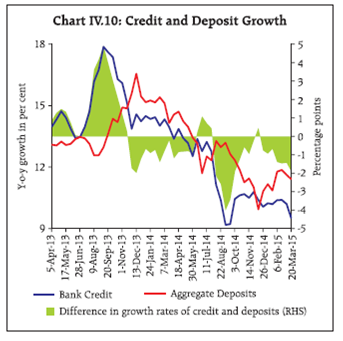 Liquidity conditions improved during Q3 of 2014-15,
reflecting a confluence of structural and frictional
factors, barring temporary pressures around festival days, mid-December advance tax payments and quarterend
window dressing. In Q4, liquidity conditions
tightened since the second week of January 2015 with
cutbacks in government spending, pick-up in credit
demand and seasonal increase in currency demand.
The Reserve Bank’s pro-active liquidity management
operations ensured that the call rates stayed range
bound around the policy rate, reducing day-to-day
volatility (Chart IV.12).
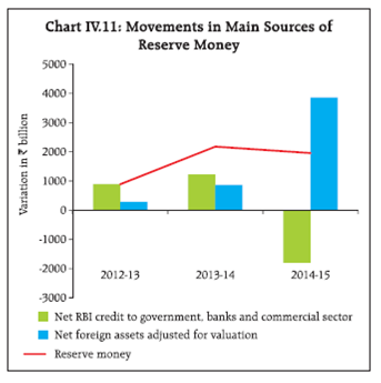
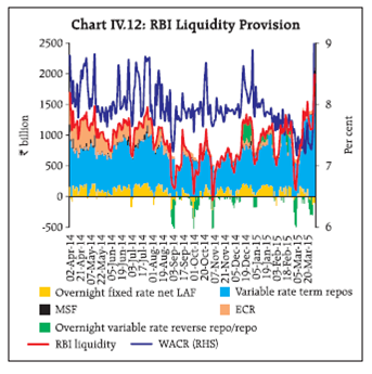 In pursuance of the Dr. Urjit R. Patel Committee’s
recommendation to move away from sector-specific
refinance, the export credit refinance (ECR) limit was
reduced in three phases starting June 2014 and finally
subsumed in the provision of system level liquidity
with effect from February 7, 2015. As a further measure
to facilitate smoother operations, the Reserve Bank
started conducting reverse repo and MSF operations
on all Saturdays, effective February 21, 2015.
Overall, financial markets traded on a bullish note
during the second half of 2014-15 against the backdrop
of improved domestic fundamentals and a global
appetite for risk. The evolution of overall global
liquidity conditions has been conditioned by
expectations relating to high intensity events such as
the lift-off of US interest rates, monetary accommodation
elsewhere and geo-political flashpoints. Liquidity
conditions remained stable and movements in the
overnight call money rate were, by and large, anchored
around the policy repo rate.
V. External Environment
Global economic recovery remained tepid and divergent across economies, with most EMEs experiencing slowdown.
While AEs remain susceptible to the risk of deflation, inflationary pressures subsided in key EMEs giving leeway
for easing monetary policy. Global commodity prices continue to decline. Financial markets were buoyant but volatile
in pricing in policy developments in major economies.
In the months following the MPR of September 2014,
global economic activity appears to be stabilising, but
with markedly divergent growth profiles between
advanced and emerging economies, and between
commodity exporters and importers. The collapse of
international commodity prices, especially of crude oil,
seems to have reallocated demand across economies.
Monetary policy stances across countries have been
easing, including unconventionally, and market
expectations on the timing of the US monetary policy
normalisation have been pushed back. In response,
there have been large movements in exchange rates
and other asset prices. Reflecting risk appetite and
search for yield, long-term yields have fallen to record
lows amidst heightened volatility in financial markets.
For commodity exporters, however, risk spreads
have widened and currency depreciations have been
sizable. Thus, even though financial conditions are
easy and are being reflected in financial asset prices,
the outlook for global growth remains moderate, held
back by still-weak demand.
V.1. Global Economic Conditions
In the United States, growth has been firming up,
aided by improving labour and housing market
conditions. The sharp appreciation in the US dollar in
recent months could, however, dampen prospects for
exports. In the Euro area, economic conditions remain
weak although some pick-up in Q4 of 2014 and the
early months of 2015 is being observed, supported by
lower crude prices and the depreciation in the euro
as well as increased bank lending. The contraction
of activity in Japan moderated in the final quarter
of 2014, with mixed signals from higher frequency
data in the beginning of 2015 - consumer confidence
and exports show improvement, but retail sales and
industrial production have contracted.
Most EMEs continue to decelerate due to subdued
external demand, political uncertainties and domestic supply-side constraints. In China, activity has slowed
over the second half of 2014 and Q1 of 2015 as
investment demand lost pace and the real estate sector
weakened on deleveraging and financial repair among
households and corporations. The Russian economy
slowed sharply due to falling oil prices and Western
sanctions. Contraction continues in Brazil as high
inflation squeezes domestic demand. Falling oil and
commodity prices also weighed on growth prospects
of countries in the Middle East, Eastern Europe and
Latin America (Table V.1).
| Table V.1: Real GDP Growth (Y-o-Y, Per cent) |
| Period |
Q1-2014 |
Q2-2014 |
Q3-2014 |
Q4-2014 |
2015P |
| Advanced Economies |
| United States |
1.9 |
2.6 |
2.7 |
2.4 |
3.6 |
| Euro area |
1.1 |
0.8 |
0.8 |
0.9 |
1.2 |
| Japan |
2.1 |
-0.4 |
-1.4 |
-0.7 |
0.6 |
| United Kingdom |
2.7 |
2.9 |
2.8 |
3.0 |
2.7 |
| Canada |
2.1 |
2.6 |
2.7 |
2.6 |
2.3 |
| Emerging Market Economies |
| China |
7.4 |
7.5 |
7.3 |
7.3 |
6.8 |
| Russia* |
0.6 |
0.7 |
0.9 |
0.4 |
-3.0 |
| Brazil* |
2.7 |
-1.2 |
-0.6 |
-0.2 |
0.3 |
| Mexico |
0.9 |
2.8 |
2.2 |
2.6 |
3.2 |
| South Africa |
2.1 |
1.3 |
1.5 |
1.3 |
2.1 |
| Memo Items: |
2014 |
2015P |
| World Output |
3.3 |
3.5 |
| World Trade Volume |
3.1 |
3.8 |
P: Projection,
*not seasonally adjusted
Sources: OECD, IMF and Bloomberg. |
Overall, although the near-term outlook is improving
slowly, AEs are yet to fully recover from the aftereffects
of the global financial crisis. EMEs face the
challenge of addressing persistent negative output
gaps and falling growth potential, which yields a
more subdued near-term outlook for them. In fact,
the sluggish global recovery over the course of 2014
and 2015 so far has warranted successive downward
adjustments to forecasts the world over, raising
concerns of ‘secular stagnation’ (Box V.I).
Box V.1: Secular Stagnation: A Post-crisis Concern
Despite ultra accommodative monetary policies pursued
for a considerable period, AEs continue to languish,
raising fears that they may be suffering from secular
stagnation. The theory of secular stagnation (Hansen,
1939) is Keynesian in emphasising the role of deficient
demand evident in a saving glut. Supply-side factors
are also at play in stagnating long-run growth - slow
population growth and shrinking working-age labour
supply; slow technological progress; and low returns on
human capital (Gordon, 2014). The combination of these
forces is driving down AEs to an equilibrium trap of
lower investment and lower potential growth. Thus, the
slowdown in AEs is more of a structural phenomenon,
rather than a cyclical outcome of the financial crisis.
On the other hand, deleveraging in the financial sector,
balance sheet repair and resolution is taking its toll on
growth in AEs (Chart V.B.1).
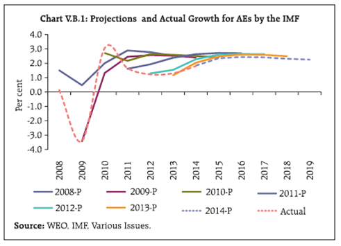 It has been argued that potential output in the US
economy is now 10 per cent below its level in 2007
(Chart V.B.2), i.e., no progress has been made in restoring
GDP to its potential (Summers, 2014a). The aggregate
employment/population ratio tends to corroborate
this view, even when the working age population is considered.
Has the future potential of the economy become
impaired? Slower total factor productivity accounts for
the smallest part of the downward trend in potential,
whereas the largest part is associated with reduced
capital investment, followed closely by reduced labour
input. Similar evidence is discernible in the case of
Japan and Europe.
Changes in the structure of the economy have also led to
a significant shift in the natural balance between saving
and investment, causing a decline in the equilibrium or
normal real rate of interest that is associated with full
employment (King and Low, 2014). This could portend
increased vulnerability to financial stability in the future
on a global basis.
These developments suggest that as a long-term strategy,
employing monetary policy to raise potential output
appears to have reached its limits. Raising the level of
demand through regulatory and tax reforms that would
promote private investment, policies that promote
exports and public investments could be a more effective
strategy. Model simulations for the US suggest that a
one per cent increase in the budget deficit directed at
government spending maintained for five years produces
a substantial demand response even after allowing for
labour withdrawal effects (Chart V.B.3) - the potential
multiplier can be quite large - with a reduction in the
long-run debt to GDP ratio (Summers, 2014b).
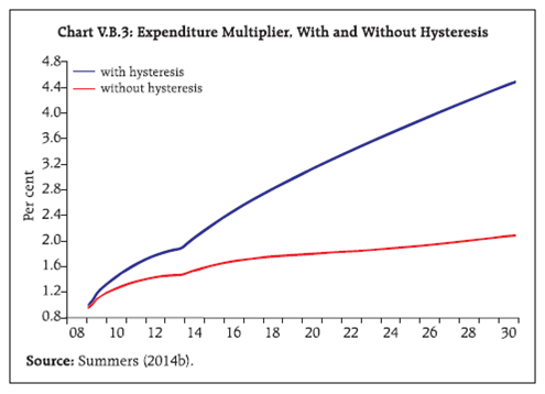 The jury is still out on whether or not AEs face secular
stagnation. An alternative view is that it is just a
prolonged business cycle, reflection of temporary
headwinds and misguided fiscal contraction (Beckworth,
2014). Understandably, there is no consensus on the
appropriate policy responses: fiscal policy to stimulate
aggregate demand through infrastructure investment;
persistently low interest rates to encourage demand; structural reforms to address supply side constraints;
technological innovations (Brynjolfsson and McAfee,
2014) or a judicious combination.
References:
Beckworth, D. (2014), “Here’s why Larry Summers is
wrong about secular stagnation”, Wall Street Journal.
Brynjolfsson, Erik and Andrew McAfee (2014), The
Second Machine Age: Work, Progress, and Prosperity in a
Time of Brilliant Technologies, W. W. Norton & Company.
Gordon, R (2014), “The Demise of U.S. Economic Growth:
Restatement, Rebuttal, and Reflections”, NBER Working
Paper No. 19895.
Hansen, A.H. (1939), “Economic Progress and Declining
Population Growth”, American Economic Review, Vol. 29
(1), pp. 1-15.
King, Mervyn and David Low (2014), “Measuring the
‘’World’’ Real Interest Rate”, NBER Working Paper No.
19887.
Summers, L.H. (2014a), Reflections on the ‘New
Secular Stagnation Hypothesis’ in C. Teulings and
R.Baldwin (Eds.) Secular Stagnation: Facts, Causes and
Cures (pp.27-38), A Vox EU.org.Book, CEPR Press.
Summers, L.H. (2014b), “US Economic Prospects: Secular
Stagnation, Hysteresis, and the Zero Lower Bound”,
Business Economics, Vol. 49 (2), pp. 65-74.
The pace of global trade continues to be weighed
down by both cyclical and structural factors, with
world trade volume growing by only 3.1 per cent in
2014 - well below the pre-crisis trend (IMF, 2015).1
The impact of the growth slowdown in China,
Russia, the Euro area and Japan on world trade has
been significant, aggravated by weaker activity in
some major oil exporters. Even though world trade
growth is expected to pick up moderately along
with improvement in global output in 2015 (IMF,
2015), risks continue to tilt downwards, given the
subdued conditions characterising global demand and
international commodity prices. Incoming data on
most EMEs show contraction in exports in the first
two months of 2015.
V.2. Global Inflation Developments
Inflation continues to drift downward in AEs and
many EMEs albeit in varying degrees. Given weak demand conditions, falling commodity prices has
made deflation a major concern for many AEs. The
Euro area is struggling to emerge out of a deflationary
spiral with CPI inflation of (-)0.1 per cent in March.
In the US and the UK, inflation has been declining
since the second half of 2014, with zero inflation in
February in both countries. For the UK, low food and
fuel prices have been the prime factors for keeping
inflation low. In the US, appreciation of the dollar
has also had a disinflationary effect. In Japan too, CPI
inflation has shrugged off the effects of the hike in
the consumption tax in April 2014 and has steadily
fallen to 2.2 per cent, primarily driven down by falling
commodity prices (Chart V.1a).
Although EMEs, in general, have benefited from the
sharp fall in commodity prices, inflation has remained
stubbornly high in a few countries. While China faces
the risk of deflation due to weak domestic demand and falling factory prices, the slump in oil prices has given
some respite to inflation in Indonesia, South Africa
and Turkey. By contrast, inflationary pressures remain
high in Brazil and Russia, attributable to domestic
factors and substantial currency depreciation (Chart
V.1b).
 Since August 2014, strong supply positions have led
to a drastic fall in world energy prices, with Brent and
WTI crude oil prices falling below US$ 50 per barrel
in January 2015 (Chart V.2). Since then there have
been intermittent bouts of volatility, driven by factors
such as decline in US rig counts, relatively positive
data on the US economy and disturbances in the
Middle East. Most non-energy prices have also been
on a steady decline. Global food prices continue to
slide downward, underpinned by strong production
expectations, robust inventories, the strong US dollar
and limited demand from major importers like China.
Looking ahead, commodity prices will likely remain
stable as slack in the global economy persists.
Tepid and uneven economic recovery across major
economies could intensify disinflationary pressures.
On the other hand, monetary policy easing measures
undertaken by major central banks should support
demand.
V.3. Monetary Policy Stance
Faced by the combination of deflationary/
disinflationary pressures and weak growth,
central banks in both AEs and EMEs have pursued
accommodative monetary policies. In the US, monetary
policy remains highly accommodative with interest rates close to zero even after the cessation of the Fed’s
asset purchases in October. Notwithstanding forward
guidance in March setting the stage for lifting its policy
rate, markets anticipate a relaxed approach from the
Fed in this regard. Facing persistent deflation, the Bank
of Japan has continued with its target of monetary
base expansion of 80 trillion yen per year. The ECB
began its asset purchase programme since March 2015
which, in turn, has produced sizable depreciation of
the euro and taken long-term bond yields to new lows.
Some countries have resorted to negative interest rate
policy to counter high real interest rates arising due to
deflationary pressures (Chart V.3a).
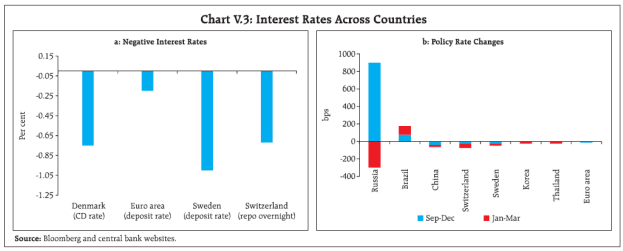 Many EMEs have eased their policy stances as
inflationary pressures subsided on weak domestic demand and the sharp fall in energy prices. China
followed up deposit/lending rate cuts in November
2014 and February with reduction in reserve
requirements in February and other measures to
reduce financing costs. Other EMEs such as Thailand
and Korea have also reduced policy rates in quick
succession to protect their external competitiveness.
Turkey and Indonesia eased their policy rates as the
inflation outlook improved. Stricken severely by the
fall in global oil prices and Western sanctions, Russia
cut its policy rate twice in Q1 of 2015 (January and
March). Brazil has been an exception, relentlessly
raising policy rates up to a six-year high in March; a
weakening currency has further exacerbated already
high inflationary pressures (Chart V.3b).
Yet most policy shifts by central banks have been
apparently driven by the weak economy and exchange
rate concerns rather than financial stability, implying
competitive devaluations.
VI.4. International Financial Markets
Financial markets have been volatile since mid-2014,
triggered by data releases in the US and the Fed’s
statements on the normalisation of monetary policy.
Political tensions in Europe relating to Greece, lower oil
prices and country-specific events have also impacted
investor sentiment. Unprecedented low interest rates
and compressed risk premia have led to a precipitous
fall in long-term government bond yields while raising
most asset prices to near record highs as the search for
yield pushed investors to riskier assets (Chart V.4a).
Further easing of monetary policy propped up global
equity markets in Q1 of 2015, particularly in AEs,
albeit preceded by bouts of volatility in the second
half of 2014 (Chart V.4b).
Capital flows to EMEs subsided in the second half
of 2014, as growth remained lacklustre. Falling
commodity prices and the shifting trajectory of US
monetary policy heightened risk aversion. However,
portfolio flows to a few EMEs rebounded in Q1 of
2015 following the announcement of the ECB’s QE
programme. With markets reading Fed’s forward
guidance in its March statement as dovish, volatility
returned in portfolio flows to EMEs and investors
tended to discriminate against countries with relatively
weaker domestic macroeconomic fundamentals.
The US dollar has gained against major currencies and
most EME currencies. Since end-June 2014, the dollar
index has gained about 20 per cent both in nominal
and real terms against major currencies.
In sum, the uncertainty surrounding near-term
prospects and the underlying drivers of future crude
oil prices have added a new dimension to the global
growth outlook. While on the upside, lower oil prices
could spur global demand by increasing the purchasing
power of oil importers, on the flipside, oil exporters
could be adversely affected. With divergent monetary
policy stances across major economies, risks related
to shifts in market sentiment and resultant bouts of
volatility in capital flows and currency markets remain
elevated.
ABBREVIATIONS
| AAY |
Antyodaya Anna Yojana |
| AE |
Advance Estimates |
| AEs |
Advanced Economies |
| AL |
Agricultural Labourers |
| APL |
Above Poverty Line |
| APMC |
Agriculture Produce Market Committee |
| ARIMA |
Auroregressive Integrated Moving Average |
| Avg. |
Average |
| BE |
Budget Estimates |
| BEI |
Business Expectations Index |
| bn |
Billion |
| BPL |
Below Poverty Line |
| bps |
Basis Points |
| BRICS |
Brazil, Russia, India, China and South Africa |
| BSE |
Bombay Stock Exchange |
| BVAR |
Bayesian Vector Autoregression |
| CAD |
Current Account Deficit |
| CBLO |
Collateralised Borrowing and Lending Obligation |
| CEPR |
Centre for Economic Policy Research |
| CCS |
Consumer Confidence Survey |
| CD |
Certificates of Deposit |
| CES |
Consumer Expenditure Survey |
| CI |
Confidence Interval |
| CII |
Confederation of Indian Industry |
| CMIE |
Centre for Monitoring Indian Economy |
| CP |
Commercial Paper |
| CPI |
Consumer Price Index |
| CPI-AL |
Consumer Price Index - Agricultural Labourers |
| CPI-C |
Consumer Price Index- Combined |
| CPI-IW |
Consumer Price Index - Industrial Workers |
| CPI-RL |
Consumer Price Index - Rural Labourers |
| CRR |
Cash Reserve Ratio |
| CSO |
Central Statistics Office |
| CU |
Capacity Utilisation |
| ECB |
European Central Bank |
| ECR |
Export Credit Refinance |
| EMEs |
Emerging Market Economies |
| FDI |
Foreign Direct Investment |
| FED |
Federal Reserve System, USA |
| FG |
Finished Goods |
| FICCI |
Federation of Indian Chambers of Commerce and Industry |
| FIIs |
Foreign Institutional Investors |
| FIT |
Flexible Inflation Targeting |
| FPIs |
Foreign Portfolio Investors |
| FY |
Financial Year |
| GARCH |
Generalised Autoregressive Conditional Heteroskedasticity |
| GCF |
Gross Capital Formation |
| GDP |
Gross Domestic Product |
| GFD |
Gross Fiscal Deficit |
| GNDI |
Gross National Disposable Income |
| GoI |
Government of India |
| G-secs |
Government Securities |
| GVA |
Gross Value Added |
| HP |
Hodrick-Prescott |
| ICOR |
Incremental Capital Output Ratio |
| IIP |
Index of Industrial Production |
| IMF |
International Monetary Fund |
| IW |
Industrial Workers |
| LAF |
Liquidity Adjustment Facility |
| LCR |
Liquidity Coverage Ratio |
| LPG |
Liquefied Petroleum Gas |
| Ltd. |
Limited |
| M3 |
Money Supply |
| MCA |
Ministry of Corporate Affairs |
| MGNREGA |
Mahatma Gandhi National Rural Employment Guarantee Act |
| MMRP |
Modified Mixed Reference Period |
| m-o-m |
Month-on-Month |
| MOSPI |
Ministry of Statistics and Programme Implementation |
| MPR |
Monetary Policy Report |
| MSF |
Marginal Standing Facility |
| MSP |
Minimum Support Price |
| NA |
Not Available |
| NCAER |
National Council of Applied Economic Research |
| NDS-OM |
Negotiated Dealing System-Order Matching |
| NDTL |
Net Demand and Time Liabilities |
| NEER |
Nominal Effective Exchange Rate |
| NIIP |
Net International Investment Position |
| NSC |
National Statistical Commission |
| NSS |
National Sample Surveys |
| NSSO |
National Sample Survey Office |
| OBICUS |
Order Books, Inventory and Capacity Utilisation Survey |
| OECD |
Organisation of Economic Co-operation and Development |
| OMCs |
Oil Marketing Companies |
| OPEC |
Organisation of the Petroleum Exporting Countries |
| PDS |
Public Distribution System |
| POL |
Petroleum, Oil and Lubricant |
| QE |
Quantitative Easing |
| QIP |
Qualified Institutional Placement |
| q-o-q |
Quarter-on-Quarter |
| RBI |
Reserve Bank of India |
| RE |
Revised Estimates |
| REER |
Real Effective Exchange Rate |
| RL |
Rural Labourers |
| RM |
Raw Material |
| SEBI |
Securities Exchange Board of India |
| SLR |
Statutory Liquidity Ratio |
| SNA |
System of National Accounts |
| T-Bill |
Treasury Bill |
| UK |
United Kingdom |
| URP |
Uniform Reference Period |
| US |
United States |
| VAR |
Vector Autoregression |
| Vol. |
Volume |
| WACR |
Weighted Average Call Money Rate |
| WEO |
World Economic Outlook |
| WPI |
Wholesale Price Index |
| WTI |
West Texas Intermediate |
| y-o-y |
Year-on-Year |
| YTM |
Yield to Maturity |
| ZLB |
Zero Lower Bound |
|