Press Release

RBI Working Paper Series No. 07
What Explains Call Money Rate Spread in India?

^@Sunil Kumar
Anand Prakash
Krishna M Kushawaha

Abstract

¹The study focuses on various drivers of overnight inter-bank rate spread under the new liquidity management framework during July 2013 to December 2016. Applying OLS with Newey-West estimator and various GARCH models to daily data, the study finds that liquidity conditions, viz., deficit, distribution and uncertainty impact the call money rate spread adversely. A moderation in the impact of liquidity uncertainty has, however, been noticed after the introduction of fine-tuning liquidity management operations in September 2014. Other factors, viz., the quarter-end phenomenon and structural changes in the liquidity management framework have also been found impacting the call money rate spread.

Keywords: Monetary Policy, Call Money Spread, Policy Rate, Liquidity, Market Structure

JEL Classification: E43, E52, E58

Introduction

A well-developed money market is the key to effective transmission of monetary policy to financial markets and finally to the real economy. With the onset of economic reforms and the transition to indirect market-based instruments of monetary policy in the 1990s, the Reserve Bank of India (RBI) made conscious efforts to develop an efficient, stable and liquid money market by creating a favourable policy environment through appropriate institutional changes, instruments, technologies and market practices. The call money market was developed into primarily an inter-bank market, while encouraging other market participants to migrate towards collateralised segments (CBLO and market repo) of the market, thereby increasing overall market integrity.

In line with developments in the money market, India’s monetary policy framework has also undergone several transformations over the years and important landmarks are: (i) a shift from direct instruments to indirect instruments during 1990s; (ii) multiple indicators approach replacing the single indicator in 1998 with enhanced reliance on rate channels than the quantity channel for monetary policy formulation; (iii) establishing repo rate as the policy rate with a corridor and weighted average call rate (WACR) as the operating target of the monetary policy based on the recommendation of the Working Group on Operating Procedure of Monetary Policy (Chairman: Shri Deepak Mohanty); and (iv) phased revision in the operating framework of monetary policy including adoption of a new liquidity framework and consumer price index (CPI) inflation as a nominal anchor and shift to a monetary policy committee on the recommendations of the Expert Committee to Revise and Strengthen the Monetary Policy Framework (Chairman: Dr. Urjit Patel).

The monetary policy framework agreement (MPFA) signed between the RBI and Government of India on February 20, 2015 paved the way for flexible inflation targeting (FIT), setting a medium term CPI inflation target of 4 +/-2 per cent with the mid-point to be achieved by the end of 2017-18. Subsequently, with the amendment to the RBI Act on May 14, 2016, several provisions of MPFA were subsumed in the amended Act^[1] (RBI, 2016). Notwithstanding the above-mentioned changes, the call rate (inter-bank overnight rate) continues to remain at the centre of the monetary policy framework.

As the overnight inter-bank rate is the starting point of monetary policy transmission, study of its behavior becomes important from RBI’s perspective. Wurtz (2003) argues that it is pertinent for the Central Bank to understand the response of overnight inter-bank rate to the monetary policy decisions and operations as well as to other exogenous variables under the relevant operational framework^[2]. A change in overnight rate is expected to get transmitted to the entire spectrum of term structure of interest rates (as per the expectations hypothesis, the Nth-period yield is the weighted average of future overnight rates, duly adjusted for a risk/ term premium^[3]), eventually affecting the investment and savings decisions of economic agents.

Moschitz (2004) underlines the importance of understanding the behaviour of the overnight rate (i.e. short end of the yield curve) in order to explain the other interest rates across the term structure. Although level of the overnight rate is set by the extant macroeconomic conditions, its equilibrium outcome is largely conditioned by demand for and supply of bank reserves. Banks having liquidity in excess of the required reserves are in a position to lend these excess reserves in the inter-bank market. On the other hand, banks which are short of liquidity can borrow from the inter-bank market. Furthermore, banks’ decision to hold the reserves is dictated by their profit maximization behavior within the constraint of reserve requirement stipulation. Thus, various banks’ desire to hold higher or lesser reserves determines the demand for and supply of liquidity in the inter-bank market. Any mismatch between demand and supply can only be bridged by the central bank, which is the sole supplier of net liquidity to the system. Therefore, interaction of the central bank, as net supplier of reserve, with banks plays a critical role in determining the overnight interest rate. The central bank supplies liquidity to meet the demand in order to keep overnight interest rate at around the target rate, i.e., policy rate. Nonetheless, the supply shocks generated by autonomous factors, such as, government cash balances may at times outweigh net liquidity supplied by the central bank^[4].

Further, RBI has brought about several changes in the liquidity framework since July 2013 whereby liquidity available through fixed rate overnight repo under liquidity adjustment facility (LAF) has been restricted along with introduction of variable rate repos and reverse repos of various tenors and these changes have not only provided a large part of the liquidity for more than overnight tenor but also infused both competition and uncertainty with regard to availability of liquidity/ reserves. In sum, the overnight inter-bank rate is determined by various factors, which impact demand for and supply of liquidity in the banking system, including central bank’s net supply of liquidity. The most important drivers of overnight spread identified in literature are liquidity conditions, policy rate expectations, and end-of-period effects.

Though the behaviour of overnight inter-bank rate/ its spread over policy rate has been extensively researched in the case of advanced countries (especially in the euro area and USA), the paucity of such studies has been quite stark in the case of emerging market and developing economies (EMDEs). There have been very few studies on the behaviour of the overnight inter-bank rate in India. Ghosh and Bhattacharya (2009) studied the relationship between bid-ask spread and conditional volatility in the overnight money market during 1999-2006. Patra et al. (2016) evaluated the liquidity management framework by investigating performance of the first leg of transmission - from the policy rate to the operating target (overnight inter-bank rate) and gains in terms of minimizing the volatility of the operating target- thereby strengthening the conditions for efficiency in the second leg of transmission. Our study endeavors to analyse the drivers of the overnight inter-bank rate spread, i.e. difference between weighted average call rate (WACR) and policy rate (rate), under the new liquidity management framework (NLMF). During the period from July 2013 to December 2016, far-reaching changes were introduced in the liquidity management framework. We refer the liquidity management framework, which encompasses all these changes starting from July 17, 2013 as NLMF in our study. The basic idea of the study is to identify the drivers of the WACR spread after the introduction of these far reaching changes in the liquidity management framework from July 2013 (which, inter alia, include restricting banking sector’s access to fixed rate repo and proactive use of variable rate repo and reverse repo operations of various tenors by the RBI), and how they have helped in achieving close alignment of the WACR with the policy rate.

The paper contributes to the strand of literature on determinants of overnight spread, which is critical for monetary policy transmission. At the same time, this paper will help in improving the understanding about liquidity dynamics and their impact on overnight spread. We have used ordinary least square (OLS), augmented with both Newey-West estimator and ARCH effect to overcome heteroskedasticity in errors, for estimating coefficients of determination. Our main findings are that liquidity conditions, liquidity distribution and liquid uncertainty tend to raise call money spread adversely. The impact of liquidity uncertainty on WACR spread has, however, moderated after introduction of fine tuning liquidity management operations from Sept 5, 2014. Other qualitative factors that have been found driving the WACR spread are the quarter-end phenomenon, structural changes in the liquidity management framework effected in the wake of taper tantrum episode of 2013, and fine tuning liquidity management operations. As expected, the impact of fine tuning operations has been found negative, i.e., fine tuning operations reduce the spread during deficit situation and vice versa. The rest of the paper is organised as follows: Section II contains literature review; Section III explains market structure and stylized facts; possible determinants against the theoretical backdrop are discussed in Section IV; Section V contains data and methodology used for estimation; empirical results are explained in Section VI and concluding observations are given in Section VII.

II. Literature Review

Several studies, viz., Moschitz (2004); Valimaki (2006); Linzert and Schmidt (2008); Soares and Rodrigues (2011); and Beirne (2012) have explored the determinants of spread between European Overnight Rate (EONIA) and ECB’s policy rate (EONIA spread). Moschitz (2004) modeled the inter-temporal decision problems in the reserve market for both central and commercial banks and found a substantial liquidity effect with a permanent change in reserve supply leading to change in the overnight rate in the opposite direction during the reserve maintenance period. He further finds that the magnitude of liquidity effect was determined by distribution of liquidity shocks and banks’ immediate response to the supply changes was sluggish. Valimaki (2006) argues that in the wake of central bank applying a quantity oriented liquidity policy, the money market inefficiencies and banks’ risk aversion, even if the central bank’s preferences are symmetric and the markets do not anticipate any changes in the policy rates, might result in a positive spread. He further argues that in such a case, the liquidity uncertainty, which is significantly conditioned by liquidity supplied by the central bank, would be the driving force behind emergence of a positive spread.

Linzert and Schmidt (2008), while analyzing the possible determinants of EONIA spread, conclude that liquidity conditions and banks’ liquidity uncertainty put upward pressure on the EONIA spread. They also find that ECB’s liquidity policy reduces the EONIA spread when large liquidity is injected through last main refinancing operation (MRO) of the maintenance period. Overall, they conclude that structural factors, such as, central bank’s balance sheet and operational framework could play an important role in determining the EONIA spread. Soares and Rodrigues (2011) model the volatility of the EONIA spread and their results suggest that ECB found it difficult to steer the EONIA spread during the turbulent period (2008-2009) but provision of long-term liquidity was found to be effective in reducing volatility. They also detect a structural change in the behavior of the EONIA spread in reaction to shocks.

Beirne (2012) explores the factors affecting the EONIA spread before and during the crisis period 2007-2009 and finds that the impact of the liquidity on the EONIA spread was state-independent but credit and liquidity risk factors made explaining the EONIA spread complex. Interestingly, he finds that liquidity and credit risk impacted EONIA spread negatively during crisis period, which largely got reflected in shifting of money market activities to the overnight segment in the backdrop of heightened uncertainty. Beirne (2012) also concludes that the central bank is competent in dealing with liquidity risk but may not be so competent to address credit risk and, hence, there may be some merit in the central bank targeting a secured overnight rate instead of unsecured overnight rate. Hassler and Nautz (2008) argue that overnight rates play a crucial role in implementing monetary policy. Applying fractional integration techniques to examine whether the persistence of the spread between the EONIA and key policy rate has changed since the introduction of ECB’s new operational framework in March 2004, they find increased persistence of the EONIA spread, suggesting that the degree of controllability of the EONIA spread might have declined.

Whitesell (2006) evaluates reserves regimes versus interest rate corridors, which have become competing frameworks for monetary policy implementation. Rate corridors, relying on lending and deposit facilities to create ceilings and floors for overnight interest rates, evince mixed results on controlling volatility. Reserve requirements allow period-average smoothing of interest rates but, even if remunerated, are subject to reserve avoidance activities. The paper, based on various models and experiences to date, finds a continuing advantage for period average reserves, even in the presence of a rate corridor. According to the paper, the best practice policy implementation framework may include elements of both interest rate corridors and period-average reserves. Wurtz (2003) presents a complete empirical model on the spread between the EONIA rate and the key policy rate of the ECB and shows that the most important variables driving the level and the volatility of this spread are expectations about changes in the key policy rate and the projected liquidity conditions at the end of the reserve maintenance period.

Bech and Monnet (2013) have documented four stylised facts with respect to the impact of unconventional monetary policies on the price and quantity dynamics of the overnight money market. They look at six markets in developed economies and show that the surge in excess reserves drive overnight rates to a rate at which central bank remunerates reserves. Further, they illustrate how the expansion of excess reserves decreases market volume and reduces the volatility of the overnight rate. Additionally, they provide prima facie evidence that counterparty risk affects the pricing of unsecured overnight loans between banks even when the market is flush with liquidity. Neyer and Wiemers (2004), based on an interbank market model with a heterogeneous banking sector, show that positive spread between the inter-bank market rate and the central bank rate, resulting from heterogeneity among banks on account of different marginal costs of obtaining funds from the ECB, is determined by transaction costs in the inter-bank market, total liquidity needs of the banking sector, costs of obtaining funds from the central bank, and the distribution of the latter across banks. Recently, Kucuk, et al. (2014) have studied the determinants of the overnight spread in an emerging market like Turkey and have found that net liquidity deficit, liquidity uncertainty, and liquidity distribution are the most prominent drivers of overnight spread in the new monetary policy episode.

In the Indian context, few studies have attempted to examine certain aspects of the overnight inter-bank rate/ spread. Patra et al. (2016) examined the performance of liquidity management in terms of a shift from corridor play to tactical marksmanship, i.e., the liquidity operations under the new liquidity management framework have focused on keeping the WACR closely aligned with the policy rate thereby reducing the de facto width of the corridor for operational purposes. They find a high degree of precision in the RBI’s liquidity management framework and deviations of the operating target from the policy rate have become more transient in the most recent regime than before. The current regime is engendering better liquidity management with intra-period reserve maintenance flux getting evened out and final day effects during the maintenance period becoming statistically insignificant. They also conclude that volatility in the call rate has distinctly declined in the current period relative to earlier ones, improving monetary policy transmission across the money markets. Ghosh and Bhattacharya (2009), using a GARCH model to estimate conditional volatility in the Indian overnight money market during the period 1999–2006, find that the bid-ask spread in the overnight market was positively related to conditional volatility during 1999–2002. They detect a structural break from 2002 in this relationship and find that lagged spread, along with conditional variance of the call rate, played an important role in determining spread during 2002–2006, indicating an improvement in market microstructure.

III. Market Structure and Stylized Facts

Overnight money market in India comprises of three segments viz., inter-bank call money, collateralised borrowing and lending obligation (CBLO), and market repo. The first segment is unsecured while the latter two segments are secured. The CBLO was introduced in 2003 to provide an alternative avenue for short-term funds for market participants, especially mutual funds and non-banking finance companies (NBFCs), and to pave the way for gradual exit of non-banks from the call money market. As envisaged, the market participants shifted to CBLO for short-term funds in a big way and the call money turned into a pure inter-bank market (including Primary Dealers) in 2005. The overnight market has made rapid strides in the last decade with phenomenal growth in trading volumes, albeit, the share of call money has declined significantly with market participants, including banks, increasingly relying on collateralised overnight segments, especially CBLO, for their overnight liquidity requirements (Chart 1).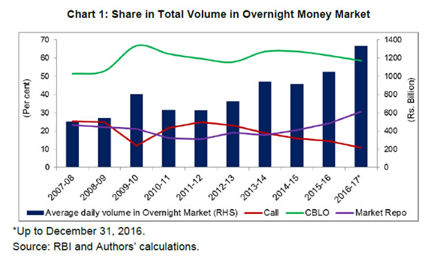

Interest rates in collateralised segment (i.e. CBLO and market repo) should generally be lower than call money rate simply by virtue of these markets being collateralized. This would provide a potential arbitrage opportunity to those who have excess collaterals to borrow from CBLO/ market repo and lend in call money market. However, it has been observed that the collateralised overnight rates (CBLO and market repo) were generally higher than the WACR in the last few years, especially during 2014-15 and 2015-16 (Table 1). It is noteworthy that these overnight rates have converged, on an average basis, during 2016-17 (up to December 31). The existence of higher collateralized rate vis-a-vis uncollateralized rate indicates some kind of infirmities/ frictions in the overnight money market, which may be hampering arbitrage between these two segments, resulting in sub-optimal outcome.

As a major part of the overnight funding from the market is met by CBLO, it could pose a challenge for monetary policy transmission if CBLO rate is not synchronized with call money rate (operating target). An analysis of synchronization among various segments of the overnight money market shows that synchronization between call money and other overnight segments (i.e. CBLO and market repo), as reflected by correlation between cyclical components³ of respective interest rates, witnessed significant improvement and remained at elevated level before weakening in 2015-16 (Table 2).

The synchronisation among overnight segments has also been analysed by estimating GARCH conditional volatility of respective overnight rates. It could be seen in Chart 2 that co-movements among call rate, CBLO rate and market repo rate have generally been synchronized. Improved synchronization among call money and CBLO rates may suggest increased arbitrage between these markets. Although CBLO has wider participation (i.e. entities other than banks are also permitted to participate), banks, which have exclusivity in call money along with primary dealers (PDs), continue to contribute major share in CBLO segment, especially on the borrowing side. The high share of banks in borrowing from CBLO segment may suggest that they may be using part of this borrowing for lending in call money market in order to exploit the arbitrage opportunity, if any.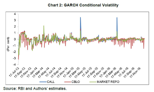

It is clear from the above that the structure of the overnight money market is tilted towards the collaterised segments where a larger part of the overnight funding takes place. This could pose a challenge for monetary policy transmission, which targets uncollateralised inter-bank overnight rate (i.e. WACR). Nonetheless, the above analysis clearly indicates that both uncollaterised and collateralised overnights rates have moved in sync in the last few years, which may be mitigating the above-mentioned concern to a large extent.

Further, the new liquidity management framework, which entails far-reaching changes in the liquidity support provided by the RBI under LAF, has been devised for operationalising monetary policy framework effectively, i.e., to properly align the operating target (WACR) with the policy rate (repo rate). A comparative analysis of movements in WACR and its spread over repo rate during the old liquidity management framework (LMF) and the new LMF has been provided in Table 3 below. It is evident from the table that the spread over the policy rate as well as volatility in the WACR were quite low during the old LMF, represented by the period April 1 2012 to July 16, 2013, as compared to new LMF. Evidently, availability of unlimited liquidity at a fixed rate (repo rate) and greater flexibility in reserve maintenance requirement (minimum 70 per cent of the required reserves on any day during the cycle) led to low spread and less volatility but also stymied the development of the money market, especially the term segment, as unlimited availability of liquidity from RBI under LAF ensured that the RBI became the preferred counterparty. However, against the backdrop of intense volatility in the domestic foreign exchange market with the Indian rupee coming under significant depreciation pressure during the taper tantrums episode of 2013, far-reaching changes were introduced in RBI’s liquidity management operations during July-October 2013. Those, inter alia, included making Marginal Standing Facility (MSF) rate as de facto policy rate, restricting amount available through fixed rate repo, introduction of variable rate term repos, sharp increase in daily reserve maintenance requirement, etc. (Box). These changes led to a sharp increase in both spread and volatility of WACR during sub-period 1 of the transition period as evident from the Table 3. However, with the restoration of orderly conditions in the forex market, phased normalization of monetary policy was carried out during sub-period 2 of the transition phase (October 2013 to March 2014) leading to sharp decline in both spread and volatility of WACR.

Box: New Liquidity Management Framework

• Liquidity from RBI under LAF was restricted to 1.0 per cent of NDTL from July 17, 2013, which was reduced to 0.50 per cent of each bank’s NDTL from July 24, 2013.

• Interest rate on Marginal Standing Facility (MSF) was increased by 200 basis points from July 15, 2013 expanding the upper corridor over repo rate to 300 basis points, which was normalised to 100 basis points by adjusting both repo rate and MSF rate from October 29, 2013. During this period, MSF rate became effective policy rate with significant reduction in availability of liquidity from the Central Bank and tight daily reserve maintenance requirement.

• Additional liquidity equivalent to 0.25 per cent of NDTL of the banking system was made available through 7 days and 14 days repos through variable rate auction each Friday beginning October 11, 2013, which was subsequently increased to 0.50 per cent of the banking system’s NDTL from October 29, 2013.

• With effect from April 1, 2014, the liquidity through fixed rate repo was reduced from 0.50 per cent to 0.25 per cent of each bank’s NDTL and at the same time, the liquidity through 7 days and 14 days variable rate repo was increased from 0.50 per cent to 0.75 per cent of banking system’s NDTL.

• Liquidity framework was again revised from Sept 5, 2014 which entailed provision of liquidity equivalent to one-fourth of the 0.75 per cent of system’s NDTL through 7 days and 14 days variable rate repo auctions every week on Tuesday and Friday. Furthermore, liquidity injection/ absorption through variable rate repo/ reverse repo of various tenors has also been introduced for fine tuning purpose and amount has to be decided based on the assessment of the liquidity conditions. Under the revised framework also, the assured liquidity support from RBI is restricted to 1.0 per cent of banking system’s NDTL.

• Minimum daily reserve maintenance by scheduled commercial banks (SCBs) was increased from 70 per cent to 99 per cent of the requirement effective from July 27, 2013, but it was reduced to 95 per cent from September 21, 2013 and to 90 per cent from April 16, 2016.

Subsequently, with a view to improving the alignment of WACR with the policy rate for more efficient transmission of monetary policy signals and also for developing term money market, based on the recommendations of the Expert Committee to Revise and Strengthen the Monetary Policy Framework, further revisions to NLMF were carried out on September 5, 2014, which, inter alia, included proactive use of variable rate repos/reverse repos of various tenors, four 14 days variable rate term repo auctions equivalent to 0.75 per cent of banking system’s NDTL during a fortnight, use of overnight fine tuning liquidity operations, etc. The liquidity management framework was further revised in April 2016 as the reserve maintenance requirement was further relaxed and RBI decided to shift the system from a position of liquidity deficit to a position closer to neutrality through injection of durable liquidity using open market operations (OMOs). All these changes in NLMF have had a salutary effect on both spread and volatility of the WACR, which have declined sharply and have come closer to the levels witnessed during the old LMF.

IV. Determinants of Call Money Spread: Theoretical Underpinning

As explained in the introduction, factors affecting the call money spread could be derived taking into account both demand and supply of liquidity. These factors have been identified based on the extant literature on the subject (such as, Kucuk, et al., 2014; Linzet and Scvhmidt, 2008; Moschitz, 2004: Beirne, J., 2012) and, at the same time, keeping in view domestic conditions, especially market structure and monetary policy operating framework, etc. The factors identified are liquidity related (viz. liquidity conditions, liquidity uncertainty, liquidity distribution, demand for reserve maintenance and interest rate expectations) and dummy variables representing structural changes and some recurring phenomenon with regard to liquidity requirement. The explanation of these factors affecting the call money spread has been set out in the subsequent paragraphs.

Liquidity factors

The demand for liquidity (reserves) by the banks and supply of liquidity by the central bank determine the liquidity conditions on a particular day. The central bank supplies liquidity to the banks enabling them to fulfill their reserve requirement at interest rate consistent with policy rate. As long as liquidity deficiency (demand) is equal to the supply of liquidity, i.e., there is no liquidity mismatch; the inter-bank rate is closely aligned with the policy rate. The banks are, however, exposed to the unforeseen liquidity shocks, especially at the end of the day, and these shocks force banks to resort to the standing facilities, eventually resulting in deviation of inter-bank rate from the policy rate. In fact, these unforeseen liquidity shocks constitute the core of liquidity condition that moves the inter-bank rate the most. Neyer and Wiemers (2004) present a model market wherein the resulting positive spread between the inter-bank market rate and the central bank rate is determined, inter alia, by total liquidity needs of the banking sector, costs of obtaining funds from the central bank, and the distribution of the latter across banks.

The Reserve Bank provides liquidity through LAF, outright open market operations (OMOs) and various refinance facilities. The outright OMOs are undertaken generally to address the permanent/ structural liquidity deficit, whereas liquidity operations under LAF are targeted to deal with temporary or frictional liquidity deficit in the system. As liquidity under overnight repo was restricted to 0.25 per cent of NDTL, term repos were introduced in October 2013. The changes in autonomous liquidity factors (mainly currency in circulation and Government cash balances) coupled with discretionary policy actions (such as change in CRR, open market operations, intervention in foreign exchange market, etc.) impact the liquidity conditions. In view of the existing liquidity conditions, the banks avail liquidity under LAF from RBI, i.e. tight liquidity conditions would lead to banks availing higher liquidity under LAF and vice versa. To put it differently, the net liquidity injection through LAF is mainly driven by liquidity conditions generated by autonomous factors and favourable liquidity conditions generated by the above factors may result in lower availing of liquidity by banks under LAF. Hence, the availing of liquidity by banks under LAF reflects the liquidity conditions in the system. The impact of liquidity conditions on overnight rates would depend on the extent of liquidity support extended by the RBI, i.e., increase in liquidity tightness would lead to an increase in overnight rates but the extent of increase would depend on the amount of liquidity made available by the RBI under LAF. Access to unlimited liquidity under LAF at fixed rate may largely negate the impact of liquidity conditions on overnight rates (as was the case before restricting assured liquidity under LAF to 1.0 per cent of NDTL from July 17, 2013). As assured liquidity available from RBI under LAF has been restricted (Box), transmission of tight liquidity conditions to overnight rates has increased leading to higher spread and increased volatility under NLMF though use of variable rate repos/reverse repos of various tenors by the RBI under revised liquidity framework has mitigated the situation to a large extent. Notwithstanding the extent of liquidity provided under LAF, the liquidity tightness would generally lead to hardening of overnight interest rates.

As explained above, liquidity availed by banks under LAF (including MSF and term repos) reflects the liquidity conditions, we have taken ratio of net liquidity provided under LAF (including overnight repo, term repo, reverse repo and MSF) to the required reserve maintenance as indicator of the daily liquidity condition in our empirical analysis. Increase in this ratio would signify tightening of liquidity conditions and would lead to an increase in WACR spread and vice versa. Kucuk, et al. (2014) also use net liquidity deficit as ratio of reserve requirement of the banks as a general indicator of daily aggregate liquidity conditions. On the other hand, Linzert and Schmidt (2008) have defined liquidity supply through a variable liquidity policy as the difference between actual allotment and benchmark allotment of liquidity by the European Central Bank (ECB). In Chart 3, the ratio of net liquidity availed under LAF (including MSF) to the required reserve maintenance and WACR spread have been plotted.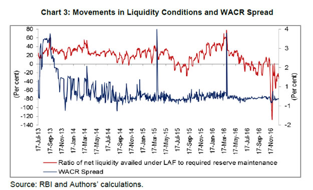

The distribution of liquidity provided by RBI among banks is also likely to impact the call money spread. Under the revised liquidity framework, a major portion of the assured liquidity from RBI is available through variable rate term repo auctions. Theoretically, it means that each bank can potentially corner the entire liquidity auctioned under term repos, provided they have sufficient collaterals available and bid so aggressively that their bid for interest rate is the highest. Notwithstanding the above scenario being just theoretical and almost impossible, under the extant situation, it is possible that a few banks may be successful in securing a large part of the liquidity available under term repos, resulting into lop sided (heterogeneous) distribution of net primary liquidity (which means that some banks secure liquidity more than they require, while others secure less than their requirement).

In other words, some banks may have surplus liquidity while others may have liquidity deficit. The banks having surplus liquidity may try to exploit arbitrage opportunity by lending in overnight segments, including inter-bank call money segment. The arbitrage is necessary for alignment of interest rates among various market segments and for efficient monetary policy transmission. The arbitrage in various segments of debt markets enables transmission of policy rate changes to the long-term interest rates and, hence, the central bank encourages such an arbitrage. A bank which has a liquidity deficit encounters higher uncertainty when it has to borrow from another bank in the overnight market instead of borrowing from the central bank and the uncertainty increases when the borrower bank is unable to gauge the lending condition of the banks with surplus liquidity, i.e., the extent of surplus with the latter. Thus, the skewed distribution of central bank’s liquidity may impact the WACR spread or overnight rates spread adversely, i.e. higher heterogeneity in distribution of central bank liquidity is likely to push the call money spread. Kucuk, et al. (2014) represents liquidity distribution among banks through a ratio of the volume of overnight repo transactions in inter-bank repo-reverse repo market (IRM) to the total volume of overnight transactions.

In this study, we have presumed the ratio of volume in inter-bank call money to the total volume in the overnight market as representative of the distribution of central bank liquidity among banks. This indicator has been taken as proxy of liquidity distribution in our study and has been juxtaposed with WACR spread in Chart 4. It is presumed that homogenous or less heterogeneous distribution of central bank liquidity would meet a large part of liquidity requirement of each bank, reducing their dependence on inter-bank call money market and accordingly, this ratio would be lower. On the other hand, more heterogeneous distribution of liquidity (i.e. few participants cornering large part of liquidity) is likely to result in higher call money market volume and accordingly, this ratio would go up. Therefore, a rise in this ratio is likely to result in increase in WACR spread. The positive relationship between this ratio and WACR spread may also reflect the shallowness of the call money market where few market participants could drive the market.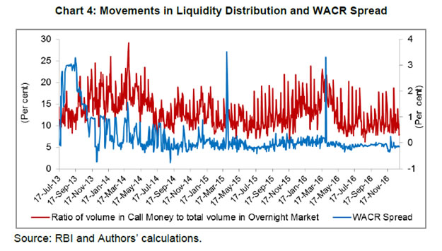

The requirement of short-term funds by banks is largely driven by their reserve requirements. Besides reserve requirements, other factors that may influence the demand for liquidity are interest rate expectations and liquidity uncertainty.

Banks have been allowed daily averaging of reserve maintenance over the reserve maintenance period, i.e., the fortnight, but subject to minimum daily requirement. The averaging for reserve maintenance is allowed across several jurisdictions, e.g., the European Central Bank (ECB) has allowed daily averaging over a maintenance period of six weeks without any daily minimum requirement. One of the objectives of averaging allowed by the ECB is to stabilise money market interest rates. The Federal Reserve also requires banks to maintain reserve on an average over a fortnight, subject to daily maintenance at greater than or equal to the bottom of its penalty-free band (which is reserve balance requirement minus higher of USD 50,000 or 10 per cent of reserve balance requirement).

In India, the daily minimum reserve requirement was enhanced from 70 per cent to 99 per cent on July 27, 2013 but subsequently reduced to 95 per cent from September 21, 2013 and to 90 per cent from April 16, 2016. The banks borrow from the RBI and overnight markets to meet their reserve requirements and for bridging their temporary funding gaps. Therefore, the reserve requirement remains a major driver of demand for daily liquidity and as daily minimum reserve requirement at elevated level constrains the flexibility of banks, this might be creating additional demand pressure for liquidity at times leading to spikes in overnight rates (Chart 5). This component of demand for liquidity could be best explained by the cumulative average reserve fulfillment during the maintenance period, as the extant reserve maintenance allows banks to smooth their reserve fulfillment within the maintenance period. If cumulative average reserve ratio is lower than required, then demand for liquidity for maintaining required reserve ratio is going to be higher during the remaining days of the maintenance period. The reverse may happen if cumulative average reserves fulfillment is higher than required. This higher demand for liquidity would eventually get reflected in an increase in cumulative average reserve ratio and pressure on overnight rates⁴.

Friedman and Kuttner (2010), however, find demand for reserve highly interest-inelastic during the maintenance period with an evidence of an increase in reserve by US$ 1 billion leading to decline in federal fund rate by less than one basis point on any given day. Linzert and Schmidt (2008) and Kucuk, et al. (2014) also capture the banks’ demand for liquidity through cumulated average reserve maintenance.

Against the above backdrop, the relationship between cumulative reserve maintenance ratio with a lag and call money spread is supposed to be negative as higher cumulative average reserve fulfillment would mean lower future reserve pressure. In this paper, the cumulative average of reserve maintenance ratio during the reserve maintenance period with a lag has been taken as representative indicator of demand for reserve (liquidity).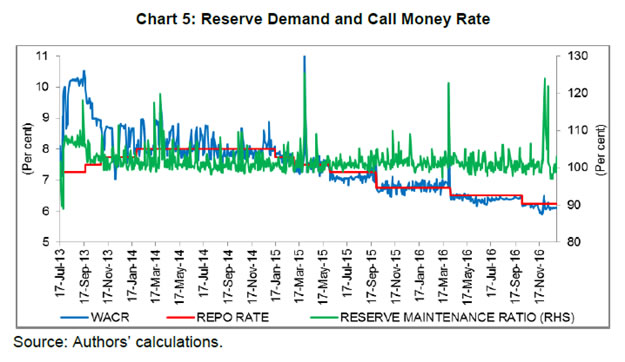

Interest rate expectations also influence demand for short-term liquidity, especially in the backdrop of banks trying to minimise the cost of maintaining required reserves. In order to achieve this cost minimization objective, banks’ demand for current liquidity may go up if they expect that the short-term interest rates will go up during the remaining reserve maintenance period and reverse may happen, if they expect the short-term interest rate to decline. The expected changes in the future short-term interest rate could be on account of expected change in the policy rate or other factors and such changes could be best captured by the forward rate. In the absence of overnight forward rate, longer maturity forward rate may be able to capture the expected changes in overnight rates, as long-term rate is the weighted average of expected short-term rates following the expectation theory of term structure of interest rate. Interest rate futures (IRF) were permitted long back but not much of trading took place until recently when cash settled IRF was permitted on 10 year bonds. Although there has been reasonable trading in 10 year cash settled IRF since December 2013, the same cannot be used as indicator of interest rate expectations in our analysis due to non-availability of data for the entire sample period. However, interest rate swaps (IRS) of 1 year maturity is quite liquid as well as available for longer time period and, hence, these rates could be used to reflect changing interest rate expectations. Both Kucuk (2014) and Linzert and Schmidt (2008) take swap rates as an indicator of interest rate expectations. We also use 1 year IRS as an indicator to represent the interest rate expectations in our analysis (Chart 6). It is presumed that rise in interest rate expectations may lead to increased demand for overnight borrowing for fulfilling reserve maintenance requirement, which, in turn, may result in hardening of overnight spreads including call money spread.

Liquidity uncertainty that may largely stem from supply side may also impact the behavior of banks in the overnight market. Unlimited liquidity made available under LAF earlier had almost eliminated the supply side liquidity uncertainty. The supply side uncertainty, however, appeared when RBI restricted overall liquidity available under LAF. Furthermore, major portion of the restricted liquidity under LAF being made available through variable rate term repos appears to have further reinforced the liquidity uncertainty as this liquidity is offered through variable rate auctions and successful players only get this liquidity. This means that banks are not sure about the amount of liquidity they will be able to get from this pool of liquidity available through variable rate term repos. Further, the banks may be uncertain about the bidding behavior of their competitors and this may be influencing their bidding behavior in the term repo auctions, inducing them to bid aggressively. Given the supply side liquidity uncertainty and uncertainty about the bidding behavior of the banks, overall liquidity uncertainty may be proportional to the demand for liquidity, i.e., increase in demand for liquidity would result in higher liquidity uncertainty. In case of increased liquidity uncertainty, banks may bid aggressively both in term repo and overnight market to corner the liquidity that provides comfort to them, eventually leading to increase in overnight rates. Valimaki (2006) demonstrates that allotment uncertainty can lead to an increasing marginal rate of tender even if banks are being provided sufficient liquidity in principle by the European Central Bank (ECB). Such uncertainty could be captured by bid-cover ratio in term repo auctions, as higher bid-cover ratio would suggest higher liquidity uncertainty. However, term repo auctions started in October 2013 and that too once in a fortnight and only recently (starting from Sept 5, 2014) such auctions are being conducted four times in a fortnight. As number of observations in respect of bid-cover ratio in term-repo auctions is not sufficient to consider in the estimation, the liquidity uncertainty has been derived as conditional variance⁵ (volatility) of cumulative reserve maintenance ratio⁶. One step ahead conditional variance of reserve maintenance ratio would represent the extent of uncertainty about liquidity demand of banks and, hence, uncertainty about their bidding behavior in overnight market and term repo auctions.

Dummy variables

Some autonomous factors, which might be impacting the overnight rates, may be difficult to quantify. Impact of such factors on overnight rates may be captured best by dummy variables. One such factor that could be impacting the demand for overnight liquidity and thereby interest rates may be the banks’ tendency to build up cash balances at the quarter-end mainly for balance sheet management. This means that lendable funds in the overnight market get reduced significantly at the quarter-end due to the banks’ unwillingness to lend, despite having surplus liquidity, leading to spike in overnight interest rates. In order to represent this behavior of banks, we have included a dummy variable (DUM1) by assigning value 1 for each quarter-end in the analysis. The liquidity management framework underwent major changes with liquidity under LAF being restricted, substantial increase in the MSF rate and significant increase in daily minimum reserve maintenance in July 2013 in the wake of the taper tantrums episode (Box). Most of these changes in the liquidity management framework were normalized by end-October 2013 but some of them continued and assumed structural nature. These changes appear to have reduced flexibility and increased banks’ demand for overnight liquidity impacting the overnight spread adversely. Thus, the changes which were normalized by end-October 2013 have been captured by introducing a dummy variable (DUM2) in the analysis by taking value 1 for each day from July 17, 2013 to October 28, 2013 and zero for other days. Another important change in the liquidity management framework during the study period was the introduction of fine turning liquidity management operation with variable rate reverse repo and repo auctions of various tenors from September 5, 2014. The fine-tuning operations have helped to deal with liquidity shocks generated by various autonomous factors and, at the same time, reduced liquidity uncertainty, eventually enhancing the alignment of the WACR with the policy rate. We have captured this change in our analysis by including a dummy variable (DUM3) by taking value one for each day from September 5, 2014 onwards. We have included a total of three dummy variables to capture various changes in the liquidity management framework undertaken during our study period.

V. Data and Methodology

Data

We have used daily data from July 17, 2013 to December 31, 2016 as the objective of our study is to analyse the factors driving the WACR spread under the NLMF. Since trading volumes in the call money on Saturdays remain very low due to large part of financial sector being closed on that day, this day has been excluded from our analysis. We have taken the following variables in our study: (a) call money rate spread (CALLSP); (b) liquidity conditions (LQDCD); (c) liquidity distribution (LQDIST); (d) demand for reserve (DRES); (e) liquidity uncertainty (LQUNCERT); (f) interest rate expectations (IEXP); (g) dummy for changes in liquidity management framework and minimum reserve maintenance on the back of taper tantrum (DUM1); (h) dummy for banks’ tendency to build up cash balances at the quarter-end for balance-sheet window dressing (DUM2); (i) and dummy for fine tuning operations started from September 5, 2014 (DUM3). The variables’ description along with their expected influence on call money rate spread is given in Table 4 below.

Table 5 above contains descriptive statistics of variables taken into empirical exercise and it is found, based on both Skewness and Kurtosis, that these variables are not normally distributed. Further, all variables, except for interest rate expectations, are leptokurtic as Kurtosis is higher than the threshold value of three.

Methodology

Augmented Dickey-Fuller (ADF) and the Phillips-Perron (PP) tests have been used to test the mean reverting (stationary) property of variables. The ADF test applies parametric transformation by adding the lagged values of the dependent variable (which is in difference form) to eliminate the serial correlation in the error terms. The numbers of lagged difference terms are included empirically so that error terms become serially uncorrelated. On the other hand, the PP test uses nonparametric statistical methods to address the serial correlation in error terms without adding lagged difference terms.

Simple ordinary least square (OLS) can be used to estimate the relationship between dependent variable (CALLSP) and explanatory variables. Linzert and Schmidt (2008) and Kucuk, et al. (2014) have also used OLS regression on daily data to explain the overnight spread. However, the estimation of OLS regression with high frequency data is generally beset with the problem of presence of autocorrelation, suggesting problem of “autocorrelation in volatility”. This requires testing for ARCH effects as standard errors become biased and inconsistent in the presence of such effects resulting in heteroscedasticity problem. Recent innovation in this field by Whitney and Ken West (1987), known as “The Newey-West heteroskedasticity and serial correlation consistent standard errors”, however, allows quite a good estimate of standard errors in the presence of heteroskedasticity and serial correlation. As ARCH effect is found to be present, we have also used the Newey-West heteroskedasticity and serial correlation consistent variance estimator. Our basic OLS equation has the following expression:

We have also augmented OLS equation by GARCH models for correcting ARCH errors and for corroborating the results of the above OLS equation. We use three variants of GARCH models, viz., parsimonious GARCH, integrated GARCH (IGARCH) and exponential GARCH (EGARCH) for robustness check and for capturing the volatility appropriately. IGARCH model captures the persistence in variance, while EGARCH captures the asymmetric effect in volatility. The GARCH models are non-linear and, therefore, are estimated via maximum likelihood.

It has been observed in the literature that the specifications of conditional covariance matrix contain a large number of parameters which along with positive definite condition make the Quasi-Maximum Likelihood (QML) method quite difficult to apply for estimation (Francq et al., 2014). As a consequence, the variance targeting estimation (VTE), propounded by Engle and Mezrich (1996), has become very prominent in the studies involving high frequency financial series. Francq et al., (2009) underline that the potential benefits of VTE may not be limited only to the numerical optimization but this procedure also ensures that the GARCH estimates of unconditional variance is equal to the sample variance⁷. We also use VTE for GARCH (1,1) and the variance equation of our basic GARCH (1,1) model has the following expression:

It is often found that the sum of the estimated parameters in the standard first-order GARCH model (p=q=1) is close to unity suggesting “persistent variance”. In these kinds of models, the current information remains pivotal and plays an important role in forecasting of conditional variance. This phenomenon was first noticed by Engle and Bollerslev (1986) and they suggested imposing of restriction on parameters α₁+ α₂ = 1 and termed such a model as integrated GARCH (IGARCH). The IGARCH process is not weakly stationary but strongly stationary, however, sometimes this integrated term, which is generally associated with unit root in modeling, may be somewhat misleading (Terasvirta, 2006). With the above parametric restriction, the variance equation with IGARCH will have the following expression:

EGARCH, introduced by Nelson (1991), is another popular model which deals with the limitations of the standard GARCH models. GARCH models assume that volatility is determined only by the magnitude and not by the positivity or negativity of unanticipated excess returns. Another limitation of GARCH models is non-negativity constraints on parameters in variance equation. First, EGARCH model does not require any parameter restrictions to ensure positive conditional variance at all points and second, this model captures the asymmetric effect of shocks on volatility. EGARCH is first asymmetric model wherein variance is dependent on both the size and the sign of lagged residuals. The variance equation (3) in EGARCH is as under:

As liquidity conditions, demand for reserves and quarter-end phenomenon are already known to impact the call rate spread, these variables in the mean equation have been taken as control variables in order to gauge the impact of other variables on the call rate spread.

VI. Empirical Findings

The results of unit root test are furnished in (Appendix Table 1) and except for interest rate expectation (IEXP), all variables are found to be stationary. IEXP is, however, found to be stationary in first difference and, accordingly, we have used it in first difference in our estimation. In order to see prima facie relationship between dependent variable and explanatory variables, we have computed simple correlations and the results are furnished in Appendix Table 2. The results display some relationship between call money spread (CALLSP) and explanatory variables, i.e. liquidity conditions (LQDCD), demand for reserve (DRES), liquidity uncertainty (LQUNCERT) and interest rate expectations (IEX). Before estimating final relationship, we have tested for structural breaks on specific points with Chow Breakpoint test. The results of Chow Breakpoint test, furnished in Appendix Table 3, suggest presence of structural break on October 28, 2013 and September 5, 2014 and justify inclusion of DUM2 and DUM3 in our estimation. Appendix Table 4 presents the result of tests for the presence of serial correlation and Heteroskedasticity in estimation of equation (1) with simple OLS. We have found presence of serial correlation and Arch effects (Heteroskedasticity) in the residuals. In the presence of serial correlation and Heteroskedasticity, we have estimated OLS with HAC standard errors & covariance, as suggested by Whitney and Ken West (1987) and the results are furnished in Appendix Tables 5 and 6. The results of GARCH models, estimated to corroborate the results of OLS model and also to completely remove the heteroskedasticity problem, are given in Appendix Tables 7 and 8. We have also estimated both OLS with HAC standard errors & covariance and GARCH models for two sub-periods in order to see the impact of certain variables, such as, LQUNCERT on CALLSP after introduction of fine tuning liquidity management operation with effect from September 5, 2014.

In both types of models, the coefficients of liquidity conditions (LQDCD), liquidity distribution (LQDIST), liquidity uncertainty (LQUNCERT) and dummy variables (DUM1, DUM2, and DUM3) are found to be statistically significant and having expected sign. The liquidity conditions (LQDCD) have been found impacting the call money spread (CALLSP) positively, i.e. tightening of liquidity conditions increases call money spread. This result supports the underlying hypothesis as well as the existing research findings (such as, Kucuk, et al, 2014; Linzert and Schmidt, 2008; Moschitz, 2004). The distribution of liquidity (LQDIST) has been found having positive influence on call money spread (CALLSP), which means that increased skewness in the distribution of central bank’s liquidity among banks drives up call money spread. This finding is also in line with the underlying hypothesis and the findings of various cross-country studies. The size of the coefficients on both LQDCD and LQDIST is, however, very small, suggesting marksmanship in liquidity management by the RBI. The liquidity uncertainty (LQUNCERT), estimated in terms of conditional variance of the cumulative average of reserve maintenance ratio during the fortnight, drives up the call money spread. The channel through which this factor operates is bidding behavior of banks in the repo auctions conducted by the RBI under LAF as well as in the call money market, which tends to become aggressive with increased liquidity uncertainty. It is noteworthy that although liquidity uncertainty has been found impacting the call money spread during both sub-periods, the size of the coefficient of LQUNCERT drops during sub-period 2, suggesting moderation in liquidity uncertainty on the back of fine tuning liquidity management operations introduced during this period.

The dummy variable (DUM1), representing quarter-end phenomenon, has been found impacting the call money spread (CALLSP) adversely, i.e., quarter-end build up of cash balances by banks drives up call money spread. This kind of behavior is observed almost every quarter-end when liquidity becomes a scarce commodity due to banks’ unwillingness to part with surplus funds. The impact of structural changes in liquidity management framework, which has been captured through a dummy (DUM2), on call money spread (CALLSP) has been found positive and quite strong. These changes led to steep rise in call money spread, which was also the target in order to deal with taper tantrum spillovers to exchange rate. Another dummy (DUM3), representing fine tuning liquidity management operations with effect from September 5, 2014, has been found easing call money spread (i.e. fine tuning liquidity management operations reduces call money spread (CALLSP)). These changes in liquidity management framework were aimed at meeting evolving liquidity requirements of the banking system in a proactive manner.

The coefficient of demand for reserves (DRES) with a lag has, however, been found to be statistically insignificant in all models. This result suggests that increase in demand for liquidity for reserve maintenance does not impact the call money spread (CALLSP). We may interpret this result by inferring that liquidity management by the central bank is sufficient for the banks to be able to meet their daily reserve requirements without much pressure.

VII. Conclusion

We have attempted to empirically investigate the impact of possible determinants, identified based on the extant literature and domestic framework, on the WACR spread over policy rate to draw some policy inferences. The liquidity conditions have been found driving up the WACR spread, i.e. tightening of liquidity conditions lead to hardening of WACR. Similarly, the skewed distribution of liquidity has been found impacting the call money spread adversely. The impact of both liquidity conditions and liquidity distribution has, however, been found to be very small, reflecting marksmanship in liquidity management by the central bank. Another important factor that has been found affecting the call money spread is liquidity uncertainty, i.e., increase in liquidity uncertainty leads to rise in call money spread. Potential liquidity uncertainty may have gone up with a large part of the central bank’s liquidity being offered through variable rate repos under the new liquidity management framework. Liquidity uncertainty, however, appears to have come down with the introduction of fine tuning operations with effect from September 5, 2014 and, accordingly, its impact on call money spread has moderated. In fact, these fine tuning liquidity management operations aimed at proactively meeting evolving systemic liquidity requirements, captured in our model through a dummy variable, have been found to be reducing the call money spread. During the period of our study, the average of absolute WACR spread (excluding Saturdays) has come down substantially from 85 basis points during pre fine tuning operations period to about 13 basis points in the post fine tuning operations period. Banks’ reluctance to part with surplus funds at the quarter end due to regulatory/ balance sheet consideration, known as quarter-end phenomenon and captured in our study through a dummy variable, is found to impact the call money spread adversely.

In light of the above, some policy actions may help in improving further the alignment of call money rate with the policy rate. Already RBI has taken a number of steps like more proactive use of variable rate repos and reverse repos of various tenors for better liquidity management to keep the rates aligned with the policy rate, reducing the minimum daily reserve requirement from 95 per cent to 90 per cent, bringing the liquidity deficit in the system closer to neutrality through OMO purchase auctions and narrowing of the policy rate corridor to +/- 25 basis points very recently. Greater flexibility in averaging the reserve maintenance during the maintenance period may, however, further reduce the stress on overnight liquidity and, eventually, may help in bringing down the liquidity uncertainty. Internationally, some jurisdictions also allow averaging of reserve maintenance without any minimum daily requirement (e.g. European Central Bank (ECB) allows daily averaging over a maintenance period of six weeks without any daily minimum requirement). One of the objectives of averaging allowed by the ECB is to stabilise money market interest rates. The Federal Reserve also requires banks to maintain reserve on an average over a fortnight, subject to daily maintenance at greater than or equal to the bottom of its penalty-free band. Besides, the recent narrowing of policy rate corridor is expected to reduce the volatility in the WACR and improve the alignment of the WACR with the policy rate, thereby improving monetary transmission. There is also a need to have greater alignment between various money market rates for more efficient transmission of the monetary policy signals. In this context, frictional elements like persistently higher rates in market repo segment vis-a-vis the call money segment, despite the former being collateralized, also need to be addressed.

^@ Sunil Kumar is a Director in the Department of Economic and Policy Research and Anand Prakash is a Director and Krishna M Kushawaha is an Assistant Adviser in the Financial Markets Operations Department of the Reserve Bank of India.

¹ Authors are grateful to Shri Dipankar Biswas, Dr. Susan Thomas, Shri Sitikantha Pattanaik, Shri Bhupal Singh, Shri Indranil Bhattacharyya, and Shri Rajesh Kavediya for offering useful comments and suggestions on an earlier version of the paper. The views and opinions expressed in this paper are strictly those of the authors and do not represent the views of the RBI in anyway.

^[1] The Central Government, in consultation with the Reserve Bank, has notified the inflation target of 4+/-2 per cent (with 6 per cent and 2 per cent as upper limit and lower limit, respectively) on August 5, 2016. This inflation target is applicable for the period from August 5, 2016 to March, 2021 (RBI, 2016).

^[2] Naturally, the more comprehensive is the central banks model of the overnight rate, the more it will actually be able to identify the adequate policy measure in order to control it to the possible and desired extent (Wurtz, F.R. (2003)

^[3] Cochrane (2001) elaborates lucidly the expectation hypothesis and model for term-structure of interest rates.

^[4] The central bank could influence supply side strongly but may not be able to control it perfectly (Moschitz, Julius, 2004).

³ The cyclical component of interest rates has been separated from their trends by using Hodrick–Prescott filter.

⁴ On the contrary, Patra et al. (2016) in this regard argues that reserve averaging procedures, lagged reserve maintenance periods and standing facilities render banks’ demand for reserves interest elastics on a day-to-day basis, but inelastic on a longer term basis.

⁵ The conditional variance is one period ahead forecast variance based on past information.

⁶ Linzert and Schmidt (2008) also capture liquidity uncertainty with the conditional volatility from cumulated average reserve fulfilment during a maintenance period. On the other hand, Kucuk, et al. (2014) take the ratio of the expected intra-day cash flows to the amount of reserves balances at the beginning of the day to capture the information on funding (liquidity) uncertainty.

⁷ Francq, et al., (2009) further highlight that it is possible that in a case of misspecification, i.e., when the true underlying process is not a GARCH, the approximation provided by the VTE is superior, in some sense, to that obtained by QMLE.

References:

Bartolini, L., G. Bertola and A. Prati (2000), ';Day-to-day Monetary Policy and the Volatility of the Federal Funds Interest Rate';, Working paper WP/00/206, IMF.

Bech, M. and C. Monnet (2013), “The Impact of Unconventional Monetary Policies on the Overnight Interbank Market”, Reserve Bank of Australia Conference, Volume 2013.

Beirne, J. (2012), “The EONIA Spread Before and During the Crisis of 2007–2009: The Role of Liquidity and Credit Risk”, Journal of International Money and Finance, Volume 31, Issue 3, pages 534-551

Binici, M., H. Erol, H. Kara, P. Özlü and D. Ünalmış (2013), “Interest Rate Corridor: A New Macroprudential Tool?” CBRT Economic Note, No: 13/20.

Brunetti, C., M. di Filippo and J.H. Harris (2011), “Effects of Central Bank Intervention on the Interbank Market during the Sub-Prime Crisis”, The Review of Financial Studies, Vol. 24, No. 6, pages 2053-2083.

Christensen, J. H. E., J. A. Lopez and G. D. Rudebusch (2009), ';Do Central Bank Liquidity Facilities Affect Interbank Lending Rates?'; Working paper 2009-13, Federal Reserve Bank of San Francisco.

Eisenschmidt, J., A. Hirsch and T. Linzert (2009), ';Bidding Behaviour in the ECB’s Main Refinancing Operations during the Financial Crisis';, Working Paper 1052, ECB.

Engle, R.F. and J. Mezrich (1996), “GARCH for groups”, Risk 9, 36–40.

Francq, C., L. Horvath and J.M. Zakoian (2009), “Merits and drawbacks of variance targeting in GARCH models”, MPRA Paper No. 15143, posted 9. May 2009 at http://mpra.ub.uni-muenchen.de/15143/

Francq, C., L. Horvath and J.M. Zakoian (2014), “Variance targeting estimation of multivariate GARCH models”, MPRA Paper No. 57794, posted 6. August 2014 at http://mpra.ub.uni-muenchen.de/57794/

Friedman, B. M. and K. N. Kuttner (2010), ';Implementation of Monetary Policy: How Do Central Banks Set Interest Rates?'; Working paper, 16165, NBER.

Gaspar, V., G. Perez-Quirós and H.R. Mendizábal (2004), ';Interest Rate Determination in the Interbank Market';, Working Paper, 351, ECB.

Ghosh, S. and I. Bhattacharyya (2009), “Spread, Volatility and monetary policy: empirical evidence from the Indian overnight money market”, Macroeconomics and Finance in Emerging Market Economies, 2:2, 257-277.

Government of India (2015), “Agreement on Monetary Policy Framework between the Government of India and the Reserve Bank of India”.

Hassler, U. and D. Nautz (2008), “On the Persistence of the Eonia Spread”, Economics Letters, Volume No 101, Issue 3, pages 184-187

Joyce, M., A. Lasaosa, I. Stevens and M. Tong (2011), “The Financial Market Impact of Quantitative Easing in the United Kingdom”, International Journal of Central Banking, September 2011.

Krishnamurthy, A. and A. Vissing-Jorgensen (2011), “The Effects of Quantitative Easing on Interest Rates: Channels and Implications for Policy”, Brookings Papers on Economic Activity, Fall 2011.

Kucuk, H., P. Ozlu, A. Talasli, D. Unalmis, and Canan Yuksel (2014), “Interest Rate Corridor, Liquidity Management and the Overnight Spread”, Working Paper No: 14/02, Central Bank of the Republic of Turkey.

Linzert, T., and S. Schmidt (2008), “What Explains the Spread between the Euro Overnight Rate and the ECB’s Policy Rate?” Working Paper Series No. 983/ December 2008, European Central Bank.

Moschitz, J. (2004), “The Determinants of the Overnight Interest rate in the Euro Area”, Working Paper Series No. 393/ September 2004, European Central Bank.

Nautz, D. and C.J. Offermanns (2006), ';The Dynamic Relationship between the Euro Overnight Rate, the ECB.s Policy Rate and the Term Spread';, Working Paper, 01/2006, Deutsche Bundesbank.

Nelson, D. B. (1991), ';Conditional Heteroskedasticity in Asset Returns: A new approach';, Econometrica, 592, 347.370.

Neyer, U. and J. Wiemers (2004), “The Influence of a Heterogeneous Banking Sector on the Interbank Market Rate in the Euro Area”, Swiss Journal of Economics and Statistics (SJES), vol. 140, issue III, pages 395-428.

Nobili, S. (2009), ';Liquidity risk in money market spreads';, paper presented at ECB Workshop on ‘Challenges to Monetary Policy Implementation beyond the Financial Market Turbulence’, Frankfurt.

Patra, M.D., M. Kapur, R. Kavediya, and S.M. Lokare (2016), “Liquidity Management and Monetary Policy: From Corridor Play to Marksmanship”, in C. Ghate and K.M. Kletzer (eds.), Monetary Policy in India: A Modern Macroeconomic Perspective, Springer India.

Perez-Quirós, G. and H.R. Mendizábal (2006), ';The Daily Market for Funds in Europe: What has Changed with the EMU?'; Journal of Money, Credit, and Banking, 381, 91.118.

RBI (2016), “Annual Report 2015-16”.

RBI (2014), “Report of the Expert Committee to Revise and Strengthen the Monetary Policy Framework” (Chairman: Urjit R. Patel).

RBI (2011), “Report of the Working Group on Operating Procedure of Monetary Policy” (Chairman: Deepak Mohanty).

Soares, C., P.M.M. Rodrigues (2011), “Determinants of the Econia Spread and the Financial Crisis”, Working Papers, 12/2011. Banco de Portugal.

Szczerbowicz, U. (2011), “Are Unconventional Monetary Policies Effective?” CeLEG Working Paper, No: 07.

Szczerbowicz, U. (2012), “The ECB Unconventional Monetary Policies: Have They Lowered Market Borrowing Costs for Banks and Governments?” CEPII Working Paper, No: 2012-36.

Terasvirta, T. (2006), “An Introduction to Univariate GARCH Models”, SSE/EFI Working Papers in Economics and Finance, No. 646.

Välimäki, T. (2008), ';Why the Effective Price for Money Exceeds the Policy Rate in the ECB Tenders? Working Paper 981, ECB.

Valimaki, Tuomas (2006), “Why the Marginal MRO Rate Exceeds the ECB Policy Rate”. Bank of Finland Research Discussion Papers, 20, 2006.

Whitesell, W. (2006), “Interest Rate Corridors and Reserves”, Journal of Monetary Economics, 53, 1177–1195.

Wurtz, F. R. (2003), “A Comprehensive Model of the Euro Overnight Rate';, Working Paper 207, ECB.