by
A. Ganesh-Kumar1
Bipul K Ghosh
Khaijamang Mate
Prayag Singh Rawat
Issued for Discussion DRG Studies Series Development Research Group (DRG) has been constituted in Reserve Bank of India in its Department of Economic and Policy Research. Its objective is to undertake quick and effective policy-oriented research backed by strong analytical and empirical basis, on subjects of current interest. The DRG studies are the outcome of collaborative efforts between experts from outside Reserve Bank of India and the pool of research talent within the Bank. These studies are released for wider circulation with a view to generating constructive discussion among the professional economists and policy makers. Responsibility for the views expressed and for the accuracy of statements contained in the contributions rests with the author(s). There is no objection to the material published herein being reproduced, provided an acknowledgement for the source is made. DRG Studies are published in RBI web site only and no printed copies will be made available. Director
Development Research Group |
Acknowledgement The authors are deeply grateful to Dr. M.D. Patra, Executive Director, Reserve Bank of India for his constant support/encouragement to complete the study. We are also thankful to Dr. Rajiv Ranjan, Adviser, Department of Economic and Policy Research (DEPR) for his valuable guidance and support. We thank Dr. Satyananda Sahoo, Director, DEPR and his team members for their constant support and suggestions at each stages. The authors would also like to thank the participants at the various meetings held at the DEPR for their comments and suggestions, including on a set of preliminary results that were presented at the DEPR, which has helped shape the scope of this study and refine the analysis carried out here. The authors would also like to thank an anonymous referee for the insightful comments on an earlier draft, which have helped improve the report. Needless to say, the views expressed here are those of the authors alone and not of the Institutions to which they belong or of the FSU/DEPR/ RBI or the participants in the various meetings held at the DEPR or of the referee.
Executive Summary In this study, we examine the impacts of various types of government expenditure on the Indian economy. In particular, we examine the impacts of a rise in (a) Government consumption expenditure in general and the nature of the relation between government expenditure and GDP, (b) Government expenditure in Social Sectors and in Public Administration, (c) Government transfer payments to households, and (d) Public investment. Towards this, we have used a recursively dynamic computable general equilibrium (CGE) model of the Indian economy developed by Bhakta and Ganesh-Kumar (2016), which is built around a social accounting matrix (SAM) for the year 2011-12. The SAM and the model distinguish 9 commodities/ sectors, 9 factors of production, and 12 household types distinguished by their location and by the monthly per capita expenditure (MPCE) percentile. The model is solved annually over the period 2011-12 to 2025-26. As a first step, we develop a BASE scenario that captures a “Business As Usual” trajectory that the Indian economy is likely to take over the 10-year period 2016-17 to 2025-26 given the current structural characteristics of the economy, and the set of policies currently prevailing. We then develop five sets of counter-factual policy scenarios to study the economy-wide impacts of different types of public expenditure. Each of these sets consists of two or more simulations that are designed to address one main question and its sub-questions, if any. The impacts in each simulation are assessed by comparing the model outcomes in that simulation with the BASE scenario. Our results show that the impact of expansion in government expenditure across different types of expenditure depends crucially on the prevailing macroeconomic conditions, especially whether there is full employment/ unemployment of factors, and also on the complementary set of policies that are needed to generate the resources required to finance the additional expenditure. The main messages that emerge are as follows: -
Fiscal expansion in boom times is actually disastrous for the economy on all counts. -
However, it is not a foregone conclusion that fiscal expansion during recessionary conditions when unemployment prevails is always beneficial. It depends crucially on the type of government expenditure undertaken and the accompanying set of policies that determine how fiscal expansion is financed. -
Amongst alternative types of current expenditure, clearly expansion of government consumption scores over additional transfers to households in terms of impact on GDP. -
Between additional government current consumption and investment, the choice is not straightforward. -
Using additional taxes on households to finance expansion of public investment does not fare well compared to government consumption. -
Nor does shifting of government expenditure from current consumption to investment help if the exchange rate regime is neutral. -
Amongst all the policy options considered in this study, shifting of government expenditure from current consumption to investments accompanied by a slight depreciation of the Rupee turns out to be the best in terms of overall impacts on the GDP and various other macro indicators as well as household real income per capita.
Some Macroeconomic Impacts
of Different Types of Public Expenditure in India -
Analysis Using a Computable General Equilibrium Model Introduction High fiscal deficit, driven by a combination of large government expenditure towards current consumption, very high levels of subsidies, and low (direct) tax base have been an enduring feature of the fiscal situation in India, especially since the onset of the global economy crisis in 2008. In contrast, government investment, particularly in infrastructure and social sectors, has not kept pace with the demand for the services of these sectors. This has resulted in several and severe supply bottlenecks in key sectors such as electricity, transport, etc., with cascading impact on other sectors and the economy in general. In recent years, significant progress has been made to bring down the fiscal deficit and there are early signs that the process of fiscal consolidation is possibly having the desired effects on key macroeconomic variables such as GDP growth and inflation. Even as the government undertakes measures for fiscal consolidation, there is no denying that public current expenditure and public investments will continue to play a significant role in the evolution of the economy in the foreseeable future. Indeed, one prevailing view is that public expenditure, especially investments, in key sectors such as infrastructure (electricity, transport, etc.), social sectors (education and health), and agriculture are grossly inadequate to meet the needs of the economy/ society. Proponents of this view call for a massive ramping up of public expenditure in these sectors given the important role that they play in reducing poverty and improving living standards, food and nutritional security, and in overall human development. In recent years, voices in support for increasing public expenditure has also come about following the sharp slowdown in the growth performance of the country and the slow recovery witnessed thereafter. The general stance here is that public expenditure can expand aggregate demand, which in turn can help revive private investment sentiments, and thus facilitate the return of the economy to a high growth trajectory. Even as there is some merit in these arguments, one should recognise that public expenditure can also have some negative effects. Excessive public expenditure/ very high fiscal deficit can be inflationary, especially if accompanied by monetary accommodation. High fiscal deficit would mean that government would be competing for a larger portion of resources. And if the relative efficiency of public sector is lower than private sector, as is often the case, then it would imply that the overall efficiency of the economy in putting best use of its resources remains rather low. Given these two sides to the nature of public expenditure, in order to make informed policy decisions on public expenditure – how much, in which sector(s), should it be current or capital, should the government spend it by itself or transfer the resources to households – it is then critical to understand the effects of various types of public expenditure. Our objective in this study is to evaluate the impacts of various types of public expenditure in India. Specifically, we address the following questions in this study: (i) What are the impacts of a rise in government consumption expenditure, and what is the nature of the relationship between government expenditure and GDP? (ii) What are the impacts of a rise in government consumption expenditure in specific sectors? (iii) What are the impacts of a rise in government transfers to households? (iv) What are the impacts of a rise in government investment expenditure? An analysis of the impacts of public expenditure on sectors such as infrastructure, health, education, agriculture, general administration, etc., should recognise their cascading effects that go beyond the confines of these sectors per se, both in the short-run and in the long-run. In the short-run, public expenditure is a source of demand, the composition of which in terms of consumption and/or capital goods varies depending upon whether the expenditure is for current or capital purpose. In the long-run, public investments expand both human and physical capital in the economy that could help sustain high growth rates. Not recognising these inter-sectoral linkages can result in incomplete or partial understanding only. A study on the impacts of public expenditure would remain incomplete if it does not specify how the public expenditure is financed such as through taxation, reallocation of its expenditure pattern, borrowings (domestic/ foreign), etc. Each of these financing options implies alternative policy choices for the government. And those policy choices would in turn have their own effects on various economic agents/ sectors of the economy differently. For instance, additional direct taxes on (a certain class of) households affects their disposable income and hence consumption and savings, whose effect could run counter to the effects of an expansion in government expenditure. Similarly, if the government opts to rely on foreign capital to finance its expenditure, the additional foreign inflow would have its impact on the foreign exchange market, exports and imports, with attendant impacts on various sectors of production. The nature of the issues at hand requires an analytical framework that is equipped to handle inter-sectoral and inter-agent linkages. One such analytical framework that is strong on these aspects is the computable general equilibrium (CGE) modelling framework. CGE models are economy-wide models that include all sectors of the economy, and incorporate the behaviour of all economic agents (households, producing sectors, government, and rest-of-the world). These features make them particularly suited for analysing issues where the inter-sectoral and inter-agent linkages are very important. These models have been widely used to analyse macro-fiscal interactions in the context of trade and tax reforms, income distribution policies, etc., for India and other countries. In this study we use a recursively dynamic CGE model of the Indian economy developed by Bhakta and Ganesh-Kumar (2016). This model is built around a social accounting matrix (SAM) for the year 2011-12. The SAM and the model distinguish 9 commodities/ sectors, 9 factors of production, and 12 household types distinguished by their location and by the monthly per capita expenditure (MPCE) percentile. The model is solved annually over the period 2011-12 to 2025-26. As a first step, we develop a BASE scenario that captures a “Business As Usual” trajectory that the Indian economy is likely to take over the 10-year period 2016-17 to 2025-26 given the current structural characteristics of the economy, and the set of policies currently prevailing. We then develop five sets of counter-factual policy scenarios to study the economy-wide impacts of different types of public expenditure. Each of these sets consists of two or more simulations that are designed to address one main question and its sub-questions, if any. The impacts in each simulation are assessed by comparing the model outcomes in that simulation with the BASE scenario. The rest of this report is organised as follows: In section 2 we describe the CGE model and the data that we have used in this study. The BASE and various sets of policy scenarios that we develop are described in Section 3. The simulation results are discussed in detail in Section 4 and we provide some concluding remarks in the final section. 2. The CGE model and the data As mentioned earlier, in this study we use the recursively dynamic CGE model developed by Bhakta and Ganesh-Kumar (2016), which is itself based on the static CGE model developed by Ganesh-Kumar and Panda (2009). The model uses the social accounting matrix (SAM) for the year 2011-12 developed by Bhakta and Ganesh-Kumar (2016). This SAM distinguishes 9 commodities/ sectors, 9 factors of production, and 12 household types distinguished by their location and by the monthly per capita expenditure (MPCE) percentile (Table 1). | Table 1: Classification in Social Accounting Matrix/ CGE model | | 9 Commodities/ activities: Agriculture; Manufacturing-1 (mainly unskilled labour); Manufacturing-2 (mainly skilled labour); Electricity; Water supply; Services-1 (mainly unskilled labour); Education; Medical; Services-2 (mainly skilled labour); | | 9 Factors consisting of 3 labour types and 6 sectoral capital: Unskilled labour; Semiskilled labour; Skilled labour; Agriculture sector capital; Industries sector capital; Water Supply sector capital; Education sector capital; Medical sector capital; Services sector capital; | | 12 Household categories: 6 each in rural and urban areas, distinguished by MPCE percentile groups; < 10 per cent; 10 per cent to 30 per cent; 30 per cent to 50 per cent; 50 per cent to 70 per cent; 70 per cent to 90 per cent; > 90 per cent; | | Source: Authors | Starting from the base year 2011-12 (the same as in the SAM), we solve the recursive CGE model annually over the period 2011-12 to 2025-26. Conceptually, the recursive CGE model can be considered to have two modules, viz., a core static CGE module and an inter-temporal updating module. Here we briefly describe the main features of the core CGE model and the updation module. The Appendix 2 gives the full technical specification of the recursive CGE model. For further details see Bhakta and Ganesh-Kumar (2016). 2.1 The core static CGE model The structure of the core static CGE module is similar to the static CGE model developed by Ganesh-Kumar and Panda (2009) and it differs only in terms of the underlying data and parameter values that are derived from the SAM for 2011-12. In this core CGE module, for any given year we solve for the level of output and prices of all commodities, returns to various factors of production, income, expenditure and savings of all households, government revenue, expenditure and savings, commodity exports, imports, the level of foreign flows that satisfies the balance of payments, and the national savings-investment balance. Domestic production and trade: This core CGE model is built along the approach developed by Dervis, de Melo and Robinson (1982). A distinguishing feature of this approach is that it treats the domestically produced goods and traded goods in a particular sector as imperfect but close substitutes using the Armington specification. The Armington approach helps avoid complete specialization that is implicit in models with perfectly substitutable commodities. It allows cross hauling wherein simultaneous imports and exports take place in a particular sector as observed in reality. An important consequence of this specification is that domestic market prices do not change by the same order as the change in world price. This imperfect substitutability between domestic and traded goods along with the government’s tariffs on imports, export subsidies and indirect taxes/ subsidies for domestic goods gives rise to wedge between import price, export price, domestic market price, and producer price in the model. The Armington specification determines commodity-wise imports and exports for a given set of import and export prices in foreign currency units, the exchange rate as determined in the forex market (see discussion below) and the set of endogenous domestic market prices that clear the commodity markets (see discussion below). Sectoral production in the core CGE model is characterised through nested production functions that determine sectoral output and value added, along with profit maximizing levels of demand for various factors of production and intermediate input requirements. The difference between the value of output and value added is the total cost of raw materials and other intermediate goods and services used in the production process. Demand for individual goods and services used as intermediates are based on Leontief type input-output coefficients. Sector-wise optimal demand for various factors of production depends upon both product and factor prices. Agent behaviour: The agents in the SAM and hence in the model are households, enterprises and government. Households derive their income from their endowment of various factors of production, and also the transfer payments that they receive from the government and from abroad (remittance). After paying direct taxes and setting aside a part of their disposable income as savings, households spend the rest of their budget on various goods and services. Commodity-wise household consumption is given by a Linear Expenditure System (LES) demand system, which is derived from maximizing a Stone-Geary utility function subject to budget constraint. Government receives its revenue from various taxes (direct taxes, tariffs, domestic indirect taxes), non-tax sources (its endowment of capital), and foreign inflows on government account. The various tax rates are typically fixed exogenously at their base year levels as derived from the SAM. Government expenditure is towards its current consumption, transfers to households, and subsidies for domestic goods and exports. The difference between government revenue and current expenditure is its savings. Private and public enterprises are the other domestic agents in the model. Their role in the model, however, is fairly rudimentary. They own factors of production (different types of capital) from which they derive income – akin to retained income of firms. While private enterprise pays tax on their retained income and save the rest, public enterprises contribute only to the national savings. This rudimentary characterisation of the role of enterprise is primarily conditioned by the data available in the SAM. Savings-investment: The core CGE model is a neo-classical savings driven model, wherein the total savings across all agents determines the aggregate investment in the economy. The sources of savings in the economy are the households, enterprises, government and capital flows from the rest of world. The amount of foreign savings in Rupee terms depends upon the volume of foreign capital flows in foreign currency units and the exchange rate. Part of the total savings is invested on fixed capital and the rest on inventory. The inventory requirements are specified for each sector exogenously and this is part of the total demand for each commodity. Given the fixed inventory requirement, it is the total fixed capital formation that ultimately varies with savings. In the core CGE model, for any given year, this total fixed capital investment generates demand for various goods and services. Markets and their closure: In all, there are three types of markets in the model, viz., for factors, commodities (goods and services) and foreign exchange. Supply of factors in the model is kept fixed for any given year. Demand for factors arise from the production sectors based on their profit maximising conditions. The default closure for the factor markets is that factor prices adjust to ensure that the aggregate demand for factors across all sectors clear the given supply. The model, however, has the flexibility to allow for unemployment of some/ all factors in which case the corresponding factor price(s) is kept fixed; i.e., by introducing factor price rigidity. In the commodity market, the sources of supply are domestic production and imports, while the sources of domestic demand are intermediates, household, government, inventory and fixed capital formation. For each commodity, domestic market price adjusts to ensure that total supply equals total demand. There is a separate market for exports, wherein export supply is determined by Armington type transformation function, while export demand is determined as a function of exogenously fixed reference world market price and endogenously determined export f.o.b. price. As with all CGE models, these market clearing prices are all relative prices – relative to the overall price index fixed exogenously as the numeraire. The foreign exchange market in the model reflects the main flows in the balance of payments wherein the difference between the total foreign exchange outgo (towards imports, factor payments and other current transfer to rest of world) and the total foreign exchange inflow (from exports, remittances, factor payments received) is bridged by a matching (inward/outward) capital flow2. In the model, all entries in the foreign exchange market are specified in foreign currency units, with the foreign exchange rate being the market clearing price variable. The model allows for two alternative closures for the foreign exchange market: (a) the amount of capital flows in foreign currency units can be kept fixed while allowing the exchange rate to vary to clear the foreign exchange market, or (b) keep the exchange rate fixed and allow the capital flows in foreign currency units to change to clear the foreign exchange market. As will be discussed later, in this study we use both these alternative closures in different scenarios. 2.2 Inter-temporal updating module While solving the core CGE model for any particular year, values of several other variables for that year are kept fixed at exogenously specified levels. Such exogenous variables include population, factor supplies and factor endowment distribution, government consumption, stocks, the levels of foreign remittances, etc. In the second module we update the values of these exogenous variables from one year to the next. Three types of equations are used in this updating module: (a) link equations that update the relation between investment in one year and the addition to supply of sectoral capital stock in next year and the endowment distribution of capital across various agents, (b) econometrically estimated relationships relating to total stock of labour in the economy and across household classes, and (c) exogenously specified growth rates to update other parameters such as foreign capital flows, tax rates, government expenditure, etc. Supply of capital stock: Being a neo-classical savings driven model, we do not have a detailed characterisation of investment by agents. All that the core CGE model solves is the total gross fixed capital formation across all types of capital and by all agents in any given year. A critical task here is to (i) disaggregate this total investment into that undertaken by each domestic agent in the economy (households, private and public enterprises, and government), (ii) work out their new levels of endowment of different types of capital (this would determine their factor incomes in the next year), and (iii) work out the total stock of each type of capital available for production activities in the next year. Towards this, first the total fixed capital investment undertaken by domestic agents in real terms is worked out by deducting the amount of foreign savings from the total gross fixed capital formation as determined by the core CGE model. Second, this real domestic gross fixed investment is divided into investments by private enterprises, public enterprise and government based on their actual shares in investment in the base year estimated from the National Accounts Statistics (NAS). Total investment by all households are then worked out residually and distributed across household types based on their shares in total household savings and their initial share in the total endowment of capital. Third, for each agent, their total investment is allocated across different types of capital. For private enterprise and households this is done based on the relative return of the different capital types as endogenously determined in the core CGE model. For public enterprise and government this allocation is done based on exogenously specified shares that reflect policy priorities of the government. Fourth, agent-wise the initial endowment of different capital types are updated based on their current period’s investment by capital type and agent-specific depreciation rates worked out from the NAS. Finally, for each capital type the total supply available for production activities in the next year is obtained as the sum total of corresponding agent-specific endowments. Labour supply: One of the salient features of the recursive CGE model by Bhakta and Ganesh-Kumar (2016) used here pertains to the way labour supply is updated between any two years in the updating module. As seen in Table 1 three types of labour are distinguished in the SAM and in the model based on their education levels, viz., unskilled (illiterate and up to primary school), semi-skilled (secondary and higher secondary school completed) and skilled (graduates and above). In the inter-temporal updation module the supply of labour by education level is worked out as follows: First, the total labour force is projected through annual growth rates implicit in the Planning Commission (2008) forecasts of labour force in the country between the years 2002 and 2022. To the best of our knowledge these are the only available forecasts of the growth in total labour force in the country. The Planning Commission forecasts the annual rate of growth in the labour force at five yearly intervals: 2.28 per cent between 2002 and 2007 1.92 per cent (2007-2012); 1.60 per cent (2012-2017); and 1.23 per cent (2017-2022). These estimates suggest a slowdown in the growth of the labour force between 2012 and 2017, and further between 2017 and 2022, for the intervening years we specify a linear reduction in the annual growth rate of labour force to the above levels. For the years beyond 2021-22, we use a linear reduction in the annual growth rate of labour force at the same rate as in 2017-2022. We use the above information to first project the total labour force in the country between 2011-12 and 2025-26. Second, the share of the three labour types are projected using a set of link equations that capture the relationship between progress in adult education outcomes and composition of labour supply by education levels. Specifically, the composition of total labour supply in a year projected above is made conditional on the progress in adult education outcomes in the previous year. Progress in the adult education outcomes measured in terms of three indicators of education attainment of adults, viz., literacy rate (LR), percentage of adults completed higher education (PAHE) and average years of schooling (AYS) are tracked in the model using the econometric relationships estimated by Bhakta (2015).3 We assume that the share of skilled and semi-skilled labour in total labour force change annually at the same rate as the annual progress in PAHE and AYS, respectively.4 With this assumption, the initial shares of these two labour types observed in the base year 2011-12 are updated first and the share of unskilled labour in the labour force is then obtained residually. Finally, the above projected shares of each labour type are then combined with the total labour force projected earlier to arrive at the supply of various types of labour by education level. Other exogenous variables and policy variables: The values of various other exogenous variables such as population (total, rural and urban), sectoral inventory requirements, the levels of foreign remittances, etc., are updated using growth rates derived from historical data. The updation rules for some other exogenous variables such as foreign capital flows in foreign currency units, government consumption, etc., are actually part of the scenario specification and these are described later. 2.3 Data As mentioned earlier, the CGE model makes use of the SAM developed by Bhakta and Ganesh-Kumar (2016). This SAM developed by Bhakta and Ganesh-Kumar (2016) is a modified version of the SAM for the year 2011-12 constructed by Ganesh-Kumar (2015). The SAM by Ganesh-Kumar (2015) reflects the various real and transfer flows in the economy for the year 2011-12 as per the old series of the National Accounts Statistics with base year 2004-05. The main data sources used by Ganesh-Kumar (2015) to construct the macro SAM are the National Accounts Statistics (NAS) and the Input-Output (IO) table for 2006-07 prepared by the Central Statistical Organisation (CSO), Government of India, and the Consumer Expenditure Survey and Employment and Unemployment Surveys of the National Sample Survey Organisation (NSSO) for the year 2011-12. These data sets are complemented by data from Pradhan et al. (2001) and Saluja and Yadav (2006) that have developed SAM for India. The SAM by Bhakta and Ganesh-Kumar (2016), which we use in this study, differs from the SAM by Ganesh-Kumar (2015) on two aspects. First and the most important difference is that the SAM by Bhakta and Ganesh-Kumar (2016) captures the structure of the economy in terms of the shares of agriculture, industry and services in total GDP as per the New Series of the NAS with Base Year 2011-12. Specifically, the shares of agriculture, industry and services in this SAM are 18 per cent, 33 per cent and 49 per cent, respectively, which are fairly close to their levels reported in the New Series for the year 2011-12. The other modification pertains to the sectoral disaggregation in the SAM – 9 in this SAM as described in (Table 1) while the SAM by Ganesh-Kumar (2015) considered the 23 sectors reported in the NAS. Appendix 1 reports the disaggregated SAM developed by Bhakta and Ganesh-Kumar (2016). The aggregate values of the various flows in the SAM are reported in the so-called macro-SAM (Table 2). The macro SAM shows that almost half of the demand for various goods and services (commodity account in the SAM) is for intermediate use by production activities themselves, with another 10 per cent being exported. Household demand accounts for about 22 per cent and investment demand (fixed capital and inventories) another 14 per cent. Of the total supply at market price, domestic production at producer prices accounts for 85 per cent, imports at c.i.f. prices 12 per cent and indirect taxes (including customs duty) another 3 per cent. Factor payments account for about 42 per cent of the total cost of production for the activities, the remaining being the cost of raw materials and intermediates. Households receive about 88 per cent of their income from factor payments, followed by transfer payments from government (8 per cent) and remittances from abroad (4 per cent). They spend about 68 per cent of their earnings on consumption, save 28 per cent and pay 3 per cent to government as direct taxes. For the government (aggregate of Union and States), taxes account for 79 per cent of its revenue and the remaining being non-tax revenue arising from its ownership of capital. The government spends nearly two-thirds on current consumption while its transfers to households and to the rest of world accounting for 40 per cent and 2 per cent, respectively, leaving it with a negative savings of 6 per cent. Households account for nearly two thirds of the total savings in the country followed by private and public enterprises (28 per cent) and rest of world (10 per cent). On the foreign account, nearly 97 per cent of the total outflow is on account of imports, while exports account for about 78 per cent of the foreign inflows, with remittances to households and foreign savings accounting for about 11 per cent each. | Table 2: Macro Social Accounting Matrix, 2011-12 | | (₹ crores) | | | Commodity | Activity | Factors | Households | Enterprises | Taxes | Govt | S-I | RoW | Total | | Commodity | 0 | 11,217,492 | 0 | 5,122,233 | 0 | 0 | 993,961 | 3,267,105 | 2,194,907 | 22,795,698 | | Activity | 19,412,967 | 0 | 0 | 0 | 0 | 0 | 0 | 0 | 0 | 19,412,967 | | Factors | 0 | 8,195,475 | 0 | 0 | 0 | 0 | 0 | 0 | 2,001 | 8,197,476 | | Households | 0 | 0 | 6,578,954 | 0 | 0 | 0 | 611,125 | 0 | 304,902 | 7,494,981 | | Enterprises | 0 | 0 | 1,232,227 | 0 | 0 | 0 | 0 | 0 | 0 | 1,232,227 | | Taxes | 664,195 | 0 | 0 | 240,280 | 314,517 | 0 | 0 | 0 | 0 | 1,218,992 | | Govt | 0 | 0 | 321,304 | 0 | 0 | 1,218,992 | 0 | 0 | 0 | 1,540,296 | | S-I | 0 | 0 | 0 | 2,132,468 | 917,710 | 0 | -97,415 | 0 | 314,341 | 3,267,105 | | RoW | 2,718,536 | 0 | 64,991 | 0 | 0 | 0 | 32,625 | 0 | 0 | 2,816,152 | | Total | 22,795,698 | 19,412,967 | 8,197,476 | 7,494,981 | 1,232,227 | 1,218,992 | 1,540,296 | 3,267,105 | 2,816,152 | | Source: Bhakta and Ganesh-Kumar (2016).
Notes: S-I refers to Savings-Investment flows in the economy; RoW refers to Rest of World. | 3. Scenario specification Simulation period: As mentioned earlier, the model is simulated over the period 2011-12 to 2025-26. This 15-year time period can be categorised into (a) the historic period covering the 5 years 2011-12 to 2015-16, and (b) the future 10-year period from 2016-17 to 2025-26. As mentioned earlier, the CGE model is built around the SAM for 2011-12, which is the base year for the model as well. Various parameters of the model are calibrated from the SAM such that the model solution for the base year replicates the SAM values. Over time, the model is solved sequentially from one year to another by updating the values of various exogenous variables (population, factor supplies and factor endowment distribution, government consumption, stocks, and the levels of foreign remittances and foreign capital inflows) using growth rates specified exogenously. For the historic period 2011-12 to 2015-16, the actual observed growth rate of these exogenous variables are used to run the model sequentially over these years. Some of the model parameters (especially the total factor productivity parameters, and household savings function parameters) are tweaked further so that the model solution for this period replicates as closely as possible the actual observed values of key macroeconomic variables. In particular we track (a) the annual growth in aggregate and sectoral GDPs, exports and imports, (b) the shares of the three broad sectors (agriculture, manufacturing and services) in total GDP, and (c) the share of exports, imports and trade deficit in GDP. While carrying out our analysis the specification of the parameters and exogenous variables for the historic period is kept constant. The alternative scenarios differ from one another only in their specification for the future period starting from 2016-17 onwards. BASE scenario: The first step towards analysing the impacts of alternative types of government expenditure is to construct a BASE scenario that captures a “Business As Usual” trajectory that the Indian economy is likely to take over the 10-year period 2016-17 to 2025-26 given the current structural characteristics of the economy, and the set of policies currently prevailing. The key questions in this context are: What is the rate at which the economy is most likely to grow over this period? What are the likely changes in the structure of the economy over this period – in terms of the relative importance of agriculture, industry and services, the extent of openness of the economy, the distribution of income, consumption and savings across domestic agents (households, enterprises, and government), etc.? These are questions on which there are hardly any studies that can provide (at least partial) guidance, especially for the 10-year period that we are interested. Some projections of the future growth of the economy are available from diverse sources such as the Government of India, Reserve Bank of India, the IMF, the UN and the World Bank. For most part, these growth forecasts are available only for the short-term (next 2-3 years at most). The range of forecast values across these sources does not vary drastically. Based on these estimates and after considering the recent improvements in ease of doing business, we feel it is reasonable to expect that the growth rate of the economy would improve steadily during the next couple of years and reach a steady state growth rate of 8.5 per cent per annum (p.a.) under BASE scenario from 2017-18 onwards. While a higher growth rate may be desirable for the country’s long-term developmental objectives, we believe a steady growth of 8.5 per cent p.a. is feasible within the current context of tepid global economic growth. In terms of the structure of the economy, we expect the current sectoral growth pattern to continue in the future as well. Accordingly, the share of services in total GDP is expected to rise further, while agriculture and industry would lose their shares.5 In case of exports and imports, we have assumed that the current policies prevail in the future and the share of exports and imports in total GDP would grow very slowly reflecting the global economic conditions. We have maintained the trade deficit in both goods and services at around 3.3 per cent to 3.8 per cent of GDP. In the BASE scenario, for the future period we have kept the exchange rate fixed at levels prevailing in 2015-16 and allowed the capital flows to adjust to clear the foreign exchange market. Assuming that remittances grow at 1 per cent p.a., and other invisibles in the balance of payments grow at current rates, we have tried to maintain the current account deficit at about 2 per cent to 2.5 per cent of GDP. In the BASE scenario, we assume that the government maintains strict fiscal discipline even as its policies with regard to taxation, public expenditure and transfers to households prevailing in 2011-12 are assumed to continue.6 On the expenditure side, government consumption and transfers to households are assumed to grow at around 9 per cent to 12 per cent p.a. in real terms (Table 3). Further, existing public policies in key social sectors such as health, education, water and sanitation, public spending in particular, are assumed to be same as those prevailing in the historical time period. | Table 3: Specification of growth rates (per cent) of exogenous variables in the BASE scenario | | Year | Population | Total labour force | Govt consump-tion | Transfer to house-holds | Govt foreign borrowings | Remittances to households | Factor income | | Total | Rural | Urban | Inflows | Outflows | | 2011-12 | 1.3 | 0.8 | 2.5 | 1.9 | 4.0 | 26.1 | -1.0 | 1.4 | 5.0 | 50.0 | | 2012-13 | 1.3 | 0.7 | 2.4 | 1.9 | 13.0 | 10.0 | -0.3 | 1.8 | -10.0 | 10.0 | | 2013-14 | 1.2 | 0.7 | 2.4 | 1.8 | 10.0 | 24.0 | 10.0 | 1.2 | 5.0 | 70.0 | | 2014-15 | 1.2 | 0.7 | 2.4 | 1.7 | 8.0 | 10.0 | 10.0 | 1.0 | 5.0 | 5.0 | | 2015-16 | 1.2 | 0.6 | 2.5 | 1.7 | 12.0 | 10.0 | -1.0 | 1.0 | 5.0 | -20.0 | | 2016-17 | 1.2 | 0.6 | 2.4 | 1.6 | 12.0 | 10.0 | -1.0 | 1.0 | 5.0 | -10.0 | | 2017-18 | 1.2 | 0.5 | 2.4 | 1.5 | 10.0 | 10.0 | -1.0 | 1.0 | 5.0 | 5.0 | | 2018-19 | 1.1 | 0.5 | 2.4 | 1.5 | 12.0 | 10.0 | 0.1 | 1.0 | 5.0 | 5.0 | | 2019-20 | 1.1 | 0.5 | 2.3 | 1.4 | 10.0 | 10.0 | 0.1 | 1.0 | 5.0 | 5.0 | | 2020-21 | 1.1 | 0.4 | 2.4 | 1.3 | 10.0 | 10.0 | 0.1 | 1.0 | 5.0 | 5.0 | | 2021-22 | 1.1 | 0.4 | 2.4 | 1.2 | 12.0 | 10.0 | 0.1 | 1.0 | 5.0 | 5.0 | | 2022-23 | 1.0 | 0.3 | 2.3 | 1.2 | 9.0 | 10.0 | 0.1 | 1.0 | 5.0 | 5.0 | | 2023-24 | 1.0 | 0.3 | 2.3 | 1.1 | 10.0 | 10.0 | 0.1 | 1.0 | 5.0 | 5.0 | | 2024-25 | 1.0 | 0.3 | 2.2 | 1.0 | 9.0 | 10.0 | 0.1 | 1.0 | 5.0 | 5.0 | | Source: Authors | The population growth rate and its composition across rural and urban areas are taken from the UN population projections (UN-DESA-PD 2014). The total supply of labour is projected using the growth rates reported in Planning Commission (2008) and the composition of the labour force by skill level is endogenously determined based on education attainment as explained earlier. On the saving-investment side, both household and enterprise savings are assumed to grow marginally over the period and government savings remain stable to maintain fiscal discipline while foreign savings is determined through the BOP equilibrium. Then total investment of the economy is determined by total savings which combines private, government and foreign savings. Total investment in each sector is determined endogenously in the model as explained earlier. Finally, with regard to the macroeconomic closure, in the BASE scenario we specify that (i) there is full employment of all factors of production and hence factor prices adjust to clear the factor markets, (ii) the foreign exchange rate is fixed and capital flows in foreign currency units adjust to clear the foreign exchange market, and (iii) the model is savings driven (neo-classical) implying that total fixed capital formation in the economy depends upon the total savings available from all sources (domestic agents and foreign). Policy scenarios: We study the economy-wide impacts of different types of public expenditure by developing five sets of counter-factual policy scenarios. In each of these sets we develop various alternative simulations wherein one or more model parameters are shocked to represent a certain policy change. Each of these sets of policy scenarios are designed to address one main question and its sub-questions, if any. Table 4 summarises the alternative sets of scenarios that we carry out here. Set-A: In the first set of scenarios we analyse the impact of a 10 per cent rise in general government consumption expenditure under alternative macroeconomic conditions. Starting from 2016-17, in each year the government consumption in real terms is increased by 10 per cent over the corresponding level in the BASE scenario. We study the impact of this rise in government expenditure under alternative macroeconomic conditions. It is well known that the impact of fiscal expansion would differ depending upon whether the economy has idle resources or not at that time; i.e., whether there is full employment of factors or if there are unemployed factors. By simulating the policy shock under two alternative closures for the factor markets, viz., full employment/ unemployment, one can understand the impacts of fiscal expansion under different states of the economy. Similarly, how the fiscal expansion is financed, viz., through domestic or foreign resources, can also affect the outcomes. At a macroeconomic level, this manifests as whether or not foreign capital is available to augment the total resources in the economy to support fiscal expansion. It is quite likely that foreign capital is not supportive of fiscal expansion that is directed towards current consumption, but may be more accommodative of an expansion in government investment. The situation with foreign capital flow would affect not just the overall availability of resources but also the exchange rate as well. In a situation where foreign capital is easily available the exchange rate is likely to remain fairly stable even though the exchange rate regime per se is not fixed. As opposed to this, when foreign capital flow is relatively tight the exchange rate is likely to be volatile in order to clear the foreign exchange market. These are indeed alternative characterisation of the foreign exchange market and can be captured through its closure specification. By varying the closure specification for the foreign exchange market one can understand how alternative ways of financing fiscal expansion (with foreign resources or through a combination of domestic resources plus exchange rate changes) affect the economy. | Table 4: Specification of policy scenarios | | Scenario | Description | Closure | | Set A: Impact of a general rise in government consumption expenditure under alternative macroeconomic conditions | | RUN-01 | 10% rise in general government consumption expenditure | Full Emp; Fix ER; Savings driven; | | RUN-02 | 10% rise in general government consumption expenditure | Un-Emp; Fix ER; Savings driven; | | RUN-03 | 10% rise in general government consumption expenditure | Full Emp; Fix CapFlow; Savings driven; | | RUN-04 | 10% rise in general government consumption expenditure | Un-Emp; Fix CapFlow; Savings driven; | | Set B: Nature of relationship between government expenditure and GDP | | RUN-05 | 5% rise in general government consumption expenditure | Un-Emp; Fix CapFlow; Savings driven; | | RUN-06 | 15% rise in general government consumption expenditure | Un-Emp; Fix CapFlow; Savings driven; | | RUN-07 | 20% rise in general government consumption expenditure | Un-Emp; Fix CapFlow; Savings driven; | | RUN-08 | 25% rise in general government consumption expenditure | Un-Emp; Fix CapFlow; Savings driven; | | Set C: Impact of a rise in government expenditure in specific sectors | | RUN-09 | Equivalent (to RUN-04) rise in government expenditure in social sectors (Water supply, Education, Medical) | Un-Emp; Fix CapFlow; Savings driven; | | RUN-10 | Equivalent (to RUN-04) rise in government expenditure in public administration (Services-2) | Un-Emp; Fix CapFlow; Savings driven; | | Set D: Impact of rise in government transfers to households | | RUN-11 | Equivalent (to RUN-04) rise in government transfers to all households | Un-Emp; Fix CapFlow; Savings driven; | | RUN-12 | Equivalent (to RUN-04) rise in government transfers to bottom 70% of households | Un-Emp; Fix CapFlow; Savings driven; | | Set E: Impact of rise in government investment expenditure | | RUN-13 | Equivalent (to RUN-04) rise in government investment + additional direct tax on top 30% of households | Un-Emp; Fix CapFlow; Fixed investment; | | RUN-14 | Equivalent (to RUN-04) rise in government investment + additional direct tax on top 30% of households + capital flow | Un-Emp; Fix ER; Fixed investment; | | RUN-15 | Equivalent (to RUN-04) rise in government investment + cut in govt. cons + capital flow | Un-Emp; Fix ER; Fixed investment; | | RUN-16 | Equivalent (to RUN-04) rise in government investment + cut in govt. cons + capital flow + exchange rate depreciation | Un-Emp; Fix ER; Fixed investment; | | Source: Authors. | Hence, in the first set, we carry out four simulations RUN-01 to RUN-04 (Table 4). In each of these simulations, we keep the magnitude of shock in government consumption constant, but vary the macroeconomic closure. In RUN-01, we keep the same macroeconomic closure as in the BASE scenario. In RUN-02, we allow for unemployment in the factor market, while keeping the foreign capital flow easy. In RUN-03, we change the closure only for the foreign exchange market by keeping the foreign capital flow at the BASE level. Finally, in RUN-04, we allow for both unemployment and fixed foreign capital flow.7 Set-B: In the second set of scenarios we are concerned with question whether the impact of fiscal expansion depends upon the quantum of expansion. In the event that the impact on, say the GDP, depends upon the quantum of fiscal expansion then it would imply that the relationship is non-linear, and in such a case the nature of non-linearity itself would of interest to understand. If, however, the impact on GDP does not depend upon the magnitude of fiscal expansion, then the relationship is linear and in this case the question of interest is the slope of this linear relation. Towards answering this question we carry out 4 simulations in this set, viz., RUN-05 to RUN-08, all of which have the same specification as RUN-04 of Set-A including the macroeconomic closure except for the magnitude of rise in government expenditure. In RUN-05, the quantum of fiscal expansion is 5 per cent over BASE level, while in RUN-06, RUN-07 and RUN-08 it is 15 per cent, 20 per cent and 25 per cent, respectively. Set-C: In this set, our concern is on the question whether there is a difference in the impact of fiscal expansion if the additional expenditure is directed at specific sectors rather than spread across all sectors as in Set-A scenarios. Specifically, in RUN-09 we examine the impacts of a rise in government expenditure in the social sectors (water supply, education and medical services) while in RUN-10 we study expansion in expenditure on public administration (part of Services-2 sector). In both these simulations, we increase the public expenditure by an equivalent amount as in the Set-A simulations. Further, we keep the macroeconomic closure in both these simulations as in RUN-04 of Set-A. That is, we allow for unemployment and keep the foreign capital flow fixed at the BASE levels. Set-D: Here we focus on the impacts of an increase in government transfers to households. In RUN-11 and RUN-12 we increase government expenditure by the same amount as before. This amount is transferred to all households in RUN-11 in proportion to the transfers that they received in the base SAM for 2011-12. In RUN-12, the additional transfer is restricted to the bottom 70 per cent of the households in rural and urban areas. We keep the unemployment and fixed foreign capital flow closure as in RUN-04 of Set-A. While the quantum of fiscal expansion and macroeconomic closure are same as before, qualitatively these two simulations differ from the previous ones. In the previous sets of simulations, the source of additional demand due to fiscal expansion is the government itself. Here, however, the additional transfers add to household income first. Given household behaviour with regard to savings and consumption, not all of the additional transfer is consumed. A part it is saved and eventually manifests as investment demand. Thus, the nature and source of additional demand varies significantly in these simulations. Between RUN-11 and RUN-12 also there would be differences due to variations in the behaviour of different classes of households. Set-E: In this fifth and final set of simulations, we study the impacts of increase in government investment instead of current consumption. In the 4 simulations that we carry out here, we increase government investment by the same amount as in the previous simulations and allow for unemployed factors of production. One critical aspect of this set of simulations needs to be noted first. As mentioned earlier, in the SAM and in the model, we do not maintain any distinction between public and private investments, and only the total investments in the economy are captured. Further, in the BASE and in all the previous simulations, we have specified the model to be savings driven in the sense that total fixed capital formation is determined by the level of savings that the economy generates. This is the so-called ‘neo-classical closure’. An implication of the neo-classical closure is that neither the level of total fixed investment nor any of its components can be exogenously set to reflect a particular policy. Hence, in order to study increase in government investment, we change the saving-investment closure in this set of simulations. We fix the level of total investment in the economy at the elevated level to mimic the increase in government investment. Given this ‘investment target’ the issue then is one of generating the requisite amount of savings. The 4 simulations that we carry out here vary in the way the requisite savings is generated to meet the investment target. Here it must be noted that as a class CGE models, including ours, characterise the functioning of the real side of the economy only in the sense that there is no money or any other financial asset. Consequently, it is not possible to specify deficit financing (or money creation to put it loosely) as a policy option for raising the requisite savings to meet the investment target. The necessary resources have to come through some combination of private/ government/ foreign savings, which can come about through alternative policy specifications. One way is to impose additional taxes on households so that government is able to raise its revenue and hence savings. This is the so-called ‘Johansen closure’ named after Leif Johansen who first introduced this specification (Johansen 1960). In RUN-13 and RUN-14 we introduce a variable rate of direct tax applicable on the top 30 per cent of the households in both rural and urban areas. These two simulations differ in the specification of the way the foreign exchange market is cleared. In RUN-13 we keep the level of foreign capital flows at the BASE levels and allow exchange rate to adjust to clear the foreign exchange market. Hence in this simulation, the additional tax is the only policy instrument used to raise the requisite savings to meet the investment target. In RUN-14 we allow for the possibility that foreign capital could be accommodative of fiscal expansion directed towards investment. Accordingly, in RUN-14 we change the foreign exchange market closure, wherein the exchange rate is kept fixed at BASE level and allow the foreign capital flows to adjust to clear this market. A comparison of RUN-13 and RUN-14 would reveal how additional foreign capital flows to support enhanced public investment helps relieve the tax burden on households. As opposed to imposing additional taxes to raise government revenue and hence government savings, in RUN-15 and RUN-16 we consider the case of government cutting down its current expenditure in order to raise its savings. Government current consumption in these two simulations is endogenously determined depending upon the amount of savings that has to be generated to meet the target level of investment. With regard to the foreign exchange market, in both these simulations we keep the exchange rate fixed and allow foreign capital flows to be determined endogenously. The difference between these two simulations is that in RUN-15 the exchange rate is kept fixed at BASE levels, while in RUN-16 we allow the Rupee to depreciate somewhat in order to raise the requisite Rupee savings to meet the investment target. We specify that the government allows the Rupee to depreciate by 5 per cent over BASE levels in year 2016-17 (first year of shock) and thereafter the Rupee is allowed to depreciate further gradually by 0.25 per cent annually. This is expected to increase the Rupee value of foreign savings and to that extent it can help moderate the cut in government current expenditure required to meet the savings-investment target. 4. Simulation results 4.1 BASE scenario We begin by presenting some of the key results for the BASE scenario as obtained from the model. The results are shown graphically from the base year 2011-12. As mentioned earlier, the model specification and hence the outcomes for the historic period 2011-12 to 2015-16 is same across all the scenarios. Later, while discussing the results for policy simulations we focus only for the period starting from 2016-17 onwards. Figure 1 shows the projected growth rate of GDP and the evolution of the sectoral shares in GDP in the BASE scenario. For the historical period, the model projected growth rate tracks closely the actual observed growth rate. With regard to the sectoral shares, for the base year 2011-12, the model outcomes show that the three broad sectors agriculture, industry and services have a share of about 18.3 per cent, 33.0 per cent and 48.7 per cent, respectively. Again, these shares are pretty close to the actual observed values for that year as per the New Series of the NAS with base 2011-12. In terms of the projections for the future, it is seen that agriculture and industry lose share by about 7.5 and 4.7 percentage points, respectively, over the 15 years starting from 2011-12, while the share of services increases by 12.3 percentage points over an already large base. By 2025-26, the shares of agriculture, industry and services in GDP are projected to be 10.8 per cent, 28.3 per cent and 61.0 per cent, respectively. 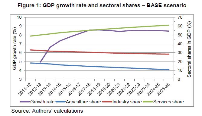 Sectoral prices, however, show the converse trend. Agricultural prices rise sharply compared to both industrial and services prices (Figure 2). In the base year 2011-12, the CPI for all three sectors is nearly same. By 2025-26, however, agricultural products become relatively more expensive – about 2.6 times the price of services and about 1.6 times that of industrial products. The CPI for agricultural products rises by over 60 percentage points over the period 2011-12 to 2025-26. In contrast, the CPI for services fall by about 40 percentage points while CPI of industrial products show a very mild decline during this period. 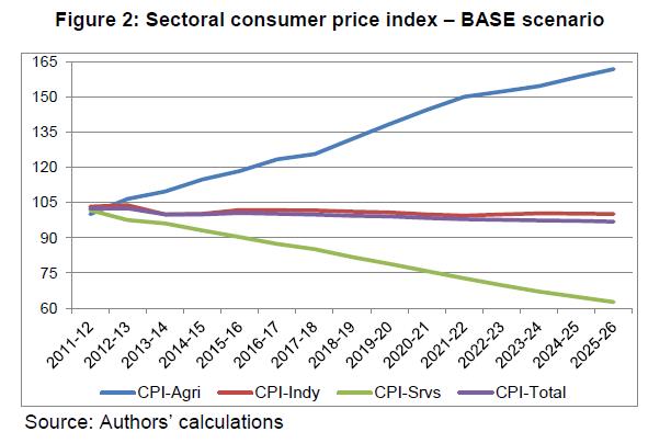 The movements in sectoral price are closely linked to their cost structure, which in turn depends upon their factor use patterns and factor prices. As mentioned earlier, the model distinguishes three types of labour, viz., unskilled, semi-skilled and skilled. While all sectors use all these three labour types, the share of each labour type varies across the sectors, and follows from the usage pattern as captured in the SAM for the base year 2011-12.8 Table 5 shows the total supply of the three types of labour and their usage pattern across sectors. The supply of unskilled labour force is projected to fall over time from about 228 million in 2011-12 to 186 million in 2025-26. In contrast, the supply of both semi-skilled and skilled labour is expected to rise over this period by 75 million and 26 million, respectively, reflecting the progress in education attainment in the country. As a consequence of the change in the supply patterns of the three labour types, the wage structure undergoes a drastic transformation. Real wages of unskilled labour rises dramatically by 3.9 times over the period 2011-12 to 2025-26 (Figure 3) reflecting the shrinking supply of this type of labour. In contrast, the rise in real wages of semi-skilled and skilled labour is quite modest – 1.9 times in the case of semi-skilled labour and just 1.4 times in the case of skilled labour – due to the expansion in their supply which somewhat offsets the positive impact of the overall rise in productivity on their wages. 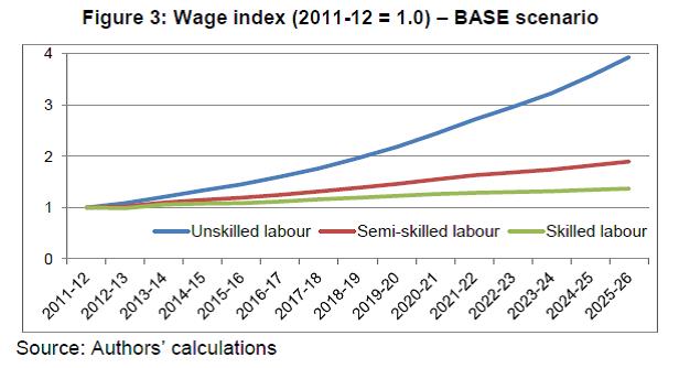
| Table 5: Labour supply and sectoral use pattern (million persons) – BASE scenario | | Year | Unskilled labour | Semi-skilled labour | Skilled labour | | Agri | Ind | Services | Total supply | Agri | Ind | Services | Total supply | Agri | Ind | Services | Total supply | | 2011-12 | 129.6 | 67.3 | 31.5 | 228.3 | 59.1 | 30.8 | 56.2 | 146.1 | 5.1 | 3.5 | 34.4 | 43.0 | | 2012-13 | 131.5 | 66.0 | 29.5 | 227.0 | 63.5 | 32.0 | 55.8 | 151.3 | 5.7 | 3.8 | 35.4 | 44.8 | | 2013-14 | 131.2 | 65.0 | 29.4 | 225.6 | 66.0 | 32.9 | 57.8 | 156.6 | 5.9 | 3.9 | 36.9 | 46.7 | | 2014-15 | 130.8 | 65.0 | 28.0 | 223.8 | 69.3 | 34.6 | 58.0 | 162.0 | 6.4 | 4.2 | 37.9 | 48.5 | | 2015-16 | 129.7 | 65.3 | 26.8 | 221.8 | 72.3 | 36.6 | 58.5 | 167.4 | 6.8 | 4.6 | 39.0 | 50.4 | | 2016-17 | 129.2 | 64.6 | 25.8 | 219.6 | 75.8 | 38.1 | 59.0 | 172.8 | 7.3 | 4.9 | 40.1 | 52.3 | | 2017-18 | 127.1 | 64.8 | 25.1 | 217.0 | 78.1 | 40.0 | 60.2 | 178.3 | 7.6 | 5.1 | 41.4 | 54.2 | | 2018-19 | 126.6 | 63.7 | 23.8 | 214.2 | 82.1 | 41.4 | 60.2 | 183.7 | 8.2 | 5.5 | 42.4 | 56.1 | | 2019-20 | 126.0 | 62.5 | 22.6 | 211.0 | 86.1 | 42.8 | 60.1 | 189.1 | 8.8 | 5.8 | 43.4 | 58.0 | | 2020-21 | 125.1 | 61.3 | 21.2 | 207.6 | 90.4 | 44.4 | 59.7 | 194.5 | 9.5 | 6.1 | 44.2 | 59.9 | | 2021-22 | 123.7 | 60.2 | 19.9 | 203.9 | 94.6 | 46.2 | 59.1 | 199.9 | 10.3 | 6.6 | 44.9 | 61.8 | | 2022-23 | 121.1 | 59.4 | 19.4 | 199.9 | 97.6 | 48.0 | 59.5 | 205.2 | 10.8 | 7.0 | 45.8 | 63.7 | | 2023-24 | 118.3 | 58.4 | 19.0 | 195.7 | 100.6 | 49.8 | 60.0 | 210.5 | 11.4 | 7.4 | 46.7 | 65.5 | | 2024-25 | 115.7 | 57.3 | 18.2 | 191.2 | 104.1 | 51.6 | 60.0 | 215.7 | 12.1 | 7.8 | 47.5 | 67.4 | | 2025-26 | 113.0 | 56.1 | 17.4 | 186.4 | 107.6 | 53.5 | 59.9 | 220.9 | 12.8 | 8.3 | 48.2 | 69.3 | | Source: Authors’ calculations | The use of the three types of labour across sectors is driven by profitability considerations and the production function parameters, which are kept constant in the simulations here. Under this assumption on the technology, it is seen that the use of unskilled (skilled) labour declines (rises) across the board in all sectors. The use of semi-skilled labour rises mainly in agriculture and industry while in services it rises initially up to 2016-17 and stays more or less constant thereafter (Table 5). In terms of deployment across sectors, agriculture’s share in the total demand for unskilled labour actually rises from about 57 per cent in 2011-12 to about 61 per cent in 2025-26, even though the sector’s use of this labour type declines in absolute numbers. In contrast, industry’s share in total demand for unskilled labour remains more or less constant at around 30 per cent while that of services declines from about 14 per cent to 9 per cent. With regard to both semi-skilled and skilled labour, the share of both agriculture and industry in the total demand rises over time while that of services declines commensurately. This demand pattern for the three labour types and the changes in the wage structure seen earlier affects sectoral costs. Agriculture being the largest user of unskilled labour, which witnesses the highest rise in wages, sees a sharp rise in its costs resulting in the sharp rise in its output prices seen earlier (Figure 2). Similarly, industry being another major user of unskilled labour also witnesses a rise in its costs and hence price, though to a much lesser degree than agriculture. In contrast, services sector that uses the least amount of unskilled labour witnesses a decline in its cost and hence its prices relative to the other two sectors. The composition of GDP in terms of various types of expenditure is shown in Figure 4. Private consumption as a percentage of GDP declines rather steadily by about 4 percentage points over the 15-year period. In contrast, government consumption as a percentage of GDP is 2 percentage points higher in the terminal year compared to its initial value. Investments, exports and imports witness some kind of turbulence during the years 2012-13 to 2014-15, when all three of them witness sharp reduction in their shares. Thereafter all three of them witness a steady recovery. By 2025-26, exports is higher by 3 percentage points over its initial value, while investments is only 1 percentage point lower and imports is at the same level as in 2011-12. The current account deficit (CAD) as a percentage of GDP shows much greater movement over this period. In 2011-12 and 2012-13, CAD was about 3.5 per cent and 4.5 per cent of GDP, respectively. Thereafter, it shows a sharp correction to almost 0 per cent in 2014-15. Subsequently, the CAD rises somewhat and fluctuates at around 2 per cent to 2.5 per cent of GDP between 2018-19 and 2025-26. 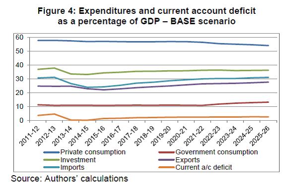 The source of total savings in the economy by institution type is shown in Figure 5. Households account for well over half the total savings in the economy, though their share is projected to come down by about 7.5 percentage points from the 2011-12 level of 65.3 per cent. The share of enterprises (private and public) in total is expected to rise dramatically to about 47 per cent in 2025-26 from 28 per cent in 2011-12. Government is expected to remain a dis-saver and this is expected to worsen over time. Government’s share in total savings deteriorates to -11 per cent in 2025-26 from -3 per cent in 2011-12. Finally, the share of foreign savings shows fluctuations in the initial years, but stabilises later on at around 6 per cent to 7 per cent from 2019-20 onwards. 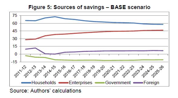 The growth in real income per capita for rural and urban households is shown in Figure 6. In the model, household specific CPI based on their respective consumption pattern is used to compute the real income. Thus, we capture the growth in nominal income and also the changes in relative prices that matter for the each household type. The figure brings out clearly rural-urban divide at each MPCE percentile groups. Indeed, on an absolute basis, the difference is starker for the top 10 per cent MPCE group – the income of the richest rural household is only 30 per cent (33 per cent) of the richest urban household in the year 2011-12 (2025-26). In contrast, the poorest rural household’s income was 75 per cent (102 per cent) of the poorest urban household in the year 2011-12 (2025-26). Over the 15 years, real income per capita doubles for all rural households with the increase being higher for the poorer rural households than for the richer rural households. In contrast, the rise in real income per capita is less than double for all but the richest urban households. In other words, within rural inequality is projected to come down while within urban inequality is expected to rise even as rural-urban inequality is expected to decline, especially for the lower income groups. The distribution of savings across various household classes is shown in Table 6. In 2011-12, 84 per cent of household savings were accounted for by the top 30 per cent of households in rural and urban areas, with about 37 per cent coming from the rural top 30 per cent and the balance 47 per cent from the urban top 30 per cent. Over time, with real incomes growing across all households, the share of the top 30 per cent of the households is projected to come down by 7 percentage points to about 77 per cent in the terminal year. Interestingly, the gap in the shares of rural and urban top 30 per cent of households is projected to narrow down over time 38 per cent for the rural top 30 per cent versus 39 per cent for their urban counterparts. Another interesting aspect of these projections is that in the terminal year the bottom 70 per cent of rural population is projected to account for 15 per cent of total household savings while their urban counterparts are expected to contribute only 8 per cent. 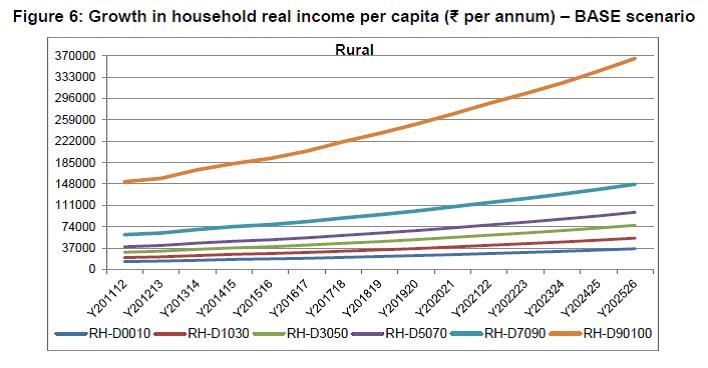
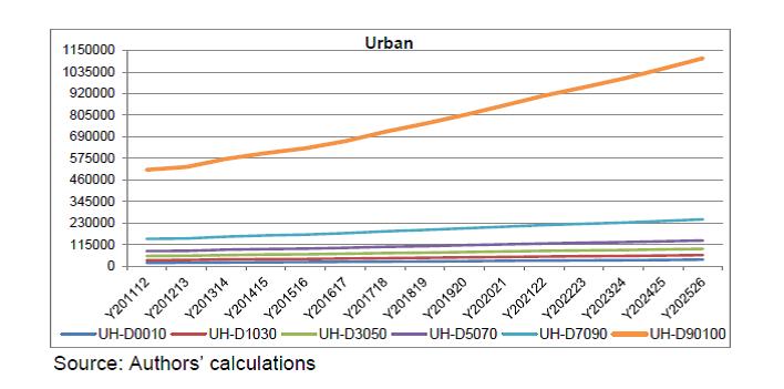
| Table 6: Share of households in total household savings (per cent) – BASE scenario | | | 2011-12 | 2012-13 | 2013-14 | 2014-15 | 2015-16 | 2016-17 | 2017-18 | 2018-19 | 2019-20 | 2020-21 | 2021-22 | 2022-23 | 2023-24 | 2024-25 | 2025-26 | | RH-D0010 | -0.1 | 0.0 | 0.0 | 0.1 | 0.2 | 0.2 | 0.3 | 0.3 | 0.3 | 0.4 | 0.4 | 0.5 | 0.5 | 0.5 | 0.5 | | RH-D1030 | 0.6 | 0.8 | 1.0 | 1.2 | 1.3 | 1.4 | 1.5 | 1.6 | 1.7 | 1.9 | 2.0 | 2.0 | 2.1 | 2.2 | 2.3 | | RH-D3050 | 3.3 | 3.6 | 3.6 | 3.8 | 3.9 | 4.0 | 4.1 | 4.2 | 4.3 | 4.4 | 4.5 | 4.5 | 4.6 | 4.6 | 4.7 | | RH-D5070 | 5.1 | 5.5 | 5.7 | 6.0 | 6.1 | 6.3 | 6.4 | 6.6 | 6.8 | 6.9 | 7.1 | 7.2 | 7.3 | 7.4 | 7.5 | | RH-D7090 | 12.0 | 12.4 | 12.6 | 12.9 | 13.0 | 13.2 | 13.4 | 13.6 | 13.8 | 14.0 | 14.1 | 14.2 | 14.4 | 14.5 | 14.6 | | RH-D90100 | 24.6 | 24.4 | 24.3 | 24.0 | 23.9 | 23.8 | 23.7 | 23.6 | 23.5 | 23.4 | 23.3 | 23.2 | 23.2 | 23.1 | 23.0 | | UH-D0010 | -0.4 | -0.4 | -0.3 | -0.3 | -0.2 | -0.2 | -0.1 | -0.1 | -0.1 | 0.0 | 0.0 | 0.0 | 0.1 | 0.1 | 0.1 | | UH-D1030 | 0.3 | 0.4 | 0.5 | 0.6 | 0.6 | 0.7 | 0.7 | 0.8 | 0.8 | 0.9 | 0.9 | 1.0 | 1.0 | 1.0 | 1.1 | | UH-D3050 | 2.7 | 2.7 | 2.7 | 2.7 | 2.7 | 2.7 | 2.7 | 2.7 | 2.6 | 2.6 | 2.6 | 2.6 | 2.6 | 2.6 | 2.6 | | UH-D5070 | 4.7 | 4.7 | 4.6 | 4.7 | 4.6 | 4.6 | 4.6 | 4.6 | 4.6 | 4.6 | 4.6 | 4.6 | 4.5 | 4.5 | 4.5 | | UH-D7090 | 11.9 | 11.7 | 11.6 | 11.4 | 11.3 | 11.1 | 11.1 | 10.9 | 10.8 | 10.7 | 10.5 | 10.4 | 10.3 | 10.2 | 10.1 | | UH-D90100 | 35.2 | 34.2 | 33.8 | 32.9 | 32.7 | 32.2 | 31.8 | 31.3 | 30.8 | 30.3 | 29.9 | 29.7 | 29.4 | 29.2 | 28.9 | | Share of households in total savings | 65.3 | 64.9 | 70.4 | 72.7 | 68.8 | 67.3 | 64.9 | 63.3 | 62.4 | 61.5 | 61.1 | 60.4 | 58.8 | 58.0 | 57.8 | | Source: Authors’ calculation | As described earlier, the model projects commodity-wise demand through household-wise linear expenditure demand system. Figure 7 shows the shares of agricultural, industrial and services products in total consumption aggregated over all households. As may be expected the share of agricultural products is projected to decline steadily over time from about 25 per cent in 2011-12 to just 11 per cent in 2025-26. In contrast the share of industrial products is projected to rise from 35 per cent to 50 per cent over this period. The share of services show a slight rise from 40 per cent in 2011-12 to 42 per cent in 2018-19 and then declines to about 39 per cent in the terminal year. 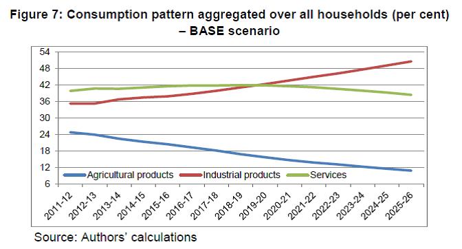 The distribution of demand across household classes is shown in Table 7. In the case of agricultural products in 2011-12 two-thirds of the demand came from rural households. Over time, however, the share of urban households is projected to rise by 5 percentage points from about 33 per cent to 38 per cent, and correspondingly the share of rural households is expected to decline. The reverse is projected to happen in the case of demand for industrial products. In this case, the share of rural households is projected to rise from about 59 per cent in 2011-12 to 64 per cent in 2025-26, and accordingly the share of urban households is expected to fall. With regard to demand for services, the pattern is similar to that of agricultural products. Rural households’ share is expected to decline slightly from 41 per cent to 37 per cent, while urban households’ share is expected to rise commensurately over the projection period. Thus far, we have described the model projections in the BASE scenario for certain critical variables of interest. In the following sections we discuss the results for each set of policy simulations. The model outcomes for various variables of interest are compared with their corresponding values in the BASE scenario. The difference in the values for a particular simulation with the BASE scenario can then be ascribed to the policy shock/ closure specified in that simulation. | Table 7: Distribution of consumption across household classes (per cent) – BASE scenario | | | 2011-12 | 2012-13 | 2013-14 | 2014-15 | 2015-16 | 2016-17 | 2017-18 | 2018-19 | 2019-20 | 2020-21 | 2021-22 | 2022-23 | 2023-24 | 2024-25 | 2025-26 | | Agricultural products | | | | | | | | | | | | | | | | | Rural - bottom 70% | 37.6 | 37.7 | 37.5 | 37.5 | 37.3 | 37.0 | 36.8 | 36.6 | 36.4 | 36.2 | 36.0 | 35.8 | 35.5 | 35.2 | 35.0 | | Rural - bottom 90% | 54.7 | 54.7 | 54.4 | 54.3 | 54.0 | 53.6 | 53.2 | 53.0 | 52.6 | 52.3 | 52.0 | 51.6 | 51.2 | 50.8 | 50.5 | | Rural - all | 67.1 | 67.1 | 66.8 | 66.5 | 66.2 | 65.8 | 65.3 | 65.0 | 64.6 | 64.2 | 63.7 | 63.2 | 62.8 | 62.3 | 61.8 | | Urban - bottom 70% | 18.5 | 18.6 | 18.7 | 18.9 | 19.1 | 19.3 | 19.5 | 19.7 | 19.9 | 20.2 | 20.4 | 20.7 | 21.0 | 21.2 | 21.5 | | Urban - bottom 90% | 27.0 | 27.1 | 27.3 | 27.5 | 27.8 | 28.1 | 28.4 | 28.7 | 29.0 | 29.3 | 29.7 | 30.1 | 30.5 | 30.9 | 31.3 | | Urban - all | 32.9 | 32.9 | 33.2 | 33.5 | 33.8 | 34.2 | 34.7 | 35.0 | 35.4 | 35.8 | 36.3 | 36.8 | 37.2 | 37.7 | 38.2 | | Industrial products | | | | | | | | | | | | | | | | | Rural - bottom 70% | 30.5 | 31.2 | 31.3 | 31.9 | 32.2 | 32.4 | 32.3 | 32.5 | 32.6 | 32.8 | 33.1 | 33.4 | 33.4 | 33.5 | 33.7 | | Rural - bottom 90% | 45.2 | 45.9 | 46.0 | 46.7 | 47.1 | 47.3 | 47.3 | 47.5 | 47.7 | 48.0 | 48.4 | 48.7 | 48.8 | 49.0 | 49.2 | | Rural - all | 58.9 | 59.5 | 59.8 | 60.4 | 60.9 | 61.3 | 61.5 | 62.0 | 62.3 | 62.7 | 63.1 | 63.5 | 63.7 | 63.9 | 64.1 | | Urban - bottom 70% | 19.2 | 19.0 | 18.5 | 18.3 | 17.9 | 17.5 | 17.1 | 16.7 | 16.3 | 16.0 | 15.7 | 15.4 | 15.1 | 14.9 | 14.7 | | Urban - bottom 90% | 29.7 | 29.3 | 28.7 | 28.2 | 27.6 | 27.0 | 26.5 | 25.8 | 25.3 | 24.8 | 24.3 | 23.9 | 23.4 | 23.0 | 22.7 | | Urban - all | 41.1 | 40.5 | 40.2 | 39.6 | 39.1 | 38.7 | 38.5 | 38.0 | 37.7 | 37.3 | 36.9 | 36.5 | 36.3 | 36.1 | 35.9 | | Services | | | | | | | | | | | | | | | | | Rural - bottom 70% | 16.3 | 16.6 | 16.5 | 16.7 | 16.7 | 16.5 | 16.3 | 16.1 | 16.0 | 15.9 | 15.8 | 15.7 | 15.5 | 15.3 | 15.1 | | Rural - bottom 90% | 27.3 | 27.7 | 27.5 | 27.7 | 27.6 | 27.4 | 27.0 | 26.8 | 26.5 | 26.3 | 26.2 | 26.0 | 25.6 | 25.3 | 25.0 | | Rural - all | 40.5 | 40.8 | 40.7 | 40.8 | 40.8 | 40.5 | 40.1 | 39.9 | 39.6 | 39.3 | 38.9 | 38.5 | 38.1 | 37.6 | 37.1 | | Urban - bottom 70% | 19.4 | 19.3 | 19.0 | 19.0 | 18.8 | 18.6 | 18.3 | 18.1 | 18.0 | 17.9 | 17.9 | 18.0 | 17.9 | 17.9 | 18.0 | | Urban - bottom 90% | 35.7 | 35.4 | 34.9 | 34.7 | 34.4 | 34.1 | 33.8 | 33.4 | 33.2 | 33.1 | 33.0 | 33.1 | 33.0 | 33.0 | 33.1 | | Urban - all | 59.5 | 59.2 | 59.3 | 59.2 | 59.2 | 59.5 | 59.9 | 60.1 | 60.4 | 60.7 | 61.1 | 61.5 | 61.9 | 62.4 | 62.9 | | Source: Authors’ calculations | 4.2 Set-A: Impact of a rise in government consumption expenditure To recall, in all the 4 simulations that we carry out in Set-A, we increase government consumption expenditure by 10 per cent each year starting from 2016-17 over the corresponding level in the BASE scenario.9 These 4 simulations vary only in their macroeconomic closure. In RUN-01 and RUN-03 we specify full employment of all factors of production while in RUN-02 and RUN-04 we allow for unemployment. Besides this, in RUN-01 and RUN-02 we fix the exchange rate at the BASE level and allow foreign capital flows to adjust, while in RUN-03 and RUN-04 we specify the converse. In all 4 simulations, the model is savings driven. The results show that despite keeping the magnitude of fiscal expansion constant across the 4 simulations government consumption as a percentage of GDP varies across them (Figure 8). The implied GDP multipliers of public expenditure for all the scenarios are presented in Appendix 3, Appendix Table 1. It is seen that government consumption as a percentage of GDP is lowest in the BASE, followed by RUN-02 and RUN-04 with nearly the same levels, then RUN-03 and is highest in RUN-01. The implied multipliers for RUN-02 and RUN-04 are about 0.6 to 0.7, while they are negative for RUN-01 and RUN-03. The reason for this is that GDP growth differs across them, which can be attributed to the differences in the macroeconomic closure specification. 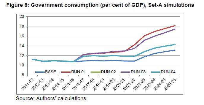 The impact of the rise in government consumption on the level of GDP across the 4 simulations is presented in Figure 9, and the annual rate of growth in GDP is presented in Figure 10. These results show some clear and interesting patterns. In RUN-02 and RUN-04 where there are unemployed factors, a short-term boost to both the level and growth rate of GDP is seen in 2016-17, the first year when fiscal expansion takes place. Compared to the BASE scenario the level of GDP is higher in these two simulations by about 0.8 per cent in 2016-17 and this difference rises gradually to about 1 per cent in the terminal year. The growth rate of GDP also rises to about 9.1 per cent in 2016-17, but thereafter settles back to the level in BASE scenario. In both these scenarios, employment of all three types of labour expands at varying rates. Employment of unskilled and semi-skilled labour expands by about 0.2 per cent over the BASE levels (Figure 11) while that of semi-skilled labour rises somewhat more at about 0.5 per cent. Skilled labour employment rises much more drastically around 1.8 per cent to 2 per cent over the years across these two scenarios. The differential impact on employment of the three labour types is consistent with the trends in their size and employment pattern in the BASE scenario. In contrast, in RUN-01 and RUN-03 where there is full employment of all factors, the level of GDP declines immediately after the fiscal expansion compared to BASE levels. Over time both the level and the growth rate of GDP falls quite dramatically in both these scenarios. In RUN-01 (RUN-03), the level of GDP in the terminal year is 3.8 per cent (7.9 per cent) lower than in BASE, and the growth rate in the terminal year is just 7.7 per cent (6.3 per cent) compared to about 8.5 per cent in BASE, RUN-02 and RUN-04. Therein is an important message, viz., that the timing of fiscal expansion is critical. Fiscal expansion would be disastrous when undertaken during boom phases when factors of production are already fully employed, but can be helpful when there are unemployed resources as during recessions. The main reason behind this differential impact of fiscal expansion on GDP growth is its effect on government’s (dis-)saving and hence the total savings and investment in the economy. In RUN-02 and RUN-04, government dis-saving is about 21 per cent to 23 per cent higher than in BASE (Figure 12). In contrast, in RUN-01 and RUN-03 especially, government dis-saving is much higher than in BASE and it increases over time. In RUN-03, it is about 158 per cent higher than BASE in the terminal year, whereas it is about 47 per cent higher in RUN-01. As a result in RUN-01 and RUN-03 total savings and investment are much lower than in BASE (Figure 13). In both these simulations, the shortfall in investments compared to BASE increases over time. In RUN-01, it increases from about -3.5 per cent in 2016-17 to about -10.5 per cent in 2025-26, while in RUN-03 it goes up from -4.5 per cent to about -41.5 per cent over this period. In contrast, in RUN-02 and RUN-04, investment levels are lower than BASE but by only about 2 per cent all through. As a percentage of GDP also investment in RUN-02, RUN-04 and RUN-01 are somewhat lower than in BASE, though it rises over time in all these 3 simulations (Figure 14). In contrast in RUN-03 investment as a percentage of GDP declines over time, reflecting the sharp decline in savings in this simulation. The above results also highlight the usefulness of the recursive CGE model used in this study. An expansion of government consumption expenditure under full employment that triggers a change in the sectoral composition of demand can be expected to affect GDP in the short-run. Indeed, all static CGE models would capture this effect routinely. However, static models will not be able to capture the long-run impact of such expenditure switching that affects capital formation and hence the future potential/ full employment level output. Only a model that captures inter-temporal dynamics, such as the recursive CGE model used here, can bring out these long-run impacts. The slowdown in GDP growth across these simulations also results in a corresponding slowdown in both exports and imports (Figures 15 and 16). The slowdown in exports is highest in RUN-01 and RUN-03 where GDP growth is the slowest. As a percentage of GDP exports in the terminal year in these two simulations is barely 25 per cent, about 3 percentage points less than in BASE. Not surprisingly, the current account deficit shoots up in RUN-01 and RUN-03 much more than in the other simulations (Figure 17). In the terminal year it is about 3.8 per cent in RUN-03 and 4.2 per cent in RUN-01, reflecting the slowdown in GDP and additionally the depreciation of the Rupee in RUN-03. These simulations also bring out another important message pertaining to the role of foreign capital flows. Considering the growth outcomes of RUN-01 and RUN-03 as a pair and RUN-02 and RUN-04 as another pair we see that tightness in foreign capital flow in the presence of unemployed factors matters less for growth but can be very critical when there is full employment in the economy. When fiscal expansion happens under conditions of full employment, and if additional foreign capital flow to sustain this expansion is not forthcoming as in RUN-03, the ensuing resource crunch causes the exchange rate to depreciate significantly. This can be seen in Figure 18. In contrast, when there are unemployed resources available the output growth that follows fiscal expansion makes available additional tax revenues for the government to finance its enhanced expenditure, and thereby it does not cause a resource crunch. Consequently, even if foreign capital inflows are not forthcoming, as in RUN-04, the exchange rate does not depreciate. 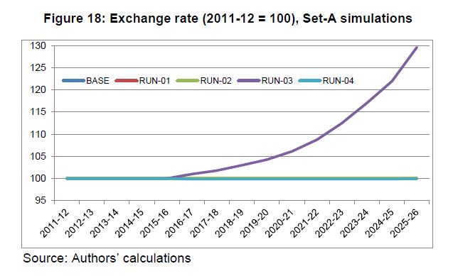 It must be noted here that in the CGE model macro indicators such as the GDP, savings, aggregate exports and imports, and the CAD, are obtained by aggregating the corresponding micro-level flows (such as sectoral value added, sectoral exports and imports, agent-wise savings, etc.). Although the simulations in this set show significant change at a macro level in some of the simulations, at the sectoral level, the impacts in terms of shares in GDP and relative prices do not show much variation across these simulations compared to the BASE. As in the BASE, agriculture’s share falls over time across all these simulations, while that of services rises significantly, and industry’s share shows a very slight fall over time. With regard to prices too, the CPI for these three broad sectors in these simulations show a similar pattern across these simulations as in the BASE. These sectoral movements are reported in Appendix 3 (Appendix Figure 3). At the household level, however, some significant impacts are seen in these simulations. The level and growth in real income per capita across all households put together are shown in Figures 19 and 20, respectively. Significant reduction in the level and growth rate as compared to the BASE scenario is seen in the case of RUN-01 and RUN-03, especially the latter. These two simulations are also the ones that witnessed significant reduction in the GDP growth rate. In contrast, in RUN-02 and RUN-04 the level real income per capita is slightly higher than BASE and its growth rate is almost the same as in the BASE, again reflecting the GDP growth in these two simulations. A similar pattern is seen across these simulations in the level and growth in real income per capita observed at the level of individual household classes also.10 However, no systematic change in the inequality across households is seen across these simulations.   4.3 Set-B: Nature of relationship between government expenditure and GDP The second question that we are concerned with is the nature of the relationship between government expenditure and GDP. Does the impact on GDP depend upon the quantum of rise in government expenditure? If it does then it would imply a nonlinear relationship; linear otherwise. We address this question in this set through the 4 simulations, viz., RUN-05 to RUN-08, all of which have the same specification as RUN-04 of Set-A above including the macroeconomic closure except for the magnitude of rise in government expenditure. As mentioned earlier, in RUN-05, the quantum of fiscal expansion is 5 per cent over BASE level, while in RUN-06, RUN-07 and RUN-08 it is 15 per cent, 20 per cent and 25 per cent, respectively. Along with RUN-04 where the quantum of fiscal expansion is 10 per cent over BASE level, these 4 simulations would help us understand if the relationship between government expenditure and GDP is linear or non-linear. The simulation results suggest that the relationship between government expenditure and GDP is fairly linear. In the first year after the shock is introduced, the level of GDP rises by roughly 0.4 per cent to 0.5 per cent over the BASE level for every 5 percentage point increase in government expenditure across these simulations including RUN-04 (Figure 21). In the subsequent years too, the difference in the GDP level across these simulations is more or less of a similar order. That is, there is only a (near) constant level difference in the GDP across these simulations suggesting a fairly linear relationship. This is also seen in terms of the GDP growth rates in Figure 22, which shows that it is only in the first year that the growth rate varies across the simulations reflecting the level jump in GDP seen earlier. Thereafter, the growth rate is virtually the same across these simulations reflecting the more or less parallel trajectory over time seen in Figure 21.11 Household real income per capita also shows a similar linear relationship with government consumption expenditure though the magnitude of change is slightly lower than that of aggregate GDP (Figure 23). Compared with BASE, every 5 percentage point rise in government expenditure adds about 0.2 per cent to 0.3 per cent to household real income per capita. Not surprisingly, the additional employment generated also shows a similar linear relationship across these scenarios (Table 8). Indeed, such a linear relationship is seen in several other macroeconomic variables of interest such as government dis-savings, investment, sectoral shares in GDP, trade flows, real income per capita, private consumption, etc. (Table 9). It must be noted here that we arrive at this conclusion based on a detailed CGE model in which most of the equations that characterise production, consumption, trade, income distribution across factors and agents of the economy, and various government policies, are all non-linear. Further, it is worth stressing that GDP in our model is computed by aggregating sectoral value added, which is endogenously determined based on demand and supply conditions faced by individual sectors as well as in the factor markets, which affect both product and factor prices and hence returns to factors, all of which are endogenous in the model.
| Table 8: Rise in labour employment (per cent change over BASE scenario), Set-B simulations | | Scenario | 2016-17 | 2017-18 | 2018-19 | 2019-20 | 2020-21 | 2021-22 | 2022-23 | 2023-24 | 2024-25 | 2025-26 | | | Unskilled labour | | RUN-04 | 0.12 | 0.09 | 0.08 | 0.07 | 0.07 | 0.07 | 0.08 | 0.10 | 0.11 | 0.11 | | RUN-05 | 0.06 | 0.05 | 0.04 | 0.04 | 0.04 | 0.04 | 0.04 | 0.05 | 0.05 | 0.06 | | RUN-06 | 0.17 | 0.14 | 0.12 | 0.11 | 0.10 | 0.10 | 0.13 | 0.15 | 0.16 | 0.17 | | RUN-07 | 0.23 | 0.18 | 0.16 | 0.14 | 0.14 | 0.14 | 0.17 | 0.19 | 0.21 | 0.22 | | RUN-08 | 0.28 | 0.22 | 0.19 | 0.18 | 0.17 | 0.17 | 0.20 | 0.24 | 0.26 | 0.28 | | | Semi-skilled labour | | RUN-04 | 0.55 | 0.53 | 0.50 | 0.49 | 0.47 | 0.45 | 0.47 | 0.47 | 0.47 | 0.47 | | RUN-05 | 0.28 | 0.26 | 0.25 | 0.25 | 0.24 | 0.23 | 0.24 | 0.24 | 0.24 | 0.24 | | RUN-06 | 0.82 | 0.79 | 0.75 | 0.73 | 0.70 | 0.68 | 0.70 | 0.71 | 0.71 | 0.70 | | RUN-07 | 1.09 | 1.05 | 1.00 | 0.97 | 0.93 | 0.90 | 0.93 | 0.94 | 0.94 | 0.93 | | RUN-08 | 1.36 | 1.31 | 1.24 | 1.21 | 1.16 | 1.12 | 1.16 | 1.17 | 1.17 | 1.16 | | | Skilled labour | | RUN-04 | 1.88 | 1.87 | 1.83 | 1.83 | 1.80 | 1.77 | 1.81 | 1.80 | 1.80 | 1.79 | | RUN-05 | 0.94 | 0.94 | 0.92 | 0.92 | 0.90 | 0.89 | 0.91 | 0.90 | 0.90 | 0.90 | | RUN-06 | 2.82 | 2.80 | 2.74 | 2.74 | 2.69 | 2.66 | 2.71 | 2.69 | 2.70 | 2.68 | | RUN-07 | 3.75 | 3.73 | 3.65 | 3.65 | 3.59 | 3.54 | 3.61 | 3.58 | 3.59 | 3.57 | | RUN-08 | 4.68 | 4.66 | 4.56 | 4.55 | 4.47 | 4.41 | 4.50 | 4.47 | 4.48 | 4.45 | | Source: Authors’ calculations |
| Table 9: Set-B simulation results (percentage change from RUN-04) | | Variable (unit of measurement) | 2016-17 | 2017-18 | 2018-19 | 2019-20 | 2020-21 | 2021-22 | 2022-23 | 2023-24 | 2024-25 | 2025-26 | 2016-17 | 2017-18 | 2018-19 | 2019-20 | 2020-21 | 2021-22 | 2022-23 | 2023-24 | 2024-25 | 2025-26 | | | RUN-05 | RUN-06 | | Government consumption (as % of GDP) | -4.1 | -4.1 | -4.1 | -4.1 | -4.1 | -4.1 | -4.1 | -4.1 | -4.0 | -4.0 | 4.1 | 4.1 | 4.1 | 4.1 | 4.1 | 4.1 | 4.0 | 4.0 | 4.0 | 4.0 | | Government dis-savings (₹ '000 Crores) | -9.0 | -9.1 | -9.1 | -8.7 | -8.7 | -8.7 | -8.9 | -9.4 | -9.4 | -9.4 | 9.0 | 9.1 | 9.1 | 8.7 | 8.7 | 8.7 | 8.8 | 9.4 | 9.3 | 9.4 | | Gross fixed capital formation (₹ '000 Crores) | 1.0 | 1.0 | 1.1 | 1.1 | 1.1 | 1.1 | 1.1 | 1.1 | 1.1 | 1.1 | -1.0 | -1.0 | -1.0 | -1.1 | -1.1 | -1.1 | -1.1 | -1.1 | -1.1 | -1.1 | | Investment (as % of GDP) | 1.3 | 1.3 | 1.3 | 1.3 | 1.3 | 1.3 | 1.4 | 1.4 | 1.4 | 1.4 | -1.3 | -1.3 | -1.3 | -1.3 | -1.3 | -1.3 | -1.3 | -1.4 | -1.4 | -1.4 | | GDP-Agriculture (as % of GDP) | 0.4 | 0.4 | 0.4 | 0.4 | 0.4 | 0.5 | 0.5 | 0.5 | 0.5 | 0.5 | -0.4 | -0.4 | -0.4 | -0.4 | -0.4 | -0.4 | -0.5 | -0.5 | -0.5 | -0.5 | | GDP-Industry (as % of GDP) | 0.5 | 0.5 | 0.5 | 0.6 | 0.6 | 0.6 | 0.6 | 0.6 | 0.6 | 0.6 | -0.5 | -0.5 | -0.5 | -0.5 | -0.5 | -0.5 | -0.6 | -0.6 | -0.6 | -0.6 | | GDP-Services (as % of GDP) | -0.4 | -0.4 | -0.4 | -0.4 | -0.4 | -0.4 | -0.4 | -0.4 | -0.4 | -0.4 | 0.4 | 0.4 | 0.4 | 0.4 | 0.4 | 0.4 | 0.4 | 0.4 | 0.4 | 0.3 | | Exports (as % of GDP) | 0.2 | 0.2 | 0.2 | 0.2 | 0.2 | 0.2 | 0.3 | 0.3 | 0.3 | 0.3 | -0.2 | -0.2 | -0.2 | -0.2 | -0.2 | -0.2 | -0.3 | -0.3 | -0.3 | -0.3 | | Imports (as % of GDP) | 0.3 | 0.3 | 0.2 | 0.2 | 0.2 | 0.2 | 0.3 | 0.3 | 0.3 | 0.3 | -0.3 | -0.2 | -0.2 | -0.2 | -0.2 | -0.2 | -0.3 | -0.3 | -0.3 | -0.3 | | Current account (as % of GDP) | 0.4 | 0.4 | 0.4 | 0.4 | 0.3 | 0.3 | 0.4 | 0.4 | 0.4 | 0.4 | -0.4 | -0.4 | -0.4 | -0.4 | -0.3 | -0.3 | -0.4 | -0.4 | -0.4 | -0.4 | | Exchange rate (2011-12 = 100) | 0.1 | 0.1 | 0.1 | 0.1 | 0.1 | 0.1 | 0.1 | 0.1 | 0.0 | 0.0 | -0.1 | -0.1 | -0.1 | -0.1 | -0.1 | -0.1 | -0.1 | -0.1 | -0.1 | 0.0 | | Real income per capita, rural households (₹) | -0.2 | -0.2 | -0.2 | -0.2 | -0.2 | -0.2 | -0.2 | -0.2 | -0.2 | -0.2 | 0.2 | 0.2 | 0.2 | 0.2 | 0.2 | 0.2 | 0.2 | 0.2 | 0.2 | 0.2 | | Real income per capita, urban households (₹) | -0.4 | -0.4 | -0.4 | -0.4 | -0.4 | -0.4 | -0.4 | -0.4 | -0.4 | -0.4 | 0.4 | 0.4 | 0.4 | 0.4 | 0.4 | 0.4 | 0.4 | 0.4 | 0.4 | 0.4 | | Real income per capita, all households (₹) | -0.3 | -0.3 | -0.3 | -0.3 | -0.3 | -0.3 | -0.3 | -0.3 | -0.3 | -0.3 | 0.3 | 0.3 | 0.3 | 0.3 | 0.3 | 0.3 | 0.3 | 0.3 | 0.3 | 0.3 | | Private consumption (as % of GDP) | 0.1 | 0.1 | 0.1 | 0.1 | 0.1 | 0.1 | 0.1 | 0.1 | 0.1 | 0.2 | -0.1 | -0.1 | -0.1 | -0.1 | -0.1 | -0.1 | -0.1 | -0.1 | -0.1 | -0.2 | | | RUN-07 | RUN-08 | | Government consumption (as % of GDP) | 8.1 | 8.1 | 8.1 | 8.1 | 8.1 | 8.1 | 8.0 | 8.0 | 8.0 | 7.9 | 12.1 | 12.1 | 12.1 | 12.1 | 12.1 | 12.1 | 12.0 | 11.9 | 11.9 | 11.9 | | Government dis-savings (₹ '000 Crores) | 18.0 | 18.1 | 18.1 | 17.4 | 17.3 | 17.3 | 17.7 | 18.8 | 18.6 | 18.7 | 26.9 | 27.1 | 27.1 | 26.0 | 25.9 | 25.9 | 26.5 | 28.1 | 27.9 | 28.0 | | Gross fixed capital formation (₹ '000 Crores) | -2.0 | -2.1 | -2.1 | -2.2 | -2.2 | -2.1 | -2.2 | -2.2 | -2.2 | -2.2 | -3.0 | -3.1 | -3.1 | -3.2 | -3.2 | -3.2 | -3.3 | -3.3 | -3.3 | -3.3 | | Investment (as % of GDP) | -2.5 | -2.5 | -2.5 | -2.6 | -2.6 | -2.6 | -2.7 | -2.8 | -2.8 | -2.8 | -3.7 | -3.8 | -3.8 | -3.9 | -3.9 | -3.8 | -4.0 | -4.1 | -4.2 | -4.2 | | GDP-Agriculture (as % of GDP) | -0.8 | -0.8 | -0.8 | -0.9 | -0.9 | -0.9 | -0.9 | -0.9 | -1.0 | -1.0 | -1.1 | -1.2 | -1.2 | -1.3 | -1.3 | -1.3 | -1.4 | -1.4 | -1.4 | -1.4 | | GDP-Industry (as % of GDP) | -1.1 | -1.1 | -1.1 | -1.1 | -1.1 | -1.1 | -1.1 | -1.1 | -1.1 | -1.1 | -1.6 | -1.6 | -1.6 | -1.6 | -1.6 | -1.6 | -1.7 | -1.7 | -1.7 | -1.7 | | GDP-Services (as % of GDP) | 0.8 | 0.8 | 0.8 | 0.8 | 0.7 | 0.7 | 0.7 | 0.7 | 0.7 | 0.7 | 1.2 | 1.2 | 1.1 | 1.1 | 1.1 | 1.1 | 1.1 | 1.1 | 1.0 | 1.0 | | Exports (as % of GDP) | -0.5 | -0.5 | -0.4 | -0.4 | -0.4 | -0.4 | -0.5 | -0.6 | -0.6 | -0.6 | -0.7 | -0.7 | -0.7 | -0.7 | -0.6 | -0.6 | -0.8 | -0.9 | -0.9 | -1.0 | | Imports (as % of GDP) | -0.5 | -0.5 | -0.5 | -0.5 | -0.5 | -0.5 | -0.5 | -0.6 | -0.6 | -0.7 | -0.7 | -0.7 | -0.7 | -0.7 | -0.7 | -0.7 | -0.8 | -0.9 | -0.9 | -1.0 | | Current account (as % of GDP) | -0.8 | -0.7 | -0.7 | -0.7 | -0.7 | -0.7 | -0.7 | -0.8 | -0.8 | -0.8 | -1.1 | -1.1 | -1.1 | -1.1 | -1.0 | -1.0 | -1.1 | -1.2 | -1.2 | -1.3 | | Exchange rate (2011-12 = 100) | -0.1 | -0.1 | -0.1 | -0.1 | -0.1 | -0.1 | -0.1 | -0.1 | -0.1 | -0.1 | -0.2 | -0.2 | -0.2 | -0.2 | -0.2 | -0.2 | -0.2 | -0.2 | -0.2 | -0.1 | | Real income per capita, rural households (₹) | 0.5 | 0.5 | 0.4 | 0.4 | 0.4 | 0.4 | 0.4 | 0.4 | 0.4 | 0.4 | 0.7 | 0.7 | 0.7 | 0.7 | 0.6 | 0.6 | 0.6 | 0.6 | 0.6 | 0.6 | | Real income per capita, urban households (₹) | 0.8 | 0.8 | 0.8 | 0.8 | 0.8 | 0.8 | 0.8 | 0.8 | 0.8 | 0.8 | 1.2 | 1.2 | 1.2 | 1.2 | 1.2 | 1.2 | 1.3 | 1.2 | 1.2 | 1.2 | | Real income per capita, all households (₹) | 0.6 | 0.6 | 0.6 | 0.6 | 0.6 | 0.6 | 0.6 | 0.6 | 0.6 | 0.6 | 0.9 | 0.9 | 0.9 | 0.9 | 0.9 | 0.9 | 1.0 | 0.9 | 0.9 | 0.9 | | Private consumption (as % of GDP) | -0.2 | -0.2 | -0.2 | -0.2 | -0.1 | -0.1 | -0.2 | -0.3 | -0.3 | -0.3 | -0.3 | -0.3 | -0.3 | -0.2 | -0.2 | -0.2 | -0.3 | -0.4 | -0.4 | -0.5 | | Source: Authors’ calculations | 4.4 Set-C: Impact of a rise in government expenditure in specific sectors As described earlier, we carry out 2 simulations in Set-C wherein government expenditure is increased in specific sectors, in particular the social sectors (water supply, education and medical services) in RUN-09 and on public administration (part of Services-2 sector) in RUN-10. In both these simulations, we maintain the same quantum of rise in government expenditure as well as the macroeconomic closure as in simulations RUN-04 of Set-A. That is, we allow for unemployment and keep the foreign capital flow fixed at the BASE levels. The simulations show that focusing additional government expenditure on particular sectors results in a rise in the GDP level by about 1 per cent in 2016-17 compared to BASE level, which amounts to a rise of just 20 basis points over and above what was seen in RUN-04 (Figure 24). Indeed in the later years too, GDP level in both RUN-09 and RUN-10 is somewhat more than in RUN-04, though the difference is not very large. Consequently, in terms of GDP growth rates focusing additional government expenditure on particular sectors does not have any significant extra impact compared to the case when the additional expenditure is broad-based.  In terms of employment generation, however, the two scenarios show some differences. Employment generation in RUN-09 is somewhat less than in RUN-04 while opposite is the case in RUN-10 (Table 10). Thus, from a purely employment perspective, our results suggest that public expenditure on administrative services appears to have a higher employment multiplier than expenditure on social sectors or even general fiscal expansion, even though there are no tangible effects on GDP growth rates, as mentioned earlier. The results also show that it is not just GDP growth rate that does not show any difference in the Set-C simulations compared to RUN-04. Several other variables such as gross fixed capital formation, various expenditure categories as a percentage of GDP, sectoral shares in aggregate GDP, sectoral relative prices, as well as real income per capita of households show only a small difference (less than half a percent deviation) in the two Set-C simulations over their corresponding level in RUN-04 (Table 10). It is only the level of government dis-savings that shows a somewhat large difference compared to its level in RUN-04. But this hardly has any impact on aggregate GDP as seen earlier due to the small adjustments that are spread out across several variables in the economy. | Table 10: Set-C simulation results (percentage change from RUN-04) | | Variable (unit of measurement) | 2016-17 | 2017-18 | 2018-19 | 2019-20 | 2020-21 | 2021-22 | 2022-23 | 2023-24 | 2024-25 | 2025-26 | | | RUN-09 | | Additional employment - Unskilled labour | -0.2 | -0.2 | -0.1 | -0.2 | -0.1 | -0.1 | -0.1 | 0.0 | 0.0 | 0.0 | | Additional employment - Semi-skilled labour | -0.4 | -0.3 | -0.3 | -0.3 | -0.3 | -0.3 | -0.3 | -0.2 | -0.2 | -0.2 | | Additional employment - Skilled labour | -0.4 | -0.4 | -0.4 | -0.4 | -0.4 | -0.4 | -0.4 | -0.3 | -0.3 | -0.3 | | Government dis-savings (₹ '000 Crores) | -4.0 | -4.1 | -4.2 | -4.2 | -4.4 | -4.3 | -3.4 | -2.6 | -2.1 | -1.6 | | Gross fixed capital formation (₹ '000 Crores) | 0.7 | 0.8 | 0.8 | 0.8 | 0.8 | 0.8 | 0.8 | 0.8 | 0.8 | 0.8 | | Private consumption (as % of GDP) | -0.3 | -0.3 | -0.3 | -0.3 | -0.3 | -0.4 | -0.7 | -1.1 | -1.2 | -1.4 | | Government consumption (as % of GDP) | -0.1 | -0.2 | -0.1 | -0.3 | -0.3 | -0.1 | 2.3 | 4.7 | 5.5 | 6.5 | | Investment (as % of GDP) | 0.5 | 0.6 | 0.6 | 0.6 | 0.6 | 0.6 | 0.2 | -0.2 | -0.4 | -0.6 | | Exports (as % of GDP) | -0.3 | -0.3 | -0.3 | -0.3 | -0.3 | -0.3 | -0.7 | -1.0 | -1.2 | -1.4 | | Imports (as % of GDP) | -0.2 | -0.2 | -0.3 | -0.2 | -0.2 | -0.3 | -0.6 | -1.0 | -1.2 | -1.4 | | GDP-Agriculture (as % of GDP) | -0.3 | -0.3 | -0.3 | -0.3 | -0.3 | -0.4 | -0.4 | -0.4 | -0.5 | -0.5 | | GDP-Industry (as % of GDP) | 0.3 | 0.2 | 0.2 | 0.2 | 0.2 | 0.1 | 0.1 | 0.1 | 0.1 | 0.0 | | GDP-Services (as % of GDP) | -0.1 | -0.1 | 0.0 | 0.0 | 0.0 | 0.0 | 0.0 | 0.0 | 0.1 | 0.1 | | Exchange rate (2011-12 = 100) | 0.1 | 0.1 | 0.1 | 0.1 | 0.1 | 0.1 | 0.1 | 0.1 | 0.1 | 0.1 | | CPI-Agriculture (2011-12 = 100) | 0.0 | 0.0 | 0.0 | 0.0 | 0.0 | 0.0 | 0.0 | 0.0 | 0.0 | 0.0 | | CPI-Industry (2011-12 = 100) | 0.0 | 0.0 | 0.0 | 0.0 | 0.0 | 0.0 | 0.0 | 0.0 | 0.0 | 0.0 | | CPI-Services (2011-12 = 100) | 0.3 | 0.3 | 0.3 | 0.3 | 0.3 | 0.3 | 0.3 | 0.3 | 0.3 | 0.3 | | Real income per capita, rural households (₹) | -0.3 | -0.3 | -0.3 | -0.3 | -0.3 | -0.2 | -0.2 | -0.2 | -0.2 | -0.2 | | Real income per capita, urban households (₹) | -0.4 | -0.4 | -0.4 | -0.4 | -0.4 | -0.4 | -0.4 | -0.4 | -0.4 | -0.3 | | Real income per capita, all households (₹) | -0.3 | -0.3 | -0.3 | -0.3 | -0.3 | -0.3 | -0.3 | -0.3 | -0.3 | -0.3 | | | RUN-10 | | Additional employment - Unskilled labour | 0.0 | 0.0 | 0.0 | 0.0 | 0.0 | 0.0 | -0.1 | -0.1 | -0.1 | -0.1 | | Additional employment - Semi-skilled labour | 0.2 | 0.2 | 0.2 | 0.2 | 0.2 | 0.2 | 0.2 | 0.1 | 0.1 | 0.1 | | Additional employment - Skilled labour | 0.6 | 0.6 | 0.5 | 0.5 | 0.5 | 0.5 | 0.6 | 0.6 | 0.6 | 0.6 | | Government dis-savings (₹ '000 Crores) | -0.1 | -0.2 | -0.4 | -0.5 | -0.6 | -0.8 | -1.1 | -1.5 | -1.7 | -1.9 | | Gross fixed capital formation (₹ '000 Crores) | 0.1 | 0.1 | 0.1 | 0.1 | 0.1 | 0.2 | 0.2 | 0.2 | 0.2 | 0.2 | | Private consumption (as % of GDP) | 0.1 | 0.1 | 0.1 | 0.1 | 0.1 | 0.1 | 0.1 | 0.2 | 0.3 | 0.3 | | Government consumption (as % of GDP) | -0.5 | -0.5 | -0.6 | -0.6 | -0.7 | -0.8 | -1.3 | -1.8 | -2.0 | -2.2 | | Investment (as % of GDP) | 0.0 | 0.1 | 0.1 | 0.1 | 0.1 | 0.1 | 0.2 | 0.3 | 0.4 | 0.5 | | Exports (as % of GDP) | 0.0 | 0.0 | 0.0 | 0.0 | 0.0 | 0.0 | 0.1 | 0.2 | 0.2 | 0.3 | | Imports (as % of GDP) | 0.0 | 0.0 | 0.0 | 0.0 | 0.0 | 0.0 | 0.1 | 0.2 | 0.2 | 0.3 | | GDP-Agriculture (as % of GDP) | -0.2 | -0.2 | -0.2 | -0.3 | -0.3 | -0.3 | -0.3 | -0.3 | -0.3 | -0.3 | | GDP-Industry (as % of GDP) | -0.4 | -0.4 | -0.4 | -0.3 | -0.3 | -0.3 | -0.3 | -0.3 | -0.3 | -0.3 | | GDP-Services (as % of GDP) | 0.3 | 0.3 | 0.2 | 0.2 | 0.2 | 0.2 | 0.2 | 0.2 | 0.2 | 0.2 | | Exchange rate (2011-12 = 100) | -0.1 | -0.1 | -0.1 | -0.1 | -0.1 | -0.1 | -0.1 | -0.1 | -0.1 | -0.1 | | CPI-Agriculture (2011-12 = 100) | 0.0 | 0.0 | 0.0 | 0.0 | 0.0 | 0.0 | 0.0 | 0.0 | 0.0 | 0.0 | | CPI-Industry (2011-12 = 100) | 0.0 | 0.0 | 0.0 | 0.0 | 0.0 | 0.0 | 0.0 | 0.0 | 0.0 | 0.0 | | CPI-Services (2011-12 = 100) | -0.2 | -0.2 | -0.2 | -0.2 | -0.2 | -0.2 | -0.2 | -0.2 | -0.2 | -0.2 | | Real income per capita, rural households (₹) | 0.2 | 0.2 | 0.2 | 0.2 | 0.1 | 0.1 | 0.1 | 0.1 | 0.1 | 0.1 | | Real income per capita, urban households (₹) | 0.4 | 0.4 | 0.4 | 0.4 | 0.3 | 0.3 | 0.3 | 0.3 | 0.3 | 0.3 | | Real income per capita, all households (₹) | 0.3 | 0.3 | 0.3 | 0.3 | 0.2 | 0.2 | 0.2 | 0.2 | 0.2 | 0.2 | | Source: Authors’ calculations | Thus, our results point out that given the current structure of inter-industry linkages as captured in the SAM, focusing additional GDP on social sectors or on public administration does not affect GDP growth. The impacts, if any, of such targeted expenditure on social sectors has to be measured in terms of non-economic indicators pertaining to health, education, water and sanitation, etc. These non-economic indicators are beyond the scope of our model. 4.5 Set-D: Impact of rise in government transfers to households In the two simulations RUN-11 and RUN-12 that form part of this set of simulations, we study the impact of increase in government transfers to households. In both these simulations, we increase the total amount of government transfers to households by an amount equal to the amount of increase in government expenditure in the simulation RUN-04 of Set-A. The difference between RUN-11 and RUN-12 is with regard to the recipient of this additional transfer. In RUN-11, the additional amount is distributed across all rural and urban households in proportion to what they received in 2011-12 as reported in the SAM for that year. In RUN-12, the additional transfer is restricted to the bottom 70 per cent of the households in both rural and urban areas, again in proportion to their base levels in 2011-12. In both these simulations, we keep the macroeconomic closure as in RUN-04 of Set-A; that is, there are unemployed resources in the economy and the exchange rate adjusts to clear the foreign exchange market for a given level of foreign capital flow. The results show that providing additional transfers to households, whether to all households or targeted at the bottom 70 per cent of population, does result in higher GDP than BASE levels but the increase in GDP is much lower than when the government spends the same amount on its current expenditure. In the first year of introducing this policy shock, GDP in both RUN-11 and RUN-12 rises by just 30 basis points over BASE levels, whereas in RUN-04 the rise was about 85 basis points (Figure 25). Further, the additional GDP in RUN-11 and RUN-12 over BASE levels actually declines over time whereas in RUN-04 it rises. Finally, the impact on GDP is only marginally different between these 2 simulations.  The model outcomes on various other macroeconomic variables are presented in Table 11 as percentage change over the values in RUN-04. At the outset we find that for all the variables of interest the results for RUN-11 and RUN-12 vary only marginally over the simulation period. It is seen that when government increases its transfer payments to households, their real income rises by about 1 per cent to 1.5 per cent over time compared to the levels in RUN-04. This in turn enables households to increase their savings and consumption. Private savings as a percentage of GDP is higher in this set of simulations than in RUN-04 by 1.2 per cent to 2.3 per cent over time, while private consumption as a percentage of GDP is higher by 1.5 per cent to 2.5 per cent over time. | Table 11: Set-D simulation results (percentage change from RUN-04) | | Variable (unit of measurement) | 2016-17 | 2017-18 | 2018-19 | 2019-20 | 2020-21 | 2021-22 | 2022-23 | 2023-24 | 2024-25 | 2025-26 | | | RUN-11 | | Real income per capita, rural households (₹) | 1.3 | 1.3 | 1.3 | 1.3 | 1.3 | 1.3 | 1.4 | 1.4 | 1.5 | 1.5 | | Real income per capita, urban households (₹) | 0.9 | 0.9 | 1.0 | 1.0 | 1.0 | 1.1 | 1.1 | 1.2 | 1.2 | 1.2 | | Real income per capita, all households (₹) | 1.1 | 1.1 | 1.1 | 1.2 | 1.2 | 1.2 | 1.3 | 1.3 | 1.3 | 1.4 | | Private savings (as % of GDP) | 1.7 | 1.8 | 1.8 | 1.8 | 1.8 | 1.9 | 2.0 | 2.1 | 2.2 | 2.3 | | Private consumption (as % of GDP) | 1.5 | 1.6 | 1.6 | 1.7 | 1.7 | 1.7 | 1.9 | 2.0 | 2.1 | 2.2 | | Government consumption (as % of GDP) | -8.6 | -8.5 | -8.5 | -8.5 | -8.5 | -8.5 | -8.4 | -8.3 | -8.3 | -8.3 | | Investment (as % of GDP) | 0.5 | 0.4 | 0.3 | 0.3 | 0.2 | 0.1 | 0.1 | 0.1 | 0.1 | 0.0 | | Exports (as % of GDP) | 0.3 | 0.3 | 0.3 | 0.3 | 0.3 | 0.3 | 0.4 | 0.5 | 0.5 | 0.6 | | Imports (as % of GDP) | 0.3 | 0.3 | 0.3 | 0.3 | 0.3 | 0.4 | 0.4 | 0.5 | 0.6 | 0.6 | | Exchange rate (2011-12 = 100) | 0.1 | 0.1 | 0.1 | 0.1 | 0.1 | 0.1 | 0.1 | 0.1 | 0.1 | 0.1 | | Additional employment - Unskilled labour | 0.1 | 0.0 | 0.0 | 0.0 | -0.1 | -0.1 | -0.1 | -0.1 | -0.1 | -0.1 | | Additional employment - Semi-skilled labour | -0.2 | -0.3 | -0.3 | -0.3 | -0.3 | -0.3 | -0.3 | -0.4 | -0.4 | -0.4 | | Additional employment - Skilled labour | -1.2 | -1.3 | -1.2 | -1.3 | -1.3 | -1.3 | -1.3 | -1.3 | -1.4 | -1.4 | | GDP-Agriculture (as % of GDP) | 0.8 | 0.7 | 0.6 | 0.6 | 0.7 | 0.7 | 0.7 | 0.7 | 0.7 | 0.8 | | GDP-Industry (as % of GDP) | 0.6 | 0.7 | 0.7 | 0.7 | 0.7 | 0.8 | 0.8 | 0.8 | 0.9 | 0.9 | | GDP-Services (as % of GDP) | -0.6 | -0.5 | -0.5 | -0.5 | -0.5 | -0.5 | -0.5 | -0.5 | -0.5 | -0.5 | | CPI-Agriculture (2011-12 = 100) | 0.0 | 0.0 | 0.0 | 0.0 | 0.0 | 0.0 | 0.0 | 0.0 | 0.0 | 0.0 | | CPI-Industry (2011-12 = 100) | 0.0 | 0.0 | 0.0 | 0.0 | 0.0 | 0.0 | 0.0 | 0.0 | 0.0 | 0.0 | | CPI-Services (2011-12 = 100) | 0.2 | 0.2 | 0.2 | 0.2 | 0.2 | 0.2 | 0.3 | 0.3 | 0.3 | 0.3 | | Government dis-savings (₹ '000 Crores) | 4.1 | 4.5 | 5.1 | 5.4 | 6.0 | 6.5 | 7.1 | 8.0 | 8.5 | 9.0 | | Gross fixed capital formation (₹ '000 Crores) | 0.1 | 0.0 | -0.1 | -0.1 | -0.2 | -0.3 | -0.4 | -0.5 | -0.5 | -0.6 | | | RUN-12 | | Real income per capita, rural households (₹) | 1.4 | 1.4 | 1.4 | 1.4 | 1.4 | 1.4 | 1.5 | 1.5 | 1.5 | 1.6 | | Real income per capita, urban households (₹) | 0.7 | 0.7 | 0.7 | 0.8 | 0.8 | 0.8 | 0.8 | 0.9 | 0.9 | 0.9 | | Real income per capita, all households (₹) | 1.1 | 1.1 | 1.1 | 1.1 | 1.1 | 1.1 | 1.2 | 1.2 | 1.2 | 1.2 | | Private savings (as % of GDP) | 1.2 | 1.3 | 1.3 | 1.3 | 1.3 | 1.3 | 1.5 | 1.6 | 1.6 | 1.7 | | Private consumption (as % of GDP) | 1.8 | 1.8 | 1.9 | 1.9 | 2.0 | 2.0 | 2.2 | 2.3 | 2.4 | 2.5 | | Government consumption (as % of GDP) | -8.6 | -8.5 | -8.5 | -8.5 | -8.5 | -8.5 | -8.4 | -8.3 | -8.3 | -8.2 | | Investment (as % of GDP) | 0.0 | 0.0 | -0.1 | -0.2 | -0.3 | -0.3 | -0.4 | -0.4 | -0.4 | -0.4 | | Exports (as % of GDP) | 0.2 | 0.3 | 0.3 | 0.3 | 0.3 | 0.3 | 0.4 | 0.5 | 0.6 | 0.6 | | Imports (as % of GDP) | 0.3 | 0.3 | 0.3 | 0.4 | 0.4 | 0.4 | 0.4 | 0.5 | 0.6 | 0.6 | | Exchange rate (2011-12 = 100) | 0.1 | 0.1 | 0.1 | 0.1 | 0.1 | 0.1 | 0.1 | 0.1 | 0.1 | 0.1 | | Additional employment - Unskilled labour | 0.2 | 0.0 | 0.0 | 0.0 | -0.1 | -0.1 | -0.1 | -0.1 | -0.1 | -0.2 | | Additional employment - Semi-skilled labour | -0.2 | -0.3 | -0.3 | -0.3 | -0.3 | -0.3 | -0.4 | -0.4 | -0.4 | -0.4 | | Additional employment - Skilled labour | -1.2 | -1.3 | -1.3 | -1.3 | -1.3 | -1.3 | -1.4 | -1.4 | -1.4 | -1.4 | | GDP-Agriculture (as % of GDP) | 0.9 | 0.7 | 0.7 | 0.7 | 0.7 | 0.7 | 0.8 | 0.8 | 0.8 | 0.8 | | GDP-Industry (as % of GDP) | 0.6 | 0.7 | 0.7 | 0.8 | 0.8 | 0.8 | 0.8 | 0.9 | 0.9 | 0.9 | | GDP-Services (as % of GDP) | -0.6 | -0.6 | -0.5 | -0.5 | -0.5 | -0.5 | -0.6 | -0.6 | -0.6 | -0.6 | | CPI-Agriculture (2011-12 = 100) | 0.0 | 0.0 | 0.0 | 0.0 | 0.0 | 0.0 | 0.0 | 0.0 | 0.0 | 0.0 | | CPI-Industry (2011-12 = 100) | 0.0 | 0.0 | 0.0 | 0.0 | 0.0 | 0.0 | 0.0 | 0.0 | 0.0 | 0.0 | | CPI-Services (2011-12 = 100) | 0.2 | 0.2 | 0.2 | 0.2 | 0.2 | 0.2 | 0.3 | 0.3 | 0.3 | 0.3 | | Government dis-savings (₹ '000 Crores) | 4.6 | 5.1 | 5.7 | 6.0 | 6.6 | 7.2 | 7.8 | 8.8 | 9.2 | 9.7 | | Gross fixed capital formation (₹ '000 Crores) | -0.3 | -0.4 | -0.5 | -0.6 | -0.7 | -0.8 | -0.9 | -1.0 | -1.1 | -1.1 | | Source: Authors’ calculations | Amongst the other components of final expenditure investment, exports and imports as a percentage of GDP are a shade higher in this set of simulations than in RUN-04. Though government consumption as a percentage of GDP is significantly lower (8-9 per cent), this is essentially due to a rise in the GDP since by specification government consumption is kept fixed in absolute terms in these scenarios. With the flow of foreign capital kept fixed in these simulations, the exchange rate shows a mild depreciation (10 basis points) compared to RUN-04 reflecting the changes in trade flows. Employment generation for unskilled labour in the initial few years is mostly on par in this set of simulations with that in RUN-04 but is slightly lower from 2020-21 onwards. In the case of both semi-skilled and especially skilled labour, employment generation in this set of simulations is noticeably lower by about 1.2 per cent to 1.4 per cent than in RUN-04. At the sectoral level, the shares of agriculture and industry in aggregate GDP are higher compared to RUN-04 while that of services is about half per cent lower. With regard to prices, the CPI for services is slightly more in these 2 simulations than in RUN-04 while that of agriculture and industry show no difference at all. Government dis-saving in these simulations is higher than in RUN-04 by about 4.1 per cent to 9.7 per cent over time. Further the difference in the level of government dis-saving between these simulations and RUN-04 rises over time. This suggests that the fiscal resource position in these simulations is relatively weaker than in RUN-04. The rise in the level of government dis-saving in these simulations dominates over the rise in private savings seen earlier, and consequently capital formation in the economy is somewhat lower than in RUN-04, and this shortfall is seen to rise over time. What explains the above patterns in the level of GDP, the rise in share of agriculture and industry and the fall in services’ share in aggregate GDP, the higher government dis-saving and the weakening of the fiscal position? The clue lies in the consumption pattern of the households for various goods and services, coupled with changes in aggregate investment and the consequent changes in total demand including inter-sectoral intermediate demand and other types of final demands. In Table 12 we present the percentage change over RUN-04 in household, government and total demand for various products. By design in both these simulations, government demand for all products is kept at BASE levels, which is about 9 per cent lower than in RUN-04. It is seen that the expansion in household demand in both these simulations more than offsets the lower government demand for agricultural and industrial products but not for services. This is because of the difference in the commodity composition of household and government demand. While household demand is relatively more for agricultural and industrial products, government demand is relatively more for services. As a result, total demand for agricultural and industrial products expands triggering an expansion in the output of these two sectors. In this process, these two sectors also generate intermediate demand for raw materials for each other, which also have to be met. As a result, output, employment, and value added in both agriculture and industries are higher in these simulations than in RUN-04. In the case of services, however, total demand is lower than in RUN-04 due to which output, employment, and value added in services contracts. Being the largest sector in the economy, the relatively lower services output implies employment, value added, and GDP in services sector are lower in these simulations than in RUN-04. Given their smaller shares in total GDP, the higher agricultural and industrial GDP in these simulations is, however, insufficient to compensate for the lower services GDP, and consequently aggregate GDP is lower in these simulations than in RUN04 as seen earlier in Figure 25. The lower aggregate GDP in these simulations than in RUN-04 in turn results in lower direct and indirect tax revenue for the government and hence the weaker fiscal position as reflected in the higher government dis-savings seen earlier. This in turn adversely affects investments and hence future GDP growth. | Table 12: Commodity demand, Set-D simulations (percentage change from RUN-04) | | Variable | 2016-17 | 2017-18 | 2018-19 | 2019-20 | 2020-21 | 2021-22 | 2022-23 | 2023-24 | 2024-25 | 2025-26 | | | RUN-11 | | Agricultural products | | | | | | | | | | | | Household demand | 0.5 | 0.3 | 0.2 | 0.2 | 0.1 | 0.1 | 0.1 | 0.1 | 0.1 | 0.1 | | Government demand | -9.1 | -9.1 | -9.1 | -9.1 | -9.1 | -9.1 | -9.1 | -9.1 | -9.1 | -9.1 | | Total demand | 0.2 | 0.1 | 0.0 | 0.0 | 0.0 | 0.0 | 0.0 | 0.0 | -0.1 | -0.1 | | Industrial products | | | | | | | | | | | | Household demand | 1.5 | 1.6 | 1.7 | 1.8 | 1.8 | 1.9 | 2.0 | 2.0 | 2.1 | 2.1 | | Government demand | -9.1 | -9.1 | -9.1 | -9.1 | -9.1 | -9.1 | -9.1 | -9.1 | -9.1 | -9.1 | | Total demand | 0.2 | 0.2 | 0.1 | 0.1 | 0.1 | 0.1 | 0.1 | 0.1 | 0.1 | 0.1 | | Services | | | | | | | | | | | | Household demand | 0.9 | 1.0 | 1.0 | 1.0 | 1.0 | 1.0 | 1.0 | 1.0 | 1.0 | 1.0 | | Government demand | -9.1 | -9.1 | -9.1 | -9.1 | -9.1 | -9.1 | -9.1 | -9.1 | -9.1 | -9.1 | | Total demand | -1.2 | -1.2 | -1.2 | -1.2 | -1.3 | -1.3 | -1.4 | -1.4 | -1.4 | -1.5 | | | RUN-12 | | Agricultural products | | | | | | | | | | | | Household demand | 0.8 | 0.4 | 0.3 | 0.2 | 0.2 | 0.2 | 0.2 | 0.2 | 0.2 | 0.2 | | Government demand | -9.1 | -9.1 | -9.1 | -9.1 | -9.1 | -9.1 | -9.1 | -9.1 | -9.1 | -9.1 | | Total demand | 0.4 | 0.2 | 0.1 | 0.0 | 0.0 | 0.0 | 0.0 | 0.0 | 0.0 | -0.1 | | Industrial products | | | | | | | | | | | | Household demand | 2.0 | 2.2 | 2.3 | 2.4 | 2.4 | 2.5 | 2.6 | 2.7 | 2.7 | 2.7 | | Government demand | -9.1 | -9.1 | -9.1 | -9.1 | -9.1 | -9.1 | -9.1 | -9.1 | -9.1 | -9.1 | | Total demand | 0.1 | 0.2 | 0.2 | 0.2 | 0.1 | 0.1 | 0.1 | 0.1 | 0.1 | 0.1 | | Services | | | | | | | | | | | | Household demand | 0.9 | 0.9 | 0.9 | 0.9 | 0.9 | 0.9 | 0.9 | 0.9 | 0.9 | 0.9 | | Government demand | -9.1 | -9.1 | -9.1 | -9.1 | -9.1 | -9.1 | -9.1 | -9.1 | -9.1 | -9.1 | | Total demand | -1.2 | -1.2 | -1.2 | -1.3 | -1.3 | -1.4 | -1.4 | -1.5 | -1.5 | -1.6 | | Source: Authors’ calculations | 4.6 Set-E: Impact of rise in government investment expenditure In this final set of simulations we study the impacts of increase in government capital expenditure instead of current consumption expenditure. As described earlier, in the 4 simulations in this set, we increase government investment by the same amount as the rise in government expenditure in RUN-04 of Set-A. As before, in all these 4 simulations we allow for unemployed factors of production. However, the other aspects of macroeconomic closure are different in this set compared to RUN-04. Unlike the earlier sets, here we exogenously fix the level of total investment in the economy at the elevated level to capture the increase in government investment and allow the level of savings to be endogenously determined. The 4 simulations in this set differ among themselves in the way the requisite savings is generated to meet this ‘investment target’. In RUN-13 and RUN-14 we introduce a variable rate of direct tax applicable on the top 30 per cent of the households in both rural and urban areas in order to raise government’s revenue and hence its savings. The difference between these 2 simulations is with regard to the foreign exchange closure. In RUN-13 we keep the level of foreign capital flows at the BASE levels and allow exchange rate to adjust to clear the foreign exchange market as in RUN-04. Hence in this simulation, the additional tax is the only policy instrument used to raise the requisite savings to meet the investment target. In RUN-14 we change the foreign exchange market closure by keeping the exchange rate fixed at BASE level and allowing foreign capital flows to adjust to clear this market. Thus in this set both additional taxes and foreign savings adjust to meet the investment target. In RUN-15 and RUN-16 we consider the case of government cutting down its current expenditure in order to raise its savings. In both these simulations government consumption is endogenously determined. Further, we keep the exchange rate fixed and allow foreign capital flows to be determined endogenously. In RUN-15 the exchange rate is kept fixed at BASE levels, while in RUN-16 we allow the Rupee to depreciate somewhat in order to raise the requisite Rupee savings to meet the investment target. We specify that the government allows the Rupee to depreciate by 5 per cent over BASE levels in year 2016-17 (first year of shock) and thereafter the Rupee is allowed to depreciate further gradually by 0.25 per cent annually. Figure 26 shows the impact on the level of GDP in the 4 simulations in this set. It is clear that the results vary dramatically both in terms of magnitude and direction depending upon the way resources required to meet the targeted level of investment is generated. Compared with BASE, the level of GDP falls when the government levies additional taxes on the top 30 per cent of the households as in RUN-13 and RUN-14. This happens irrespective of whether or not foreign capital is supportive of expansion of public investments. But when the government opts for a cut in current consumption to finance the additional public investment, then the impact on the level of GDP depends crucially on the level of exchange rate. When the exchange rate is kept fixed at BASE level (RUN-15) GDP falls by about two percentage points. But when the currency is allowed to depreciate (RUN-16), the level of GDP actually rises by 2 per cent to 2.5 per cent over the years. 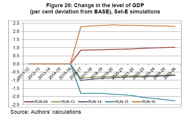 Employment levels in these scenarios follow the movements in GDP. In RUN-13, RUN-14, and RUN-15, the level of employment falls below BASE levels implying unemployment occurs in these three scenarios (Table 13). In RUN-16, however, employment expands significantly more than BASE levels. Interestingly, this is the only scenario across all the sets where employment generation is highest for unskilled labour, followed by semi-skilled and skilled labour in that order. In Table 13 we present the model outcomes on some key variables that would help understand the above result on the GDP impacts. Looking first at RUN-13 and RUN-14 where we specify that the government imposes additional direct taxes on top 30 per cent of rural and urban households, we see that direct tax collection rises significantly compared to BASE. In 2016-17, it rises by nearly 41 per cent over the BASE level. Over time the percentage rise in tax collection over BASE level comes down somewhat though it is still a whopping 35 per cent in the terminal year. Consequently, the total revenue of the government rises dramatically by about 19 per cent in 2016-17, though the percentage rise comes down somewhat over time. With government consumption kept constant in real terms at BASE levels in these two simulations, the rise in government revenue translates into a sharp reduction in government dis-savings by about 60 per cent to 69 per cent over the years. The additional taxes, however, has adverse impacts on the savings and consumption of the top 30 per cent of households and consequently aggregate private consumption (3 per cent to 3.5 per cent) and private savings (5.5 per cent to 6.7 per cent) are lower in these two simulations. With the fall in private consumption aggregate domestic demand is lower in these 2 simulations than in BASE by 20 to 50 basis points. Aggregate domestic demand being lower is the reason that GDP is lower in these two simulations than in BASE as seen earlier in Figure 26. | Table 13: Set-E simulations (percentage change from BASE) | | Variable | 2016-17 | 2017-18 | 2018-19 | 2019-20 | 2020-21 | 2021-22 | 2022-23 | 2023-24 | 2024-25 | 2025-26 | | Unskilled labour employment | | RUN-13 | -0.3 | -0.1 | -0.1 | 0.0 | 0.0 | 0.0 | 0.0 | 0.1 | 0.1 | 0.1 | | RUN-14 | -0.4 | -0.2 | -0.1 | -0.1 | -0.1 | 0.0 | 0.0 | 0.0 | 0.0 | 0.1 | | RUN-15 | -0.4 | -0.3 | -0.3 | -0.3 | -0.3 | -0.3 | -0.3 | -0.3 | -0.3 | -0.4 | | RUN-16 | 2.9 | 2.9 | 3.1 | 3.2 | 3.4 | 3.6 | 3.7 | 3.8 | 4.0 | 4.2 | | Semi-skilled labour employment | | RUN-13 | -0.7 | -0.6 | -0.5 | -0.4 | -0.4 | -0.3 | -0.3 | -0.3 | -0.2 | -0.2 | | RUN-14 | -0.9 | -0.7 | -0.6 | -0.5 | -0.5 | -0.4 | -0.4 | -0.3 | -0.3 | -0.3 | | RUN-15 | -1.2 | -1.1 | -1.1 | -1.1 | -1.0 | -1.0 | -1.1 | -1.1 | -1.1 | -1.1 | | RUN-16 | 2.4 | 2.4 | 2.5 | 2.6 | 2.7 | 2.9 | 3.0 | 3.1 | 3.2 | 3.3 | | Skilled labour employment | | RUN-13 | -1.9 | -1.7 | -1.6 | -1.5 | -1.4 | -1.4 | -1.4 | -1.3 | -1.2 | -1.2 | | RUN-14 | -2.0 | -1.8 | -1.7 | -1.6 | -1.5 | -1.4 | -1.4 | -1.3 | -1.3 | -1.2 | | RUN-15 | -3.8 | -3.7 | -3.6 | -3.6 | -3.6 | -3.6 | -3.7 | -3.7 | -3.8 | -3.9 | | RUN-16 | 0.8 | 0.7 | 0.7 | 0.6 | 0.5 | 0.4 | 0.3 | 0.3 | 0.2 | 0.2 | | Direct tax revenue | | RUN-13 | 40.6 | 38.2 | 36.4 | 35.9 | 35.0 | 35.0 | 36.0 | 35.0 | 35.0 | 34.9 | | RUN-14 | 41.1 | 38.6 | 36.7 | 36.1 | 35.1 | 35.1 | 36.0 | 35.1 | 35.0 | 34.9 | | RUN-15 | -1.9 | -1.7 | -1.6 | -1.5 | -1.4 | -1.4 | -1.4 | -1.5 | -1.5 | -1.5 | | RUN-16 | 2.4 | 2.6 | 2.7 | 2.9 | 3.0 | 3.1 | 3.2 | 3.2 | 3.3 | 3.4 | | Government total revenue | | RUN-13 | 19.3 | 18.5 | 17.7 | 17.8 | 17.5 | 17.4 | 16.7 | 15.2 | 14.8 | 14.4 | | RUN-14 | 19.5 | 18.6 | 17.8 | 17.8 | 17.5 | 17.5 | 16.7 | 15.2 | 14.8 | 14.3 | | RUN-15 | -1.8 | -1.7 | -1.7 | -1.7 | -1.6 | -1.7 | -2.4 | -3.1 | -3.4 | -3.8 | | RUN-16 | 2.2 | 2.3 | 2.3 | 2.4 | 2.5 | 2.5 | 1.8 | 1.1 | 0.8 | 0.5 | | Government consumption | | RUN-13 | 0.4 | 0.4 | 0.3 | 0.3 | 0.3 | 0.3 | 0.3 | 0.3 | 0.3 | 0.2 | | RUN-14 | 0.4 | 0.4 | 0.3 | 0.3 | 0.3 | 0.3 | 0.3 | 0.3 | 0.3 | 0.2 | | RUN-15 | -18.7 | -18.3 | -18.3 | -18.4 | -18.5 | -18.8 | -19.2 | -19.5 | -19.8 | -20.2 | | RUN-16 | -9.9 | -10.6 | -11.5 | -12.3 | -13.5 | -14.5 | -15.1 | -16.1 | -16.9 | -17.9 | | Government dis-savings | | RUN-13 | 68.0 | 65.5 | 63.7 | 59.8 | 59.2 | 59.7 | 61.8 | 65.5 | 64.9 | 65.9 | | RUN-14 | 68.7 | 65.9 | 63.9 | 60.0 | 59.2 | 59.7 | 61.8 | 65.4 | 64.7 | 65.7 | | RUN-15 | 41.9 | 41.7 | 41.6 | 39.9 | 40.1 | 40.7 | 42.6 | 46.7 | 47.0 | 48.3 | | RUN-16 | 35.5 | 38.4 | 41.1 | 41.3 | 44.6 | 47.4 | 50.8 | 58.2 | 60.5 | 64.3 | | Private consumption | | RUN-13 | -3.4 | -3.3 | -3.2 | -3.2 | -3.2 | -3.2 | -3.4 | -3.3 | -3.4 | -3.4 | | RUN-14 | -3.5 | -3.4 | -3.3 | -3.3 | -3.3 | -3.3 | -3.4 | -3.4 | -3.4 | -3.4 | | RUN-15 | -0.9 | -0.9 | -0.9 | -0.9 | -0.9 | -0.9 | -1.0 | -1.0 | -1.0 | -1.0 | | RUN-16 | 2.1 | 2.2 | 2.2 | 2.3 | 2.4 | 2.5 | 2.5 | 2.6 | 2.7 | 2.8 |
| Table 13: Set-E simulations (percentage change from BASE) (Contd.) | | Variable | 2016-17 | 2017-18 | 2018-19 | 2019-20 | 2020-21 | 2021-22 | 2022-23 | 2023-24 | 2024-25 | 2025-26 | | Private savings | | RUN-13 | -6.4 | -6.1 | -5.8 | -5.7 | -5.5 | -5.5 | -5.6 | -5.5 | -5.5 | -5.5 | | RUN-14 | -6.7 | -6.3 | -5.9 | -5.8 | -5.6 | -5.6 | -5.7 | -5.6 | -5.6 | -5.5 | | RUN-15 | -1.4 | -1.4 | -1.3 | -1.3 | -1.3 | -1.3 | -1.3 | -1.3 | -1.3 | -1.2 | | RUN-16 | 3.0 | 3.0 | 3.0 | 3.0 | 3.0 | 3.1 | 3.2 | 3.2 | 3.3 | 3.4 | | Aggregate domestic demand | | RUN-13 | -0.3 | -0.3 | -0.3 | -0.3 | -0.3 | -0.3 | -0.3 | -0.2 | -0.2 | -0.2 | | RUN-14 | -0.5 | -0.4 | -0.4 | -0.4 | -0.3 | -0.3 | -0.3 | -0.3 | -0.3 | -0.3 | | RUN-15 | -0.8 | -0.8 | -0.8 | -0.8 | -0.8 | -0.8 | -0.9 | -0.9 | -0.9 | -0.9 | | RUN-16 | 2.7 | 2.8 | 2.8 | 2.9 | 3.0 | 3.0 | 3.1 | 3.2 | 3.2 | 3.3 | | Exports (% of GDP) | | RUN-13 | 0.5 | 0.4 | 0.4 | 0.4 | 0.3 | 0.3 | 0.3 | 0.3 | 0.3 | 0.2 | | RUN-14 | 0.4 | 0.4 | 0.3 | 0.3 | 0.3 | 0.3 | 0.3 | 0.2 | 0.2 | 0.2 | | RUN-15 | -1.3 | -1.3 | -1.3 | -1.3 | -1.3 | -1.3 | -1.4 | -1.4 | -1.4 | -1.4 | | RUN-16 | 1.5 | 1.7 | 1.7 | 1.8 | 1.9 | 1.9 | 2.0 | 2.1 | 2.1 | 2.2 | | Imports (% of GDP) | | RUN-13 | 0.6 | 0.5 | 0.4 | 0.4 | 0.4 | 0.3 | 0.3 | 0.3 | 0.3 | 0.3 | | RUN-14 | 0.7 | 0.6 | 0.5 | 0.5 | 0.5 | 0.4 | 0.4 | 0.4 | 0.3 | 0.3 | | RUN-15 | -0.9 | -1.0 | -1.0 | -1.0 | -1.0 | -1.0 | -1.1 | -1.1 | -1.1 | -1.2 | | RUN-16 | -3.6 | -3.8 | -4.0 | -4.2 | -4.5 | -4.8 | -5.0 | -5.2 | -5.5 | -5.7 | | Current a/c deficit (% of GDP) | | RUN-13 | 0.8 | 0.7 | 0.7 | 0.6 | 0.6 | 0.5 | 0.5 | 0.4 | 0.4 | 0.4 | | RUN-14 | 4.1 | 3.2 | 2.9 | 2.6 | 2.4 | 2.2 | 2.0 | 1.9 | 1.6 | 1.5 | | RUN-15 | 3.8 | 2.9 | 2.5 | 2.3 | 2.2 | 2.0 | 1.9 | 1.8 | 1.5 | 1.4 | | RUN-16 | -88.8 | -77.7 | -78.0 | -76.6 | -81.3 | -85.8 | -87.2 | -93.5 | -91.5 | -98.8 | | Exchange rate (2011-12 = 100) | | RUN-13 | 0.2 | 0.2 | 0.1 | 0.1 | 0.1 | 0.1 | 0.1 | 0.1 | 0.1 | 0.1 | | RUN-14 | 0.0 | 0.0 | 0.0 | 0.0 | 0.0 | 0.0 | 0.0 | 0.0 | 0.0 | 0.0 | | RUN-15 | 0.0 | 0.0 | 0.0 | 0.0 | 0.0 | 0.0 | 0.0 | 0.0 | 0.0 | 0.0 | | RUN-16 | 5.0 | 5.3 | 5.5 | 5.8 | 6.1 | 6.3 | 6.6 | 6.9 | 7.1 | 7.4 | | Foreign savings | | RUN-13 | 0.2 | 0.2 | 0.1 | 0.1 | 0.1 | 0.1 | 0.1 | 0.1 | 0.1 | 0.1 | | RUN-14 | 3.2 | 2.5 | 2.2 | 2.0 | 1.8 | 1.7 | 1.6 | 1.5 | 1.3 | 1.2 | | RUN-15 | 4.5 | 3.6 | 3.3 | 3.1 | 3.0 | 2.9 | 2.8 | 2.8 | 2.5 | 2.4 | | RUN-16 | -88.4 | -76.9 | -77.1 | -75.6 | -80.5 | -85.1 | -86.6 | -93.2 | -91.0 | -98.7 | | Source: Authors’ calculations | The impact of the difference in the closure for foreign exchange market between RUN-13 and RUN-14 needs to be noted. In RUN-13 where the foreign capital flows is fixed at BASE level, the exchange rate depreciates slightly by about 10 basis points. Whereas in RUN-14, where the exchange rate is kept fixed at BASE level, the CAD jumps up sharply in 2016-17 over the BASE level and thereafter this difference narrows down somewhat. The rise in investments generates additional import demand, which is the main driver of the rise in CAD in RUN-14. Additionally, the rise in import competition also adds to the reduction in output seen earlier, which results in lower exports in this simulation. Consequently, the rise in CAD results only in a small rise in foreign savings, and thus does not help reduce the additional tax burden on households. Turning to RUN-15 and RUN-16 we find that the impact of cut in the government consumption to generate the requisite savings to meet the investment target depends crucially on the exchange rate. In RUN-15 where we set the exchange rate at the BASE level, government has to cut its consumption expenditure by 18 per cent to 20 per cent over the years. Whereas in RUN-16, by allowing the Rupee to depreciate by 5 per cent in the first year of the shock (2016-17) the cut in government consumption expenditure required is only 10 per cent over BASE levels. But since the depreciation in the Rupee is restricted to only a quarter per cent annually from 2017-18 onwards we see that a larger and increasing amount of cut in government consumption expenditure is required to meet the investment target. To understand this further, it must be noted that in these two simulations (RUN-15 and RUN-16) there are no additional taxes on households, and government transfers and foreign remittances are also kept fixed in real terms at BASE levels. Consequently, household savings and consumption essentially reflect the changes in aggregate GDP from which households derive their income to a very large part. Thus, changes in private savings/ private consumption do not drive the results in these two simulations. The drivers are really the trade flows and foreign savings. The depreciation of the Rupee in RUN-16 helps expand exports (by 1.5 per cent to 2.2 per cent over time) and cut down on imports (3.5 per cent to nearly 6 per cent) due to which the CAD improves dramatically. Indeed, in 2016-17 the CAD as a percentage of GDP declines by 89 per cent over BASE levels, and falls thereafter such that by the terminal year the CAD is nearly entirely wiped out compared to BASE, which is reflected in foreign savings also. The fall in imports in RUN-16 shifts the demand in favour of domestic production and this is seen in the aggregate domestic demand rising by 3 per cent despite the fall in government consumption in this simulation. This coupled with the rise in exports catalyses the expansion in domestic production and consequently aggregate GDP expands in this simulation as seen earlier in Figure 26. In RUN-15, where the exchange rate is higher than in RUN-16, none of these favourable effects take place. Indeed, the rate is high enough to adversely affect exports and favour imports, and this eventually affects domestic production and aggregate GDP. 5 Conclusions In this study we examine the impacts of various types of government expenditure on the Indian economy. In particular, we examine the impacts of a rise in (a) Government consumption expenditure in general and the nature of the relation between government expenditure and GDP, (b) Government expenditure in Social Sectors and in Public Administration, (c) Government transfer payments to households, and (d) Public investment. Towards this, we have used a recursively dynamic CGE model of the Indian economy developed by Bhakta and Ganesh-Kumar (2016), which is built around SAM for the year 2011-12. The SAM and the model distinguish 9 commodities/ sectors, 9 factors of production, and 12 household types distinguished by their location and by the MPCE percentile. The model is solved annually over the period 2011-12 to 2025-26. This 15 year simulation period can be categorised into (a) the historic period covering the 5 years 2011-12 to 2015-16 for which the model replicates as closely as possible the actual observed values of key macroeconomic variables (annual growth in aggregate and sectoral GDPs, exports and imports, the shares of agriculture, manufacturing and services in total GDP, and the share of exports, imports and trade deficit in GDP), and (b) the future 10-year period from 2016-17 to 2025-26 over which various alternative scenarios are developed. As a first step, we develop a BASE scenario that captures a “Business As Usual” trajectory that the Indian economy is likely to take over the 10-year period 2016-17 to 2025-26 given the current structural characteristics of the economy, and the set of policies currently prevailing. Following an assessment of the available forecasts of the future growth of the economy from diverse sources such as the Government of India, Reserve Bank of India, the IMF, the UN and the World Bank, we develop the BASE scenario such that the growth rate of the economy improves steadily in the next couple of years and reaches a steady state growth rate of 8.5 per cent per annum from 2017-18 onwards. We then develop various counter-factual policy scenarios by introducing a ‘policy shock’ starting from the year 2016-17. The policy shock typically involves changing the values of specific parameter(s) that represent a certain government policy combined with a particular specification of macroeconomic closure of the model. The macroeconomic closure describes the functioning/ determination of (a) the factor markets, (b) foreign exchange market, and (c) savings-investment in the economy. In all we develop five sets of counter-factual policy scenarios to study the economy-wide impacts of different types of public expenditure. Each of these sets consists of two or more simulations that are designed to address one main question and its sub-questions, if any. In what follows we first summarise our findings against each of these five main questions: What are the impacts of a rise in government consumption expenditure? In the first set of 4 simulations, we increase government consumption expenditure in each year by 10 per cent starting from 2016-17 over the corresponding level in the BASE scenario. The 4 simulations (RUN-01 to RUN-04) capture alternative combinations of macroeconomic conditions relating to factor and foreign exchange markets. The results show that impact on the level and growth rate of GDP depends crucially upon the macroeconomic conditions prevailing in the economy when the fiscal expansion is undertaken, in particular, whether there are unemployed factors to start with or if the economy is already under full employment. When there are unemployed factors in the economy (RUN-02 and RUN-04) such as during a downturn a short-term boost to both the level and growth rate of GDP is seen in the first year when fiscal expansion takes place. The level of GDP rises by 0.8 per cent over BASE levels in 2016-17 and this difference rises gradually to about 1 per cent in the terminal year. The growth rate of GDP also rises to about 9.1 per cent in 2016-17, but thereafter settles back roughly to the level in BASE scenario. In contrast when fiscal expansion is undertaken amidst full employment of all factors, the level of GDP declines immediately and continues to fall dramatically over time. The amount of fall in GDP and its growth rate depends crucially upon whether foreign capital is willing to sustain fiscal expansion or not. When foreign capital is forthcoming (RUN-01), the level of GDP is 3.8 per cent lower than in BASE in the terminal year, and the terminal year growth rate is just 7.7 per cent compared to 8.5 per cent in BASE. The corresponding figures in the case when foreign capital is not forthcoming (RUN-03) are 7.9 per cent and 6.3 per cent, respectively. When fiscal expansion happens under conditions of full employment (RUN-01 and RUN-03), the initial impact on domestic production and GDP is not much. However, with resources getting diverted to current consumption, government dis-savings become even larger, which adversely affects investment and future growth. And this adverse impact on growth increases over time. The fall in domestic production in turn adversely affects export supply and hence the trade and current account deficit. And in such a situation if foreign capital is not forthcoming, as is reasonable to expect, it results in massive depreciation of the currency (RUN-03). The presence of unemployed factors in RUN-02 and RUN-04 makes it possible to expand employment and output, which has beneficial impacts on household income, consumption and savings and also generates both tax and non-tax revenue for the government. As a result, private savings is higher in this case and government dis-savings do not rise as dramatically as under full employment conditions. Consequently, investment levels are higher in the unemployment case resulting in higher GDP. The results also show that in a situation where unemployed factors exist, whether or not foreign capital is supportive of fiscal expansion for current consumption hardly matters to the final outcome. Indeed, even if foreign capital flow remains tight, the exchange rate remains fairly stable due to higher export made possible by output expansion. What is the nature of the relationship between government expenditure and GDP? The second set of simulations is similar in construct to RUN-04 of the first set, except for the quantum of increase in government expenditure. Along with RUN-04, the four alternative simulations (RUN-05 to RUN-08) that we have tried here allow us to study the impact of increase in government expenditure ranging from 5 per cent to 25 per cent in steps of 5 percentage points. The simulation results suggest that the relationship between government expenditure and GDP is fairly linear. In the first year after the shock is introduced, the level of GDP rises by roughly 0.4 per cent to 0.5 per cent over the BASE level for every 5 percentage point increase in government expenditure across these simulations including RUN-04. In the subsequent years too, the difference in the GDP level across these simulations is more or less of a similar order. As the difference in the level of GDP across these simulations is nearly constant, it suggests a fairly linear relationship between government expenditure and GDP. This is also borne out in terms of GDP growth rates, which shows variations across the simulations only in the first year, but is virtually same as in BASE in all these simulations in the later years, suggesting that differences in the quantum of government expenditure causes only a level shift in GDP but leaves the growth trajectory unchanged. It is worth noting here that we have deduced the linear relationship between government expenditure and GDP based on a detailed CGE model in which most of the equations that characterise production, consumption, trade, income distribution across factors and agents of the economy, and various government policies, are all non-linear. Further, it is worth stressing that GDP in our model is itself computed by aggregating sectoral value added, which is endogenously determined based on demand and supply conditions faced by individual sectors as well as in the factor markets, which affect both product and factor prices and hence returns to factors, all of which are endogenous in the model. What are the impacts of a rise in government consumption expenditure in specific sectors? In the two simulations in this set (RUN-09 and RUN-10), we study the impact of increasing government expenditure in specific sectors, viz., social sectors (water supply, education and medical services) in RUN-09 and Public Administration in RUN-10. We maintain the same quantum of increase in the government expenditure as well as the macroeconomic closure as in RUN-04. The results show that in terms of the level of GDP focusing additional government expenditure on particular sectors does not have any significant extra impact compared to the case when the additional expenditure is broad-based. The additional GDP in these simulations over RUN-04 in 2016-17 is just 20 basis points. Though the GDP increase in the later years is slightly more, nevertheless the difference is not very large. Indeed, the similarity of results in these two simulations with RUN-04 is seen in several other macro variables of interest such as gross fixed capital formation, various expenditure categories as a percentage of GDP, sectoral shares in aggregate GDP, sectoral relative prices, and real income per capita of households. It is only the level of government dis-savings that shows a somewhat large difference compared to its level in RUN-04. But this hardly has any impact on aggregate GDP due to the small adjustments that are spread out across several variables in the economy. Thus, our results point out that given the current structure of inter-industry linkages as captured in the SAM, focusing additional GDP on social sectors or on public administration does not affect GDP growth. The impacts, if any, of such targeted expenditure on social sectors has to be measured in terms of non-economic indicators pertaining to health, education, water and sanitation, etc. These non-economic indicators are beyond the scope of our model. What are the impacts of a rise in government transfers to households? The fourth set consists of two simulations wherein instead of spending on its current consumption, the government transfers an equivalent amount either to all households (RUN-11) or to the bottom 70 per cent of households in rural and urban areas (RUN-12). We keep the same macroeconomic closures in these two simulations as in RUN-04. We find that additional transfers to households results in much less rise in the level of GDP than when the government spends the same amount on its current consumption. In these simulations, GDP in 2011-12 rises by about 30 basis points over BASE as against 85 basis points increase in RUN-04. Moreover, the additional GDP in RUN-11 and RUN-12 over BASE levels actually declines over time whereas in RUN-04 it rises. The result also shows that the outcomes for the two simulations do not vary much amongst themselves, in the level and growth in GDP and also in terms of several other macroeconomic variables of interest such as real income per capita of households, private savings, various types of final expenditure, exchange rate, etc. Government dis-saving in these simulations is higher than in RUN-04 by about 4.1 per cent to 9.7 per cent over time suggesting that the fiscal resource position in these simulations is relatively weaker than in RUN-04. The rise in the level of government dis-saving in these simulations dominates over the rise in private savings seen earlier, and consequently capital formation in the economy is somewhat lower than in RUN-04, and this shortfall is seen to rise over time. The main driver for this result is the difference in the consumption pattern of households and government and its cascading on production, employment, and value added. In both these simulations household demand for agricultural and industrial products and services is higher compared to RUN-04. However, total demand is higher for both agricultural and industrial products and lower only for services. While household demand is relatively more for agricultural and industrial products, government demand is relatively more for services. As a result, total demand for agricultural and industrial products expands triggering an expansion in the output of these two sectors. Given the relative dominance of services in the economy, aggregate GDP does not expand as much in these simulations as in RUN-04. The lower aggregate GDP in these simulations than in RUN-04 in turn results in lower direct tax revenue for the government and hence the weaker fiscal position as reflected in the higher government dis-savings, which eventually affects the level of investment and future GDP growth. What are the impacts of a rise in government investment expenditure? To study this question, we first of all change the savings-investment closure in the model. In the 4 simulations (RUN-13 to RUN-16) that make this final set, we keep the investment fixed at an elevated level than in BASE to reflect the increase in government investment by an amount equal to the increase in government consumption expenditure in RUN-04. The 4 simulations in this set differ among themselves in the way the requisite savings is generated to meet this ‘investment target’. In RUN-13 and RUN-14 we introduce a variable rate of direct tax applicable on the top 30 per cent of the households in both rural and urban areas in order to raise government’s revenue and hence its savings. In RUN-15 and RUN-16 we consider the case of government cutting down its current expenditure in order to raise its savings. In RUN-13, we keep the level of foreign capital flows fixed at BASE levels and determine the exchange rate endogenously, while in the remaining three simulations we do the converse to allow for the possibility that foreign capital flows could be accommodative of rise in government investment. In RUN-14 and RUN-15 we keep the exchange rate fixed at BASE level while in RUN-16 we allow the Rupee to depreciate somewhat (5 per cent over BASE levels in 2016-17 and 0.25 per cent annually thereafter). Our simulations show that the impact on GDP varies dramatically both in terms of magnitude and direction depending upon the way resources required to meet the targeted level of investment is generated. Compared with BASE, the level of GDP falls when the government levies additional taxes on the top 30 per cent of the households as in RUN-13 and RUN-14. This happens irrespective of whether or not foreign capital is supportive of expansion of public investments. But when the government opts for a cut in current consumption to finance the additional public investment, then the impact on the level of GDP depends crucially on the level of exchange rate. When the exchange rate is kept fixed at BASE level (RUN-15) GDP falls by about two percentage points. But when the currency is allowed to depreciate (RUN-16), the level of GDP actually rises by 2 per cent to 2.5 per cent over the years. When government imposes additional taxes on households, while its revenue rise and its dis-savings fall, it adversely affects private savings and consumption. The net result is a reduction in aggregate demand, which drives down output and GDP. Here additional foreign capital flows is not helpful. The ensuing rise in CAD is accompanied by a rise in imports, and this additional import competition also edges out domestic output at the margin. When government cuts its consumption to raise its savings, the result again is a net reduction in aggregate demand and hence output when the exchange rate is kept fixed at BASE levels. But when the Rupee is allowed to depreciate somewhat it propels expansion of exports and also shifts some of the domestic demand away from imports in favour of domestic production due to which the amount by which government has to cut its consumption reduces. All these result in an expansion of aggregate demand and hence output. Overall conclusions: To sum up, the impact of expansion in government expenditure across different types of expenditure depends first of all on the nature of expenditure undertaken. More crucially it depends upon the prevailing macroeconomic conditions, especially whether there is full employment/ unemployment of factors, and also on the complementary set of policies that are needed to generate the resources required to finance the additional expenditure. The main messages that emerge from this study are as follows: -
Fiscal expansion in boom times is actually disastrous for the economy on all counts. -
However, it is not a foregone conclusion that fiscal expansion during recessionary conditions when unemployment prevails is always beneficial. It depends crucially on the type of government expenditure undertaken and the accompanying set of policies that determine how fiscal expansion is financed. -
Amongst alternative types of current expenditure, clearly expansion of government consumption scores over additional transfers to households in terms of impact on GDP. -
Between additional government current consumption and investment, the choice is not straightforward. -
Using additional taxes on households to finance expansion of public investment does not fare well compared to government consumption. -
Nor does shifting of government expenditure from current consumption to investment help if the exchange rate regime is neutral. -
Amongst all the policy options considered in this study, shifting of government expenditure from current consumption to investments accompanied by a slight depreciation of the Rupee turns out to be the best in terms of overall impacts on the GDP and various other macro indicators as well as household real income per capita. At the end, some limitations of the study need to be noted. The study is based on SAM for the year 2011-12. Two crucial limitations of this SAM need to be noted. First, the SAM used here was originally constructed using the NAS at 2004-05 prices, which we then rescaled and tweaked to reflect the broad structure of the economy as reflected in the NAS data at 2011-12 prices for use in this SAM in the study. While doing so, we have focused primarily at the shares of the three broad sectors of the economy in GDP and share of trade flows. A clearly better option would have been to construct a SAM from scratch using the NAS data at 2011-12 prices. We could not do this as at the time the study was commenced information on all variables required to construct the SAM was not available in the New Series of NAS data. Second, even in the SAM that we currently have, the input-output transaction flows do not exactly correspond to the base year 2011-12. They are in fact based on the Input-Output Table for 2007-08 published by the CSO suitably recalibrated. The only reason for this is the non-availability of an IO Table for 2011-12 at the time of commencing this study. It is also for this reason that the sectoral detail that we have in the study is also very limited, which probably explains why the Set-C simulations on focusing government expenditure on specific sectors do not generate interesting results. Again, the best option would be to use an IO Table for 2011-12. It is only very recently when this study was drawing to a close that the CSO has brought out a Supply-Use Table for 2011-12. This opens the possibility for a later study to overcome some of these data driven limitations.
Reference Bhakta. R. (2015). “Educational Attainment of Young Adults in India: Measures, Trends & Determinants”. WP-2015-034. Indira Gandhi Institute of Development Research, Mumbai. Bhakta, R. and A. Ganesh-Kumar (2016). “Adult education, labour market outcomes and their Implications for income distribution in India: An Analysis using a CGE model”. Paper presented at the 24th International Input-Output Association (IIOA) Conference, Yonsei University, Seoul, 03-08 July, 2016. Dervis, K., J. de Melo and S. Robinson (1982). General Equilibrium Models for Development Policy. Cambridge University Press, Cambridge. Ganesh-Kumar, A. (2015). “A Social Accounting Matrix for India, 2011-12”. Unpublished mimeo. Indira Gandhi Institute of Development Research, Mumbai. Ganesh-Kumar, A. and M. Panda (2009). “Global Economic Shocks and Indian Policy Response: An Analysis Using a CGE model”. In K. S. Parikh (Ed.) Macro-Modeling for the Eleventh Five Year Plan of India, Planning Commission, Government of India/ Academic Foundation, New Delhi. Johansen, L. (1960). A Multi-Sectoral Study of Economic Growth. North Holland, Amsterdam. Mathias D. and G. Michel (1987). “On closure rules, homogeneity and dynamics in applied general equilibrium models”. Journal of Development Economics, Vol. 26. Planning Commission (2008). Report of the Working Group on Labour Force & Employment Projections constituted for the Eleventh Five Year Plan (2007 – 2012). Planning Commission, Government of India, New Delhi. Pradhan, B. K., M. R. Saluja, and A. Sahoo (2001). Social Accounting Matrix for India 1997–98: Concepts, Constructions and Applications. National Council of Applied Economic Research, New Delhi. Rattso, J. (1982). “Different macroclosures of the original Johansen model and their impact on policy evaluation”. Journal of Policy Modeling, Vol. 4. Saluja, M.R. and B. Yadav (2006). Social Accounting Matrix for India 2003-04. India Development Foundation, Gurgaon. Sen, A. K. (1963). “Neo-Classical and Neo-Keynesian Theories of Distribution”. Economic Record 39, pp.54-64. UN-DESA-PD (2014). World Urbanization Prospects: The 2014 Revision, CD-ROM Edition, United Nations, Department of Economic and Social Affairs, Population Division.
Appendix 1: Social Accounting Matrix for 2011-12 | National SAM at Market Prices, 2011-12, Rs.Crores | | | Commodity | Activity | | C-AGRI | C-MANUF1 | C-MANUF2 | C-ELEC | C-WATER | C-EDUCATION | C-MEDICAL | C-SRVS1 | C-SRVS2 | A-AGRI | A-MANUF1 | A-MANUF2 | A-ELEC | A-WATER | | Commodity | C-AGRI | 0 | 0 | 0 | 0 | 0 | 0 | 0 | 0 | 0 | 395776 | 655164 | 13164 | 520 | 0 | | | C-MANUF1 | 0 | 0 | 0 | 0 | 0 | 0 | 0 | 0 | 0 | 74081 | 2572407 | 1217696 | 32839 | 3156 | | | C-MANUF2 | 0 | 0 | 0 | 0 | 0 | 0 | 0 | 0 | 0 | 156998 | 523085 | 1721743 | 55048 | 1497 | | | C-ELEC | 0 | 0 | 0 | 0 | 0 | 0 | 0 | 0 | 0 | 23144 | 88432 | 42989 | 77500 | 671 | | | C-WATER | 0 | 0 | 0 | 0 | 0 | 0 | 0 | 0 | 0 | 694 | 13178 | 1596 | 1063 | 13042 | | | C-EDUCATION | 0 | 0 | 0 | 0 | 0 | 0 | 0 | 0 | 0 | 389 | 16565 | 0 | 0 | 0 | | | C-MEDICAL | 0 | 0 | 0 | 0 | 0 | 0 | 0 | 0 | 0 | 0 | 0 | 0 | 0 | 0 | | | C-SRVS1 | 0 | 0 | 0 | 0 | 0 | 0 | 0 | 0 | 0 | 264791 | 970149 | 271474 | 22745 | 5496 | | | C-SRVS2 | 0 | 0 | 0 | 0 | 0 | 0 | 0 | 0 | 0 | 25774 | 159238 | 86493 | 8832 | 1666 | | Activity | A-AGRI | 2440754 | 0 | 0 | 0 | 0 | 0 | 0 | 0 | 0 | 0 | 0 | 0 | 0 | 0 | | | A-MANUF1 | 0 | 6859270 | 0 | 0 | 0 | 0 | 0 | 0 | 0 | 0 | 0 | 0 | 0 | 0 | | | A-MANUF2 | 0 | 0 | 4034980 | 0 | 0 | 0 | 0 | 0 | 0 | 0 | 0 | 0 | 0 | 0 | | | A-ELEC | 0 | 0 | 0 | 328203 | 0 | 0 | 0 | 0 | 0 | 0 | 0 | 0 | 0 | 0 | | | A-WATER | 0 | 0 | 0 | 0 | 60163 | 0 | 0 | 0 | 0 | 0 | 0 | 0 | 0 | 0 | | | A-EDUCATION | 0 | 0 | 0 | 0 | 0 | 316903 | 0 | 0 | 0 | 0 | 0 | 0 | 0 | 0 | | | A-MEDICAL | 0 | 0 | 0 | 0 | 0 | 0 | 176846 | 0 | 0 | 0 | 0 | 0 | 0 | 0 | | | A-SRVS1 | 0 | 0 | 0 | 0 | 0 | 0 | 0 | 2589090 | 0 | 0 | 0 | 0 | 0 | 0 | | | A-SRVS2 | 0 | 0 | 0 | 0 | 0 | 0 | 0 | 0 | 2606757 | 0 | 0 | 0 | 0 | 0 | | Factors | L-UNSK | 0 | 0 | 0 | 0 | 0 | 0 | 0 | 0 | 0 | 637874 | 327593 | 3203 | 402 | 817 | | | L-SMSK | 0 | 0 | 0 | 0 | 0 | 0 | 0 | 0 | 0 | 431969 | 216115 | 8314 | 916 | 587 | | | L-SKLD | 0 | 0 | 0 | 0 | 0 | 0 | 0 | 0 | 0 | 49042 | 22959 | 10236 | 961 | 120 | | | K-AGRI | 0 | 0 | 0 | 0 | 0 | 0 | 0 | 0 | 0 | 380222 | 0 | 0 | 0 | 0 | | | K-INDY | 0 | 0 | 0 | 0 | 0 | 0 | 0 | 0 | 0 | 0 | 1294386 | 658072 | 127379 | 0 | | | K-WATER | 0 | 0 | 0 | 0 | 0 | 0 | 0 | 0 | 0 | 0 | 0 | 0 | 0 | 33110 | | | K-EDUCATION | 0 | 0 | 0 | 0 | 0 | 0 | 0 | 0 | 0 | 0 | 0 | 0 | 0 | 0 | | | K-MEDICAL | 0 | 0 | 0 | 0 | 0 | 0 | 0 | 0 | 0 | 0 | 0 | 0 | 0 | 0 | | | K-SRVS | 0 | 0 | 0 | 0 | 0 | 0 | 0 | 0 | 0 | 0 | 0 | 0 | 0 | 0 | | Households | RH-D0010 | 0 | 0 | 0 | 0 | 0 | 0 | 0 | 0 | 0 | 0 | 0 | 0 | 0 | 0 | | | RH-D1030 | 0 | 0 | 0 | 0 | 0 | 0 | 0 | 0 | 0 | 0 | 0 | 0 | 0 | 0 | | | RH-D3050 | 0 | 0 | 0 | 0 | 0 | 0 | 0 | 0 | 0 | 0 | 0 | 0 | 0 | 0 | | | RH-D5070 | 0 | 0 | 0 | 0 | 0 | 0 | 0 | 0 | 0 | 0 | 0 | 0 | 0 | 0 | | | RH-D7090 | 0 | 0 | 0 | 0 | 0 | 0 | 0 | 0 | 0 | 0 | 0 | 0 | 0 | 0 | | | RH-D90100 | 0 | 0 | 0 | 0 | 0 | 0 | 0 | 0 | 0 | 0 | 0 | 0 | 0 | 0 | | | UH-D0010 | 0 | 0 | 0 | 0 | 0 | 0 | 0 | 0 | 0 | 0 | 0 | 0 | 0 | 0 | | | UH-D1030 | 0 | 0 | 0 | 0 | 0 | 0 | 0 | 0 | 0 | 0 | 0 | 0 | 0 | 0 | | | UH-D3050 | 0 | 0 | 0 | 0 | 0 | 0 | 0 | 0 | 0 | 0 | 0 | 0 | 0 | 0 | | | UH-D5070 | 0 | 0 | 0 | 0 | 0 | 0 | 0 | 0 | 0 | 0 | 0 | 0 | 0 | 0 |
| National SAM at Market Prices, 2011-12, Rs.Crores | | | Commodity | Activity | | C-AGRI | C-MANUF1 | C-MANUF2 | C-ELEC | C-WATER | C-EDUCATION | C-MEDICAL | C-SRVS1 | C-SRVS2 | A-AGRI | A-MANUF1 | A-MANUF2 | A-ELEC | A-WATER | | | UH-D7090 | 0 | 0 | 0 | 0 | 0 | 0 | 0 | 0 | 0 | 0 | 0 | 0 | 0 | 0 | | | UH-D90100 | 0 | 0 | 0 | 0 | 0 | 0 | 0 | 0 | 0 | 0 | 0 | 0 | 0 | 0 | | Enterprises | PVT-ENT | 0 | 0 | 0 | 0 | 0 | 0 | 0 | 0 | 0 | 0 | 0 | 0 | 0 | 0 | | | PUB-ENT | 0 | 0 | 0 | 0 | 0 | 0 | 0 | 0 | 0 | 0 | 0 | 0 | 0 | 0 | | Government | TXDIR | 0 | 0 | 0 | 0 | 0 | 0 | 0 | 0 | 0 | 0 | 0 | 0 | 0 | 0 | | | TARIFF | 673 | 53004 | 55793 | 0 | 0 | 0 | 0 | 0 | 0 | 0 | 0 | 0 | 0 | 0 | | | EXPTAX | 9040 | 62833 | 48161 | 0 | 0 | 0 | 0 | 12529 | 22388 | 0 | 0 | 0 | 0 | 0 | | | DINDTAX | 0 | 185961 | 123682 | 2890 | 1026 | 8139 | 4254 | 17020 | 56802 | 0 | 0 | 0 | 0 | 0 | | | GOVT | 0 | 0 | 0 | 0 | 0 | 0 | 0 | 0 | 0 | 0 | 0 | 0 | 0 | 0 | | Capital a/c | SAVINGS | 0 | 0 | 0 | 0 | 0 | 0 | 0 | 0 | 0 | 0 | 0 | 0 | 0 | 0 | | | GFCF | 0 | 0 | 0 | 0 | 0 | 0 | 0 | 0 | 0 | 0 | 0 | 0 | 0 | 0 | | | CSTK | 0 | 0 | 0 | 0 | 0 | 0 | 0 | 0 | 0 | 0 | 0 | 0 | 0 | 0 | | Rest of world | RoW | 46486 | 1291950 | 1002297 | 0 | 0 | 20915 | 164 | 86967 | 269757 | 0 | 0 | 0 | 0 | 0 | | Total | Total | 2496953 | 8453017 | 5264913 | 331094 | 61189 | 345957 | 181264 | 2705606 | 2955704 | 2440754 | 6859270 | 4034980 | 328203 | 60163 |
| National SAM at Market Prices, 2011-12, Rs.Crores | | | | Factors | | A-EDUCATION | A-MEDICAL | A-SRVS1 | A-SRVS2 | L-UNSK | L-SMSK | L-SKLD | K-AGRI | K-INDY | K-WATER | K-EDUCATION | K-MEDICAL | K-SRVS | | Commodity | C-AGRI | 60 | 285 | 9966 | 33831 | 0 | 0 | 0 | 0 | 0 | 0 | 0 | 0 | 0 | | | C-MANUF1 | 2519 | 1959 | 60266 | 180615 | 0 | 0 | 0 | 0 | 0 | 0 | 0 | 0 | 0 | | | C-MANUF2 | 1600 | 40490 | 406335 | 55363 | 0 | 0 | 0 | 0 | 0 | 0 | 0 | 0 | 0 | | | C-ELEC | 141 | 321 | 26058 | 17561 | 0 | 0 | 0 | 0 | 0 | 0 | 0 | 0 | 0 | | | C-WATER | 27 | 42 | 1579 | 4359 | 0 | 0 | 0 | 0 | 0 | 0 | 0 | 0 | 0 | | | C-EDUCATION | 14371 | 7191 | 23999 | 96583 | 0 | 0 | 0 | 0 | 0 | 0 | 0 | 0 | 0 | | | C-MEDICAL | 0 | 0 | 12064 | 41656 | 0 | 0 | 0 | 0 | 0 | 0 | 0 | 0 | 0 | | | C-SRVS1 | 8474 | 8989 | 263096 | 106544 | 0 | 0 | 0 | 0 | 0 | 0 | 0 | 0 | 0 | | | C-SRVS2 | 6077 | 9211 | 154021 | 102747 | 0 | 0 | 0 | 0 | 0 | 0 | 0 | 0 | 0 | | Activity | A-AGRI | 0 | 0 | 0 | 0 | 0 | 0 | 0 | 0 | 0 | 0 | 0 | 0 | 0 | | | A-MANUF1 | 0 | 0 | 0 | 0 | 0 | 0 | 0 | 0 | 0 | 0 | 0 | 0 | 0 | | | A-MANUF2 | 0 | 0 | 0 | 0 | 0 | 0 | 0 | 0 | 0 | 0 | 0 | 0 | 0 | | | A-ELEC | 0 | 0 | 0 | 0 | 0 | 0 | 0 | 0 | 0 | 0 | 0 | 0 | 0 | | | A-WATER | 0 | 0 | 0 | 0 | 0 | 0 | 0 | 0 | 0 | 0 | 0 | 0 | 0 | | | A-EDUCATION | 0 | 0 | 0 | 0 | 0 | 0 | 0 | 0 | 0 | 0 | 0 | 0 | 0 | | | A-MEDICAL | 0 | 0 | 0 | 0 | 0 | 0 | 0 | 0 | 0 | 0 | 0 | 0 | 0 | | | A-SRVS1 | 0 | 0 | 0 | 0 | 0 | 0 | 0 | 0 | 0 | 0 | 0 | 0 | 0 | | | A-SRVS2 | 0 | 0 | 0 | 0 | 0 | 0 | 0 | 0 | 0 | 0 | 0 | 0 | 0 | | Factors | L-UNSK | 637 | 478 | 53846 | 99183 | 0 | 0 | 0 | 0 | 0 | 0 | 0 | 0 | 0 | | | L-SMSK | 7791 | 4166 | 131031 | 267063 | 0 | 0 | 0 | 0 | 0 | 0 | 0 | 0 | 0 | | | L-SKLD | 40648 | 8426 | 36254 | 246964 | 0 | 0 | 0 | 0 | 0 | 0 | 0 | 0 | 0 | | | K-AGRI | 0 | 0 | 0 | 0 | 0 | 0 | 0 | 0 | 0 | 0 | 0 | 0 | 0 | | | K-INDY | 0 | 0 | 0 | 0 | 0 | 0 | 0 | 0 | 0 | 0 | 0 | 0 | 0 | | | K-WATER | 0 | 0 | 0 | 0 | 0 | 0 | 0 | 0 | 0 | 0 | 0 | 0 | 0 | | | K-EDUCATION | 234557 | 0 | 0 | 0 | 0 | 0 | 0 | 0 | 0 | 0 | 0 | 0 | 0 | | | K-MEDICAL | 0 | 95289 | 0 | 0 | 0 | 0 | 0 | 0 | 0 | 0 | 0 | 0 | 0 | | | K-SRVS | 0 | 0 | 1410577 | 1354289 | 0 | 0 | 0 | 0 | 0 | 0 | 0 | 0 | 0 | | Households | RH-D0010 | 0 | 0 | 0 | 0 | 67811 | 16417 | 321 | 5703 | 256 | 0 | 0 | 0 | 353 | | | RH-D1030 | 0 | 0 | 0 | 0 | 183543 | 75198 | 2900 | 14664 | 659 | 0 | 0 | 0 | 908 | | | RH-D3050 | 0 | 0 | 0 | 0 | 220141 | 109445 | 6067 | 35396 | 13949 | 0 | 0 | 0 | 25616 | | | RH-D5070 | 0 | 0 | 0 | 0 | 216706 | 177399 | 13073 | 50110 | 31118 | 0 | 0 | 0 | 53573 | | | RH-D7090 | 0 | 0 | 0 | 0 | 220563 | 255687 | 40304 | 79939 | 85321 | 0 | 1079 | 2893 | 160718 | | | RH-D90100 | 0 | 0 | 0 | 0 | 61507 | 136341 | 67696 | 116731 | 279083 | 0 | 2881 | 7725 | 429144 | | | UH-D0010 | 0 | 0 | 0 | 0 | 23774 | 14112 | 766 | 181 | 618 | 0 | 0 | 0 | 7237 | | | UH-D1030 | 0 | 0 | 0 | 0 | 57581 | 53843 | 8166 | 1208 | 4126 | 0 | 0 | 0 | 48298 | | | UH-D3050 | 0 | 0 | 0 | 0 | 35433 | 64951 | 21493 | 18863 | 48320 | 0 | 0 | 0 | 110917 | | | UH-D5070 | 0 | 0 | 0 | 0 | 24147 | 76560 | 44882 | 15688 | 120561 | 0 | 0 | 0 | 166046 |
| National SAM at Market Prices, 2011-12, Rs.Crores | | | | Factors | | A-EDUCATION | A-MEDICAL | A-SRVS1 | A-SRVS2 | L-UNSK | L-SMSK | L-SKLD | K-AGRI | K-INDY | K-WATER | K-EDUCATION | K-MEDICAL | K-SRVS | | | UH-D7090 | 0 | 0 | 0 | 0 | 11884 | 74280 | 111106 | 15723 | 241658 | 0 | 2425 | 6503 | 361274 | | | UH-D90100 | 0 | 0 | 0 | 0 | 941 | 13718 | 100839 | 6926 | 579576 | 0 | 5342 | 14324 | 795725 | | Enterprises | PVT-ENT | 0 | 0 | 0 | 0 | 0 | 0 | 0 | 14249 | 379044 | 1987 | 105551 | 32398 | 422693 | | | PUB-ENT | 0 | 0 | 0 | 0 | 0 | 0 | 0 | 0 | 173748 | 0 | 0 | 0 | 102557 | | Government | TXDIR | 0 | 0 | 0 | 0 | 0 | 0 | 0 | 0 | 0 | 0 | 0 | 0 | 0 | | | TARIFF | 0 | 0 | 0 | 0 | 0 | 0 | 0 | 0 | 0 | 0 | 0 | 0 | 0 | | | EXPTAX | 0 | 0 | 0 | 0 | 0 | 0 | 0 | 0 | 0 | 0 | 0 | 0 | 0 | | | DINDTAX | 0 | 0 | 0 | 0 | 0 | 0 | 0 | 0 | 0 | 0 | 0 | 0 | 0 | | | GOVT | 0 | 0 | 0 | 0 | 0 | 0 | 0 | 4840 | 99293 | 31123 | 117279 | 31445 | 37324 | | Capital a/c | SAVINGS | 0 | 0 | 0 | 0 | 0 | 0 | 0 | 0 | 0 | 0 | 0 | 0 | 0 | | | GFCF | 0 | 0 | 0 | 0 | 0 | 0 | 0 | 0 | 0 | 0 | 0 | 0 | 0 | | | CSTK | 0 | 0 | 0 | 0 | 0 | 0 | 0 | 0 | 0 | 0 | 0 | 0 | 0 | | Rest of world | RoW | 0 | 0 | 0 | 0 | 0 | 0 | 0 | 0 | 22507 | 0 | 0 | 0 | 42484 | | Total | Total | 316903 | 176846 | 2589090 | 2606757 | 1124032 | 1067951 | 417613 | 380222 | 2079837 | 33110 | 234557 | 95289 | 2764866 |
| National SAM at Market Prices, 2011-12, Rs.Crores | | | Households | Enterprises | Government | | RH-D0010 | RH-D1030 | RH-D3050 | RH-D5070 | RH-D7090 | RH-D90100 | UH-D0010 | UH-D1030 | UH-D3050 | UH-D5070 | UH-D7090 | UH-D90100 | PVT-ENT | PUB-ENT | TXDIR | TARIFF | EXPTAX | | Commodity | C-AGRI | 41049 | 115214 | 142303 | 170879 | 213012 | 155161 | 20415 | 55512 | 70062 | 85377 | 106099 | 72586 | 0 | 0 | 0 | 0 | 0 | | | C-MANUF1 | 28921 | 80878 | 103339 | 128983 | 169986 | 175533 | 15625 | 46608 | 64778 | 86898 | 124812 | 147197 | 0 | 0 | 0 | 0 | 0 | | | C-MANUF2 | 19779 | 50736 | 59735 | 71683 | 91671 | 71906 | 12024 | 29105 | 37632 | 47497 | 63239 | 57100 | 0 | 0 | 0 | 0 | 0 | | | C-ELEC | 1473 | 3668 | 4124 | 4719 | 5577 | 3611 | 730 | 1862 | 2340 | 2783 | 3521 | 2759 | 0 | 0 | 0 | 0 | 0 | | | C-WATER | 14 | 73 | 172 | 317 | 576 | 597 | 265 | 700 | 907 | 1167 | 1468 | 738 | 0 | 0 | 0 | 0 | 0 | | | C-EDUCATION | 481 | 1801 | 2619 | 3713 | 6735 | 9747 | 433 | 1848 | 3462 | 5763 | 10950 | 13616 | 0 | 0 | 0 | 0 | 0 | | | C-MEDICAL | 1062 | 3859 | 5403 | 7772 | 13136 | 19503 | 703 | 2776 | 4222 | 7117 | 11182 | 14053 | 0 | 0 | 0 | 0 | 0 | | | C-SRVS1 | 3071 | 10975 | 18392 | 30273 | 54113 | 66469 | 1813 | 10035 | 20588 | 35063 | 58580 | 80312 | 0 | 0 | 0 | 0 | 0 | | | C-SRVS2 | 15556 | 51504 | 73962 | 102859 | 150570 | 173914 | 15383 | 54100 | 89885 | 143585 | 252591 | 379188 | 0 | 0 | 0 | 0 | 0 | | Activity | A-AGRI | 0 | 0 | 0 | 0 | 0 | 0 | 0 | 0 | 0 | 0 | 0 | 0 | 0 | 0 | 0 | 0 | 0 | | | A-MANUF1 | 0 | 0 | 0 | 0 | 0 | 0 | 0 | 0 | 0 | 0 | 0 | 0 | 0 | 0 | 0 | 0 | 0 | | | A-MANUF2 | 0 | 0 | 0 | 0 | 0 | 0 | 0 | 0 | 0 | 0 | 0 | 0 | 0 | 0 | 0 | 0 | 0 | | | A-ELEC | 0 | 0 | 0 | 0 | 0 | 0 | 0 | 0 | 0 | 0 | 0 | 0 | 0 | 0 | 0 | 0 | 0 | | | A-WATER | 0 | 0 | 0 | 0 | 0 | 0 | 0 | 0 | 0 | 0 | 0 | 0 | 0 | 0 | 0 | 0 | 0 | | | A-EDUCATION | 0 | 0 | 0 | 0 | 0 | 0 | 0 | 0 | 0 | 0 | 0 | 0 | 0 | 0 | 0 | 0 | 0 | | | A-MEDICAL | 0 | 0 | 0 | 0 | 0 | 0 | 0 | 0 | 0 | 0 | 0 | 0 | 0 | 0 | 0 | 0 | 0 | | | A-SRVS1 | 0 | 0 | 0 | 0 | 0 | 0 | 0 | 0 | 0 | 0 | 0 | 0 | 0 | 0 | 0 | 0 | 0 | | | A-SRVS2 | 0 | 0 | 0 | 0 | 0 | 0 | 0 | 0 | 0 | 0 | 0 | 0 | 0 | 0 | 0 | 0 | 0 | | Factors | L-UNSK | 0 | 0 | 0 | 0 | 0 | 0 | 0 | 0 | 0 | 0 | 0 | 0 | 0 | 0 | 0 | 0 | 0 | | | L-SMSK | 0 | 0 | 0 | 0 | 0 | 0 | 0 | 0 | 0 | 0 | 0 | 0 | 0 | 0 | 0 | 0 | 0 | | | L-SKLD | 0 | 0 | 0 | 0 | 0 | 0 | 0 | 0 | 0 | 0 | 0 | 0 | 0 | 0 | 0 | 0 | 0 | | | K-AGRI | 0 | 0 | 0 | 0 | 0 | 0 | 0 | 0 | 0 | 0 | 0 | 0 | 0 | 0 | 0 | 0 | 0 | | | K-INDY | 0 | 0 | 0 | 0 | 0 | 0 | 0 | 0 | 0 | 0 | 0 | 0 | 0 | 0 | 0 | 0 | 0 | | | K-WATER | 0 | 0 | 0 | 0 | 0 | 0 | 0 | 0 | 0 | 0 | 0 | 0 | 0 | 0 | 0 | 0 | 0 | | | K-EDUCATION | 0 | 0 | 0 | 0 | 0 | 0 | 0 | 0 | 0 | 0 | 0 | 0 | 0 | 0 | 0 | 0 | 0 | | | K-MEDICAL | 0 | 0 | 0 | 0 | 0 | 0 | 0 | 0 | 0 | 0 | 0 | 0 | 0 | 0 | 0 | 0 | 0 | | | K-SRVS | 0 | 0 | 0 | 0 | 0 | 0 | 0 | 0 | 0 | 0 | 0 | 0 | 0 | 0 | 0 | 0 | 0 | | Households | RH-D0010 | 0 | 0 | 0 | 0 | 0 | 0 | 0 | 0 | 0 | 0 | 0 | 0 | 0 | 0 | 0 | 0 | 0 | | | RH-D1030 | 0 | 0 | 0 | 0 | 0 | 0 | 0 | 0 | 0 | 0 | 0 | 0 | 0 | 0 | 0 | 0 | 0 | | | RH-D3050 | 0 | 0 | 0 | 0 | 0 | 0 | 0 | 0 | 0 | 0 | 0 | 0 | 0 | 0 | 0 | 0 | 0 | | | RH-D5070 | 0 | 0 | 0 | 0 | 0 | 0 | 0 | 0 | 0 | 0 | 0 | 0 | 0 | 0 | 0 | 0 | 0 | | | RH-D7090 | 0 | 0 | 0 | 0 | 0 | 0 | 0 | 0 | 0 | 0 | 0 | 0 | 0 | 0 | 0 | 0 | 0 | | | RH-D90100 | 0 | 0 | 0 | 0 | 0 | 0 | 0 | 0 | 0 | 0 | 0 | 0 | 0 | 0 | 0 | 0 | 0 | | | UH-D0010 | 0 | 0 | 0 | 0 | 0 | 0 | 0 | 0 | 0 | 0 | 0 | 0 | 0 | 0 | 0 | 0 | 0 | | | UH-D1030 | 0 | 0 | 0 | 0 | 0 | 0 | 0 | 0 | 0 | 0 | 0 | 0 | 0 | 0 | 0 | 0 | 0 | | | UH-D3050 | 0 | 0 | 0 | 0 | 0 | 0 | 0 | 0 | 0 | 0 | 0 | 0 | 0 | 0 | 0 | 0 | 0 | | | UH-D5070 | 0 | 0 | 0 | 0 | 0 | 0 | 0 | 0 | 0 | 0 | 0 | 0 | 0 | 0 | 0 | 0 | 0 |
| National SAM at Market Prices, 2011-12, Rs.Crores | | | Households | Enterprises | Government | | RH-D0010 | RH-D1030 | RH-D3050 | RH-D5070 | RH-D7090 | RH-D90100 | UH-D0010 | UH-D1030 | UH-D3050 | UH-D5070 | UH-D7090 | UH-D90100 | PVT-ENT | PUB-ENT | TXDIR | TARIFF | EXPTAX | | | UH-D7090 | 0 | 0 | 0 | 0 | 0 | 0 | 0 | 0 | 0 | 0 | 0 | 0 | 0 | 0 | 0 | 0 | 0 | | | UH-D90100 | 0 | 0 | 0 | 0 | 0 | 0 | 0 | 0 | 0 | 0 | 0 | 0 | 0 | 0 | 0 | 0 | 0 | | Enterprises | PVT-ENT
| 0 | 0 | 0 | 0 | 0 | 0 | 0 | 0 | 0 | 0 | 0 | 0 | 0 | 0 | 0 | 0 | 0 | | | PUB-ENT | 0 | 0 | 0 | 0 | 0 | 0 | 0 | 0 | 0 | 0 | 0 | 0 | 0 | 0 | 0 | 0 | 0 | | Government | TXDIR | 0 | 42 | 286 | 2017 | 10600 | 24874 | 0 | 0 | 802 | 6743 | 52209 | 142707 | 314517 | 0 | 0 | 0 | 0 | | | TARIFF | 0 | 0 | 0 | 0 | 0 | 0 | 0 | 0 | 0 | 0 | 0 | 0 | 0 | 0 | 0 | 0 | 0 | | | EXPTAX | 0 | 0 | 0 | 0 | 0 | 0 | 0 | 0 | 0 | 0 | 0 | 0 | 0 | 0 | 0 | 0 | 0 | | | DINDTAX | 0 | 0 | 0 | 0 | 0 | 0 | 0 | 0 | 0 | 0 | 0 | 0 | 0 | 0 | 0 | 0 | 0 | | | GOVT | 0 | 0 | 0 | 0 | 0 | 0 | 0 | 0 | 0 | 0 | 0 | 0 | 0 | 0 | 554797 | 109470 | 154951 | | Capital a/c | SAVINGS | -1661 | 13520 | 71240 | 109653 | 255834 | 524110 | -9142 | 6483 | 57889 | 99562 | 254437 | 750543 | 641405 | 276305 | 0 | 0 | 0 | | | GFCF | 0 | 0 | 0 | 0 | 0 | 0 | 0 | 0 | 0 | 0 | 0 | 0 | 0 | 0 | 0 | 0 | 0 | | | CSTK | 0 | 0 | 0 | 0 | 0 | 0 | 0 | 0 | 0 | 0 | 0 | 0 | 0 | 0 | 0 | 0 | 0 | | Rest of world | RoW | 0 | 0 | 0 | 0 | 0 | 0 | 0 | 0 | 0 | 0 | 0 | 0 | 0 | 0 | 0 | 0 | 0 | | Total | Total | 109745 | 332270 | 481574 | 632868 | 971810 | 1225423 | 58249 | 209030 | 352570 | 521554 | 939089 | 1660799 | 955922 | 276305 | 554797 | 109470 | 154951 |
| National SAM at Market Prices, 2011-12, Rs.Crores | | | DINDTAX | GOVT | Capital a/c | RoW | Total | | SAVINGS | GFCF | CSTK | RoW | Total | | Commodity | C-AGRI | 0 | 17729 | 0 | 0 | -5259 | 128050 | 2496953 | | | C-MANUF1 | 0 | 74045 | 0 | 2028598 | 141238 | 890039 | 8453017 | | | C-MANUF2 | 0 | 68308 | 0 | 866777 | 73352 | 682210 | 5264913 | | | C-ELEC | 0 | 17108 | 0 | 0 | 0 | 0 | 331094 | | | C-WATER | 0 | 18616 | 0 | 0 | 0 | 0 | 61189 | | | C-EDUCATION | 0 | 125690 | 0 | 0 | 0 | 0 | 345957 | | | C-MEDICAL | 0 | 36757 | 0 | 0 | 0 | 0 | 181264 | | | C-SRVS1 | 0 | 73446 | 0 | 143247 | 0 | 177471 | 2705606 | | | C-SRVS2 | 0 | 562261 | 0 | 19152 | 0 | 317137 | 2955704 | | Activity | A-AGRI | 0 | 0 | 0 | 0 | 0 | 0 | 2440754 | | | A-MANUF1 | 0 | 0 | 0 | 0 | 0 | 0 | 6859270 | | | A-MANUF2 | 0 | 0 | 0 | 0 | 0 | 0 | 4034980 | | | A-ELEC | 0 | 0 | 0 | 0 | 0 | 0 | 328203 | | | A-WATER | 0 | 0 | 0 | 0 | 0 | 0 | 60163 | | | A-EDUCATION | 0 | 0 | 0 | 0 | 0 | 0 | 316903 | | | A-MEDICAL | 0 | 0 | 0 | 0 | 0 | 0 | 176846 | | | A-SRVS1 | 0 | 0 | 0 | 0 | 0 | 0 | 2589090 | | | A-SRVS2 | 0 | 0 | 0 | 0 | 0 | 0 | 2606757 | | Factors | L-UNSK | 0 | 0 | 0 | 0 | 0 | 0 | 1124032 | | | L-SMSK | 0 | 0 | 0 | 0 | 0 | 0 | 1067951 | | | L-SKLD | 0 | 0 | 0 | 0 | 0 | 2001 | 417613 | | | K-AGRI | 0 | 0 | 0 | 0 | 0 | 0 | 380222 | | | K-INDY | 0 | 0 | 0 | 0 | 0 | 0 | 2079837 | | | K-WATER | 0 | 0 | 0 | 0 | 0 | 0 | 33110 | | | K-EDUCATION | 0 | 0 | 0 | 0 | 0 | 0 | 234557 | | | K-MEDICAL | 0 | 0 | 0 | 0 | 0 | 0 | 95289 | | | K-SRVS | 0 | 0 | 0 | 0 | 0 | 0 | 2764866 | | Households | RH-D0010 | 0 | 12598 | 0 | 0 | 0 | 6286 | 109745 | | | RH-D1030 | 0 | 36291 | 0 | 0 | 0 | 18106 | 332270 | | | RH-D3050 | 0 | 47340 | 0 | 0 | 0 | 23619 | 481574 | | | RH-D5070 | 0 | 60637 | 0 | 0 | 0 | 30253 | 632868 | | | RH-D7090 | 0 | 83598 | 0 | 0 | 0 | 41709 | 971810 | | | RH-D90100 | 0 | 82936 | 0 | 0 | 0 | 41378 | 1225423 | | | UH-D0010 | 0 | 7713 | 0 | 0 | 0 | 3848 | 58249 | | | UH-D1030 | 0 | 23889 | 0 | 0 | 0 | 11919 | 209030 | | | UH-D3050 | 0 | 35088 | 0 | 0 | 0 | 17506 | 352570 | | | UH-D5070 | 0 | 49149 | 0 | 0 | 0 | 24522 | 521554 |
| National SAM at Market Prices, 2011-12, Rs.Crores | | | DINDTAX | GOVT | Capital a/c | RoW | Total | | SAVINGS | GFCF | CSTK | RoW | Total | | | UH-D7090 | 0 | 76212 | 0 | 0 | 0 | 38024 | 939089 | | | UH-D90100 | 0 | 95674 | 0 | 0 | 0 | 47734 | 1660799 | | Enterprises | PVT-ENT | 0 | 0 | 0 | 0 | 0 | 0 | 955922 | | | PUB-ENT | 0 | 0 | 0 | 0 | 0 | 0 | 276305 | | Government | TXDIR | 0 | 0 | 0 | 0 | 0 | 0 | 554797 | | | TARIFF | 0 | 0 | 0 | 0 | 0 | 0 | 109470 | | | EXPTAX | 0 | 0 | 0 | 0 | 0 | 0 | 154951 | | | DINDTAX | 0 | 0 | 0 | 0 | 0 | 0 | 399774 | | | GOVT | 399774 | 0 | 0 | 0 | 0 | 0 | 1540296 | | Capital a/c | SAVINGS | 0 | -97415 | 0 | 0 | 0 | 314341 | 3267105 | | | GFCF | 0 | 0 | 3057773 | 0 | 0 | 0 | 3057773 | | | CSTK | 0 | 0 | 209331 | 0 | 0 | 0 | 209331 | | Rest of world | RoW | 0 | 32625 | 0 | 0 | 0 | 0 | 2816152 | | Total | Total | 399774 | 1540296 | 3267105 | 3057773 | 209331 | 2816152 | | | Source: Bhakta and Ganesh-Kumar (2016). |
Appendix 2: Model specification As mentioned earlier, in this study we use the recursively dynamic CGE model developed by Bhakta and Ganesh-Kumar (2016). The model is built around the SAM for the year 2011-12 developed by Bhakta and Ganesh-Kumar (2016). This SAM distinguishes 9 commodities/ sectors, 9 factors of production, and 12 household types distinguished by their location and by the monthly per capita expenditure (MPCE) percentile. Starting from the base year 2011-12 (the same as in the SAM), we solve the recursive CGE model annually over the period 2011-12 to 2025-26. Conceptually, the recursive CGE model can be considered to have two modules, viz., a core static CGE module and an inter-temporal updating module. In this Appendix we describe the technical features of the core CGE model and the updation module. For more details see Bhakta and Ganesh-Kumar (2016). The Core CGE Model In this section we specify the equations of the core static model along with their explanations. We present a glossary of all the variables, parameters, etc. at the end of this Appendix. 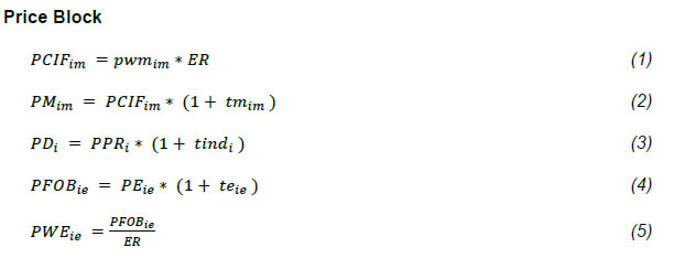 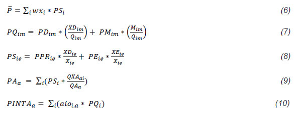 The above equations refer to different prices of the model. The Equation (1) represents prices of imported goods including cost, insurance and freight (PCIF) which is exogenously determined as world price (PWM) times the exchange rate (ER). The PCIF is inflated by the import tariff (tm) to get the import price (PM) as shown in Equation (2). The domestic price (PD) is determined by the producer’s price (PPR) and the indirect taxes (tind) as given in Equation (3). The Equation (4) refers to export price free on board (PFOB) is determined by producer’s price on export goods and export tax/subsidy (te). Then the world export prices are determined as PFOB divided by exchange rate (Equation 5). P̅ is the weighted average of the sales price which is taken as the numeraire in the model (Equation 6). The composite price (PQ) prevailing in the domestic market is the weighted sum of the domestic price (PD) and the import price (PM) as given in Equation (7). Similarly, Equation (8) gives the sales price (PS) received by the producer is a weighted sum of domestic sales price (PD) and export price (PE). The price of each activity output (PA) is defined as the weighted average of sales price (Equation 9). Price of intermediate demand (PINTA) for each activity output is the sum total of value of the intermediate input demand (aio) for that commodity as given in Equation 10. 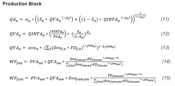 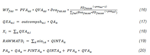 Domestic activity outputs (QA) are determined through the nested production functions. The first level of nesting determines aggregate intermediate demand (QINTA) and total value added (QVA) for each sector through the constant elasticity of substitution (CES) production function as shown in Equation 11. In the second level of nesting, intermediate demand for each sector (QINTA) is decided through Leontief coefficients (aio) of input-output table which was embedded in the SAM. The multiple of intermediate demand for each sector and the Leontief coefficient of the particular commodity to the specific sector gives commodity wise raw material demand from the particular sector. The sum total of commodity wise raw material demands from all sectors gives total raw material demand for respective commodities (Equation 19). Optimal factor demand (FD) for each labour and capital is determined through the CES production functions as shown in Equations 12 and 13. Here multiple labour types are defined on the basis of their education level and each labour is assumed to be mobile across all sectors. Capital is defined for broad sectors viz. agriculture, industry and services. As capital is assumed to be mobile within broad categories and immobile across these categories, we define three separate factor demand Equations 14, 15 and 16 for agriculture, industry and services respectively. These equations shows, factor price (WF) depends on total value added (QVA), price of value added (PVA) of each activity and respective factor demand (FD). Equations 17 shows that the output of each commodity produced by an activity is determined through fixed shares and the national total output of each commodity is simply the sum of output of that commodity produced by each activity (Equation 18). Equation 20 shows that value of each activity is equal to the sum of value of intermediate inputs and total value added for the particular sector. 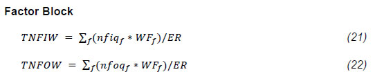 In Equation 21, total factor inflow from the world (TNFIW) at world price depends on the net factor inflow (nfiq), factor prices and exchange rate (ER). Similarly, total factor outflow from the world (TNFOW) at world price depends on the net factor outflow (nfoq), factor prices and exchange rate (ER) as shown in Equation 22. 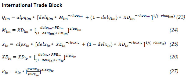 Here we assume that the traded goods are close but not perfectly substitutes with domestically produced goods, which is known as the Armington’s assumption. Total demand of each good (Q) is defined as a CES aggregation of domestically produced goods (XD) and imports (M) (Equation 23). The ratio of domestic goods and import is obtained as a function of domestic price (PD) and import price (PM) (Equation 24). Similarly, total output produced (X) is specified as the constant elasticity of transformation function of domestic demand (XD) and exports (E) (Equation 25). Ratio of domestic supply and exports depends on the ratio of export prices and domestic prices (Equation 26). The global demand for exports of a commodity is determined as a function of an exogenously fixed benchmark/ reference world market price (pwex) and endogenously determined export price (PWE) as given through Equation 27. Thus, here we the model is based on the small country assumption where the country cannot influence world prices. 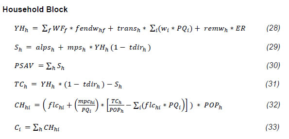 Total factor income is allocated to households by their income class. Here households are divided in 12 income classes based on their per capita consumption expenditure in rural and urban areas. Factor income of each income class depends on initial factor endowment (fendw) of those households. In addition, household income (YH) depends on total transfer income from government (trans) and remittances (remw) from abroad (Equation 28). Income (YH) net of direct taxes (tdir) is used to calculate disposable income of each income class. Then total disposable income is dived into private consumption (TC) and savings (S) on the basis of average and marginal propensity to save as shown in Equations 29 and 31. Total private savings over all households is simply the sum of savings of individual households (Equation 30). Sectoral private consumption (CH) is determined by linear expenditure system (LES) with underlying Stone-Geary type of loglinear utility functions in Equation 32. Finally, the total household demand for a commodity is arrived by summing over all households (Equation 33). The parameter values of the LES are calibrated to reproduce the consumption levels in the SAM. The consumer price index is calculated as a weighted average of composite sectoral prices and total consumption of each commodity to compute real income of each income class. 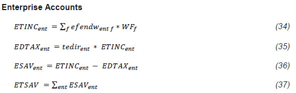
Enterprises are divided into two broad categories, viz. private and public enterprises. Total income of each enterprise (ETINC) is determined through total factor endowment (efendw) of those enterprises and factor prices (WF) (Equation 34). They pay direct taxes (EDTAX) depending on direct tax rate (tedir) (Equation 35) and save (ESAV) rest of their income (Equation 36). Total savings by enterprises is then the sum of the savings by private and public enterprises (Equation 37).
 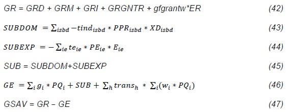 This section is related to government income and expenditure account. Total government revenue from direct taxes (GRD) includes direct tax payments by households and enterprises (Equation 38). Import tariff (GRM) is calculated by tariff rates and rupee value of total imports (Equation 39). Then government revenue from indirect taxes (GRI) is determined by indirect tax rates and value of domestic goods at producer’s price (Equation 40). Non-tax revenue (GRGNTR) is the total income from factor endowment owned by government (Equation 41). Thus total government revenue (GR) is the sum of direct tax, indirect tax (GRI), import tariff (GRM) and non-tax revenue (GRGNTR) (Equation 42). Total government expenditure (GE) consists of government consumption, subsidies (SUB) and transfer payment to households (Equation 46). Government provides subsidy to both domestic (SUBDOM) and export goods (SUBEXP) as shown in Equation 43 and 44 respectively. Government savings is calculated as the difference between government revenue and expenditure (Equation 47).  Total savings of the economy consists of household savings (PSAV), enterprise savings, government savings and rupee value of the foreign savings (Equation 48) whereas total investment (TINV) is divided into gross fixed capital formation (TGFCF) and total value of stock (TSTKV) (Equation 51). The total value of stocks is the sum of the value of stocks of individual commodities (Equation 49). Sectoral investment demand (Z) is determined from total fixed capital deflated by sectoral prices (PQ) (Equation 50). 
This segment explains all market clearing conditions to determine prices of each sector. The product market equilibrium condition is given in terms of total composite supply of each commodity and total demand of that good. Here total demand (Q) is determined by intermediate demand (RAWMATD), private consumption (C), government consumption (g) and investment demand (Z) (Equation 52). Total supply of the commodity is the sum of domestic production, imports less exports. The product prices change to equilibrate the product market. Here we assumed that exchange rate is fixed over the period. Thus supply and demand balance for foreign exchange market is determined by variation in foreign savings (FSAVW) in Equation 55. Export price changes to equilibrate the demand and supply of exports (Equation 53). Total supply of each factor depends on the factor endowment of households (fendw), enterprises (efendw), government (gfendw) and net foreign inflow of the factor (nfiq – nfoq) which are exogenously given in the model. But total demand of each factor is endogenously determined in the model and factor prices are determined by equilibrating total factor demand and supply (Equation 54). Then total investment (TINV) is determined by total savings of the economy as the model is specified in the default case as a Neo-Classical savings driven model (Equation 56).
Appendix 3: Additional results | Appendix Table 1: GDP multipliers | | | 2016-17 | 2017-18 | 2018-19 | 2019-20 | 2020-21 | 2021-22 | 2022-23 | 2023-24 | 2024-25 | 2025-26 | | I) With respect to Government consumption expenditure | | Set-A simulations | | | | | | | | | | | | RUN-01 | 0.04 | -0.14 | -0.34 | -0.54 | -0.75 | -1.00 | -1.28 | -1.63 | -1.98 | -2.36 | | RUN-02 | 0.69 | 0.68 | 0.67 | 0.67 | 0.66 | 0.66 | 0.67 | 0.67 | 0.67 | 0.68 | | RUN-03 | 0.05 | -0.18 | -0.45 | -0.77 | -1.16 | -1.62 | -2.17 | -2.94 | -3.86 | -4.98 | | RUN-04 | 0.63 | 0.62 | 0.62 | 0.61 | 0.61 | 0.61 | 0.62 | 0.63 | 0.64 | 0.65 | | Set-B simulations | | | | | | | | | | | | RUN-05 | 0.63 | 0.62 | 0.62 | 0.61 | 0.61 | 0.62 | 0.62 | 0.63 | 0.64 | 0.65 | | RUN-06 | 0.62 | 0.62 | 0.61 | 0.61 | 0.61 | 0.61 | 0.62 | 0.63 | 0.64 | 0.64 | | RUN-07 | 0.62 | 0.61 | 0.61 | 0.61 | 0.61 | 0.61 | 0.62 | 0.63 | 0.63 | 0.64 | | RUN-08 | 0.62 | 0.61 | 0.61 | 0.61 | 0.61 | 0.61 | 0.62 | 0.63 | 0.63 | 0.64 | | Set-C simulations | | | | | | | | | | | | RUN-09 | 0.73 | 0.73 | 0.74 | 0.75 | 0.76 | 0.77 | 0.81 | 0.83 | 0.85 | 0.88 | | RUN-10 | 0.72 | 0.71 | 0.70 | 0.69 | 0.69 | 0.69 | 0.70 | 0.70 | 0.71 | 0.72 | | II) With respect to government transfer expenditure to households | | Set-D simulations | | | | | | | | | | | | RUN-11 | 0.23 | 0.21 | 0.19 | 0.18 | 0.17 | 0.16 | 0.15 | 0.15 | 0.14 | 0.13 | | RUN-12 | 0.24 | 0.20 | 0.18 | 0.17 | 0.15 | 0.14 | 0.13 | 0.12 | 0.11 | 0.10 | | III) With respect to government investment expenditure | | Set-E simulations | | | | | | | | | | | | RUN-13 | -0.63 | -0.56 | -0.52 | -0.49 | -0.47 | -0.45 | -0.43 | -0.41 | -0.39 | -0.37 | | RUN-14 | -0.72 | -0.64 | -0.59 | -0.56 | -0.52 | -0.49 | -0.47 | -0.45 | -0.42 | -0.39 | | RUN-15 | -1.27 | -1.22 | -1.20 | -1.19 | -1.19 | -1.19 | -1.21 | -1.22 | -1.23 | -1.25 | | RUN-16 | 1.63 | 1.61 | 1.60 | 1.57 | 1.51 | 1.46 | 1.39 | 1.35 | 1.32 | 1.28 | Source: Authors’ calculations
 |
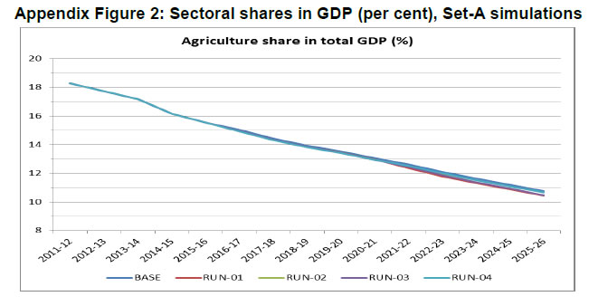 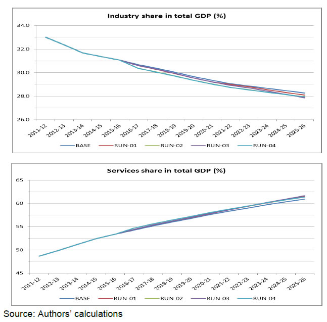 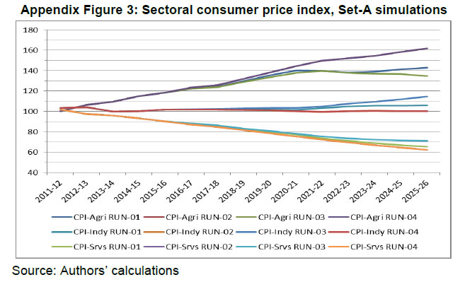
Glossary | Sets | | i | Commodity | | a | Activity | | f | Factors | | h | Households | | ent | Enterprises | | t | Time periods | | ia | Agricultural commodity | | ina | Non-agricultural commodity | | imm | Industrial commodity | | isrv | Services commodity | | isbd | Subsidised commodities | | itxd | Taxed commodities | | ie | Exportable | | iea | Agricultural exportable | | iei | Industrial exportable | | ies | Services exportable | | ine | Non-exportable | | im | Importable | | ima | Agricultural importable | | imi | Industrial importable | | ims | Services importable | | inm | Non-importable | | Endogenous Variables | | ER | Exchange rate Rupees per Dollar | | 𝑃𝐶𝐼𝐹𝑖𝑚 | Rupees import price cif | | 𝑃𝑀𝑖𝑚 | Rupees import price tariff inclusive | | 𝑃𝐸𝑖𝑒 | Rupees producer price on exportable | | 𝑃𝐹𝑂𝐵𝑖𝑒 | Rupees export price fob inclusive of export tax | | 𝑃𝑊𝐸𝑖𝑒 | Dollar export price fob | | 𝑃𝑃𝑅𝑖 | Producer price on domestic sales | | 𝑃𝐷𝑖 | Price of domestic good paid by domestic users | | 𝑃𝑄𝑖𝑚 | Price of composite good paid by domestic users | | 𝑃𝑆𝑖𝑒 | Sales price received by producers net of domestic and export taxes | | 𝑃𝐴𝑎 | Price of activity output | | 𝑃𝐼𝑁𝑇𝐴𝑎 | Price of activity - aggregate intermediates | | 𝑃𝑉𝐴𝑎 | Price of national activity - aggregate value added | | 𝑃̅ | Price index of domestic goods in domestic market | | 𝑊𝐹𝑓 | Price of factors | | 𝑀𝑖𝑚 | Imports | | 𝐸𝑖𝑒 | Export demand | | 𝑋𝐸𝑖𝑒 | Exports supply | | 𝑋𝐷𝑖𝑒 | Domestic demand from domestic production | | 𝑋𝑖 | Commodity output | | 𝑄𝑖𝑚 | Total demand for composite good national | | 𝑄𝐴𝑎 | Activity output | | 𝑄𝐼𝑁𝑇𝐴𝑎 | Activity aggregate intermediates | | 𝑄𝑉𝐴𝑎 | Activity value added | | 𝑄𝑋𝐴𝑎,𝑖 | Commodity output produced by activity | | 𝑅𝐴𝑊𝑀𝐴𝑇𝐷𝑖 | Raw materials (intermediate) demand | | 𝐶𝐻ℎ𝑖 | Household commodity demands by MPCE-deciles for Rural and Urban | | 𝐶𝑖 | Household commodity demand national | | 𝐹𝐷𝑓𝑎 | Factor demand in activities national | | 𝑡𝑑𝑖𝑟ℎ | Direct tax rate by MPCE-deciles for Rural and Urban | | 𝑌𝐻ℎ | Household total income | | 𝑇𝐶ℎ | Household consumption expenditure budget | | 𝐸𝑇𝐼𝑁𝐶𝑒𝑛𝑡 | Enterprise total income | | 𝐸𝐷𝑇𝐴𝑋𝑒𝑛𝑡 | Enterprise direct tax payment | | 𝐸𝑆𝐴𝑉𝑒𝑛𝑡 | Enterprise savings | | SAVCLSR | Savings closure adjustment | | TNFIW | Total Dollar net factor income from abroad | | TNFOW | Total Dollar net factor income to abroad | | 𝑍𝑖 | Fixed investment demand | | 𝑆ℎ | Household savings | | GRD | Government revenue from direct taxes | | GRM | Government revenue from import tariffs | | GRI | Government revenue from domestic indirect taxes | | GRGNTR | Government revenue from non-tax sources | | GR | Government revenue total | | SUBDOM | Government subsidies on domestic consumption | | SUBEXP | Government subsidies on exports | | SUB | Government subsidies total | | GE | Government expenditure total | | PSAV | Household savings total | | ETSAV | Enterprise savings total | | GSAV | Government savings | | TSAV | Total savings | | FSAVW | Dollar foreign savings | | TSTKV | Total value of changes in stocks | | TGFCF | Total value of gross fixed capital formation | | TINV | Total investment | | TGOLD | Total investment on gold | | 𝑉𝑇𝑋𝑖 | Implicit tax rate on commodities with administered prices | | 𝑖𝑚𝑟𝑡 | Infant mortality rate | | 𝑖𝑚𝑟ℎℎℎ𝑡 | Infant Mortality Rate by income classes | | 𝑑𝑜𝑟𝑡 | Dropout rate | | 𝑤𝑎𝑡𝑒𝑟𝑖𝑡 | Percentage of households with access to safe drinking water | | 𝑠𝑎𝑛𝑖𝑡𝑎𝑡𝑖𝑜𝑛𝑖𝑡 | Percentage of households with access to sanitation facilities | | 𝑝𝑦𝑖𝑙𝑟𝑡 | Percentage increase in Literacy rate | | 𝑝𝑦𝑖ℎ𝑒𝑝𝑡 | Percentage increase in percentage of adults completed higher education | | 𝑝𝑦𝑖𝑎𝑦𝑠𝑡 | Percentage increase in average years of schooling | | 𝑙𝑟𝑡 | Literacy rate | | Exogenous variables | | 𝑖𝑠ℎ𝑝𝑣𝑡𝑒𝑛𝑡𝑡 | Initial investment share of private enterprises | | 𝑖𝑠ℎ𝑝𝑢𝑏𝑒𝑛𝑡𝑡 | Initial investment share of public enterprises | | 𝑖𝑠ℎ𝑔𝑜𝑣𝑡𝑡 | Initial investment share of Government | | 𝑖𝑝𝑎𝑑𝑗𝑡 | Initial Partial adjustment factor for investments by capital types | | 𝑔𝑒ℎ𝑒𝑝𝑡 | Percentage of government expenditure in higher education | | 𝑝𝑦𝑖𝑝𝑐𝑔𝑒𝑒𝑡 | Per year increase in per capita government expenditure in education | | 𝑝𝑦𝑖ℎ𝑖𝑛𝑑𝑢𝑝𝑡 | Per year increase in the percentage of Hindu population | | 𝑝𝑦𝑖𝑠𝑡𝑡 | Per year increase in the percentage of ST population | | 𝑝𝑦𝑖𝑠𝑟𝑡 | Per year increase in sex ratio | | 𝑝𝑦𝑖𝑑𝑟𝑡 | Per year increase in dependency ratio | | 𝑝𝑦𝑖ℎℎ𝑖𝑙𝑟𝑝𝑡 | Per year increase in percentage of irrigated land-owners in rural area | | 𝑝𝑦𝑖𝑛𝑠𝑐𝑝𝑎𝑡 | Per year increase in no of higher or secondary schools or colleges per | | 𝑙𝑜𝑔𝑝𝑐𝑒𝑠𝑛𝑝𝑡 | Log per capita real public expenditure on SNP | | 𝑙𝑜𝑔𝑝𝑐𝑔𝑑𝑝𝑡 | Log per capita GDP | | 𝑙𝑜𝑔𝑝𝑐𝑔𝑑𝑝ℎℎ𝑡 | Log per capita GDP by income classes | | 𝑝𝑐𝑔𝑑𝑝𝑡 | Per capita GDP | | 𝑝𝑐𝑔𝑑𝑝ℎℎ𝑡 | Per capita GDP by income classes | | 𝑢𝑟𝑏𝑡 | Urbanisation | | 𝑝𝑐𝑟𝑒𝑒𝑒𝑡 | Per capita real public expenditure on elementary education | | 𝑙𝑜𝑔𝑝𝑐𝑟𝑒𝑒𝑒𝑡 | Log per capita real public expenditure on elementary education | | 𝑙𝑜𝑔𝑝𝑐𝑟𝑒𝑤𝑠𝑖𝑡 | Log per capita real public expenditure on water and sanitation | | gfgrantw | Dollar foreign grant received by Government | | 𝑝𝑤𝑚𝑖 | Dollar world price imports | | 𝑝𝑤𝑒𝑥𝑖 | Dollar reservation world price exports | | 𝑡𝑚𝑖 | Import tariff | | 𝑡𝑒𝑖 | Export tax | | 𝑡𝑖𝑛𝑑𝑖 | Indirect tax rate on domestic sales | | 𝑡𝑑𝑖𝑟ℎ | Direct tax rate on households | | 𝑡𝑒𝑑𝑖𝑟𝑒𝑛𝑡 | Direct tax rate on enterprises | | 𝑎𝑖𝑜𝑖𝑎 | Input-output coefficient for activity | | 𝑜𝑢𝑡𝑐𝑜𝑚𝑝𝑠ℎ𝑎𝑖 | Commodity output composition activity | | 𝑎𝑣𝑎𝑠ℎ𝑎 | Value added share in activity output | | ℎ𝑠ℎ𝑎𝑐ℎ | Household share in endowment of all capital types | | ℎ𝑠ℎ𝑠𝑟𝑣𝑘ℎ | Household share in endowment of services capital | | 𝑎𝑙𝑓𝑞𝑎𝑎 | CES scale - National activity - output nest level-1 | | 𝑑𝑙𝑓𝑞𝑎𝑎 | CES share - National activity - output nest level-1 | | 𝑟ℎ𝑜𝑞𝑎𝑎 | CES rho - National activity - output nest level-1 | | 𝑠𝑖𝑔𝑞𝑎𝑎 | CES elasticity - National activity - output nest level-1 | | 𝑎𝑙𝑓𝑞𝑣𝑎𝑎 | CES scale - National activity - value added | | 𝑑𝑙𝑡𝑞𝑣𝑎𝑓𝑎 | CES share - National activity - value added | | 𝑟ℎ𝑜𝑞𝑣𝑎𝑎 | CES rho - National activity - value added | | 𝑠𝑖𝑔𝑞𝑣𝑎𝑎 | CES elasticity - National activity - value added | | 𝑎𝑙𝑝𝑞𝑖 | Armington imports scale | | 𝑑𝑒𝑙𝑞𝑖 | Armington imports share | | 𝑟ℎ𝑜𝑞𝑖 | Armington imports rho | | 𝑠𝑖𝑔𝑞𝑖 | Armington imports elasticity | | 𝑎𝑙𝑝𝑥𝑖 | CET exports scale | | 𝑑𝑒𝑙𝑥𝑖 | CET exports share | | 𝑟ℎ𝑜𝑥𝑖 | CET exports rho | | 𝑠𝑖𝑔𝑥𝑖 | CET exports elasticity | | 𝑒𝑥𝑏𝑎𝑟𝑖 | Base export quantities in export demand equation | | 𝑒𝑙𝑒𝑥𝑝𝑖 | Elasticity in export demand equation | | 𝑓𝑒𝑛𝑑𝑤ℎ𝑓 | Factor endowments households | | 𝑒𝑓𝑒𝑛𝑑𝑤𝑒𝑛𝑡𝑓 | Factor endowments enterprises | | 𝑔𝑓𝑒𝑛𝑑𝑤𝑓 | Factor endowments government | | 𝑠𝑦ℎ𝑓 | Share household in total factor income | | 𝑛𝑓𝑖𝑤𝑓 | Dollar net factor income from abroad | | 𝑛𝑓𝑜𝑤𝑓 | Dollar net factor income outflow to abroad | | 𝑡𝑟𝑎𝑛𝑠ℎ | Government transfers to households | | 𝑟𝑒𝑚𝑤ℎ | Dollar remittances received by households | | 𝑛𝑓𝑖𝑞𝑓 | Net factor exports | | 𝑛𝑓𝑜𝑞𝑓 | Net factor imports | | 𝑓𝑟𝑖𝑠𝑐ℎℎ | Household Frisch parameter | | 𝑎𝑙𝑝𝑠ℎ | Constant term in household savings function | | 𝑚𝑝𝑠ℎ | Marginal propensity to save term in household savings function | | 𝑓𝑙𝑐ℎ 𝑖 | LES floor consumption | | 𝑚𝑝𝑐ℎ 𝑖 | LES marginal propensity to consume | | 𝑎𝑝𝑐ℎ 𝑖 | Average propensity to consume - used to calibrate LES parameters | | 𝑔𝑖 | Government consumption | | 𝑐𝑠𝑡𝑘𝑞𝑖 | Changes in stock quantities | | 𝑤𝑥𝑖 | Output weight | | 𝑤𝑞𝑖 | Composite expenditure weight | | 𝑤𝑧𝑖 | Investment weight | | 𝑤𝑚𝑖𝑚 | Import weight | | 𝑝𝑜𝑝𝑙𝑛ℎ | Population in each household decile | |