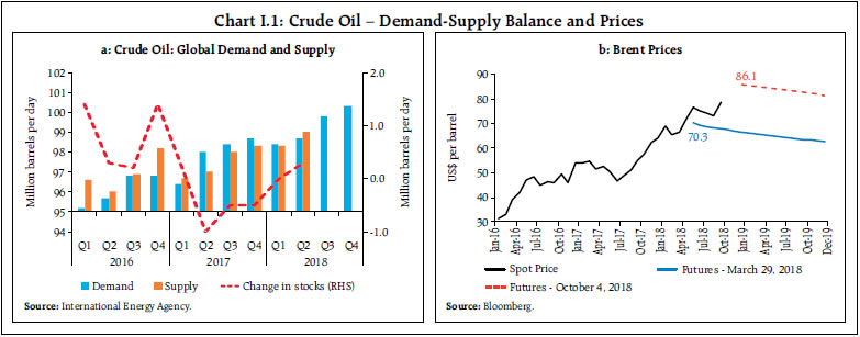
| I. Macroeconomic Outlook While domestic activity has continued to exhibit resilience and stability after the April 2018 Monetary Policy Report, the external environment has remained challenging and imparted downside risk to India’s growth prospects. The soft headline inflation readings for July and August 2018 relative to projections imply a largely benign food prices outlook in the near term even as upside risks to inflation over the 12-month ahead horizon appear to be rising modestly due to global financial market volatility and surging oil prices. I.1 Key Developments since April 2018 MPR In the period following the Monetary Policy Report (MPR) of April 2018, several risks it had flagged have been materialising on an ongoing basis. The global macroeconomic and financial environment has been roiled by bouts of financial market volatility, retaliatory trade protectionism among major economies of the world, elevated and volatile crude oil prices, and recurring jitters around the efficacy of managing monetary policy normalisation in the US amidst a late-in-the-cycle US fiscal stimulus, occurring all at once, lashing emerging market economies (EMEs) as an asset class with asset price shocks and capital outflows. More recently, vulnerabilities surfacing amongst specific EMEs have produced powerful contagion effects. Taken together, these global factors appear to be increasing risks around India’s growth prospects over the next 12-month horizon with a slant to the downside. Global growth itself is getting differentiated across economies and the cyclical upswing in global trade that had started in Q4:2017 is being stifled by rising trade tensions. Meanwhile, domestic economic activity has continued to exhibit resilience and stability in these highly unsettled global conditions. On the agricultural front, the spatial distribution of south-west monsoon was somewhat skewed, although most of the kharif crop growing states received normal rainfall. Industrial activity has gathered pace and the outlook for the services sector is gradually improving. Inward foreign direct investment remains buoyant. The slow firming up of private consumption and investment are expected to be sustained in H2:2018-19. The soft headline inflation readings for July and August 2018 relative to projections imply a largely benign food prices outlook in the near term; however, volatility in global financial markets and surging oil prices remain upside risks to inflation over the 12-month ahead horizon. These developments pose challenges for the setting of monetary policy in India. Monetary Policy Committee: April-August 2018 During April-August 2018, the Monetary Policy Committee (MPC) met thrice in accordance with its bi-monthly schedule. Maintaining status quo in its April 2018 meeting, the MPC increased the policy repo rate by 25 basis points (bps) successively in its June and August 2018 meetings. In its June 2018 meeting, the MPC’s vote was unanimous against the backdrop of rising inflation, upward revision in inflation projections, sharper than anticipated increase in crude oil prices, and hardening of households’ inflation expectations. In August, however, the MPC’s vote was by a majority of 5:1. The decision by majority was influenced by further hardening of inflation and inflation expectations amidst uncertainty around the impact of the minimum support price (MSP) hikes. The MPC’s voting pattern, which reflects differences in individual members’ assessments and expectations as well as relative weights on policy goals, is also observed in other central banks (Table I.1). Macroeconomic Outlook Chapters II and III analyse developments relating to prices and costs and demand and supply conditions during the first half of 2018-19, comparing outcomes versus forecasts and setting reasons underlying divergences. Turning to the outlook, developments in key macroeconomic variables over the past six months warrant revisions in the baseline assumptions (Table I.2). | Table I.1 Monetary Policy Committees and Voting Patterns | | Country | Policy Meetings: April - September 2018 | | Total Meetings | Meetings With Full Consensus | Meetings With Dissents | | Brazil | 4 | 4 | 0 | | Chile | 4 | 4 | 0 | | Colombia | 4 | 4 | 0 | | Czech Republic | 4 | 2 | 2 | | Hungary | 6 | 6 | 0 | | Israel | 4 | 0 | 4 | | Japan | 4 | 0 | 4 | | South Africa | 3 | 2 | 1 | | Sweden | 3 | 0 | 3 | | Thailand | 4 | 1 | 3 | | UK | 4 | 2 | 2 | | US | 4 | 4 | 0 | | Sources: Central bank websites; and Bloomberg. | First, international crude oil prices have firmed up by more than US$ 15 per barrel over the April 2018 MPR baseline assumption. Given the current demand-supply assessment and signals extracted from the futures market, the baseline scenario assumes crude oil prices (Indian basket) to average US$ 80 a barrel in the second half of 2018-19 (Chart I.1). Second, the exchange rate of the Indian rupee (INR) visà- vis the US dollar has depreciated from its end-March level, reflecting (i) the general strengthening of the US dollar across major currencies; (ii) higher crude oil prices widening the trade and current account deficits; (iii) portfolio outflows; and (iv) risk aversion among portfolio investors towards EMEs after the country-specific developments in Turkey and Argentina. As on October 4, the INR had depreciated by 11.8 per cent against the US dollar from its level at end-March 2018. | Table I.2: Baseline Assumptions for Near-Term Projections | | Indicator | April 2018 MPR | Current (October 2018) MPR | | Crude Oil (Indian Basket) | US$ 68 per barrel | US$ 80 per barrel during H2:2018-19 | | Exchange rate | ₹65.5/US$ | ₹72.5/US$ | | Monsoon | Normal for 2018 | 9 per cent below long period average | | Global growth | 3.9 per cent in 2018 | 3.9 per cent in 2018 | | 3.9 per cent in 2019 | 3.9 per cent in 2019 | | Fiscal deficit (per cent of GDP) | To remain within BE 2018-19
Centre: 3.3
Combined (Centre and States): 6.0 | To remain within BE 2018-19
Centre: 3.3
Combined (Centre and States): 5.9 | | Domestic macroeconomic/ structural policies during the forecast period | No major change | No major change | Notes: 1. The Indian basket of crude oil represents a derived numeraire comprising sour grade (Oman and Dubai average) and sweet grade (Brent) crude oil.
2. The exchange rate path assumed here is for the purpose of generating staff’s baseline growth and inflation projections and does not indicate any ‘view’ on the level of the exchange rate. The Reserve Bank is guided by the objective of containing excess volatility in the foreign exchange market and not by any specific level of and/or band around the exchange rate.
3. Global growth projections are from the World Economic Outlook (January 2018 and July 2018 Updates), International Monetary Fund (IMF).
4. BE: Budget estimates. |
 Third, global economic activity has expanded, broadly in line with the baseline projections given by the International Monetary Fund (IMF) in April (Chart I.2). However, it has become uneven and less synchronised across regions. Uncertainty has heightened on account of escalating protectionism and tariff wars, tightening of global financial conditions, and higher oil prices, all posing downside risks to global growth. The recovery in world trade is losing momentum.1 Finally, the south-west monsoon rainfall (June- September 2018) was 9 per cent below long period average, vis-à-vis the baseline assumption of normal monsoon made in April. I.2 The Outlook for Inflation Headline consumer price index (CPI) inflation averaged 4.4 per cent during 2018-19 up to August [4.1 per cent, excluding the estimated impact of house rent allowances (HRAs) for central government employees]. A broad-based uptick in inflation in respect of prices of fuel, transportation, personal care/effects, education and health services was largely offset by the unexpectedly and unseasonally benign food inflation (Chapter II). Looking ahead, it is useful to read into the signals emitted by inflation expectations of firms and households. By shaping price and wage setting behaviour, they influence future inflation. Inflation expectations also adapt to actual inflation outcomes of salient items such as food and fuel. Inflation expectations of urban households surveyed by the Reserve Bank exhibited a mixed picture in its September 2018 round2: they increased by 50 bps over the previous round for the three months ahead horizon and softened by 30 bps for the one year ahead horizon. The proportion of respondents expecting the general price level to increase by more than the current rate, however, declined marginally in the September round for the three months ahead horizon and was almost unchanged for the one year ahead horizon (Chart I.3). Manufacturing firms polled in the July-September 2018 round of the Reserve Bank’s industrial outlook survey expected higher cost of raw materials in Q3:2018-19 (Chart I.4).3 Consequently, respondents anticipated input prices to firm up further and muted profit margins in spite of higher selling prices. According to the Nikkei’s purchasing managers’ survey, firms in both the manufacturing and services sectors raised output prices in September 2018 in the face of input cost pressures. Professional forecasters surveyed by the Reserve Bank in September 2018 expected CPI inflation to fall from 4.8 per cent in Q1:2018-19 to 4.1 per cent in Q3 and then pick up to 5.1 per cent by Q2:2019-20 (Chart I.5).4 Taking into account the initial conditions, signals from forward-looking surveys and estimates from structural and other models5, CPI inflation is projected to pick up from 3.7 per cent in August 2018 to 3.9 per cent in Q3:2018-19 and 4.5 per cent in Q4:2018-19, with risks somewhat tilted to the upside (Chart I.6). The projected increase in inflation from current levels reflects the waning away of favourable base effects and anticipates the feeding through of the impact of the increase in MSPs into retail inflation. The direct impact of the increase in HRA by central government has started waning and will fade away completely by December 2018. Excluding the estimated impact of HRA for central government employees, CPI inflation is projected at 3.8 per cent in Q3:2018-19 and 4.5 per cent in Q4:2018-19. The 50 per cent and the 70 per cent confidence intervals for headline inflation in Q4:2018-19 are 3.6-5.7 per cent and 3.1-6.4 per cent, respectively.  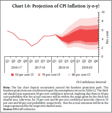 For 2019-20, structural model estimates indicate that inflation will move in a range of 4.5-4.8 per cent, assuming a normal monsoon and no major exogenous/ policy shocks. The 50 per cent and the 70 per cent confidence intervals for Q4:2019-20 are 3.4-6.3 per cent and 2.7-7.2 per cent, respectively. There are upside and downside risks to the baseline inflation path. As stated earlier, the announced increase in MSPs for kharif crops has been much bigger than in the recent past, but there is considerable uncertainty about the exact impact of the scale and timing of government procurement operations. Other upside risks in the context of the baseline projection include supply disruptions in the global crude oil market, volatility in international financial markets and second round effects of the staggered HRA revisions by state governments. A major downside risk to the baseline could be decline in demand for oil due to global growth slowdown on account of rising trade tensions, which may help bring down oil prices. I.3 The Outlook for Growth The April 2018 MPR had projected an acceleration in real gross domestic product (GDP) growth in 2018-19 on the back of: (a) the goods and services tax (GST) stabilising; (b) improving credit offtake; (c) likely boost to investment from primary market resource mobilisation; (d) the process of recapitalisation of public sector banks and resolution of distressed assets under the Insolvency and Bankruptcy Code (IBC); (e) buoyant global trade; and (f) the thrust to the rural and infrastructure sectors in the Union Budget 2018- 19. Most of these have materialised, but to varying extent. However, global trade growth, as stated earlier, seems to be losing its synchronised momentum and this may hinder India’s export prospects. The uneven spatial distribution of the south-west monsoon is another factor that has also imparted some uncertainty to the agricultural outlook and inflation. Turning to forward-looking surveys, consumer confidence over the year ahead improved marginally in the September 2018 round of the Reserve Bank’s survey, reflecting an optimism on incomes and prices (Chart I.7).6 Optimism in the manufacturing sector for the quarter ahead improved in the September 2018 round of the Reserve Bank’s industrial outlook survey on account of higher order books and selling prices (Chart I.8).
| Table I.3: Business Expectations Surveys | | Item | NCAER Business Confidence Index (August 2018) | FICCI Overall Business Confidence Index (September 2018) | Dun and Bradstreet Composite Business Optimism Index (July 2018) | CII Business Confidence Index (September 2018) | | Current level of the index | 114.4 | 65.4 | 80.6 | 64.9 | | Index as per previous survey | 131.4 | 71.0 | 85.0 | 60.1 | | % change (q-o-q) sequential | -12.9 | -7.9 | -5.2 | 8.0 | | % change (y-o-y) | -15.9 | -1.1 | 11.7 | 11.3 | Notes: 1. NCAER: National Council of Applied Economic Research.
2. FICCI: Federation of Indian Chambers of Commerce & Industry.
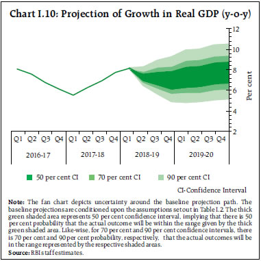
3. CII: Confederation of Indian Industry. | Surveys by other agencies indicate a mixed picture on future business expectations (Table I.3). Firms in the manufacturing and services sectors polled in the Nikkei’s purchasing managers’ surveys (September 2018) were optimistic about their output prospects a year ahead, driven by expected improvement in demand. In the September round of the Reserve Bank’s survey, professional forecasters expected real GDP growth to decelerate from 8.2 per cent in Q1:2018-19 to 6.9 per cent in Q4 and then recover to 7.4 per cent in Q2:2019- 20 (Chart I.9 and Table I.4). Taking into account the baseline assumptions, monetary policy tightening of 50 bps during June- August 2018, survey indicators and model forecasts, real GDP growth is projected to improve from 6.7 per cent in 2017-18 to 7.4 per cent in 2018-19 – 8.2 per cent in Q1, 7.4 per cent in Q2, 7.3 per cent in Q3 and 7.1 per cent in Q4 – with risks broadly balanced around this baseline path (Chart I.10). For 2019-20, structural model estimates indicate real GDP growth at 7.6 per cent, with quarterly growth rates in the range of 7.4-7.9 per cent, assuming a normal monsoon and no major exogenous or policy shocks. Strengthening investment activity and a further pick-up in credit growth impart an upside bias to the baseline growth projections. However, recent protectionist measures by major economies, threats of currency wars and the uncertainty associated with the pace of monetary policy normalisation in the US and other major advanced economies pose downside risks to the baseline growth path. 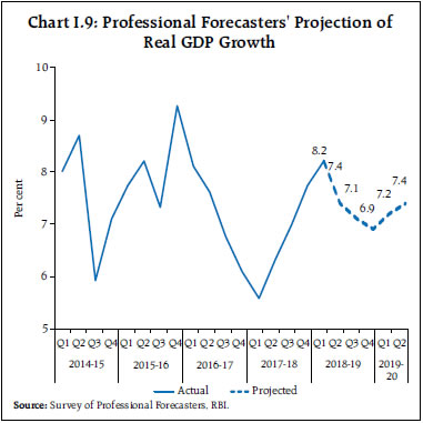
| Table I.4: Projections – Reserve Bank and Professional Forecasters | | (Per cent) | | | 2018-19 | 2019-20 | | Reserve Bank’s Baseline Projections | | | | Inflation, Q4 (y-o-y) | 4.5 | 4.6 | | Inflation excluding the estimated impact of HRA for central government employees, Q4 (y-o-y) | 4.5 | 4.6 | | Real GDP growth | 7.4 | 7.6 | | Median Projections of Professional Forecasters | | | | Inflation, Q4 (y-o-y) | 4.5 | 5.1# | | Real GDP growth | 7.4 | 7.5 | | Gross domestic saving (per cent of GNDI) | 29.8 | 30.0 | | Gross fixed capital formation (per cent of GDP) | 28.8 | 29.1 | | Credit growth of scheduled commercial banks | 12.0 | 12.3 | | Combined gross fiscal deficit (per cent of GDP) | 6.2 | 5.9 | | Central government gross fiscal deficit (per cent of GDP) | 3.3 | 3.1 | | Repo rate (end-period) | 7.00 | 7.00# | | Yield on 91-days treasury bills (end-period) | 7.2 | 7.2 | | Yield on 10-year central government securities (end-period) | 8.1 | 8.0 | | Overall balance of payments (US$ billion) | -20.7 | 0.3 | | Merchandise export growth | 10.4 | 9.7 | | Merchandise import growth | 14.3 | 8.4 | | Current account balance (per cent of GDP) | -2.7 | -2.5 | #: Forecast for Q2:2019-20; GNDI: Gross National Disposable Income.
Sources: RBI staff estimates; and Survey of Professional Forecasters (September 2018). |
 I.4 Balance of Risks The baseline projections of inflation and growth presented in the previous two sections are conditional on assumptions relating to key variables such as crude oil prices, external demand, exchange rate movements and fiscal stance (Table I.2) as well as the impact of higher MSPs. There are several uncertainties around the baseline assumptions, however, which could pose risks to baseline projections. The sensitivity of the baseline projections to plausible alternative scenarios is set out below. (i) International Crude Oil Prices Sharp swings in global crude prices over the past six months impart uncertainty to the outlook. The baseline scenario assumes crude oil prices (Indian basket) at US$ 80 per barrel in the second half of 2018-19. Upside risks to the baseline assumption can emanate from geo-political developments and supply disruptions. For a net energy importer like India, the dynamics of international crude price movements have significant macroeconomic implications. Box I.1 presents a scenario in which the Indian basket price increases by 10 per cent to US$ 88 per barrel, which is plausible under the current global crude oil price volatility. Under this scenario, inflation could increase by 20 bps and real GDP growth could be lower by around 15 bps in relation to their respective baselines given in Sections I.2 and I.3 (Charts I.11a and I.12a). Assuming that the Indian basket crude oil price increases by 20 per cent to US$ 96 a barrel, inflation and GDP growth could turn out to be 40 bps above and 30 bps below their respective baselines. Conversely, crude oil prices could soften below the baseline assumption if, for instance, there is a larger than expected shale gas supply and weaker than expected global demand due to growth slowing down on account of protectionist measures. As a result, if the price of the Indian basket of crude falls by 10 per cent to US$ 72 per barrel, inflation could ease by around 20 bps with a boost of 15 bps to growth. (ii) Global Growth In the baseline scenario, global growth is expected to be stronger in 2018 and 2019 relative to 2017. While the pace of global growth has been maintained in Q2:2018, it has turned uneven with new risks clouding the outlook. Escalating protectionism and rising geopolitical tensions could weigh on external demand. Tightening of financial conditions on the back of US monetary policy normalisation and expansionary US fiscal policy and uncertainty about the pace of further normalisation could also dampen global demand. If global growth slips by 50 bps, domestic growth and inflation could be around 20 bps and 10 bps below their respective baseline trajectories. However, if inflation remains benign in major advanced economies, a more gradual pace of monetary policy normalisation in these economies could boost global demand and global commodity prices. In this scenario, assuming that global growth surprises by 25 bps on the upside, domestic growth and inflation could edge higher by around 10 bps and 5 bps, respectively (Charts I.11a and I.12a). (iii) House Rent Allowances – Implementation by States Following the increase in pay and allowances by the central government for its employees based on the recommendations of the 7th central pay commission (CPC), some state governments have revised pay and allowances for their employees. If all state governments implement the increase in pay and allowances – especially HRAs – of an order similar to that of the central government, and if these get reflected in CPI, headline inflation could be around 100 bps above the baseline on account of the direct statistical effect on house rents (Chart I.11b). Additional indirect effects could also arise from higher demand and inflation expectations. As noted by the MPC in its recent resolutions, the direct statistical impact of HRA revisions will be looked through for policy purposes, while being watchful for any second-round effects. Box I.1: Macroeconomics of Crude Oil Prices Crude oil prices (Indian basket) increased from US$ 47 per barrel in June 2017 to US$ 78 in September 2018, an increase of 67 per cent in a span of 15 months. It is estimated that a US$ 10 increase in the price of international crude oil could reduce output in the OECD area by 20 bps after two years and raise inflation by 20 bps in the first year and by another 10 bps in the second year (OECD, 2011). For large net energy importers like India – 80 per cent of India’s crude oil requirement is met through imports – recent estimates suggest that real GDP growth could decline from its current trajectory, while inflation could rise significantly above target, rendering the current favourable macroeconomic conditions vulnerable. In addition, it is estimated that for every US$ 1 increase in the price of a barrel of crude, India’s current account deficit could widen by US$ 0.8 billion. Increases in crude oil prices impact economic activity through a variety of channels. Therefore, it is important to examine their effects in a general equilibrium context. The RBI’s workhorse Quarterly Projection Model (QPM) in its Forecasting and Policy Analysis System (FPAS), which draws its analytical underpinnings from new Keynesian foundations7, provides the flexibility to incorporate these various channels. There is the cost push channel that operates through the prices of non-administered fuel products i.e., petrol and diesel, whereby energy costs impact firms’ input costs, including transportation and other intermediate services. In addition, crude price increases are transmitted to the domestic economy through reduction in global demand, adverse price movements in respect of imports and exports, and undue volatility in the exchange rate. These diverse channels produce substitutions between energy and non-energy consumption, a reduction in output and an increase in inflation. The monetary policy response to these outcomes can, in turn, set off a chain of macroeconomic adjustments. The QPM depicts the various channels through which this transmission works (Chart I.1.1). A 10 per cent increase in international crude prices imparts a shock to petroleum product prices. Headline inflation goes up instantaneously by 13 bps, which takes up to a year to wear off. Furthermore, an increase in petroleum prices imparts cost push effects, which contribute about 15 bps to the increase in headline inflation. People react by spending less on non-oil items of consumption, reducing demand. To the extent that firms are not able to pass through the increase in oil prices to product prices, it reduces their profit margins, cash flows and investment. As a result, aggregate demand declines, leading to a negative contribution to inflation in the range of 5-10 bps. The crude oil price increase can also lead to a deterioration in the trade deficit, which can put downward pressure on the rupee, translating into an additional 10 bps increase in inflation. Consequently, monetary policy tightening is required to bring inflation back to target. The monetary policy reaction widens the output gap, compressing demand and thereby inflation. At its peak, the impact of the 10 per cent increase in crude oil price shock is expected to reduce growth by 15 bps and push up headline inflation by around 20 bps. 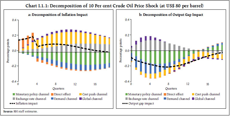 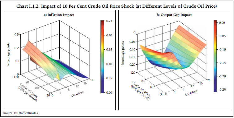 The effect of crude oil prices on domestic inflation and output depends upon not only on the extent of the change in crude oil prices but also on their initial level. This is because retail petroleum product prices contain several elements which are largely fixed – for example, excise duty and refining costs – while the base price moves in line with the movements in international crude oil prices and the exchange rate. The value added tax component moves in line with prices charged to dealers (inclusive of excise duty). The higher the level of crude oil prices, the smaller is the proportion of fixed elements and larger is the impact of a given increase in crude oil prices on domestic petrol and diesel inflation, and hence on overall inflation and output (Chart I.1.2). For instance, an increase of 10 per cent in crude oil prices from US$ 30 per barrel to US$ 33 per barrel is estimated to increase inflation by 13 bps, while a similar order of increase from US$ 100 a barrel to US$ 110 a barrel could pull up inflation by around 22 bps. References: Benes, Jaromir, et al. (2016), “Quarterly Projection Model for India: Key Elements and Properties”, RBI Working Paper Series, No. 08/2016. OECD (2011), “The Effects of Oil Price Hikes on Economic Activity and Inflation”, OECD Economics Department Policy Notes, No. 4. |
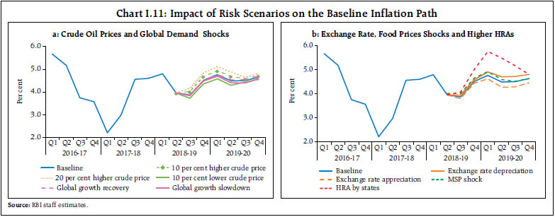 (iv) Exchange Rate The INR depreciated vis-à-vis the US dollar during April-September, reflecting both domestic and global developments. Looking ahead, a faster pace of monetary policy normalisation by the US Fed than currently factored in by financial markets, rising trade protectionism, threat of currency wars, and higher international crude oil prices are some of the factors that could exert downward pressure on the Indian rupee. Assuming a depreciation of the Indian rupee by around 5 per cent relative to the baseline, inflation could increase by around 20 bps, while the likely boost to net exports could push up growth by around 15 bps. On the other hand, India could also attract large inflows with its reasonably sound domestic fundamentals relative to its peers and the various initiatives taken by the government to boost investment. An appreciation of the Indian rupee by 5 per cent in this scenario could soften inflation by around 20 bps and GDP growth by around 15 bps in 2018-19 (Charts I.11b and I.12b). 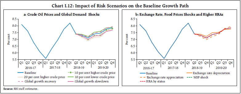 (v) Food Inflation The large increase in MSPs for kharif crops announced by the government in July 2018 can have a direct impact on food inflation and second round effects on headline inflation through relative price adjustments, higher demand on the back of higher rural incomes and increase in inflation expectations. The baseline projections incorporate the likely effect of the increase in MSPs on inflation, assuming normal procurement by the government in line with past trends (Box II.1). However, if procurement operations turn out to be larger than assumed, headline inflation could increase by around 20 bps above the baseline. (vi) Fiscal Slippage The baseline projections assume a fiscal stance as announced in the Union and State budgets for 2018-19. Higher MSPs combined with stepped-up food procurement operations and unbudgeted farm loan waivers by states pose upside risks to the fiscal outlook. Should there be fiscal slippage at the centre and/or state levels, it could result in greater market volatility, crowding out of private investment and higher inflation. Quantitative estimates of these risks will, however, be reliant on incoming data right up to the April 2019 MPR. I.5 Conclusion To sum up, real GDP growth is expected to accelerate in 2018-19 vis-à-vis 2017-18, with the pace of growth easing in H2 relative to H1. Stabilisation of the goods and services tax, progress on resolution of distressed assets under the insolvency and bankruptcy code and initiatives towards strengthening of bank balance sheets are supporting economic and investment activity. However, the uncertain global environment poses an important downside risk to the domestic growth outlook. Inflation is expected to pick up from its current levels as the MSPs for kharif crops feed into domestic food inflation and favourable base effects dissipate. Volatile crude oil prices and the volatility in international financial markets pose the primary upside risks to the inflation outlook. ________________________________________________________________________
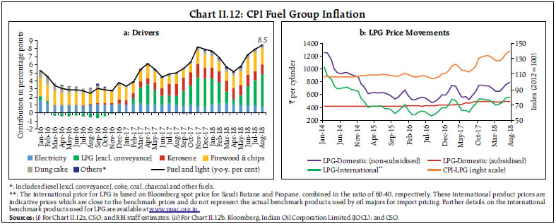
II. Prices and Costs Inflation has eased in Q2:2018-19 on an unusual ebbing in the momentum of food prices, after rising strongly in Q1 on the back of surging prices of non-food items (including the impact of 7th CPC’s HRA increase) across categories. Input costs rose sharply in Q1 and remained firm in Q2, largely due to increase in fuel prices. Wage pressures remained contained in both rural and organised sectors. Over the first half of 2018-19, the course of consumer price index (CPI) inflation has been shaped by diverse pulls. Within major groups, while food inflation remained soft in Q1:2018-19, and declined sharply in July and August 2018, fuel and light inflation rose noticeably, tracking international prices. Inflation in CPI excluding food and fuel also firmed up in Q1:2018-19 and remained elevated through July- August, notwithstanding some softening. The impact of the increase in house rent allowances (HRA) for central government employees on headline inflation has started to ebb from July.1 Adjusting for the HRA impact, headline inflation in August was estimated at 3.4 per cent as against the print of 3.7 per cent and inflation in CPI excluding food and fuel was estimated at 5.4 per cent against the reading of 6.0 percent (Chart II.1).2 The MPR of April 2018 had projected CPI inflation to increase from 4.6 per cent observed in Q4:2017-18 to 5.1 per cent in Q1:2018-19 and then moderate to 4.7 per cent in Q2. Excluding the estimated impact of HRA, CPI inflation was projected at 4.7 per cent in Q1 and then moderate to 4.4 per cent in Q2. Actual inflation outcomes have tracked these projections directionally; in terms of magnitude, however, inflation undershot projections by a considerable margin – 28 basis points (bps) in Q1 and 74 bps in Q2 up to August (Chart II.2) – entirely on account of a surprising persistence in the softening of prices of fruits, particularly in Q2, and lower than usual hardening in prices of vegetables in the summer months. Food inflation fell from 3.7 per cent in Q4:2017-18 to 3.1 per cent in Q1:2018-19. This is a significant development because it occurred on a base which reflected the after effects of demonetisation in depressing prices of fruits and vegetables in Q1 a year ago. Subsequently, food inflation plunged further to 1.3 per cent in July-August as strong favourable base effects coincided with inexplicable weak momentum of food prices. In fact, ebbing food inflation more than offset the impact of higher than projected crude oil prices – US$ 73.5 per barrel, on an average, during H1:2018-19 vis-à-vis the baseline assumption of US$ 68 per barrel in April 2018. 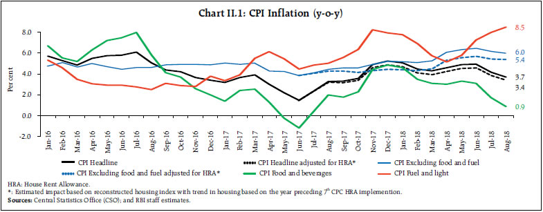 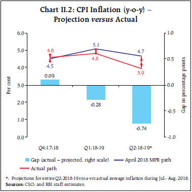 II.1 Consumer Prices As stated earlier, headline inflation dynamics in H1:2018-19 have reflected divergent movements among constituents which are revealed when momentum and base effects are disentangled. In the case of food items, there has been an unusually low momentum in prices of vegetables and an unexpected decline in prices of fruits in H1. In Q2, base effects turned favourable and along with unseasonally low momentum pulled down food inflation to just 1.3 per cent (up to August 2018) well below its quarterly trend level of six years (7.1 per cent). In the case of items excluding food and fuel, momentum in prices remained strong during April-May in Q1. Thereafter, in Q2 so far, momentum effects have been offset by favourable base effects. As a result, the monotonic hardening of headline inflation from 4.3 per cent in March 2018 to 4.9 per cent by June reversed and inflation fell to 3.7 per cent in August (Chart II.3). On an average, the distribution of inflation across CPI groups in 2018 so far had striking similarities with the outcomes in 2017, a period that also saw soft inflation readings coming from moderation in food inflation in the post-demonetisation period. Median inflation rates were in the range of 4.3-4.8 per cent in both the years and inflation exhibited considerable negative skew on account of deflation in pulses and sugar prices (Chart II.4). Diffusion indices of price changes in CPI items suggest that on a seasonally adjusted basis, a broadening swathe of goods and almost all services have experienced price increases since July, implying that soft headline inflation reading is occurring alongside generalised price increases across goods and services (Chart II.5).3 II.2 Drivers of Inflation A historical decomposition of inflation shows that large and sequential supply side shocks, emanating essentially from food group, have defined the overall change in headline inflation trajectory since Q3:2016- 17. In H1:2018-19, several factors impacted inflation – a favourable food supply shock; an adverse oil price shock; and soft rural wage growth in spite of the quickening of agricultural activity and indications of firming up of rural demand (Chart II.6a).4 The pick-up in services inflation was led by elevated house rentals on the back of increase in HRA for central government employees. Inflation in other items of services – education, transport and medical – also firmed up. From July, however, goods inflation – especially in respect of perishables – pulled down overall inflation, helped by subdued month-on-month changes and favourable base effects (Chart II.6b). CPI Food Group In terms of weighted contributions, the food group contributed 25.2 per cent to overall inflation during April-August 2018 in contrast to 8.9 per cent a year ago. The average contribution of food inflation to overall inflation in the last five years has been 47 per cent. Within food, inflation in cereals, which has a weight of 9.7 per cent in the CPI and 21.1 per cent in the food and beverages group, remained benign at sub- 3 per cent level during H1:2018-19, with production boosted by two consecutive years of record harvests, and stocks being well above buffer norms. The food inflation trajectory was largely shaped by vegetables, fruits, pulses and sugar during H1:2018-19, with its unexpected slump defying the usual seasonal uptick, especially in prices of vegetables during July-August (Charts II.7 and II.8). 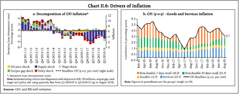 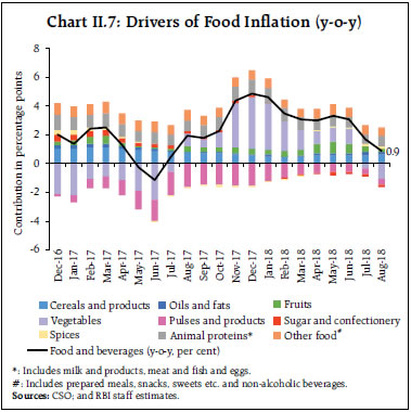 Vegetables account for 6 per cent of the CPI and 13.2 per cent of the food and beverages group. A delayed winter easing of price pressures in vegetables commenced from December 2017 and extended well up to April 2018, as mandi arrivals, specifically of onions and tomatoes, surged muting the usual summer upturn (Chart II.9a). Onion inflation declined from a high of 159 per cent in December 2017 to 23 per cent in May 2018, pulled down by bumper mandi arrivals, imports, and implementation of a minimum export price (MEP) that deterred exports, together creating persistent surplus supply conditions. Onion prices, however, picked up in July with the country-wide transporters’ strike, which affected the supplies of essential food items. After remaining low during April-May, prices of tomatoes recorded an upsurge during June-July due to widespread farmers’ agitations. By contrast, price pressures have been more pronounced in respect of potatoes since March 2018 due to lower availability of stocks from cold storages, transport disruptions and protests organised by potato farmers against not receiving remunerative prices for their crops. Prices of vegetables, however, witnessed some easing in August 2018 led by a contraction in prices of tomatoes and moderation in onion price pressures as arrivals surged, which played a key role in moderating food inflation during the month. 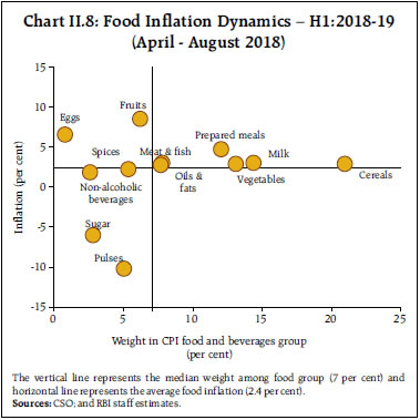 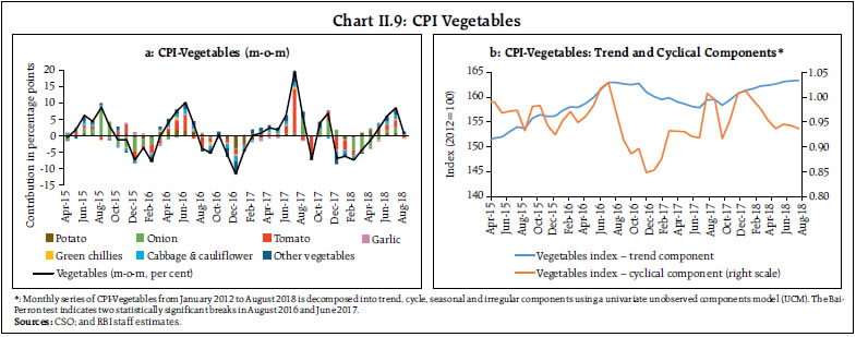 An analysis of prices of vegetables based on sectoral CPI indices suggests that there is no statistically significant difference in month-on-month changes in prices of vegetables between rural and urban areas.5 A decomposition of the CPI-vegetables into its trend and cyclical components reveals a rising trend since H1:2017-18, indicating that the recent softening in vegetable prices may not be structural in nature (Chart II.9b). Fruits prices also declined during June-August, contrary to the usual seasonal pattern. Fruits have a weight of 2.9 per cent in the CPI and 6.3 per cent within the food and beverages sub-component. Healthy domestic production of major fruits like mangoes and bananas, together with imports of some fruits (particularly apples and citrus fruits) pulled down fruits prices in contrast to the usual pattern in June and July every year when they rise (Chart II.10). 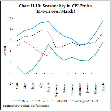 Deflation in the prices of pulses persisted on the back of over-supply, though the pace of deflation moderated during H1. Pulses account for 2.4 per cent of the CPI and 5.2 per cent of the food and beverages sub-component. Mandi level prices of some pulses such as arhar and urad remained below their minimum support prices (MSPs) in major producing states such as Maharashtra, Madhya Pradesh, Uttar Pradesh and Karnataka. In response, several measures that had been undertaken by the government in the previous year were extended into 2018-19 such as (i) removal of the export ban on all pulses; and (ii) imposition of import duty of 60 per cent on gram and 30 per cent on masoor to provide some relief to farmers. Nonetheless, pulses prices continued to rule well below their historical trend during H1:2018-19 (Chart II.11). Prices of sugar and confectionery also remained in deflation zone from February 2018 on account of surplus production during the sugarcane season of 2017-18 (Charts II.7 and II.8). Domestic sugar prices have closely tracked global price movements which have also been in deflation due to excess global supply. In view of the sharp decline in sugar prices, the government raised the import duty on sugar to 100 per cent, besides re-imposing stockholding limits on sugar sales and fixing the ex-mill sugar prices to ₹29 per kg in June 2018. Moreover, the customs duty on export of sugar was withdrawn to encourage the sugar industry. These measures, along with supply disruptions in July following the transporters’ strike, drove up sugar prices during June-August, though y-o-y inflation continued to be in the negative zone. 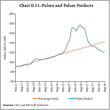 In the case of protein-rich items such as eggs, price pressures were visible during June-July 2018, reflecting the combined impact of the usual lower egg production during summer months and higher consumption during early monsoon months in several parts of the country. Furthermore, the country-wide truckers’ strike in July also affected the supply of eggs in several states, adding to upside pressures on prices. However, prices of eggs softened in August. Among other protein-rich items, meat and fish prices experienced the usual upside pressures during May-June, followed by easing during July-August. In the case of milk and products, price pressures were subdued due to robust growth in milk production. Among other food components, edible oil inflation recorded a pick-up in August 2018 after remaining in the range of one to three per cent since May 2017. After an increase in import duties on all major varieties of oils in November 2017, duties were hiked further during March and June 2018 in order to curb cheap imports. Inflation in spices started rising beginning April 2018 after remaining in deflation for 10 successive months since June 2017. While pressures on black pepper prices have remained muted so far, prices of other spices like dry chillies, turmeric, jeera, dhania and tamarind have firmed up, thereby driving up overall inflation in this group (Charts II.7 and II.8). On July 4, 2018 the central government announced minimum support prices (MSPs) for all kharif crops of a minimum of 150 per cent of the cost of production. Increases in MSPs generally get transmitted to headline inflation through direct and second round effects and, it is in the context of the upside risks to the near-term inflation outlook that the size and span of the impact of the MSP need to be carefully evaluated (Box II.1). CPI Fuel Group Fuel and light inflation increased sequentially every month from a trough of 5.2 per cent in April 2018 to 7.2 per cent by June 2018 and further to 8.5 per cent by August 2018 (Chart II.12a). Domestic prices of liquefied petroleum gas (LPG) tracked rising international product prices. Since the migration of subsidy payments on LPG to bank accounts under the direct benefit transfer scheme, LPG prices in CPI mirror open market prices. As such, they now reflect international prices closely (Chart II.12b). Inflation in respect of items of rural consumption such as firewood and chips continued to be sticky and elevated. Administered kerosene prices also registered sustained increases as oil marketing companies (OMCs) raised prices regularly in a calibrated manner. Box II.1: Assessing the Impact of MSPs on CPI Inflation Fulfilling the announcement made in the Union Budget 2018-19, MSPs for 14 crops for the 2018-19 kharif season were raised to at least 1.5 times of production (A2+FL) costs.6 This implies a nominal MSP increase in the range of 3.7 to 52.5 per cent for different crops over their levels a year ago, an area weighted increase of 17.3 per cent, a production weighted increase of 14.0 per cent, and a CPI weighted increase of 13.3 per cent (excluding cotton, as it does not appear directly in the CPI basket). In a historical perspective, the current increase in MSPs is significantly higher than the average of the last five years, but well below the upward revisions effected in 2008-09 and 2012-13 (Chart II.1.1). Empirically, it is observed that procurement is the channel through which higher MSPs pass through into inflation (RBI, 2018). For kharif crops, procurement has been the highest in respect of paddy at 32.4 per cent of production (average of last seven years), whereas it is negligible or absent in the case of other crops; an outlier was arhar for which procurement increased from insignificant levels to 23.7 per cent of production in 2016-17 as a part of the government’s food management strategy (Chart II.1.2). 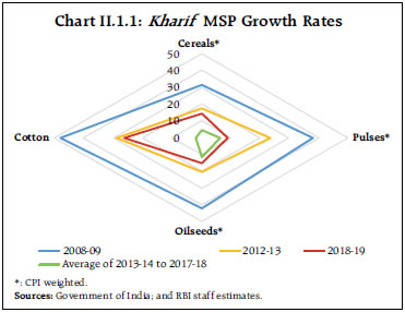 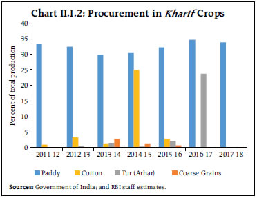 Estimates of the impact of the July 2018 MSP announcements on CPI inflation that are available in the public domain range from 20 bps to 110 bps. For operational purposes, however, precision in these estimates is the key since it conditions the monetary policy response to the likely deviations of inflation from its target. Illustratively, a straight-line approach of imputing the full increase in MSPs on to headline CPI inflation by using CPI weights for the crops in consideration, but without factoring in the scale of procurement operations, may overestimate the MSP impact. The total impact of MSPs on inflation comprises a first round (direct) effect and subsequent second (indirect) round effects. The first round effect – the quantum by which individual commodities respond to MSP shock – is estimated econometrically. The second-round effects are estimated using a two-stage process: (1) A static approach that mimics time-invariant economy-wide effects, is first employed to estimate the commodity level producer price effect through a series of iterations using input-output (IO) tables for 2012-13 and mapping those effects to the wholesale price index (WPI) using WPI weights; (2) The pass-through of the wholesale price increases to CPI food inflation components is then worked out by using elasticities derived from an Autoregressive Distributed Lag (ARDL) model. The second-round effects are also examined using RBI’s quarterly projection model, which is a new Keynesian open economy gap model. It attempts to capture several inter-twined effects dynamically. A hike in MSP could trigger relative price adjustments between MSP and non-MSP food items. Higher MSPs could also lead to a rise in rural incomes which would boost food demand. Furthermore, higher labour demand could lead to overall wage increases in the rural sector as labourers migrate from sowing/cropping of non-MSP to MSP crops. This increase in prices of food items, coupled with rising rural wages and incomes, could affect prices of non-food goods and services via second round effects (Ghate et al., 2018). The increase in the cotton MSP could directly affect inflation through retail clothing (Chart II.1.3). 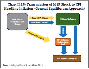 A first approximation of the inflationary impact of MSP increase from these methodologies yields 29-35 bps increase in headline CPI inflation. These estimates are highly tentative in the absence of robust information on the actual size and scale of procurement operations or more broadly on the combined effectiveness of procurement, price support/deficiency schemes and private sector participation as envisaged under the Pradhan Mantri Annadata Aay SanraksHan Abhiyan (PM AASHA) programme. Accordingly, these initial estimates need to be read with appropriate caveats and revisited once further details are released on actual MSP implementation. References: Benes, M. J., K. Clinton, A. T. George, P. Gupta, J. John, O. Kamenik, D. Laxton, P. Mitra, G. V. Nadhanael, R. Portillo, H. Wang and F. Zhang (2016). “Quarterly Projection Model for India: Key Elements and Properties”, RBI Working Paper, November. Ghate, C., S. Gupta, and D Mallick (2018). “Terms of Trade Shocks and Monetary Policy in India”, Computational Economics , Volume 51, Issue 1, pp 75–121, January. Reserve Bank of India (2018). “MSPs - Do They Influence Inflation Trajectory?”, Box II.2.2, RBI Annual Report 2017-18. |
 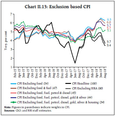 CPI Excluding Food and Fuel A sustained rise in CPI inflation excluding food and fuel started in H2:2017-18 and continued into H1:2018-19 – it rose from 5.1 per cent in February to 6.4 per cent in June, before moderating to 6.2 per cent in July and further to 6.0 per cent in August (Chart II.13). Adjusted for the estimated HRA impact, CPI inflation excluding food and fuel was 5.5 per cent in H1:2018-19 (up to August) – 70 bps lower than the actual outcome. Housing inflation contributed close to 30 per cent of the increase in CPI inflation excluding food and fuel in H1:2018-19 (up to August), largely reflecting the HRA increases of central government employees (Chart II.14). Adjusted for HRA, the housing group still contributed a fifth of overall increase in CPI inflation excluding food and fuel. The second largest contributor in this category was the transport and communication sub-group, largely reflecting increases in petrol and diesel pump prices and second-round effects on transport fares. Petrol (and diesel) pump prices during H1:2018-19 increased sharply by about ₹10 per litre, as international prices surged (Chart II.15). As a result, the contribution of petrol and diesel (with a weight of 2.3 per cent) to CPI excluding food and fuel inflation rose from 1.7 per cent in March 2018 to 8.6 per cent in August. Accentuating the impact of petrol and diesel on inflation in the recent period has been the asymmetric pass-through of international crude oil prices to domestic prices since 2014 (Chart II.15). 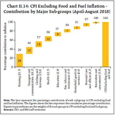 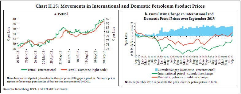 Excluding food, fuel, petrol and diesel, CPI inflation increased from 5.2 per cent in February to peak at 6.2 per cent in June, before moderating to 5.8 per cent in July and to 5.7 per cent in August. Excluding the four volatile items – petrol, diesel, gold and silver – as well as housing, CPI inflation increased by 120 bps from February to 5.5 per cent in June, before moderating to 5.0–5.1 per cent in July–August (Chart II.13). The edging down of inflation in July and August was due to lower inflation prints in pan, tobacco and intoxicants, clothing and footwear, and miscellaneous groups. Inflation in respect of both goods and services in the CPI excluding food, fuel, petrol and diesel edged up during Q1:2018-19 (Chart II.16). For goods, inflation picked up across commodity groups, particularly medicines, clothing and footwear, bedding, utensils and washing powder. However, during July-August 2018, goods inflation moderated sharply by 80 bps, driven primarily by a fall in inflation in pan, tobacco and intoxicants group and personal care and effects sub-group (Chart II.16a). Services inflation rose in H1:2018-19 to reach a peak of 6.9 per cent in June, driven up largely by the HRA increases and an increase in tuition fees and prices of transportation services, as alluded to earlier. As the HRA effects started to wane, services inflation moderated to 6.5 per cent in August (Chart II.16b). Excluding the HRA impact, services inflation rose from 5.0 per cent in March and remained steady at 5.5 per cent during June-August. Communication services inflation, however, remained muted due to subdued prices in respect of cellular services. 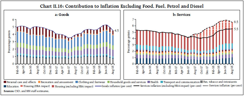 Other Measures of Inflation Measures of inflation other than the CPI have shown mixed movements since the April MPR. After the HRA-linked spike in January 2018, inflation in terms of CPI for industrial workers (CPI-IW) declined in line with inflation in CPI for agricultural labourers (AL) and rural labourers (RL), reflecting inter alia soft food inflation readings. CPI-IW reflects changes in its housing index once in six months – in January and July every year. The revision in CPI-IW housing index – from 3.0 per cent in December 2017 to 10.2 per cent in January 2018 and further to 26.1 per cent in July – created sizeable upside impulses pushing CPI-IW inflation significantly above headline CPI inflation in July.7 Accordingly, as the impact of the HRA increase intensified, CPI-IW inflation shot up to 5.6 per cent in August from 3.9 per cent in June. In contrast, wholesale price index (WPI) inflation firmed up significantly in Q1, driven up by international prices of crude petroleum and high speed diesel. Inflation in respect of electricity, naphtha, furnace oil, manufacture of plastic products, manufactured vegetable and animal oils and fats also fuelled WPI inflation. GDP and GVA deflators also ticked up in Q1 in line with WPI inflation (Chart II.17a) which moderated somewhat in July and August with the collapse in food inflation. Volatile prices of items such as transport fuel, vegetables, pulses and precious metals impart high dispersion, asymmetry and non-normality to the distribution of inflation. High positive as well as negative skew and chronic fat tails in the inflation distribution could be removed by trimming the outliers. Trimmed means of CPI, including its weighted median, rose sharply in Q1:2018-19 before softening in July and August (Chart II.17b). II.3 Costs Measures of inflation have largely tracked underlying cost conditions. In the case of industrial and farm costs in the WPI and remained elevated in Q2 so far (Chart II.18). The rise in global crude oil prices impacted domestic prices of inputs such as high speed diesel, aviation turbine fuel, naptha, bitumen, furnace oil and petroleum coke, pushing up domestic farm and nonfarm costs. Input cost pressures weakened slightly in July 2018, reflecting soft metal prices and transient easing of global crude oil prices. 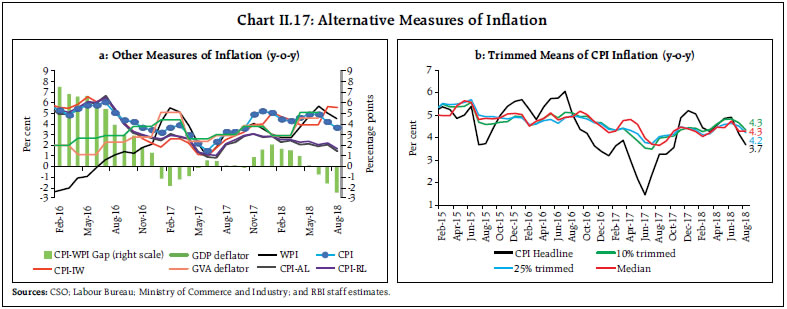 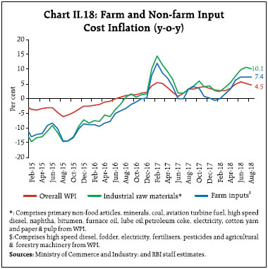 Among other industrial raw materials, domestic coal inflation slowed down significantly as compared with the previous year’s level. Inflation in respect of paper and paper products has also remained moderate so far, reflecting inter alia cheap imports of paper under free trade agreements with the Association of Southeast Asian Nations (ASEAN) and South Korea. Inflation in prices of fibres (specifically cotton, jute and mesta) after remaining in negative territory during February to May 2018, picked up subsequently due to elevated international prices and lower production estimates for 2018-19 season. Among farm sector inputs, inflation in respect of agricultural input prices such as fertilisers increased gradually in line with international prices. Despite rising demand, prices of tractors remained stable on the back of increased competition as tractor firms aspired to expand their market shares. Inflation in respect of pesticides and other agrochemical products was driven by uptick in inflation in insecticide and pesticide even as deflation in fungicide prices continued. Prices of fodder remained in deflation due to increased production on the back of good monsoons during the last two years. Inflation in respect of electricity, which has a high weight in both industrial and farm inputs, rose significantly during May-August, reflecting mainly the price surge on account of supply disruptions in the summer following severe dust storms in northern India and adverse base effect in August. Additionally, the distribution companies (DISCOMS) raised their tariffs, following the diversion of coal supplies by the government away from captive power producers to thermal power plants with low stocks. Growth in rural wages, both for agricultural and non-agricultural labourers, has remained subdued since August 2017, reflecting the lagged impact of low inflation in the previous few months (Chart II.19). Pressure from staff costs in the organised sector has broadly been contained. The uptick in staff costs growth in the manufacturing sector in Q4 was short-lived and it slid back in Q1:2018-19. The annual growth in per employee cost for the manufacturing sector stood at 11.4 per cent in Q1:2018-19. For the services sector, the sequential deceleration since Q4:2015-16 in staff cost growth was interrupted by an uptick in Q1:2018-19 when it rose by 9.8 per cent (Chart II.20a). Unit labour costs for companies in the manufacturing sector have been volatile and remained muted in Q1:2018-19.8 Unit labour costs in the services sector edged down in Q1, with the growth in value of production outpacing the growth of staff cost (Chart II.20b). Pressure from rising commodity prices was also reflected in an increase in input costs of manufacturing firms covered in the Reserve Bank’s industrial outlook survey. These firms reported a rise in the cost of raw materials in Q2:2018-19 and expected it to increase further in Q3. However, they are not expecting to pass the entire cost burden to selling prices, reflecting still subdued pricing power. The manufacturing purchasing managers’ index (PMI) as well as the services PMI point to an increase in the cost of raw materials in Q1 and Q2 so far. Firms covered in these indices also reported an increase in their selling prices, indicating that some pass-through of higher costs to clients may already be occurring. II.4 Conclusion Going forward, inflation outcomes will be influenced by several factors. The government has announced measures aimed at ensuring remunerative prices to the farmers for their produce. The magnitude of the impact of these measures on CPI inflation will be contingent upon the manner and effectiveness with which these measures are implemented. Risks to inflation could emanate from rising geopolitical and trade tensions, with attendant implications for global commodity prices and financial markets. The impact of the 7th CPC HRA award on headline inflation has started waning and the effect of increases in HRA by states is not yet visible. As and when HRA awards by states start showing up in the CPI, it will impact headline inflation. As in the case of the centre’s HRA, second round effects will warrant vigilance. The near-term inflation expectations of households and those of businesses polled in the forward-looking surveys of the Reserve Bank of India have firmed up over successive rounds, with the potential to feed into wages and input costs. While low food inflation prints and the positive outlook on food – on account of supply management measures by government and a normal monsoon – provide comfort, it is necessary to be watchful as several upside risks to inflation persist, notably from surging oil prices and volatile financial markets.
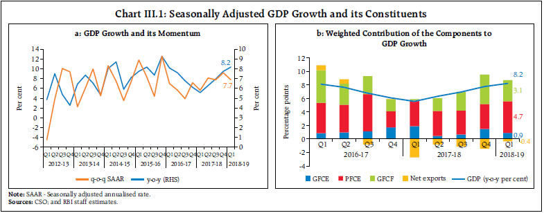
III. Demand and Output Aggregate demand has been underpinned by the strengthening of private consumption and investment demand. The drag from external demand has reduced with a robust pick-up in non-oil merchandise exports. Aggregate supply conditions improved with a sharp acceleration in manufacturing and the resilience in agriculture and allied activities. Raising real investment activity on a durable basis holds the key to sustaining the growth momentum, going forward. Since the start of 2018, i.e., from the January-March 2018 quarter, economic activity in India appears to be charting a step-up in its trajectory. Quarterly estimates of the Central Statistics Office (CSO) for Q1:2018- 19 (April-June) confirm that gross domestic product (GDP) growth averaged 8 per cent in the January-June 2018 period, up from 6.6 per cent in the period July- December 2017. High frequency and survey-based indicators suggest that aggregate demand is fast catching up with aggregate supply. Sales growth, pick-up in capacity utilisation and the acceleration in the fast-moving consumer goods (FMCGs) space attest that the output gap has virtually closed. Meanwhile, another engine of aggregate demand has started to pick-up with the bounce-back in merchandise exports. On the supply side, the rapid catch-up in sowing activity, backed by ample reservoir storage, brightens the outlook for agriculture and allied activities on top of the record production in 2017-18. Industrial activity has strengthened and become more broad-based, buoyed by manufacturing. The services sector remains resilient, supported by strong growth in construction activity as well as public administration, defence and other services (PADO). III.1 Aggregate Demand Measured by year-on-year (y-o-y) changes in real GDP at market prices, aggregate demand strengthened to 7.7 per cent in Q4:2017-18 and surged to a nine-quarter high of 8.2 per cent in Q1:2018-19 (Table III.1). This extended its sequential acceleration to four successive quarters, beginning in Q2:2017-18. Momentum, measured by q-o-q seasonally adjusted annualised rate (SAAR), however, moderated in Q1:2018-19 (Chart III.1a). Among its components, consumption expanded on the back of growth in private final consumption expenditure (PFCE), which reached a six-quarter high of 8.6 per cent in Q1:2018-19. Government final consumption expenditure (GFCE) decelerated to 7.6 per cent, albeit from a high of 16.9 per cent in Q4:2017-18. Investment demand embodied in the growth of gross fixed capital formation (GFCF) decelerated sequentially in Q1:2018-19; however, it remained reasonably strong at 10 per cent, given the government’s thrust on national highways and low-cost housing. Despite a hostile and unpredictable international trading environment, growth of exports of goods and services jumped to a 16-quarter high of 12.7 per cent in Q1:2018-19, mitigating the negative contribution of net exports to aggregate demand caused by the unrelenting surge in imports (Chart III.1b). | Table III.1: Real GDP Growth | | (Per cent) | | Item | 2016-17 | 2017-18 (PE) | Weighted Contribution* | 2016-17 | 2017-18 (PE) | 2018-19 | | 2016-17 | 2017-18 | Q1 | Q2 | Q3 | Q4 | Q1 | Q2 | Q3 | Q4 | Q1 | | Private final consumption expenditure | 7.3 | 6.6 | 4.1 | 3.7 | 8.3 | 7.5 | 9.3 | 4.2 | 6.9 | 6.8 | 5.9 | 6.7 | 8.6 | | Government final consumption expenditure | 12.2 | 10.9 | 1.2 | 1.1 | 8.3 | 8.2 | 12.3 | 22.5 | 17.6 | 3.8 | 6.8 | 16.9 | 7.6 | | Gross fixed capital formation | 10.1 | 7.6 | 3.1 | 2.4 | 15.9 | 10.5 | 8.7 | 6.0 | 0.8 | 6.1 | 9.1 | 14.4 | 10.0 | | Exports | 5.0 | 5.6 | 1.0 | 1.1 | 3.6 | 2.4 | 6.7 | 7.0 | 5.9 | 6.8 | 6.2 | 3.6 | 12.7 | | Imports | 4.0 | 12.4 | 0.9 | 2.7 | 0.1 | -0.4 | 10.1 | 6.6 | 18.5 | 10.0 | 10.5 | 10.9 | 12.5 | | GDP at market prices | 7.1 | 6.7 | 7.1 | 6.7 | 8.1 | 7.6 | 6.8 | 6.1 | 5.6 | 6.3 | 7.0 | 7.7 | 8.2 | PE: Provisional Estimates.
*: Component-wise contributions do not add up to GDP growth in the table because changes in stocks, valuables and discrepancies are not included.
Source: Central Statistics Office (CSO), Government of India. |
 The April 2018 MPR had projected real GDP growth of 7.3 per cent for Q1:2018-19, with risks evenly balanced around the baseline path (Chart III.2). 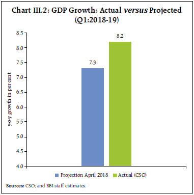 The actual outcome for the quarter overshot the projection by 90 basis points, reflecting larger than expected gains in most of the constituents of aggregate demand. First, private consumption demand surprised on the upside in Q1:2018-19 and touched a six-quarter peak. The April 2018 projection had assumed that lingering effects of the goods and services tax (GST) implementation would have an adverse impact on consumption demand – especially in urban areas – through loss of output and employment in unorganised activities. Furthermore, a sharp acceleration in allied activities in the agricultural sector posted a growth of 8.1 per cent in Q1:2018-19, which was significantly above trend. This is likely to have boosted rural consumption. Second, GFCF growth overshot the projection on account of stronger than expected capital goods production and the robust recovery in the construction sector. III.1.1 Private Final Consumption Expenditure PFCE remained the mainstay of aggregate demand running ahead in Q1:2018-19 on the strength of rising rural and urban demand and undeterred by the surge in domestic prices of petroleum products. After rising since the beginning of 2017-18, wage (staff cost per employee) growth in the organised manufacturing and services sectors has remained range bound (see Chart II.20, Chapter II). However, in the information technology (IT) sector, growth in staff cost was robust in Q1:2018-19, which could have added to the purchasing power. In contrast, anecdotal evidence suggests that following a decline in exports and moderation in domestic production, growth in wage incomes could have moderated in some of the labour-intensive segments such as readymade garments, and jute manufactures, which, in turn, might have impacted consumption demand (Chart III.3).  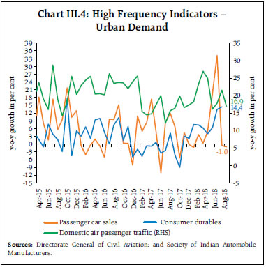 High frequency indicators of urban consumption present a mixed picture. While domestic air passenger traffic and production of consumer durables expanded during Q1 and Q2:2018-19 so far, sales of passenger cars contracted during July-August, after peaking in June, possibly as a response to the sharp rise in fuel prices (Chart III.4). Household credit demand in the form of personal loans and leasing of vehicles by commercial banks maintained a robust tempo (Chart III.5). Going forward, urban consumption is expected to strengthen further on the implementation of the 7th Central Pay Commission (CPC) awards by states and the recent reduction in GST rates. High frequency indicators of rural demand seem to be indicating a slight loss of momentum in Q2:2018- 19 (Chart III.6). Sales of motorcycles and tractors, which grew robustly during Q1:2018-19, decelerated in Q2 (July-August). Nevertheless, construction activity in rural areas has been buoyant since Q2:2017-18, supported by the government’s thrust on rural housing and roads. Strong topline growth of FMCG companies, a sizeable part of which emanates from rural areas, also corroborates the improving dynamics of rural consumption. The latter should also benefit from the tailwinds of normal rains in large parts of the country, given the empirical evidence of a positive association of normal monsoon with growth in private consumption (Chart III.7).1 The sizeable increase in MSP of kharif crops announced in July 2018 is expected to augment incomes of rural households if it is implemented effectively. III.1.2 Gross Fixed Capital Formation Growth in gross fixed capital formation (GFCF), which had accelerated to a seven-quarter high of 14.4 per cent in Q4:2017-18, retained double-digit growth in Q1:2018-19 with some moderation in pace relative to the previous quarter. The share of GFCF in aggregate demand in Q1:2018-19 at 31.6 per cent was higher than 31.0 per cent a year ago, indicating improving investment demand. Robust investment activity was also reflected in several high frequency indicators such as steel consumption, cement production, and import of capital goods (Chart III.8). Strong growth in housing loans disbursed by scheduled commercial banks (SCBs) and especially housing finance companies also suggests rising investment in the construction sector. 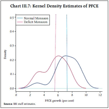 Capacity utilisation (seasonally adjusted) gained momentum and improved to 74.9 per cent in Q1:2018- 19, higher than the level recorded in the first quarter of the past year (Chart III.9). The number of stalled projects, though reported some improvement in both the private and government sectors in Q4:2017-18 and Q1:2018-19, there was a slight deterioration in government sector in Q2:2018-19 (Chart III.10). Since 2011-12, capital formation has decelerated due to the slowdown in investment in the private sector, weighed down, inter alia, by overhang of corporate debt (Chart III.11). Empirical analysis suggests that higher leverage constrains firms’ ability to invest, resulting in slowdown in fresh investment (Box III.1). Since H2:2017-18, however, the corporate sector has been deleveraging, especially in the manufacturing sector, which is reflected in an improvement in their interest coverage ratios (ICRs) (Chart III.12). Recent data on investment activity and several lead/coincident indicators of investment, viz., sales growth, capacity utilisation, inventory drawdown, and gradually returning pricing power suggest that the investment cycle has turned.2 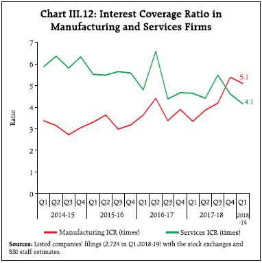
Box III.1: Leverage and Investment Empirical evidence on firm-level capital investment points to sales growth, leverage, growth of debt and repaying capacity of firms being its key determinants (Krznar and Matheson, 2018; Li, Magud and Valencia, 2015; Magud and Sosa, 2015). Leverage, which affects investment behaviour in multiple ways, constrains a firm’s capacity to mobilise external resources for financing new and risky projects. In a scenario of high leverage, major gains from investment accrue to debt-holders, thereby discouraging promoters from undertaking further investment. In the aftermath of the global financial crisis, leverage of Indian non-financial firms, measured as the ratio of debt to equity, rose across sectors, eroding debt servicing capacity and undermining investment decisions. In order to formally examine the impact of leverage on investment activity, firm-level data of both listed and non-listed non-financial companies for the period of 2004 to 2017 drawn from the CMIE’s Prowess database were modelled in a dynamic Arellano-Bond panel regression framework that addresses the problem of potential endogeneity of regressors: The results confirm the dominant negative influence of leverage in determining fixed investment while sales growth, operating profit and market price to book value positively affect investment (Table III.1.1). One percentage point increase in leverage was found to reduce fixed investment by 40 basis points. The specification was also tested at sectoral level, viz., manufacturing, construction and metals. The sectoral results also corroborate the aggregate findings. The growth of outstanding debt is found to have a positive impact on capital expenditure as firms finance long-term investment by incurring new debt. Sales growth, an indicator of current and future demand, also leads to further investment, supporting that the investment accelerator is at work. | Table III.1.1: Regression Results – Impact of Leverage over Firms’ Capital Expenditure (2004-2017) Dependent Variable: Investment-Fixed Asset Ratio | | | Overall | Manufacturing Firms | Construction Sector Firms | Metal Sector Firms | | | (1) | (2) | (3) | (4) | | Investment ratio (lag) | 0.133*** | 0.138*** | 0.043 | 0.112*** | | | (0.010) | (0.015) | (0.038) | (0.020) | | Debt to equity ratio | -0.399*** | -0.197** | -1.924*** | -0.241 | | | (0.093) | (0.095) | (0.581) | (0.198) | | Interest coverage ratio | 0.005 | -0.005 | 0.027* | 0.001 | | | (0.003) | (0.004) | (0.015) | (0.008) | | Sales growth rate (y-o-y) | 0.020*** | 0.020* | 0.016*** | 0.032*** | | | (0.002) | (0.010) | (0.005) | (0.012) | | Growth of operating profit (y-o-y) | -0.000 | -0.002 | 0.004 | -0.001 | | | (0.001) | (0.001) | (0.006) | (0.002) | | Growth of outstanding debt (y-o-y) | 0.011*** | 0.012*** | 0.005 | 0.015*** | | | (0.001) | (0.002) | (0.005) | (0.004) | | Market price to book value ratio (annual average) | 0.249** | -0.015 | 1.182*** | -0.189 | | | (0.103) | (0.114) | (0.391) | (0.252) | | Constant | 5.553*** | 7.077*** | 3.392*** | 8.453*** | | | (0.299) | (0.310) | (0.992) | (0.561) | | Observations | 20,726 | 13,885 | 1,421 | 4,673 | | Number of firms | 2,693 | 1,669 | 191 | 558 | Note: *** p<0.01, ** p<0.05, * p<0.1.
Source: RBI staff estimates. | To conclude, high leverage among non-financial firms leads to a slowdown of investment in the economy. Recent concerted efforts to strengthen balance sheets of both firms and banks are expected to lead to pick-up in capital formation in the medium to long term. References: Krznar, I., and T. Matheson (2018), Investment in Brazil: From Crisis to Recovery, IMF Working Paper, WP/18/6. Li, D., N. Magud and F. Valencia (2015), Corporate Investment in Emerging Markets: Financing vs. Real Options Channel, IMF Working Paper, WPIEA2015285. N. Magud and S. Sosa (2015), Investment in Emerging Markets: We Are Not in Kansas Anymore…Or Are We?, IMF Working Paper, WP/15/77. | III.1.3 Government Expenditure GFCE continued to support aggregate demand in Q1. The fiscal position of the central government showed an improvement in terms of key deficit indicators, as per cent of budget estimates (BE), during April-August 2018-19 as growth in revenue receipts exceeded that of expenditure (Table III.2). Tax revenues grew by 7.5 per cent, supported by higher income tax collections (Charts III.13a and b). Notwithstanding month-over-month fluctuations, the overall indirect tax base has expanded. Ongoing simplification of procedures and rationalisation of GST rates have encouraged voluntary compliance, especially in the business-to-business segment and small enterprises. Many registrants under the GST network (GSTN) were those who fell below the GST threshold but nevertheless chose to be a part of the GST. Similarly, more than 50 percent of those who could have chosen to opt for the simpler composition scheme chose to register under the regular GST scheme.3 States’ own tax revenues, comprising mainly their collection under the state goods and services tax (SGST), have stabilised in recent months, though there is some uncertainty relating to the sharing of revenues from the integrated goods and services tax (IGST) between the centre and states and the transfer under GST compensation cess.4 Furthermore, non-tax revenues have shown a marked improvement for centre. | Table III.2: Key Fiscal Indicators – Central Government Finances (April-August) | | (Per cent) | | Indicator | As a per cent of BE | y-o-y Growth | | 2017-18 | 2018-19 | 2018-19 | | 1. Revenue receipts | 27.0 | 26.9 | 13.3 | | a. Tax revenue (Net) | 27.8 | 24.7 | 7.5 | | b. Non-tax revenue | 24.0 | 40.1 | 42.0 | | 2. Total non-debt receipts | 26.6 | 26.4 | 12.7 | | 3. Revenue expenditure | 45.8 | 43.8 | 11.6 | | 4. Capital expenditure | 35.4 | 44.0 | 20.6 | | 5. Total expenditure | 44.3 | 43.8 | 12.7 | | 6. Gross fiscal deficit | 96.1 | 94.7 | 12.6 | | 7. Revenue deficit | 134.2 | 114.0 | 10.0 | | 8. Primary deficit | 1401.3 | 767.7 | 13.2 | BE: Budget Estimates.
Source: Controller General of Accounts, Ministry of Finance, Government of India and Union Budget Document, 2018-19. | On the expenditure front, accounts for April-August 2018-19 reveal a marked moderation in revenue expenditure mainly due to lower subsidy outgo. The quality of expenditure improved, with growth in capital expenditure – at 20.6 per cent – outpacing revenue expenditure. As regards states, the share of revenue expenditure in their total expenditure was estimated slightly lower at 83 per cent in their BE for 2018-19, though still higher than in 2015-16 and 2016-17 (Table III.3).
| Table III.3: Revenue Expenditure, Interest Payments and Indebtedness of All States | | (Per cent) | | Year | Revenue Expenditure / Total Expenditure | Interest Payment / Revenue Expenditure | Debt / GSDP | | 2015-16 | 81.3 | 11.7 | 23.4 | | 2016-17 | 80.4 | 12.0 | 23.8 | | 2017-18 (RE) | 83.2 | 11.6 | 24.0 | | 2018-19 (BE) | 82.9 | 11.3 | 24.3 | | Source: RBI staff estimates. | There is a positive relationship between indebtedness of states (debt/GSDP) and their respective shares of revenue expenditure in total expenditure. This relationship is stronger in the case of non-special category states than in special category states5 (Chart III.14). States with high interest burden (higher interest payment as per cent of revenue expenditure) find it more difficult to control their revenue expenditure, thereby putting a strain on the quality of expenditure. During 2017-18, the combined fiscal position of the centre and states deteriorated vis-à-vis BE due to elevated revenue expenditure and subdued growth in revenue collection resulting from the teething problems with the GST implementation. Consequently, the fiscal deficit of centre and states deviated significantly from BE. The combined gross fiscal deficit (GFD) is budgeted to decline to 5.9 per cent of GDP in 2018-19 from 6.6 per cent in the revised estimates (RE) for 2017-18. Outstanding liabilities of the general government (centre and states) are budgeted to decline to 68.3 per cent of GDP by end-March 2019 from 68.9 per cent a year ago (RE).6 Concerted efforts towards consolidation will, however, be needed for achieving the revised Fiscal Responsibility and Budget Management (FRBM) targets, i.e., the central government debt to GDP ratio of 40 per cent and the general government debt to GDP ratio of 60 per cent by 2024-25. 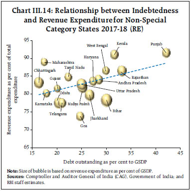 The Reserve Bank managed the centre’s market borrowing programme during 2018-19 so far as per the planned issuance schedule, despite reduced demand for government securities from foreign portfolio investors (FPIs). Against the budgeted market borrowing for 2018-19 at ₹6,055 billion (about 3 per cent higher than last year), the central government completed 47.6 per cent of its budgeted gross borrowings by end-September 2018 (64.1 per cent in the corresponding period of 2017-18). It decided not to front-load market borrowings in the first half of the year in a departure from the typical pattern of market borrowings (Table III.4). It has decided to reduce its budgeted market borrowings in the second half of the year by ₹705 billion, which will take the market borrowings for the full year to ₹5,350 billion against the budgeted ₹6,055 billion. The government expects that higher inflows in the National Small Savings Fund (NSSF) scheme and adjustments in buyback programme would enable it to meet the budgeted fiscal deficit target even with lower market borrowings. The states completed 27.6 per cent of their budgeted gross borrowings by end-September 2018 as against 36.7 per cent in the corresponding period of 2017-18. The bulk of market borrowings by the states would be in the second half of 2018-19. | Table III.4: Government Market Borrowings | | (₹ billion) | | | 2016-17 | 2017-18 | 2018-19 (end-September 2018) | | Centre | States | Total | Centre | States | Total | Centre | States | Total | | Net borrowings | 4,082 | 3,427 | 7,509 | 4,484 | 3,403 | 7,887 | 2,004 | 1,376 | 3,380 | | Gross borrowings | 5,820 | 3,820 | 9,640 | 5,880 | 4,191 | 10,071 | 2,880 | 1,575 | 4,455 | | Source: Government of India and RBI staff estimates. | A major challenge for government finances is adherence to the budgeted revenue expenditure, given impending elections in several states as well as for the centre. An analysis of GFCE growth for the period 1991-92 to 2017-18 suggests that it generally picks up in election years (Chart III.15). This highlights the risks of curtailment of capital expenditure and/ or deviation from the GFD targets. There are also risks of overshooting of revenue expenditure in the current year due to potential outlays associated with food and fuel subsidies for the centre, debt waivers for states, and the announced increase in minimum support price (MSP) for kharif crops. However, the government has indicated that it does not anticipate any slippage in the fiscal deficit target and expects the revenue collection to be in line with the budget estimates. 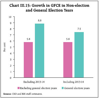 Revenue mobilisation through better tax compliance, non-tax revenues and disinvestment holds the key to sustaining fiscal consolidation by the centre. State finances are likely to be under pressure during the current fiscal year due to rollout of farm loan waivers and implementation of impending pay commission awards and arrears. III.1.4 External Demand Net exports continued to drag down aggregate demand in Q1:2018-19, though on a smaller scale than in the previous four quarters. India’s merchandise exports recovered smartly from the implementation effects of the GST and rode on improving global demand to expand at 14.6 per cent in US dollar terms in Q1:2018-19, a step-up from the average of 10.1 per cent in the previous four quarters (Chart III.16a). The recovery in export growth was strongly supported by non-oil exports such as engineering goods, chemicals and drugs and pharmaceuticals (Chart III.17a). Oil exports too expanded, but mainly on the back of a surge in international crude oil prices. Merchandise import growth during Q1:2018-19 was the slowest in four quarters on account of an unfavourable base effect and a decline in gold imports. There was also some moderation in non-oil non-gold imports with the decline in imports of pearls and precious stones, pulses and vegetable oil (Chart III.17b). The combined impact of the escalation in international crude oil prices and a pick-up in import volumes pushed up the oil import bill to a 15-quarter high. Notwithstanding the improved export performance, India’s merchandise trade deficit during Q1:2018-19 was the highest in last 20 quarters. During July-August 2018-19, both export and import growth improved. Exports benefitted from increased shipments of petroleum products, engineering goods and gems and jewellery. Petroleum, gold, coal and electronic goods supported import growth. 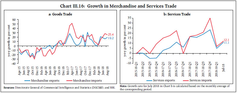 In Q1:2018-19, 65 per cent of India’s merchandise trade deficit was financed through invisibles, i.e., net export of services, income and remittances. Net services exports grew by 2.1 per cent on a y-o-y basis, primarily driven by exports of software and financial services. In gross terms, India’s services export recorded a growth of 4.9 per cent in Q1:2018-19 (Chart III.16b). India accounts for a large share (13.1 per cent share in total exports of the top 10 exporting economies)7 of global exports of telecommunications, computer and information services. Major IT companies reported significant improvement in their export revenues in Q1:2018-19, which might also have extended into Q2:2018-19 in view of the weakness of the rupee. Optimistic forecasts of global IT spending in 2018 also bode well for the outlook for software exports. Net remittances – mainly private transfers, which supplement gross domestic disposable income – rose by 17.5 per cent in Q1:2018-19, reflecting firmer demand conditions in source countries as also rising international crude oil prices, both of which imply a favourable outlook for these flows. Despite increase in net receipts of services exports and remittances in Q1:2018-19, trade deficit caused a slight widening of the current account deficit to US$ 15.8 billion (2.4 per cent of GDP) as compared with US$ 15.0 billion (2.5 per cent of GDP) in Q1:2017-18. 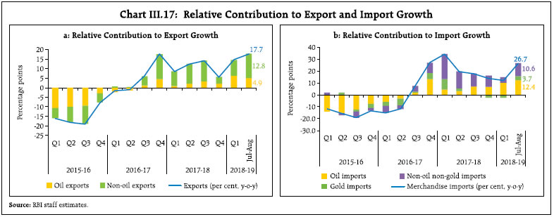 The global growth and trade outlook is clouded by rising protectionist tensions. The direct impact of the recently announced tariffs by the US on India’s exports is likely to be modest;8 however, the increase in US tariffs could lead to a supply glut in non-US markets and push prices down, resulting in lower export realisations for third party exporters like India. These risks appear to be materialising as the affected countries retaliate and protect domestic markets as already evident in tit-for-tat tariffs by the US and China. These developments could lead to a global trade slowdown with hysteresis, which, in turn, could diminish welfare, especially for countries looking to leverage on global trade to meet their growth aspirations. As regards financial flows in 2018-19 so far, net foreign direct investment (FDI) flows increased by 2.9 per cent in April-July 2018 over the corresponding period of the previous year. By contrast, FPI flows recorded net outflows of US$ 11.5 billion till September 28, 2018, reflecting mainly global portfolio rebalancing away from EMEs. While net receipts on account of non-resident deposits almost tripled in Q1:2018-19 from their level a year ago, both external commercial borrowings (ECBs) and short-term trade credit recorded outflows during the same period. Keeping in view the capital needs of the corporate sector, all-in-cost norms and end-use provisions were rationalised and the list of eligible borrowers was expanded for ECBs in April 2018. Despite the drawdown of reserves since April 2018, India’s forex reserves at US$ 400.5 billion as on September 28, 2018 were at a comfortable level – equivalent to 10 months of imports and 182 per cent of short-term external debt (by residual maturity). III.2 Aggregate Supply The growth of gross value added (GVA) at basic prices accelerated to an eight-quarter high of 8 per cent in Q1:2018-19 (Table III.5). However, GVA’s momentum, measured in terms of seasonally adjusted q-o-q annualised growth, somewhat weakened, suggesting that favourable base effects were primarily at work (Chart III.18). | Table III.5: Sector-wise Growth in GVA | | (Per cent) | | Sector | 2016-17 | 2017-18 (PE) | Weighted Contribution | 2016-17 | 2017-18 (PE) | 2018-19 | | 2016-17 | 2017-18 | Q1 | Q2 | Q3 | Q4 | Q1 | Q2 | Q3 | Q4 | Q1 | | Agriculture, forestry and fishing | 6.3 | 3.4 | 1.0 | 0.5 | 4.3 | 5.5 | 7.5 | 7.1 | 3.0 | 2.6 | 3.1 | 4.5 | 5.3 | | Industry | 8.7 | 5.5 | 2.0 | 1.3 | 10.2 | 7.8 | 8.8 | 8.1 | -0.4 | 7.1 | 7.3 | 8.0 | 10.8 | | Mining and quarrying | 13.0 | 2.9 | 0.4 | 0.1 | 10.5 | 9.1 | 12.1 | 18.8 | 1.7 | 6.9 | 1.4 | 2.7 | 0.1 | | Manufacturing | 7.9 | 5.7 | 1.4 | 1.0 | 9.9 | 7.7 | 8.1 | 6.1 | -1.8 | 7.1 | 8.5 | 9.1 | 13.5 | | Electricity, gas, water supply and other utilities | 9.2 | 7.2 | 0.2 | 0.2 | 12.4 | 7.1 | 9.5 | 8.1 | 7.1 | 7.7 | 6.1 | 7.7 | 7.3 | | Services | 6.7 | 7.6 | 4.1 | 4.7 | 8.5 | 7.4 | 6.0 | 4.9 | 8.5 | 6.4 | 7.5 | 8.2 | 7.5 | | Construction | 1.3 | 5.7 | 0.1 | 0.4 | 3.0 | 3.8 | 2.8 | -3.9 | 1.8 | 3.1 | 6.6 | 11.5 | 8.7 | | Trade, hotels, transport, communication | 7.2 | 8.0 | 1.4 | 1.5 | 8.9 | 7.2 | 7.5 | 5.5 | 8.4 | 8.5 | 8.5 | 6.8 | 6.7 | | Financial, real estate and professional services | 6.0 | 6.6 | 1.3 | 1.4 | 10.5 | 8.3 | 2.8 | 1.0 | 8.4 | 6.1 | 6.9 | 5.0 | 6.5 | | Public administration, defence and other services | 10.7 | 10.0 | 1.3 | 1.3 | 7.7 | 8.0 | 10.6 | 16.4 | 13.5 | 6.1 | 7.7 | 13.3 | 9.9 | | GVA at Basic Prices | 7.1 | 6.5 | 7.1 | 6.5 | 8.3 | 7.2 | 6.9 | 6.0 | 5.6 | 6.1 | 6.6 | 7.6 | 8.0 | PE: Provisional Estimates.
Source: CSO. |
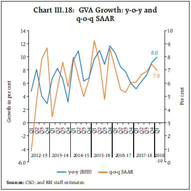 The acceleration of GVA growth was underpinned by manufacturing activity registering double-digit growth after eight quarters. Agricultural growth also accelerated on the back of double-digit growth in production of key crops during the rabi season, and sustained expansion in livestock products, forestry and fisheries during the quarter. There was some moderation in growth of services sector activity, essentially due to a high base. Construction activity maintained strong pace for the second consecutive quarter. Continued expansion in PADO was fuelled by an increase in government expenditure in Q1:2018- 19 (Chart III.19). III.2.1 Agriculture Agriculture and allied activities accelerated for the third consecutive quarter in Q1:2018-19, supported by higher production of rice, wheat, coarse cereals, pulses and oilseeds during the rabi season. As per the third advance estimates for 2017-18, horticulture production increased by 2.1 per cent, reaching a record of 306.8 million tonnes. The livestock products, forestry and fisheries sub-sector, which constituted around 45 per cent of GVA of agriculture and allied activities, grew at a robust rate of 8.1 per cent in Q1:2018-19. 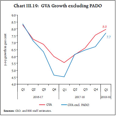 The fourth advance estimates of agricultural production for 2017-18 released in August placed foodgrains production at a record high of 284.8 million tonnes, 1.9 per cent higher than the third advance estimates (released in May 2018) and 3.5 per cent higher than the final estimates for the previous year. A record production of cereals for the second consecutive year and higher buffer stocks9 are exerting downward pressure on agriculture prices. The buffer stocks of foodgrains may also pose a logistic challenge for state agencies, including the Food Corporation of India (FCI), unless they liquidate extant stocks through open market sales. The progress of the south-west monsoon had been irregular, notwithstanding its early arrival. Starting off on a weak note in June, the monsoon gained momentum in July, but was marked by uneven spatial and temporal distribution. The deficit in precipitation (June-September) at 9 per cent (below Long Period Average (LPA)) was higher than a year ago and it remained deficient in 16 out of 17 weeks, with the cumulative peak deficit reaching 10 per cent in some weeks in June, August and September (Chart III.20). As at end-September, 2018, 23 of the 36 meteorological sub-divisions in the country received normal rainfall, one sub-division received excess rainfall and 12 sub-divisions (covering 31 per cent of the meteorological sub-divisional area of the country) received deficient rainfall (Chart III.21). 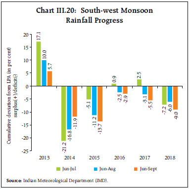 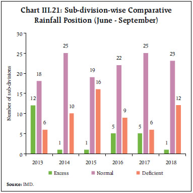 The lower production-weighted rainfall index10 (PRN) for rice, pulses, coarse cereals, oilseeds and cotton in 2018-19 than a year ago may have an adverse impact on eventual production outcomes (Charts III.22 a and b). 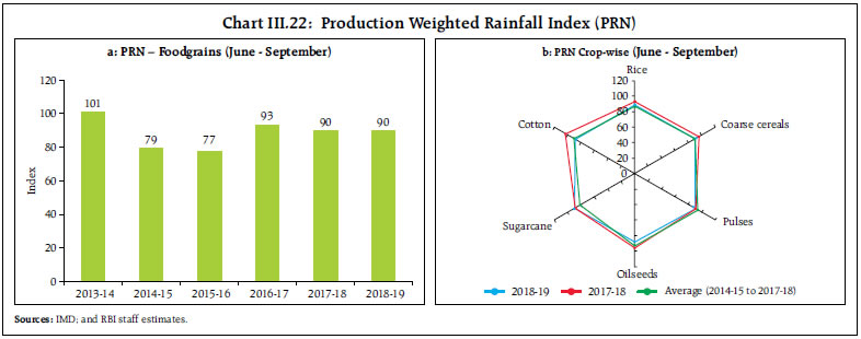 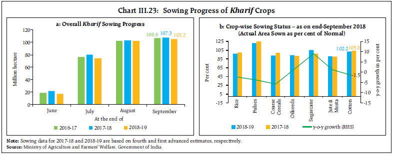 At the commencement of the season, kharif sowing was adversely affected, inter alia, by the delay in the announcement of MSPs, decline in wholesale prices of major food items across mandis on account of bumper harvest and deficient rainfall in major kharif growing states such as Bihar, West Bengal, Jharkhand, Odisha and Uttar Pradesh. However, sowing recovered significantly by end-August with the announcement of MSPs and improvement in precipitation (Charts III.23a and b). The increase in MSP announced for kharif season 2018-19 ensures a return of at least 50 per cent over the cost of production (as measured by A2 plus FL) for all the crops. The highest percentage increase in MSP over the previous year is for ragi (52.5 per cent), followed by jowar hybrid (42.9 per cent), while the lowest increase is for tur (4.1 per cent) and urad (3.7 per cent). Farmers’ sowing decisions might have been influenced more by prevailing wholesale prices rather than the announcement of higher MSPs (Table III.6). For crops such as coarse cereals, pulses and cotton, sowing continues to lag behind in major producing states, despite normal rains – the prevailing wholesale prices for these crops persist below the MSPs. Sowing in oilseeds increased primarily due to farmers shifting away from pulses and cotton in search of higher returns as market prices of oilseeds have remained firm on policy support in the form of import restrictions. Farmers also seem to have switched to soyabean as its wholesale price increased considerably in 2018 so far. Excessive rainfall in Kerala (cumulative rainfall being 23 per cent above LPA by end-September 2018) has adversely affected plantation crops (viz., tea, coffee, rubber, pepper and cardamom) in the state. Heavy rainfalls also impacted plantation of tea, coffee and rubber in Tamil Nadu, cotton crops in 11 districts of Telangana and paddy and cotton crops in Punjab and Haryana. These developments, along with below normal rainfall in Gujarat, Saurashtra and Kutch regions in Central India and the East and North-East parts of the country, may pose downside risks, even if only modest, to the outlook for agriculture. Nevertheless, the first advanced estimates of agricultural production for 2018-19 estimated total kharif foodgrains production at 141.6 million tonnes, 0.6 per cent higher than last year. | Table III.6: Minimum Support Prices for Kharif Season Crops | | Crop | MSP (₹/ Quintal) | Growth Rate (Per cent) | Returns over Cost (A2 plus FL) (Per cent) | | 2016-17 | 2017-18 | 2018-19 | 2018-19 over 2017-18 | 2017-18 over 2016-17 | 2017-18 | 2018-19 | | Paddy common | 1,470 | 1,550 | 1,750 | 12.90 | 5.44 | 38.8 | 50.1 | | Paddy (F)/ Grade ‘A’ | 1,510 | 1,590 | 1,770 | 11.32 | 5.30 | 42.3 | 51.8 | | Jowar-Hybrid | 1,625 | 1,700 | 2,430 | 42.94 | 4.62 | 9.3 | 50.1 | | Jowar-Maldandi | 1,650 | 1,725 | 2,450 | 42.03 | 4.55 | 10.9 | 51.3 | | Bajra | 1,330 | 1,425 | 1,950 | 36.84 | 7.14 | 50.2 | 96.9 | | Ragi | 1,725 | 1,900 | 2,897 | 52.47 | 10.14 | 2.1 | 50.0 | | Maize | 1,365 | 1,425 | 1,700 | 19.30 | 4.40 | 36.5 | 50.3 | | Tur (Arhar) | 5,050 | 5,450 | 5,675 | 4.13 | 7.92 | 64.3 | 65.4 | | Moong | 5,225 | 5,575 | 6,975 | 25.11 | 6.70 | 30.1 | 50.0 | | Urad | 5,000 | 5,400 | 5,600 | 3.70 | 8.00 | 65.4 | 62.9 | | Groundnut | 4,220 | 4,450 | 4,890 | 9.89 | 5.45 | 40.9 | 50.0 | | Sunflower Seed | 3,950 | 4,100 | 5,388 | 31.41 | 3.80 | 17.8 | 50.0 | | Soyabean | 2,775 | 3,050 | 3,399 | 11.44 | 9.91 | 43.8 | 50.0 | | Soyabean Yellow | 2,775 | 3,050 | 3,399 | 11.44 | 9.91 | 43.8 | 50.0 | | Sesamum | 5,000 | 5,300 | 6,249 | 17.91 | 6.00 | 30.3 | 50.0 | | Nigerseed | 3,825 | 4,050 | 5,877 | 45.11 | 5.88 | 3.5 | 50.0 | | Cotton | 3,860 | 4,020 | 5,150 | 28.11 | 4.15 | 22.7 | 50.0 | | Long Staple Cotton | 4,160 | 4,320 | 5,450 | 26.16 | 3.85 | 31.9 | 58.8 | Note: For explanation of A2 plus FL, Chapter II may be referred.
Source: Ministry of Agriculture and Farmers’ Welfare, Government of India. | Live storage in 91 reservoirs was nearly 117 per cent of last year’s storage as on September 27, 2018 and 105 per cent of the decennial average, which augurs well for the coming rabi sowing season. Lower storage in western regions will, however, need to be monitored, going forward. III.2.2 Industry Industrial production turned broad-based during April-July, benefitting from base effect (Chart III.24a). Expansion of output occurred in 20 out of 23 manufacturing industry groups in July 2018. Petroleum products, motor vehicles, computer and electronic equipments, basic metals and other non-metalic mineral products emerged as key drivers during April-July 2018 (Chart III.24b). The index of eight core industries (40.3 per cent weight in IIP) for April-August 2018 also shows healthy growth. Electricity generation also gathered steam and supported industrial activity. A rise in power demand, especially from DISCOMs, coinciding with temporary shortfalls in the supply of energy from renewable sources, pushed up the demand for thermal power (Chart III.25). In response, shortages of coal in power plants are being addressed through improved supplies from Coal India Ltd., which has reduced the power deficit. The sustained firming up of manufacturing activity was also reflected in the robust growth in nominal sales and profits before tax of listed non-government manufacturing companies in 2017-18 (Chart III.26). An analysis of 1,741 listed companies for Q1:2018- 19 also attests to improvement in profitability of manufacturing firms (Chart III.27). Based on the use-based classification, industrial production was driven by sustained acceleration in primary goods, infrastructure/construction goods, capital goods and consumer durables in Q1:2018-19 (Chart III.28). Increased production of diesel, LPG, fertilisers, mining produce and electricity helped push up the supply of primary goods. The production of steel and cement remained buoyant, underpinned by public sector infrastructure projects, including affordable housing, and a pick-up in sales and new launches of residential units. Consumer durables production is being buoyed by strong urban demand. 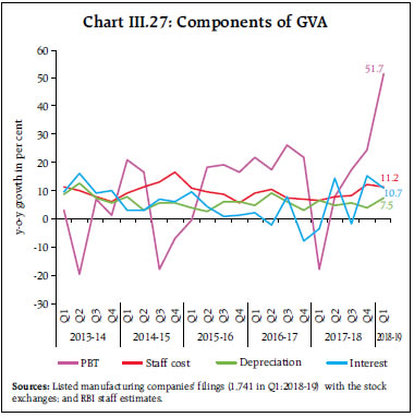 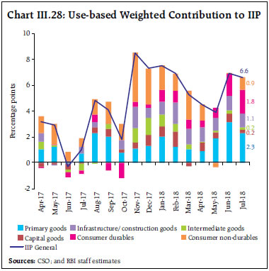 Overall business sentiment in the Indian manufacturing sector has remained broadly stable. The expectations based on business expectations index (BEI) improved to 115.0 for Q3:2018-19 (from 114.1 in Q2) in the 83rd round of the Reserve Bank’s Industrial Outlook Survey (IOS), primarily driven by order books. The early indicators of assessment for Q2:2018-19 also point to optimism on demand conditions. The manufacturing purchasing managers’ index (PMI) expanded for the fourteenth consecutive month in September, supported by higher levels of output, employment and new orders. III.2.3 Services Services sector activity moderated sequentially in Q1:2018-19. On the whole, however, services sector growth has remained resilient, supported by construction activity and PADO. A pick-up in real estate activity and bank credit reinforced activity in financial, real estate and professional services. In the transportation sub-sector, passenger traffic by rail and air moderated in Q1:2018-19 (Chart III.29a). Cargo transport indicators, however, accelerated (Chart III.29b). The services PMI moderated in August-September 2018 after touching a 21-month high in July (54.2). The production of cement and consumption of steel – key indicators of construction activity – remained upbeat in April-August 2018 (Chart III.30), benefiting from robust domestic demand in the infrastructure and construction sectors, in part, due to the impetus from the Pradhan Mantri Awas Yojana (PMAY). A moderation in domestic steel prices is likely to strengthen steel consumption going forward. 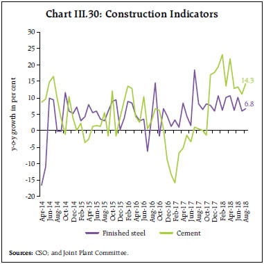 PADO growth moderated, reflecting subdued revenue expenditure (net of interest payments and subsidies) of the Union Government. The growth of financial, real estate and professional services accelerated sequentially in Q1:2018-19, underpinned by steady acceleration of bank credit and deposit growth (Chart III.31). Real estate activity seems to be recovering as the number of housing units launched and sales both improved sequentially in Q1:2018-19 (Chart III.32a). Nevertheless, the overhang of unsold inventory and weaker demand conditions continued to have a moderating influence on residential home prices (Chart III.32b). III.3 Output Gap Potential output tends to be driven by the supply of labour and capital and the growth of total factor productivity (TFP).11 Productivity is a key determinant of potential output. The KLEMS12 database suggests that TFP growth in various sub-sectors of industry and services, with relatively higher contributions to overall GVA in the Indian economy, has improved in the post-global financial crisis period, i.e., 2010-11 to 2015-16, vis-à-vis 2004-05 to 2009-10 (Chart III.33). Output gap estimates (i.e., the deviation of actual output from its potential level expressed as ratio of potential output) provide a summary indicator of demand-supply conditions. Both potential output and the output gap are unobservable and their estimates can be sensitive to the method of estimation. Hence, a variety of alternative approaches – univariate filters such as the Hodrick-Prescott filter; the Baxter-King filter; the Christiano-Fitzgerald filter; and multivariate Kalman filters (MVKF), which can take into account inflation or financial conditions, have been employed for drawing robust inferences on the stage of the business cycle.13 The composite estimate of the output gap, obtained by using principal components analysis on the alternative estimates, suggests that the output gap has virtually closed in Q1:2018- 19 (Chart III.34a). It reflects the acceleration in the pace of domestic demand from the second quarter of 2017-18, with real GDP growth increasing from 5.6 per cent in Q1:2017-18 to 8.2 per cent in Q1:2018-19. 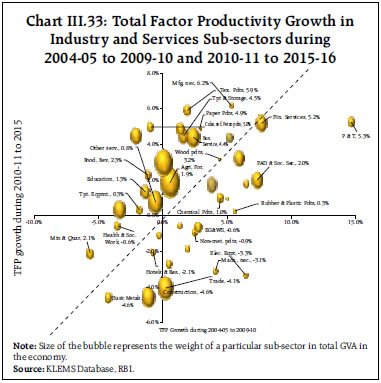 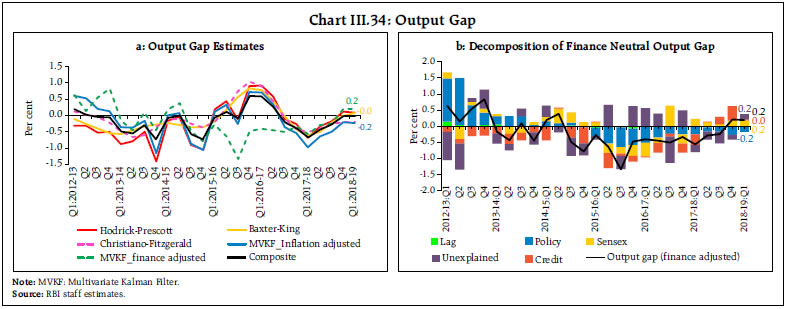 The output gap dynamics are also consistent with the uptick in capacity utilisation (seasonally adjusted) in the manufacturing sector. The finance-adjusted output gap remained marginally positive in Q1:2018-19, driven by growth in overall credit and equity prices (Chart III.34b). III.4 Conclusion The recovery in economic activity, which began in Q2:2017-18, seems to be robust. Consumption is expected to remain resilient, buoyed by rising income levels and staggered implementation of the 7th Central Pay Commission (CPC) award at the states’ level in the urban areas. Rural consumption is likely to remain strong in view of the sizeable hike in MSPs and debt waivers by the states. The record agricultural production achieved in recent years, is expected to be maintained on the back of a hike in MSPs of kharif crops, normal monsoon rains in most of the kharif crop growing regions of the country and comfortable water reservoir storage. Easier supply conditions in the agrarian economy support backward and forward linkages and thereby brighten the prospects for the manufacturing and services sectors. Upbeat construction activity, fading away of the slack in banking sector financial intermediation activities, and higher public expenditure in an election year, suggest that stability of services sector growth would be maintained. A more durable momentum in investment activity holds the key to sustaining the Indian economy on the higher growth path that has become evident in the last two quarters. Rising capacity utilisation and improving credit offtake bode well for investment gaining traction. The deteriorating global trade and geo-political environment are, however, negative risks to the investment outlook.
IV. Financial Markets and Liquidity Conditions Domestic financial market segments exhibited divergent movements in the first half of 2018-19. Money markets experienced liquidity swings while the government securities and foreign exchange market segments were impacted by global spillovers. The stock market scaled new highs on buying support from domestic mutual funds. In the credit market, bank lending gained traction amidst some tightening of financing conditions. Global financial markets were unsettled during the first half of the year by bouts of turbulence stirred up by the collision of the ongoing normalisation of monetary policy, elevated and volatile crude oil prices, geopolitical tensions and country-specific stresses. While equity markets in advanced economies (AEs) remained buoyant and undeterred by rising interest rates in the United States (US), yield curves in bond markets continued to flatten as term spreads declined. The US dollar strengthened persistently up to mid- August, leading to across-the-board depreciation of the currencies of emerging market economies (EMEs), with marked declines in some of them. As investors turned risk-averse towards EMEs as an asset class, capital outflows became pronounced, leading to corrections in their equity markets, hardening of bond yields, and increase in credit spreads. For some EMEs, country-specific factors accentuated the decline in asset prices and exodus of capital flows. Different segments of the domestic financial market were impacted divergently by global spillovers and local developments. Overnight money markets remained immune and interest rates traded below the policy repo rate, notwithstanding oscillating liquidity conditions and two policy rate hikes in June and August. Interest rates on Treasury Bills (T-Bills), on the other hand, hardened synchronously with the spectrum of gilt yields up to the longer end, reflecting both global developments and perceptions of an oversupply of government paper. Yields on corporate bonds tracked those on government bonds. Equity markets were driven by rallies to new highs as ebullient domestic institutional investors more than compensated the sell-off by foreign portfolio investors (FPIs), though there have been recent signs of a broad-based correction. The exchange rate of the rupee came under sporadic bouts of pressure due to capital outflows by FPIs and widening of the trade deficit. Overall, the depreciation of the Indian Rupee (INR) was “middle of the pack” in comparison with EME currency peers. Credit flows from banks gathered momentum and became broad-based even as several banks increased their lending rates to reflect the strengthening demand for bank credit and moderation of surplus liquidity in the system. IV.1 Financial Markets As alluded to above, there was a marked differentiation in the drivers of activity in the various constituents of the domestic financial market continuum. While the foreign exchange and bond segments were affected by the adverse mix of global developments, equity markets were a notable outlier, cushioned by domestic bullishness. Likewise, the money and credit markets were unaffected by global factors, the former insulated by persisting albeit shrinking systemic surplus liquidity and the latter by a steady revival of domestic demand. IV.1.1 Money Market: Systemic liquidity underwent alternating phases in H1:2018-19. Substantial surpluses in April and May gave way to deficits for a brief period from mid-June to July 2018 due to advance tax outflows and forex operations of the Reserve Bank. Surplus conditions returned, however, in the first half of August due to increase in government spending, although from August 21 onwards, indirect tax payments whittled down excess liquidity for a brief period. Surplus conditions returned in the first ten days of September before tightening in the second half on account of advance tax outflows. Average daily net liquidity absorbed through the liquidity adjustment facility (LAF) turned from ₹496 billion in April to a net injection of ₹107 billion in July before switching back into net absorption of ₹30 billion in August. The liquidity deficit in the second half of September resulted in daily net injection of liquidity throught the LAF to the tune of ₹406 billion. The weighted average call rate (WACR) traded generally below the policy repo rate (Chart IV.1). 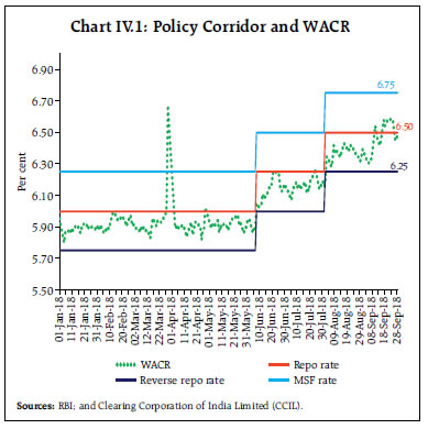 The negative spread of the WACR over the repo rate increased from 11 bps in April to 15 bps in August (notwithstanding some intermittent moderation in May and July) before moderating to 4 bps in September. Overall, the WACR, on average, remained 10 bps below the policy rate in H1: 2018-19 (Chart IV.2). In money markets, both rates and volumes have adjusted to institutional and policy changes introduced by the Reserve Bank of India (RBI). For instance, the width of the policy corridor, which was 200 bps in May 2011, was progressively reduced to 50 bps by April 2017 as a part of ongoing refinements of the operating procedure of monetary policy. Empirical research and international evidence suggest that the width of the corridor is positively related to volatility – a wider corridor is associated with higher volatility in the inter-bank market and vice versa (Bindseil and Jablecki, 2011).1 In India, the narrowing of the corridor has moderated volatility – measured by the exponential weighted moving average (EWMA) of the inter-bank call rate – significantly, corroborating the cross-country experience (Chart IV.3).2 This has, however, not produced any significant adverse impact on volumes in the uncollateralised segment – the share of the call money market in the total inter-bank overnight market turnover remained broadly unchanged at less than 10 per cent (Chart IV.4). 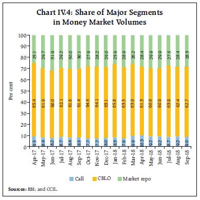 In terms of market microstructure, private banks and primary dealers (PDs) are the major borrowers in the overnight call money market, while co-operative banks and public sector banks are the major lenders. In the collateralised borrowing and lending obligations (CBLO) segment (which constitutes more than 60 per cent of the overnight market), banks are usually borrowers, while mutual funds (MFs) are major lenders. The share of MFs in CBLO lending, which had gone up to 80 per cent in March 2017 in the wake of demonetisation, gradually ebbed and stabilised at an average share of 64 per cent in H1:2018-19. In the collateralised market repo segment (which constitutes about 30 per cent of the overall overnight market turnover), MFs are major lenders, followed by foreign banks. On the other hand, PDs are the largest borrowers in this market, followed by foreign banks. During H1:2018-19, interest rates in both the collateralised segments, i.e., CBLO and market repo were, on an average, below the WACR by ten bps and three bps, respectively (Chart IV.5). 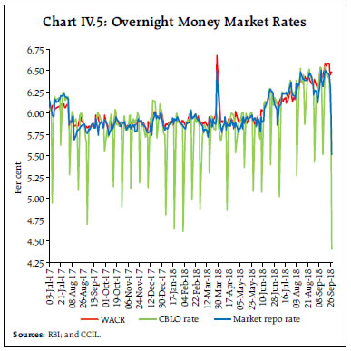 Turnover in the three overnight segments undergoes marked intra-day variations. Foreign banks and PDs – major borrowers in the market repo segment – meet around 80 per cent of their funding requirements for government securities (G-sec) trades during the first hour i.e., 9:00-10:00 am, even though the market is open up to 2:30 pm (T+0 settlement). The concentration of trading activity in the first hour implies thin trading for the rest of the day, which increases intra-day volatility and spillovers on to other overnight market segments. Transactions of MFs in the CBLO segment are allowed to be routed through designated banks within banking hours (generally up to 2.30 pm) in order to provide adequate time for settlement at designated settlement banks; trading becomes thin thereafter. Consequently, demand spills over to the uncollateralised call money segment – the only active segment in late trading hours – often resulting in spikes in call rates. Overnight interest rates in all the three segments trade at elevated levels in the early hours as most market participants rush to bridge liquidity mismatches. Competitive trading in the morning hours narrows interest rate differentials across segments (Chart IV.6a). Volatility in call and the CBLO rates is also the lowest in the early hours (Chart IV.6b). Subsequently, as volumes dip and volatility rises, interest rates decline, though at different speeds, reflecting segment-specific factors. For instance, activity in the call money market in the afternoon is largely driven by co-operative banks, which typically lend at lower rates than the prevailing call rate, leading to higher volatility. 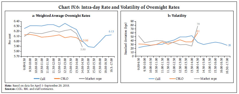 Interest rates on longer tenor money market instruments such as certificates of deposit (CDs), commercial papers (CPs) and 91-day Treasury Bills (T-Bills) moved disparately during H1:2018-19. Interest rates on CDs (3-month maturity) moderated at the beginning of April due to liquidity conditions turning into surplus with the unwinding of large government cash balances. However, they hardened until the first week of June, i.e., from 6.80 per cent at end-March 2018 to 7.91 per cent as on June 5, 2018 (Chart IV.7). In its June policy announcement, when the RBI provided a deeper carve-out from the statutory liquidity ratio (SLR) to meet the liquidity coverage ratio (LCR), 3-month CD rates softened by about 37 bps as banks’ requirements of bulk deposits waned. As surplus liquidity shrank in June and turned into deficit in July, fresh issuances of CDs also increased to ₹1,988 billion during H1 (up to September 14, 2018) – as compared with ₹1,420 billion in H1:2017-18 – accompanied by higher rates. After the policy rate hike in August 2018, the 3-month CD rate inched up by about 10 bps. Movements in CP rates were similar, but they traded above the CD rates due to strong appetite for CPs as credit substitutes in non-financial corporations for working capital needs, in view of the relatively costlier bank loans, and as a way of keeping marginal funding costs low in non-bank financial companies. Amount of CP issuance surged and interest rates on CPs hardened through H1:2018-19. In particular, issuances of CPs increased from ₹9,316 billion in H1:2017-18 to ₹12,456 billion in H1:2018-19 (up to September 15, 2018). After the June policy announcement, 3-month CP rates declined by about 30 bps tracking the decline in CD rates. Similarly, the 3-month CP rate declined by about 15 bps after the August policy announcement (Chart IV.7). The 91-day T-Bill rate was elevated through Q1 and following the increase in the policy rate in June, it edged up by two bps. After the rate hike in August 2018, it inched up further by about four bps. The Infrastructure Leasing and Financial Services Limited (IL&FS), which is a systemically important non-deposit accepting core investment company (CIC-ND-SI) registered with the Reserve Bank of India, is currently owned by various institutional shareholders, including Life Insurance Corporation of India (LIC), ORIX Corporation Japan, Abu Dhabi Investment Authority, IL&FS Employees Welfare Trust, Housing Development Finance Corporation, Central Bank of India and State Bank of India. The company has witnessed a series of rating downgrades since August 2018 and a succession of defaults on its CPs, non-convertible debentures (NCDs) and bank loans. Consequent to the default by IL&FS on its obligations on September 14, 2018, the weighted average discount rate on CPs increased in general, and that for non banking financial companies (NBFCs), in particular. In the secondary CP market, the 3-month CP rate jumped from around 7.8 per cent at the beginning of September to 8.15 per cent on September 21, 2018, triggered also by sales of NCDs at steep discounts by an individual mutual fund on September 21, 2018, and further to 9.0 per cent on September 26, 2018. The RBI and the Securities and Exchange Board of India (SEBI) issued press releases on September 23, 2018 indicating that they are closely monitoring recent developments in financial markets and are ready to take appropriate actions, if necessary. Yields softened by 40 bps by end-September. Based on the assessment of prevailing liquidity conditions, liquidity needs going forward and the expansion in currency in circulation, the RBI has taken several measures to inject liquidity into the system in the second-half of September (Box IV.1). | Box IV.1: Policy Measures by the Reserve Bank of India since mid-September 2018 | | Date /Month | Liquidity Measures | | September 19 and 27, 2018 | The RBI conducted two back-to-back open market operation (OMO) purchase of government securities for an aggregate amount of ₹100 billion each on September 19 and September 27, 2018. | | September 2018 | The RBI conducted several variable rate repo of longer tenors under the LAF during September 2018 in addition to the regular 14-day variable rate repos in order to provide a liberal infusion of liquidity. | | September 27, 2018 | The RBI decided to permit banks with effect from October 1, 2018, to reckon government securities held by them up to another 2 per cent of their net demand and time liabilities (NDTL), under the facility to avail liquidity for liquidity coverage ratio (FALLCR) within the mandatory SLR requirement, as Level 1 high-quality liquid assets (HQLA) for computing their LCR. Hence, the carve-out from SLR, under FALLCR will now be 13 per cent, taking the total carve out from SLR available to banks to 15 per cent of their NDTL. The RBI clarified that there was ample liquidity surplus in the system and that, going forward, it would stand ready to meet the durable liquidity requirements of the system through various available instruments depending on its dynamic assessment of the evolving liquidity and market conditions. | | October 01, 2018 | The RBI decided to conduct purchase of government securities under OMOs for an aggregate amount of ₹360 billion in the month of October 2018. The auctions would be conducted during the 2nd, 3rd and 4th week of October. The RBI retains the flexibility to change the amount, depending on the evolving liquidity and market conditions. |
IV.1.2 Government Securities (G-sec) Market: G-sec yields eased at the beginning of 2018-19, with market sentiment buoyed by several positive developments, viz., (i) announcement of reduced market borrowings in the Union Budget along with the decision by the central government not to front load issuances in the first half of 2018-19; (ii) the RBI allowing banks to spread out mark-to-market (MTM) losses incurred during Q3:2017-18 and Q4 of 2017-18, over four ensuing quarters; (iii) no change in the repo rate by the Monetary Policy Committee (MPC) in the April 2018 policy; and (iv) a downward revision in the inflation forecast for H1:2018-19. The softening of yields by 16 bps, however, proved transitory and they hardened by 44 bps in end-April on account of several factors such as (i) the release of larger than expected borrowing calendar for state development loans (SDL); (ii) rising international crude oil prices; (iii) inflation concerns due to the revised formula for minimum support price (MSP) as announced in the Union Budget 2018-19; (iv) depreciation of the rupee; (v) rising trade protectionism; and (vi) MPC minutes which flagged upside risks to inflation. Yields softened by 19 bps in the first week of May after the announcement of OMOs by the RBI and the decision to lift the three-year maturity cap on foreign portfolio investment (FPI) along with an increase in the overall FPI limit. Yields hardened again, however, by 31 bps in the remaining part of May on account of several factors such as (i) the firming up of US treasury yields to 3.0 per cent (first time since January 2014); (ii) the unrelenting rise in global crude oil prices breaking through the three and a half year peak; (iii) a higher than expected April CPI inflation print; and (iv) concerns on the pace of US Fed rate hikes. In June, the sentiment was initially boosted by higher than expected gross domestic product (GDP) growth in the January-March print. Thereafter, G-sec yields increased in sync with the repo rate hike of 25 bps. Bearishness set in on rising global crude oil prices and a depreciating Indian Rupee (INR), which posed risks to the domestic inflation outlook. The benchmark 10-year G-sec yield closed at 7.90 per cent on June 29, 2018, with overall benchmark yields rising by 57 bps during Q1:2018-19. The G-sec market traded with a softening bias up to August 21, 2018, reflecting the easing of crude oil prices on expectation of increased supplies, lower than expected June inflation print and the announcement of OMO purchases. Yields, however, hardened in end-August tracking the rebound in crude oil prices and depreciation of the INR. The 10-year benchmark yield fell to 7.77 per cent in July and moderated further in the first week of August, driven down by a decline in crude prices. Notably, the 10-year benchmark yield fell by seven bps on August 1 on positive global cues, despite the rate hike by the RBI on the same day. In sync with the depreciation of the INR, however, yields peaked to a high of 8.11 per cent on September 11, 2018. Despite high volatility witnessed during the month which tracked the movements in crude oil prices and INR, yields softened towards the month end and closed at 8 per cent on September 28, 2018, reflecting the measures taken for containing INR volatility along with expectations of lower market borrowings by the central government in H2:2018-19 (Chart IV.8). 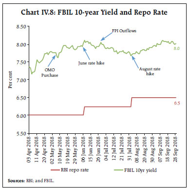 The yield curve has undergone level shifts in H1:2018-19 in response to global spillovers as well as domestic factors such as near-term inflation outlook and monetary policy measures (Chart IV.9). The rate hike of June resulted in a parallel upward shift in the yield curve, especially in the 2-year to 16-year segment, while the August rate hike induced a downward shift, in line with softening crude oil prices. FPIs remained net sellers in the G-sec market during the most part of H1:2018-19, but turned net buyers in July and August (Chart IV.10). FPIs made net sales of ₹274.17 billion in the G-sec segment, including ₹30.88 billion in state development loans (SDLs). At the shorter end of the primary market segment, yields on treasury bills tracked the benchmark 10-year G-sec yield and hardened during H1, also reflecting the increase in the policy rate by 25 bps each in June and August, concerns on liquidity, and depreciation pressure on the INR (Chart IV.11). At the longer end, the issuance of SDLs was moderate during H1:2018-19. State government market borrowings, however, are expected to go up in H2 due to redemption pressure arising out of past issuances. The weighted average spread of SDLs’ cut-off over the corresponding tenor G-sec yield moderated to 53 bps in H1:2018-19 from 63 bps in H1:2017-18 (Chart IV.12). The average inter-state spread on securities of 10-year tenor during H1:2018- 19 was at four bps, lower than nine bps in H1:2017- 18. The maximum inter-state spread peaked at 23 bps on April 10, 2018. 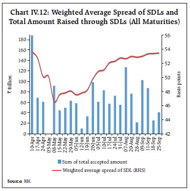 IV.1.3 Corporate Bond Market: Corporate bond yields have largely tracked G-sec yields (Chart IV.13a). Interest rates on AAA 5-year corporate bonds hardened significantly by 81 basis points to 8.78 per cent in Q1: 2018-19 and further by 8 basis points to 8.86 per cent in Q2. The yield spread of 5-year AAA corporate bonds over 5-year G-secs increased sharply by 21 basis points during H1:2018-19, reflecting perceptions of heightened credit risk, which was also corroborated by higher credit default swap (CDS) spreads on State Bank of India and ICICI Bank papers in an environment of rising global uncertainty. 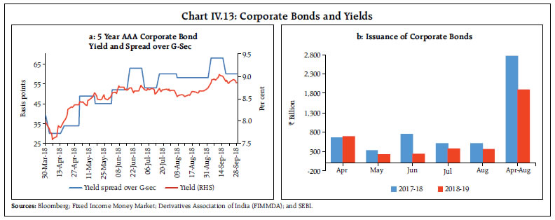 Average daily turnover in the corporate bond market declined marginally to ₹71.3 billion during H1:2018- 19 from ₹73.0 billion during the corresponding period of the previous year. The surge in bond yields induced corporates to shift to bank credit for meeting their funding requirements. Consequently, resource mobilisation through issuances of corporate bonds in the primary market declined by 31.3 per cent to ₹1,906 billion during April-August 2018 from ₹2,773 billion during the corresponding period of the previous year (Chart IV.13b). The bulk of resource mobilisation continued to favour the private placement route – 89 per cent of the total mobilisation from the corporate bond market. Investments by FPIs in corporate bonds declined to ₹2.01 trillion at end-September 2018 from ₹2.24 trillion at end-March 2018. Consequently, FPIs’ utilisation of the approved limit for investment in corporate bonds declined sharply to 75.5 per cent at end-September 2018 from 91.9 per cent at end-March 2018. IV.1.4 Stock Market: Exuberance marked the movements in the equity market during the first five months of H1:2018-19, with the BSE Sensex rising sharply to touch a high of 38,897 at close on August 28, 2018 before moderating to 36,227 at end-September 2018, but still registering an increase of 9.9 per cent during H1:2018-19. The Indian equity market generally remained resilient in the face of sell-offs in many emerging market (EM) stocks, with the MSCI-EME index3 declining by 10.5 per cent during the period. The price earnings (P/E) ratio of Indian equity, which is an indicator of stock market valuation, has generally remained above the P/E ratios of other EM and AE stocks, indicating that investors are willing to pay a higher price for Indian stocks on higher growth expectations or anticipation of continued domestic inflows into mutual fund investments in equities. The P/E ratio of Sensex increased to 23.7 at end-September 2018 from 22.5 at end-March 2018, which was in sharp contrast to a decline in the P/E ratio in the case of other EM indices (Chart IV.14a and b). 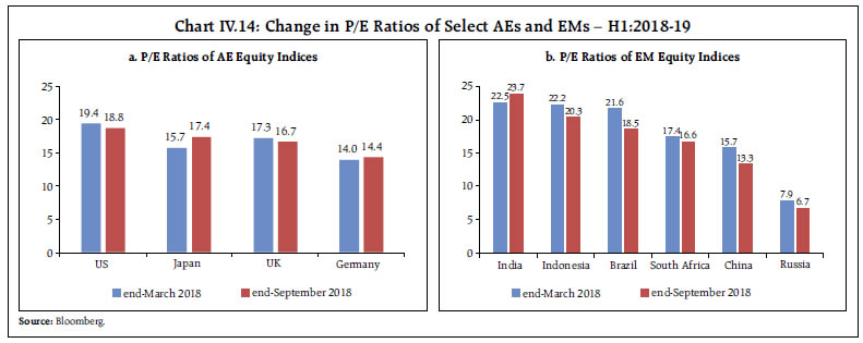 The rally in the Indian equity market till mid-July 2018 was primarily restricted to stocks of a few blue-chip companies. This was indicative of investors’ preference for quality stocks in times of heightened global uncertainty. During the period mid-July 2018 to end-August 2018, however, the rally in the equity market became more broad-based, indicative of the widening of buying interest. The equity market witnessed significant correction in September 2018 with the broader indices, viz., BSE MidCap and BSE SmallCap, declining more sharply than the BSE Sensex. Overall, the BSE MidCap index and the BSE SmallCap index declined by 7.5 per cent and 15.1 per cent, respectively, during H1:2018-19. After a sharp correction during February and March 2018, market sentiment turned positive in Q1:2018- 19, with the BSE Sensex increasing sharply by 7.4 per cent, mainly on account of a lower-than-expected market borrowing programme of the Centre for H1:2018-19, better than expected corporate earnings performance in Q4:2017-18, positive economic news releases such as buoyant goods and services tax (GST) collections and higher auto sales, and sustained buying by MFs. The sharp rally in April was followed by some correction in the second half of May 2018 on uncertainty relating to the election outcome in Karnataka and trade war concerns. The market moved sideways in June 2018 on continuing trade frictions, surge in crude oil prices and interest rate hike by the US Fed on June 13, 2018, along with indications of two more hikes by the end of 2018 (Chart IV.15a). 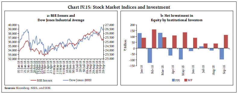 After this brief interlude, the rally in the equity market resumed during the first two months of Q2: 2018-19 with the BSE Sensex increasing sharply by 9.1 per cent during July-August 2018, mainly on the back of domestic factors such as better corporate earnings results for Q1:2018-19, Government’s approval of capital infusion into five public sector banks, reduction in GST rates on several items, better than expected GDP growth for Q1:2018-19 and decline in inflation in July and August. While the market underwent some decline in the second week of August mainly on concerns about potential market contagion from the crisis in Turkey, it recovered later in the month, especially after the US Fed Chairman’s speech that reaffirmed a gradual approach to interest rate hikes. During September 2018, however, the market registered significant losses with the BSE Sensex declining by 2418 points (6.3 per cent), triggered by default on its debt obligations by IL&FS, which raised concerns about liquidity shortage in the NBFCs sector. Additionally, lingering concerns relating to trade war between the US and China and sharp depreciation of the INR against the US dollar, in the backdrop of higher oil prices and widening of India’s current account deficit for Q1:2018-19, exacerbated the fall in the equity market. Overall, during Q2:2018-19, the BSE Sensex registered a modest increase of 2.3 per cent. During H1:2018-19, domestic institutional investors, particularly MFs, made net purchases of ₹529 billion in the equity market, while FPIs made net sales of ₹287 billion (Chart IV.15b). In the primary segment of the equity market, resource mobilisation through public issues of equity (initial public offers and right issues) increased by 7.9 per cent to ₹120.3 billion during April-August 2018 as compared with ₹111.5 billion in the corresponding period of the previous year. IV.1.5 Foreign Exchange Market: Since April 2018, the INR traded with a depreciating bias, dipping to a low of ₹72.81 per US dollar (reference rate) on September 25, 2018. The fall in the INR, however, was no exception as currencies of EMEs – both current account deficit and surplus countries – lost value as the US dollar strengthened during this period. In particular, sell-offs by FPIs, the ongoing monetary policy normalisation by the US Fed, and country-specific factors – China recorded its first quarterly current account deficit in Q1:2018 after 17 years – drove many EME currencies into depreciation in Q1:2018-19. Subsequently, as concerns over the sell-off in Turkish lira exacerbated in August, several EME currencies plunged to multi-year lows. Global risks for EME currencies also seem to be shifting back to China, boosting safe-haven demand for the US dollar amidst escalating concerns of trade frictions between the US and China. While the INR depreciated by 10.3 per cent vis-a-vis the US dollar between end-March and end-September 2018, it was modest in comparison with the depreciation of the Brazilian Real, the South African Rand, the Turkish Lira, the Argentine Peso and the Russian Ruble (Chart IV.16a). The size of depreciation of EME currencies, including the INR, in real effective terms was far modest than in nominal terms (Chart IV.16b). In terms of both the nominal effective exchange rate (NEER) and the real effective exchange rate (REER), the rupee depreciated by 5.6 per cent and 5.0 per cent, respectively, between March (average) and September 28, 2018 (Chart IV.16b and Table IV.1). | Table IV.1: Nominal and Real Effective Exchange Rates – Trade-based | | (Base: 2004-05 = 100) | | Item | Index: September 28, 2018 (P) | Appreciation (+) / Depreciation (-) (Per cent) | | September 28, 2018 over March 2018 | March 2018 over March 2017 | | 36-currency REER | 111 | -5.0 | -0.8 | | 36-currency NEER | 71 | -5.6 | -2.9 | | 6-currency REER | 119 | -4.7 | -3.8 | | 6-currency NEER | 61 | -6.0 | -6.0 | | ₹/ US$ (As on September 28, 2018) | 73 | -10.4 | 1.3 | P: Provisional.
Note: REER figures are based on the Consumer Price Index (Combined).
Source: RBI. | In the recent period, uncertainty around certain global factors has triggered episodic bouts of volatility in both the G-sec and forex markets in India (Box IV.2). IV.1.6 Credit Market: In the credit market, non-food credit growth accelerated to reach its highest level of the last four years in August 2018 (13.5 per cent), with the momentum offsetting generally unfavorable base effects (Chart IV.17). As of September 14, 2018, non-food credit growth was placed at 12.5 per cent. Credit extended by public sector and foreign banks has been recovering gradually and this was built upon during H1:2018-19 (Chart IV.18). Of the incremental credit extended by scheduled commercial banks as of September 2018, 57.3 per cent was provided by public sector banks and 4.1 per cent by foreign banks, which was 29.3 per cent higher and 4.1 per cent, lower respectively, a year ago. Box IV.2: Bond and Forex Markets in Uncertain Times In India, the G-sec and forex markets have turned volatile in recent months, hit by global spillovers that destabilised market sentiments and led to episodic bouts of market volatility (Chart IV.2.1). Following Belke et al. (2016), the impact of uncertainty on market movements has been empirically examined with daily and monthly data for the period January 1, 2009 to July 31, 2018. In the absence of any definitive measure of day-to-day uncertainty, the India VIX, based on NIFTY index option prices, has been used as a proxy (RBI, 2018). A preliminary analysis showed evidence of volatility clustering in yields and exchange rates. The generalised autoregressive conditional heteroscedasticity (GARCH) model was estimated, which allows conditional variance to depend on its lagged values. In the GARCH (1,1) specification, the mean equation indicates the magnitude and direction of impact of the explanatory variables (one period lagged value of change in G-sec yields or percentage returns on daily exchange rates, log of India VIX index and its lags) on the dependent variable (change in G-sec yields or percentage returns on daily exchange rate). The conditional variance equation helps identify time-varying volatility of the residuals generated from the mean equation. Accordingly, the following GARCH(1,1) mean and volatility equations were specified: where, Depvart is the change in daily 10-year G-sec yield or percentage returns on daily exchange rates and VIX capturing uncertainty which is reflected in day-to-day volatility. Based on daily data, GARCH(1,1) estimates using changes in daily 10-year G-sec yield (ΔYLD10YR), percentage returns on daily exchange rates (%CEXR) and day-to-day volatility (LVIX) reveal interesting insights. The mean equation suggests that an increase in uncertainty causes hardening of yields and a depreciation of the INR (Table IV.2.1). The sum of α and β coefficients in the variance equation is less than unity, implying that the model is stable. | Table IV.2.1. Results from GARCH(1,1) Model | | | ΔYLD10YR | %CEXR | | Mean Equations | | | | Depvart-1 | 0.010 (0.57) | -0.078 (0.00) | | LVIXt | 0.023 (0.06) | 1.028 (0.00) | | LVIXt-1 | -0.021 (0.07) | – | | LVIXt-2 | – | -1.021 (0.00) | | C | -0.004 (0.36) | -0.006 (0.90) | | Variance Equations | | | | C | 0.000 (0.00) | 0.001 (0.00) | | α | 0.029 (0.00) | 0.040 (0.00) | | β | 0.964 (0.00) | 0.956 (0.00) | | Diagnostics | | | | ARCH test (p-value) | 0.92 | 0.17 | | Note: Figures in parentheses are respective p-values. | In order to test the impact of uncertainty on G-sec yields and the INR-USD on a monthly frequency, the economic policy uncertainty index4 for India, based on the methodology of Baker et al. (2015) and available from the Federal Reserve Bank of St. Louis was used (Chart IV.2.2). To test the hypothesis of uncertainty impacting the domestic bond and forex markets, a pair-wise co-integrated vector auto-regression (VAR) model was used after checking for stationarity properties of the variables (with logarithmic transformation of all the series, excepting the G-sec yield) for the period January 2009 – July 2018. 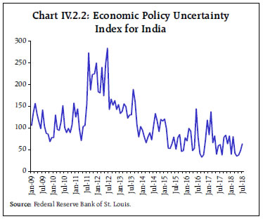 Data were found to be non-stationary in levels but stationary in first differences in the Augmented Dickey- Fuller (ADF) tests. Johansen’s cointegration method revealed existence of pair-wise long-run relationships, viz., (i) between the yield on 10-year G-sec (YLD) and the policy uncertainty index (LPUI); and (ii) between the INR-USD (LEXR) and the policy uncertainty index (LPUI), as indicated below: YLD = 0.27 + 1.63*LPUI ……. (1); and
LEXR = -0.21 + 0.47*LPUI …. (2) These results suggest that the G-Sec yield increases by 16 basis points and INR-USD depreciates by 4.7 per cent for every 10 per cent increase in the policy uncertainty index (LPUI). In order to examine the short-run dynamic relationship, vector error correction models (VECMs) were estimated. The error correction terms for both the explanatory variables have statistically significant negative signs, implying that the underlying mechanisms are convergent and, therefore, correct for disequilibrium. Furthermore, to test the direction of causality, the Granger causality or Block Exogeneity Wald tests based on the VECM were carried out. The null hypothesis that policy uncertainty does not Granger cause 10-year G-sec yield was rejected (at 5 per cent level of significance), while the reverse causality was ruled out, indicating that policy uncertainty uni-directionally causes changes in the G-sec yield. Similar, uni-directional causality was also observed for policy uncertainty to INR-USD (Table IV.2.2). These findings suggest that the impact of policy uncertainty is significant on G-sec yields and INR-USD, both at daily and monthly frequencies, as evident in recent episodes of market volatility. References: Belke, A., I. Dubova and T. Osowski (2016), “Policy Uncertainty and International Financial Markets: The Case of Brexit”, CEPS Working Document No. 429 / November. Baker, S. R., N. Bloom and S. J. Davis (2015), “Measuring Economic Policy Uncertainty”, NBER Working Paper 21633, October. RBI (2018), Annual Report, 2017-18, August. | Table IV.2.2: VEC Granger Causality/Block Exogeneity Wald Tests | | Dependent variable: ΔYLD | Dependent variable: ΔLPUI | | | Chi-Sq | df | Prob | | Chi-Sq | df | Prob | | ΔLPUI | 5.90 | 1 | 0.02 | ΔYLD | 0.97 | 1 | 0.32 | | Dependent variable: ΔLEXR | Dependent variable: ΔLPUI | | | Chi-Sq | df | Prob | | Chi-Sq | df | Prob | | ΔLPUI | 4.00 | 1 | 0.04 | ΔLEXR | 0.60 | 1 | 0.44 | | Note: Chi-Sq: Chi-square statistic; df: degrees of freedom; Prob: Probability value. | |
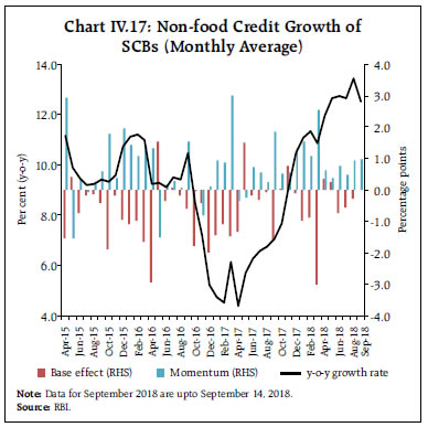 Incremental credit flow is also getting increasingly diversified, with services accounting for the highest share (as of July 2018) as against personal loans a year ago (Chart IV.19). Credit growth to industry, which has been positive since November 2017, after more than a year-long contraction, showed significantly improved flows to textiles, mining and quarrying, engineering, and telecommunications. The share of credit to agriculture, however, moderated, which might be indicative of pressures in the farm sector as corroborated by agriculture debt waivers announced in some states.
While the overall non-performing assets (NPA) ratio of SCBs moderated in June when compared with end- March 2018, it deteriorated in the case of personal loans and agriculture – the sectors that received large credit flows in recent years (Chart IV.20a). In contrast, the NPA ratio dipped in June in the case of industry and services as compared with March 2018 (Chart IV.20b). Banks’ investments in commercial paper, bonds, debentures and shares of public and private corporates are reflected in non-SLR investment, which picked up in 2018-19 (up to September 14) as against a much smaller increase in the same period a year ago (Chart IV.21). This partly reflects higher issuances this year as also higher returns on these investments.
With increased flow of credit and increase in non- SLR investments, excess SLR maintained by banks moderated, mainly on account of private banks (Chart IV.22). Apart from increased credit offtake from banks, funding flows to the commercial sector from other sources also increased, contributed mainly by foreign direct investment and a more than five-fold increase in issuances of CPs (Table IV.2). The total flow of financial resources to the commercial sector in 2018-19 (up to September 14) from bank and non-bank sources increased significantly as compared with a modest increase during the corresponding period a year ago (Chart IV.23). IV.2 Monetary Policy Transmission Even before the MPC raised the policy rate in June 2018, banks had been increasing their term deposit rates from December 2017 in response to the waning of surplus liquidity in the system. The rise in term deposit rates exerted upward pressure on the cost of funding of banks in Q1:2018-19 and fed into the marginal cost of funds based lending rates (MCLRs) of banks (Table IV.3). The reduction in the share of current account and savings account (CASA) deposits of banks from 41.1 per cent in March 2018 to 39.6 per cent in mid-September 2018, also exerted upward pressure on the cost of funding of banks (Chart IV.24). Consequently, the weighted average lending rate (WALR) on fresh rupee loans firmed up. The WALR on outstanding rupee loans, however, continued to fall till May 2018 as the rise in interest rates on fresh loans was more than offset by the fall in interest rates on MCLR-linked loans contracted in the past and reset at lower rates. | Table IV.2: Funding from Non-Bank Sources to the Commercial Sector | | (Amount in ₹ billion) | | Item | April to September, 14 | | 2017-18 | 2018-19 | | Amount | Per cent to Total | Amount | Per cent to Total | | A. Flow from Non-banks (A1+A2) | 4,308 | 100.0 | 5,602 | 100.0 | | A1. Domestic Sources | 3,375 | 78.3 | 4,717 | 84.2 | | 1 | Public issues by non-financial entities* | 80 | 1.9 | 63 | 1.1 | | 2 | Gross private placement by non-financial entities* | 526 | 12.2 | 551 | 9.8 | | 3 | Net issuance of CPs subscribed by non-banks | 458 | 10.6 | 2,529 | 45.1 | | 4 | Net credit by housing finance companies$ | 483 | 11.2 | 775 | 13.8 | | 5 | Total accommodation by 4 RBI regulated AIFIs* | -40 | -0.9 | 400 | 7.1 | | 6 | NBFCs-NDSI (net of bank credit)# | 1,724 | 40.0 | 360 | 6.4 | | 7 | LIC’s net investment in corporate debt, infrastructure and social sector$ | 143 | 3.3 | 40 | 0.7 | | A2. Foreign Sources | 933 | 21.7 | 885 | 15.8 | | 1 | External commercial borrowings / FCCB$ | -64 | -1.5 | 39 | 0.7 | | 2 | Short-term credit from abroad# | 37 | 0.9 | -234 | -4.2 | | 3 | Foreign direct investment to India$ | 960 | 22.3 | 1,080 | 19.3 | *: Up to August; $: Up to July; #: Up to June.
Sources: RBI; SEBI; NHB; LIC; BSE; NSE and Merchant Banks. |
| Table IV.3: Transmission to Deposit and Lending Rates of SCBs | | (Basis points) | | Period | Repo Rate | Term Deposit Rates | Lending Rates | | Median Term Deposit Rate | WADTDR | Median Base Rate | WALR - Outstanding Rupee Loans | WALR - Fresh Rupee Loans | 1-Yr Median MCLR | | January 2015 to May 2018 | -200 | -158 | -193 | -80 | -154 | -205 | - | | April 2016 to May 2018 | -75 | -88 | -102 | -20 | -90 | -107 | -97 | | June 2018 to September 2018 | 50 | 16 | 5 | 0 | 9 | 23 | 22 | | Memo: | | | | | | | | | April 2016 to December 2017 | -75 | -100 | -120 | -20 | -80 | -106 | -115 | | January 2018 to May 2018 | 0 | 11 | 18 | 0 | -10 | -1 | 18 | WADTDR: Weighted Average Domestic Term Deposit Rate. WALR: Weighted Average Lending Rate.
Note: (i) MCLR system was put in place on April 1, 2016. (ii) Latest data for WADTDR and WALR pertain to August 2018.
Source: RBI. | Of the various tenors, the transmission of the policy rate hikes in June and August was the highest to lending rates of one-year tenor, with foreign banks in the lead (Chart IV.25). After peaking in January 2017, there has been a marked decline in the interest rate spread between WALR on fresh rupee loans and the one-year MCLR during 2017-18 and 2018-19 so far (Chart IV.26). This reflected the lack of pricing power among banks as well as some risk aversion as they shifted their exposure away from sectors with high NPAs to less risky sectors.
In line with the usual pattern of pricing of credit, commercial banks charged the lowest spread (over and above the base rate or MCLR) for loans to the housing sector and the highest spread for personal loans (other than housing, vehicle and education), which are typically unsecured and are perceived to be relatively riskier (Chart IV.27). In the case of housing loans, the banking sector faces stiff competition from housing finance companies (HFCs), which forces banks to keep spreads at a low level (Chart IV.28). Another factor underlying lower spreads on housing loans is the relatively moderate default rate in this sector. With bond yields rising faster than the median MCLR, AA-and AAA-rated bond yields overshot the 1-year median MCLR from February and June 2018 onwards, respectively. This, together with the narrowing of the spread between WALR and MCLR, encouraged corporates to access bank credit, as alluded to earlier (Chart IV.29).
IV.3 Liquidity Conditions and the Operating Procedure of Monetary Policy The amended RBI Act 1934 (2016) requires the RBI to place the operating procedure relating to the implementation of monetary policy and changes thereto from time to time, if any, in the public domain. Liquidity management operations by the RBI were aligned with the broad framework spelt in the Monetary Policy Reports of October 2017 and April 2018. During H1, the RBI resorted to fine-tuning variable rate auctions of both repos and reverse repos, in addition to the regular operations. While liquidity amounting to ₹2,296 billion was injected through variable rate repos of maturity ranging from overnight to 28-day in addition to the regular 14-day repos, liquidity absorption amounting to ₹15,172 billion was effected through reverse repos of maturity ranging from overnight to 14 days. In view of the need to inject durable liquidity given the prevailing liquidity conditions, the RBI conducted five OMO purchase operations aggregating ₹500 billion during H1:2018-19. Further, based on an assessment of financial market conditions, the RBI increased FALLCR with effect from October 1, 2018, taking the total carve out from the SLR available to banks to 15 per cent of their NDTL. The increase in FALLCR would supplement the ability of individual banks to avail of liquidity, if required, from the repo market against high-quality collateral. This, in turn, will help improve the distribution of liquidity in the financial system. 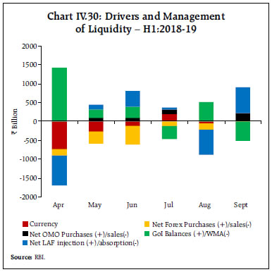 During Q1:2018-19, liquidity conditions remained generally in surplus, reflecting the drawdown of government balances due to transfer of GST proceeds to states in April and higher spending by the central government in June 2018. The unwinding of large government cash balances – amounting to ₹1.4 trillion in April – more than offset the drain on liquidity caused by two other autonomous factors – currency expansion by ₹743 billion and forex sales of ₹140 billion – during the month. Although government balances continued to unwind in May, the scale of forex sales picked up in May as well as June, and currency expansion continued to be higher than expected, resulting in a liquidity deficit in the system (Chart IV.30). Accordingly, the RBI injected liquidity through variable rate repo of various tenors, in addition to the regular 14-day repos, to tide over the liquidity tightness in the second half of June. Based on an assessment of the prevailing liquidity conditions, including the drainage of durable liquidity due to forex operations, two OMOs of ₹100 billion each were conducted by the RBI in May and June 2018. Overall, the surplus absorbed under the LAF moderated progressively during the quarter from an average daily net position of ₹496 billion in April to ₹142 billion in May and further to ₹140 billion in June. During Q2:2018-19, liquidity conditions gyrated. In July 2018, liquidity was generally in deficit due to moderation in government spending (especially in the second half of July) and the liquidity impact of the RBI’s forex sales, necessitating average daily net injection of ₹107 billion under the LAF (Chart IV.31). Besides, durable liquidity was also injected through OMO purchases amounting to ₹100 billion in July. The system again moved back into an absorption mode in August (up to August 19) due to increased spending and recourse to ways and means advances (WMA) by the government. Although systemic liquidity turned into deficit, necessitating liquidity injection between August 20 and 30, the RBI absorbed ₹30 billion on an average daily net basis during the month. The system moved back into surplus from August 31 - September 10 as government spending increased, thereafter, it turned into deficit. As a result, the RBI injected ₹406 billion on an average daily net basis during September. While durable liquidity needs were met through two OMO purchases amounting to ₹200 billion in the second half of September, day to day systemic liquidity surplus was managed by the RBI through variable rate reverse repos auctions and occasional liquidity deficits were met through regular 14-day variable rate term repos along with variable rate repos of other tenors. 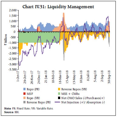 The key driver of liquidity during H1:2018-19 was the movement in government cash balances maintained with the RBI (Chart IV.32). Overall, the system liquidity remained in neutral mode for most part of H1, oscillating between surplus in the first quarter and largely deficit in the second quarter. As a part of the RBI’s continuous efforts to improve monetary policy transmission at the short-end of the money market, scheduled primary (urban) co-operative banks were provided access to the marginal standing facility (MSF), while scheduled state co-operative banks were provided access to both the LAF and the MSF on complying with the prescribed eligibility criteria. IV.4 Conclusion Domestic financial markets continue to remain vulnerable to evolving global developments, and especially, volatile capital flows. Unpredictability about the direction of capital flows has rendered market sentiment risk averse and uncertain. By contrast, the equity market has surged on the back of domestic institutional investors, even as there has been some correction in the recent period. Valuations, measured by conventional metric, are stretched, albeit driven by optimism on forward earnings. Elsewhere, credit growth has continued to improve. Going forward, liquidity conditions would be managed consistent with the stated policy objective of aligning the WACR with the policy repo rate and ensuring durable liquidity demands of the economy are met. Ensuring better monetary transmission continues to remain a priority for the RBI.
V. External Environment Global growth maintained pace, but asynchronously across regions. World trade growth has slowed down in recent months due to ongoing trade tensions clouding the overall outlook. Inflation pressures are building up in advanced economies (AEs) and emerging market economies (EMEs) on rising energy prices. Financial markets, particularly in EMEs, remained volatile given the ongoing normalisation of US monetary policy, crude price volatility and geopolitical tensions. Since the Monetary Policy Report (MPR) of April 2018, uncertainties have clouded the near term outlook for the global economy on several fronts. First, world trade is showing signs of slowdown with the intensification of trade wars. Second, crude prices are experiencing high volatility at elevated levels and risks of supply disruptions have been slanted to the upside by geopolitical tensions. Third, inflation pressures are building up in some AEs as well as in many EMEs, mainly on elevated energy prices. Consequently, even as global growth has maintained pace, it has diverged amongst regions/ economies – strong activity in North America and in several parts of Asia and Africa, but a weaker profile in Europe, China, Latin America and sub-Saharan Africa. Global financial markets have been unsettled by bouts of high turbulence and volatility, and swings in investor sentiment have become more pronounced in the recent period. A brewing cocktail of the ongoing monetary policy normalisation in the US, escalating trade conflicts and geopolitical tensions, persisting fears of crude price volatility and crisis conditions in some EMEs are intermittently triggering waves of risk aversion with respect to EMEs as an asset class and flight to safety. Equity markets have reflected these swings, scaling new highs in the US but with sharp selloffs in EMEs. Bond yields spiked in major AEs in April, but softened subsequently on safe haven demand, while they remained elevated in EMEs, impacted by global spillovers, including technical contagion. The US dollar’s persistent appreciation right up to mid- August has translated into currency depreciations in other AEs and EMEs. V.1 Global Economic Conditions Turning to macroeconomic conditions in major economies, annualised real GDP growth of the US surged above 4.0 per cent in Q2:2018 – the strongest in over three years – fuelled by tax cuts, robust consumer spending and steadily improving labour market conditions (Table V.1). Industrial output also strengthened, although the outlook is scoured by rising trade tensions. | Table V.1: Real GDP Growth (q-o-q, annualised) | | (Per cent) | | Country | Q2: 2017 | Q3: 2017 | Q4: 2017 | Q1: 2018 | Q2: 2018 | 2018 (P) | 2019 (P) | | Advanced Economies | | | | | | | | | Canada | 4.6 | 1.6 | 1.7 | 1.4 | 2.9 | 2.1 | 2.0 | | Euro area | 2.8 | 2.8 | 2.8 | 1.6 | 1.6 | 2.2 | 1.9 | | Japan | 2.0 | 2.3 | 0.9 | -0.9 | 3.0 | 1.0 | 0.9 | | South Korea | 2.4 | 5.6 | -0.8 | 4.0 | 2.4 | 3.0 | 2.9 | | UK | 1.2 | 1.6 | 1.6 | 0.4 | 1.6 | 1.4 | 1.5 | | US | 3.0 | 2.8 | 2.3 | 2.2 | 4.2 | 2.9 | 2.7 | | Emerging Market Economies | | | | | | | | | Brazil | 1.6 | 2.4 | 0.0 | 0.4 | 0.8 | 1.8 | 2.5 | | China | 7.6 | 7.2 | 6.4 | 5.6 | 7.2 | 6.6 | 6.4 | | Malaysia | 5.2 | 6.8 | 4.0 | 5.6 | 1.2 | 5.3 | 5.0 | | Mexico | 2.2 | -0.4 | 3.3 | 3.9 | -0.6 | 2.3 | 2.7 | | Russia* | 2.5 | 2.2 | 0.9 | 1.3 | 1.9 | 1.7 | 1.5 | | South Africa | 2.9 | 2.3 | 3.1 | -2.6 | -0.7 | 1.5 | 1.7 | | Thailand | 5.3 | 4.0 | 1.8 | 8.5 | 4.1 | 3.9 | 3.8 | | Memo: | 2017 (E) | 2018 (P) | 2019 (P) | | World output | 3.7 | 3.9 | 3.9 | | World trade volume | 5.1 | 4.8 | 4.5 | E: Estimate P: Projection *: y-o-y growth
Sources: Bloomberg; and International Monetary Fund. | The Euro area slowed down, with weak GDP growth in Q1:2018 extending into Q2. The manufacturing purchasing managers’ index (PMI) has declined during Q3:2018. A similar pattern was observed in other sentiment indicators like consumer confidence and business sentiment. Capacity utilisation declined in Q3:2018, while the unemployment rate has inched lower during Q3 so far, amidst persisting regional disparities. Political tensions and Brexit concerns, along with the ongoing trade conflicts, pose significant risks to the overall growth outlook. The Japanese economy expanded at a strong pace in Q2:2018 after contracting in the previous quarter, boosted by a rebound in household consumption and a rise in business spending. Capital expenditure also rose for the seventh quarter in a row. However, weak export orders and subdued business confidence indicate concerns surrounding trade protectionism. Economic activity has weakened in several EMEs. Financial deleveraging has weighed on GDP growth in China in Q2:2018 amidst rising trade tensions, which resulted in a current account deficit during H1:2018, a first in two decades. Weak infrastructure spending and falling retail sales are accentuating the slowdown. The combination of these factors poses major risks to the outlook. Among the other BRICS economies, headwinds from political uncertainties in May were reversed in Brazil in June, but economic activity remained subdued in Q2:2018, reflecting the lingering effects of the recession. In Russia, incoming data suggest that growth momentum was sustained in Q2:2018, supported by strong export growth and retail sales, with private consumption and improving labour market conditions likely to be growth drivers alongside firm crude prices. South Africa slipped into recession in Q2:2018 on account of the negative contribution from agriculture (due to a very large base effect) and adverse effects of political uncertainties. In Asia, where growth impulses have remained reasonably resilient to the global turmoil, the Indonesian economy picked up in Q2:2018, driven by private consumption and imports. In Thailand, growth moderated in Q2, pulled down by weaker government consumption although private consumption and strong farm incomes provided an offset. Growth eased in Q2 in Malaysia, dragged down by moderation in exports and strengthening import demand. Turkey is facing major downside risks from exchange rate pressures, geopolitical tensions, a widening current account deficit, soaring inflation, weakening public institutions and sovereign credit rating cuts moving it deeper into “junk” territory in August. This has heightened rollover risk with regard to US dollar denominated liabilities, especially of its corporate sector. The turbulent external sector outlook for Turkey since early August has had perverse spillovers to other EMEs due to a generalised build-up of risk aversion among investors. The global composite PMI indicates growth slowing down in Q3:2018 across manufacturing and service sectors (Chart V.1a). Among the major OECD economies, growth is expected to strengthen in the US and Japan, while it is expected to weaken in the UK, the Euro area (including Germany, France and Italy) and Canada. Among major EMEs, the composite leading indicators (CLIs) point to growth strengthening in China, remaining stable in Russia, but weakening in Brazil and South Africa (Chart V.1b). 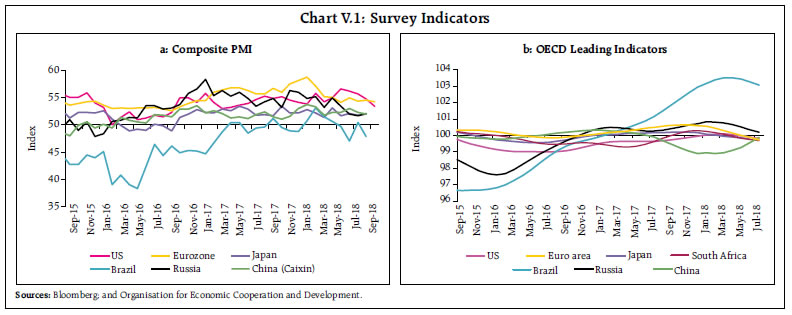 Global trade growth, in real terms, slowed down in 2018 (up to June), although the increase in commodity prices compensated for volume deceleration (Chart V.2a). For AEs, the loss of momentum has been somewhat higher than EMEs. Forward looking indicators suggest that world trade is likely to slow down further in the remaining part of 2018. The World Trade Outlook Indicator (WTOI)1– currently above trend – has eased in the last three quarters, dragged down by slowing export orders, international air freight and container port throughput. Movement in other indicators such as the Baltic Dry Index also point to a moderation in global trade (Chart V.2b). 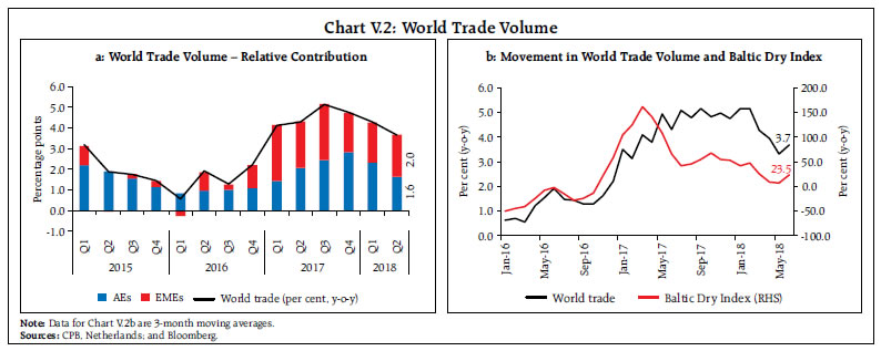 Trade wars weigh heavily on the outlook for global trade. Simulation analysis by the IMF2 suggests that global GDP could be lower by about 0.4 per cent in the first year and by about 0.5 per cent in the second year relative to the baseline. Tariffs on their own have a smaller effect on global GDP, with a maximum loss of about 0.1 per cent relative to the baseline. V.2 Commodity Prices and Inflation Global commodity price movements have been driven by commodity-specific demand-supply imbalances, strengthening of the US dollar and ongoing trade tensions. The Bloomberg commodity index declined by 2.6 per cent during April-September 2018. The food price index of the Food and Agriculture Organisation (FAO) fell by 3.2 per cent between April and August 2018 on account of a decline in the prices of most food items. International sugar prices, in particular, appear to be set for accentuated contraction due to increased supply from major suppliers on their currency depreciations (Chart V.3a). Crude oil prices surged by 20.0 per cent during April- September 2018. Brent prices rose incessantly between end-June and July on geo-political tensions relating to expected US sanctions on Iran and supply disruptions in Venezuela, Libya and Canada. Prices were also supported by robust demand (Chart V.3b). Base metal prices, measured by the Bloomberg base metal spot index, have fallen by 8.3 per cent between April and September 2018, pulled down by bearish sentiment as trade tensions escalated and global risk aversion ensued on Turkish turmoil in August. Copper prices, which surged in early June, have dropped substantially on a strong US dollar, trade tensions and expectations of weaker demand triggered by the selloffs in EMEs. Gold and silver prices have moderated on a resurgent US dollar (Chart V.4). 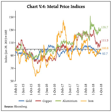 Inflation pressures are building up in most AEs and EMEs. Among AEs, CPI inflation in the US has remained steady at above 2.0 per cent since November 2017, supported by the tightening labour market and rising energy prices. The personal consumption expenditure (PCE), the Fed’s preferred measure of inflation, touched 2.0 per cent in May 2018 and has remained steady since then. Inflation in the Euro area has risen consistently to touch its highest level in 5½ years in July at 2.1 per cent. In Japan, inflation softened during Q2:2018 as rising energy prices were tempered by weak food prices, though an uptick was witnessed in Q3 on rising transport costs (Chart V.5a). Inflationary pressures in EMEs are also rising (Chart V.5b). In Turkey, inflation surged to 24.5 per cent in September, indicating the impact of the sharp currency depreciation. Inflation in Russia touched its highest level in one year in August on rising food prices. In Brazil, inflation has risen during H2:2018 so far due to disruptions in supplies caused by nation-wide strikes in May and hardening energy prices. China’s consumer price inflation rose to 2.3 per cent in August on higher food prices. In Indonesia, inflation remained below the central bank’s target of 3.5 per cent. V.3 Monetary Policy Stance Monetary policy is increasingly becoming less accommodative in most AEs and EMEs. The US Fed raised its policy rate thrice in 2018 and investors expect the rate to be raised one more time during this year and three times in 2019 (Chart V.6a). The European Central Bank (ECB) is normalising its monetary policy at a much slower pace; it will end its large scale asset purchase (LSAP) in a staggered manner by the end of 2018. The Bank of Japan (BoJ) has continued with its ultra-accommodative stance as inflation has remained well below the target. It tweaked its monetary policy operating procedures in July, providing more flexibility to the movement of yields, though the target for the long-term bond yield remains unchanged at zero. Monetary policy stances in EMEs are getting increasingly synchronised, with many central banks either increasing policy rates or keeping them unchanged. Among BRICS countries, Brazil and South Africa kept their policy rates unchanged. Russia raised its policy rate in September 2018, after a hiatus of almost four years, in response to inflationary risks. In Asia, Indonesia raised its policy rate five times since May 2018 to contain the currency’s slide. The People’s Bank of China has left its benchmark one-year lending and deposits rates unchanged since October 2015. However, it raised short-term interest rates in Q1:2018 and eased reserve requirements to free up liquidity in the system in June. Among other EMEs, Turkey has aggressively raised its policy rate by more than 1500 bps this year, cut reserve requirement by 250 basis points across all maturity brackets and lowered reserve requirement ratios for non-core FX liabilities by 400 basis points for up to three-year maturities in August. The central banks of Mexico and the Philippines raised their policy rates during the last two quarters on a worsening inflation outlook (Chart V.6b). 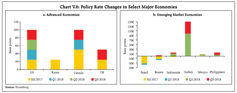 V.4 Global Financial Markets Volatility in global financial markets in H1:2018-19 has hit EMEs as an asset class, leading to capital outflows and currency depreciations. Global equity prices have been under presure on waning risk appetite, as geo-political developments across geographies and tightening liquidity conditions have triggered bearish sentiment and rebalancing of portfolios. Among AEs, equity prices have remained under pressure in the Euro area on slowing economic growth, trade tensions and concerns over the impact of the crisis in Turkey. Equity markets in the US have gained, largely driven by the technology sector. Equity indices have been further buoyed by the North American Free Trade Agreement (NAFTA) deal in September, despite the ongoing trade tensions. The relatively stronger performance of the US equity market vis-a-vis other AEs and EMEs reflected a flight to safety. In Japan, equity markets have risen encouraged by a weak currency, though subdued business confidence has capped gains. Equity markets in EMEs have declined on a general risk-off sentiment (Chart V.7). 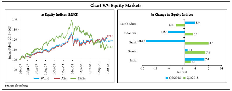 Global bond markets were visited by bouts of volatility due to a combination of factors – accelerating US growth and a weakening of economic activity in other AEs; trade tensions; geopolitical events; and expectations around an expansionary fiscal policy in the US. Sovereign bond yields have risen in most AEs and EMEs. 10-year bond yields are rising in the US on strong macroeconomic data, despite the ongoing trade tensions. The global financial crisis (GFC) has revealed that asset prices do not follow a normal distribution, which understates the dynamic nature of volatility. They show fatter tails, implying the occurrence of extreme events, often correlated across various assets. Such events have occurred more often in the US 10-year government securities since 2008 than in other asset classes, viz., stocks or commodities. The bond market in the US alone witnessed extreme outcomes several times in 2018. (Chart V.8). 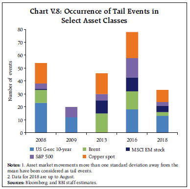 In the Euro area, the benchmark 10-year German bond yield moderated on worries over weak economic growth and budget concerns in Italy. In Japan, bond yields, which remained largely range bound during the year, have surged since end-July as the BoJ kept its long-term bond yield target unchanged at around zero per cent (Chart V.9a). Bond yields in EMEs reflected inter alia country-specific factors, though they have risen recently in most countries on expectations of shrinking global liquidity and tighter domestic monetary policy stances. 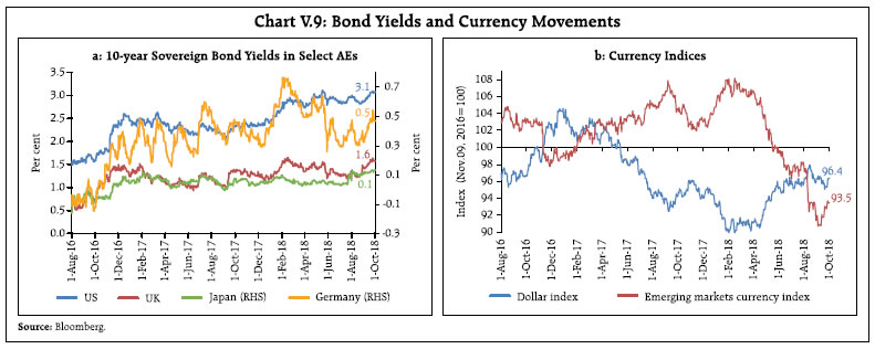 Currency markets have been driven largely by monetary policy stances in the systemically important AEs – particularly in the US, geo-political developments and country-specific factors. The US dollar appreciated between April and September on policy rate hikes thrice during the year, signalling the US Fed’s view that economic activity is growing at a robust clip. The euro lost ground to the US dollar on growth differentials and political tensions in some member states, with the recent Turkish turmoil and significant exposures to Turkey of European banks, exerting downward pressure on the euro. The Japanese yen depreciated driven by widening growth differentials with the US and accommodative monetary policy. Most EM currencies depreciated on capital outflows driven by global spillovers that also impacted bond markets (Chart V.9b). Between April and September 2018, the MSCI Emerging Market Currency Index declined by 7.0 per cent. Contagion from the collapse of the Turkish lira and the Argentine peso led to large depreciations across EM currencies in the second half of August 2018 as correlations with the Turkish lira and Argentine peso increased (Chart V.10). Many bystander central banks among EMEs undertook large scale forex interventions and/or monetary policy measures to contain volatility and calm currency markets. Against the backdrop of episodes of spillover to the EMEs, a comparison of current macroeconomic conditions vis-à-vis those characterising the taper tantrum of 2013 across five EMEs suggests that although economic fundamentals have generally improved, some weak spots still remain (Chart V.11). A noteworthy pattern that has emerged in the period following the GFC is that commodity prices have a significant bearing on movements in financial markets with strong inter-linkages across asset classes (Box V.1). This pattern implies important risk in the form of correlated volatility across financial markets, especially for EMEs, from the surging oil prices. Box V.1: Global Commodity Prices and Financial Markets in EMEs The sharp increase in commodity prices, especially of crude oil and base metals since the early 2000s, has led to financialisation of commodities through the rapid development of futures and other derivatives markets. Investors in these markets include banks, institutional investors, insurance companies, pension funds and individuals trying to optimise the risk-return profiles of their portfolios through index trading in derivatives. While doing so, they exploit arbitrage opportunities in commodity derivatives markets. While investment in commodity indices has increased significantly since the early 2000s, the impact of financialisation and risk spillovers has become clearer only after the GFC (European Central Bank, 2011; de Boyrie and Pavlova, 2016). Against this backdrop, the dynamic relationship between global energy market and other asset markets was examined in a vector autoregression (VAR) framework using monthly data from January 2001 to July 2018. In order to explore the role of financialisation, the VAR analysis is undertaken for two sub-samples, i.e., January 2001 to July 2008 (pre-GFC period) and August 2009 to July 2018 (post- GFC period). The World Bank energy (WBE) and World Bank non-energy (WBNE) indices were used to represent global commodity prices. The MSCI Emerging Market Equity Index3 (EMEQ) represents the performance of large- and mid-cap securities in 24 emerging markets and the MSCI Emerging Market Currency Index (EMCU) measures the total return of 25 emerging market currencies relative to the US dollar. These two indices were taken as proxies for the equity and currency markets, respectively. The J. P. Morgan Emerging Market Bond Index4 (EMBI) was taken as proxy for the bond market. As energy prices are more volatile than non-energy prices, a variable representing energy market financialisation, i.e., open active oil contracts (OILAC) was also included in the VAR model. Market volatility and policy-related uncertainty were proxied by the implied volatility of the S&P 500 index options (VIX) and the Economic Policy Uncertainty5 (EPU) index, respectively, as exogenous (pre-determined) variables. As all the endogenous variables were found to be non-stationary of order one, cointegrating relationship between them was examined through a vector error correction model (VECM) and impulse responses were formulated using the reduced form VAR model as given below: yt = A + BYt-p +DXt + ξt , where p is the order of the VAR model; and Yt is the vector of endogenous variables, viz., WBE, WBNE, EMEQ, EMCU, EMBI, OILAC; and Xt is the vector of exogenous variables, viz., VIX and EPU. The restricted cointegration rank tests (trace and maximum eigenvalue) confirm the presence of a single long-run cointegrating relationship among the variables with a lag of two, based on Akaike Information Criteria. The presence of a cointegrating relationship indicates that there exists a long-term relationship between the commodity price movements and other financial asset classes. As a robustness check, the VECM model confirms that residuals are not serially correlated. The reaction of a particular financial market segment to the initial commodity price shocks is examined through impulse response functions. Based on Cholesky decomposition, the impulse response analysis reveals that an energy price shock impacts the sovereign bond, currency and equity markets (Chart V.1.1). Bond yields rise due to expectation of tightening of monetary policy following the adverse impact of energy prices on inflation and the impact is found to be somewhat higher in the post-GFC period. Similarly, EME currencies depreciate and the impact is seen to be stronger during the post-GFC period, though the extent of depreciation varies depending on the quantum of imports of energy requirements. Equity markets are found to be affected adversely in the pre-GFC period as higher commodity prices may lower profit margins of corporates due to increase in input costs and also due to higher interest rates as central banks raise rates to contain inflation. In the post-GFC period, however, equity prices increase in the first few months after a shock to energy prices. One reason for this positive co-movement, as argued by Bernanke (2016), could be that both energy and equity prices are “reacting to a common factor, namely, a softening of global aggregate demand, which hurts both corporate profits and demand for oil”. Thus, the empirical analysis shows that energy price shocks have impacted the currency and bond markets in EMEs more in the post GFC period vis-à-vis pre-GFC period, underlining the greater role of financialisation of commodity markets. References: Bernanke, B. (2016), “The Relationship between Stocks and Oil Prices”, Brookings. Available at: https://www.brookings.edu/blog/ben-bernanke/2016/02/19/the-relationship-between-stocks-and-oil-prices/ de Boyrie, M. E., and, I. Pavlova (2016), “Linkages between Equity and Commodity Markets: Are Emerging Markets Different?”, Available at: https://acfr.aut.ac.nz/data/assets/pdf_file/0006/56445/42984-M-deBoyrie-Linkages-between-Equity-and-Commodity-Markets.pdf European Central Bank (2011), Monthly Bulletin, October. |
V.5 Conclusion In sum, global economic activity has so far remained resilient to ongoing trade conflicts, geo-political tensions and tightening financial conditions. However, financial market volatility has increased as investors continuously reassess the impact of unfolding events. More ominously, global trade growth has begun to slow down. The inflation outlook has deteriorated in many AEs and EMEs. These developments taken together will pose a major challenge to global growth prospects in the coming quarters and years.
ABBREVIATIONS | ADF | Augmented Dickey-Fuller | | AEs | Advanced Economies | | AIFIs | All India Financial Institutions | | AL | Agricultural Labourers | | ASEAN | Association of Southeast Asian Nations | | ARCH | Autoregressive Conditional Heteroscedasticity | | ARDL | Autoregressive Distributed Lag | | A2+FL | Actual paid out costs plus imputed value of family labor used in production | | BE | Budget Estimates | | BEI | Business Expectations Index | | BIS | Bank for International Settlements | | BoJ | Bank of Japan | | bps | Basis Points | | BRICS | Brazil, Russia, India, China and South Africa | | CASA | Current Account and Saving Account | | CBLO | Collateralised Borrowing and Lending Obligation | | CCIL | Clearing Corporation of India Ltd. | | CD | Certificate of Deposit | | CDS | Credit Default Swap | | CGST | Central Goods and Services Tax | | CI | Confidence Interval | | CII | Confederation of Indian Industry | | CLI | Composite Leading Indicator | | CMB | Cash Management Bill | | CMIE | Centre for Monitoring Indian Economy | | CP | Commercial Paper | | CPC | Central Pay Commission | | CPI | Consumer Price Index | | CPI-AL | Consumer Price Index for Agricultural Labourers | | CPI-IW | Consumer Price Index for Industrial Workers | | CPI-RL | Consumer Price Index for Rural Labourers | | CSO | Central Statistics Office | | CU | Capacity Utilisation | | CU (SA) | Capacity Utilisation (Seasonally Adjusted) | | DGCI&S | Directorate General of Commercial Intelligence and Statistics | | DISCOMs | Distribution Companies | | DXY | US Dollar Index | | ECB | European Central Bank/External Commercial Borrowings | | EMBI | Emerging Market Bond Index | | EMDEs | Emerging Market and Developing Economies | | EMEs | Emerging Market Economies | | EMEQ | Emerging Market Equity Index | | EMCU | Emerging Market Currency Index | | EPU | Economic Policy Uncertainty | | EU | European Union | | EWMA | Exponential Weighted Moving Average | | FAE | First Advance Estimate | | FALLCR | Facility to Avail Liquidity for Liquidity Coverage Ratio | | FAO | Food and Agriculture Organisation | | FBIL | Financial Benchmarks India Pvt. Ltd | | FCCB | Foreign Currency Convertible Bond | | FCI | Food Corporation of India | | FDI | Foreign Direct Investment | | FICCI | Federation of Indian Chambers of Commerce and Industry | | FMCG | Fast Moving Consumer Goods | | FIMMDA | Fixed Income Money Markets and Derivatives Association | | FPAS | Forecasting and Policy Analysis System | | FPI | Foreign Portfolio Investment/Investor | | FRBM | Fiscal Responsibility and Budget Management | | FX | Foreign Exchange | | FY | Financial Year | | GARCH | Generalised Autoregressive Conditional Heteroscedasticity | | GCF | Gross Capital Formation | | GDP | Gross Domestic Product | | GFC | Global Financial Crisis | | GFCE | Government Final Consumption Expenditure | | GFCF | Gross Fixed Capital Formation | | GFD | Gross Fiscal Deficit | | GIC | General Insurance Corporation | | GIC HFL | GIC Housing Finance Limited | | GNDI | Gross National Disposable Income | | G-Secs | Government Securities | | GST | Goods and Services Tax | | GSTN | Goods and Services Tax Network | | GVA | Gross Value Added | | GSDP | Gross State Domestic Product | | H1 | First Half of the Year | | H2 | Second Half of the Year | | HDFC | Housing Development Finance Corporation | | HFC | Housing Finance Company | | HNI | High Net Worth Individual | | HRA | House Rent Allowance | | IBC | Insolvency and Bankruptcy Code | | ICR | Interest Coverage Ratio | | IGST | Integrated Goods and Services Tax | | IIP | Index of Industrial Production | | IL&FS | Infrastructure Leasing and Financial Services Limited | | IMD | India Meteorological Department | | IMF | International Monetary Fund | | INR | Indian Rupee | | IO | Input-Output | | IOCL | Indian Oil Corporation Limited | | IOS | Industrial Outlook Survey | | IT | Information Technology | | IPO | Initial Public Offering | | KLEMS | Capital (K), Labour (L), Energy (E), Materials (M) and Services (S) | | LAF | Liquidity Adjustment Facility | | LCR | Liquidity Coverage Ratio | | LIBOR | London Interbank Offered Rate | | LIC | Life Insurance Corporation of India | | LIC HFL | LIC Housing Finance Limited | | LPA | Long Period Average | | LPG | Liquefied Petroleum Gas | | LSAP | Large Scale Asset Purchase | | MCLR | Marginal Cost of Funds Based Lending Rate | | MEP | Minimum Export Price | | MFs | Mutual Funds | | m-o-m | Month-on-Month | | MPC | Monetary Policy Committee | | MPR | Monetary Policy Report | | MSCI | Morgan Stanley Capital International | | MSF | Marginal Standing Facility | | MSP | Minimum Support Price | | MSS | Market Stabilisation Scheme | | MTM | Mark-to-Market | | MVKF | Multivariate Kalman Filter | | NAFTA | North American Free Trade Agreement | | NBFCs | Non-Banking Financial Companies | | NDSI | Non-Deposit Systemically Important | | NCAER | National Council of Applied Economic Research | | NCD | Non-Convertible Debentures | | NDTL | Net Demand and Time Liabilities | | NEER | Nominal Effective Exchange Rate | | NFC | Non-Food Credit | | NHB | National Housing Bank | | NPA | Non-Performing Asset | | NRI | Non-Resident Indian | | NSDL | National Securities Depository Limited | | NSE | National Stock Exchange | | NSSF | National Small Savings Fund | | OD | Over Draft | | OECD | Organisation for Economic Co-operation and Development | | OG | Output Gap | | OILAC | Open Active Oil Contracts | | OMCs | Oil Marketing Companies | | OMOs | Open Market Operations | | OPEC | Organisation of the Petroleum Exporting Countries | | PADO | Public Administration, Defence and Other Services | | PCA | Prompt Corrective Action | | PCE | Personal Consumption Expenditure | | PD | Primary Dealer | | PFCE | Private Final Consumption Expenditure | | PM AASHA | Pradhan Mantri Annadata Aay Sanrakshan Abhiyan | | PMAY | Pradhan Mantri Awas Yojana | | PMI | Purchasing Managers’ Index | | PRN | Production-weighted Rainfall Index | | PSU | Public Sector Undertaking | | Q1 | First Quarter | | Q2 | Second Quarter | | Q3 | Third Quarter | | Q4 | Fourth Quarter | | QE | Quantitative Easing | | q-o-q | Quarter-on-Quarter | | QPM | Quarterly Projection Model | | RBI | Reserve Bank of India | | RE | Revenue Expenditure/Revised Estimate | | REER | Real Effective Exchange Rate | | RERA | Real Estate (Regulation and Development) Act | | RHS | Right Hand Side | | RL | Rural Labourers | | RRBs | Regional Rural Banks | | SAAR | Seasonally Adjusted Annualised Rate | | SCBs | Scheduled Commercial Banks | | SDF | Standing Deposit Facility | | SDLs | State Development Loans | | SEBI | Securities and Exchange Board of India | | SGST | State Goods and Services Tax | | SLR | Statutory Liquidity Ratio | | SME | Small and Medium Enterprise | | SPD | Standalone Primary Dealer | | S&P | Standard & Poor’s | | T-Bill | Treasury Bill | | TFP | Total Factor Productivity | | UCM | Unobserved Components Model | | UK | United Kingdom | | US | United States | | US$ | US Dollar | | VAR | Vector Autoregression | | VECM | Vector Error Correction Model | | VIX | S&P 500 Volatility Index | | WACR | Weighted Average Call Money Rate | | WADTDR | Weighted Average Domestic Term Deposit Rate | | WALR | Weighted Average Lending Rate | | WBE | World Bank Energy | | WBNE | World Bank Non-Energy | | WMA | Ways and Means Advances | | WPI | Wholesale Price Index | | WTI | West Texas Intermediate | | WTO | World Trade Organisation | | WTOI | World Trade Outlook Indicator | | y-o-y | Year-on-Year | |