Press Release

RBI Working Paper Series No. 05
India’s Investment Cycle: An Empirical Investigation

^@Janak Raj
Satyananda Sahoo
and
Shiv Shankar

Abstract

¹This study estimates the duration of the investment cycle and examines the determinants of investment activity in India. Using the National Bureau of Economic Research (NBER) dating procedure, the study finds that the real investment rate in India followed a three-year cycle during the period from 1950-51 to 2017-18, with broadly nine episodes of contraction/upturn of two years and above. Investment activity in India declined sharply from 2011-12 to 2015-16. Decomposition of investment activity suggests that while the trend component has consistently moderated from 2011-12 onwards, the cycle component has turned from 2016-17. The current upturn in the investment cycle is estimated to last up to 2022-23 when the investment rate could rise to 33.0 per cent from the current rate of 31.4 per cent. Economic activity, real interest rate and bank credit were the major determinants of investment activity in India. The gross fiscal deficit crowds out investment activity.

JEL Classification Codes: E22, E32

Keywords: Investment rate, investment cycle, business cycle, expansion, contraction, determinants of investment.

Introduction

The Indian economy is domestic demand driven with consumption and investment playing key roles in growth dynamics. Investment activity, in particular, is significant as it not only plays an important role in shaping the current growth rate of the economy, but also in boosting the country’s medium-term growth prospects. In the post-Independence period, the real investment rate² in India generally trended upwards to peak at 36.7 per cent in 2007-08, before declining to 30.3 per cent by 2015-16 due to a variety of factors such as the adverse impact of the global financial crisis, the twin balance sheet problem – high leverage by the corporate sector and high non-performing assets (NPAs) of the banking sector, and subdued domestic capital market conditions. The slowdown in the investment rate was one of the major factors, which pulled down India’s growth rate from a high of 9.3 per cent in 2007-08 to a low of 6.7 per cent in 2017-18. Though the investment rate has picked up since 2016-17, there is uncertainty about the sustainability of the recent upturn in investment activity and its role in stepping up India’s growth rate – both in the near- and the medium-term.

Against this backdrop, this paper examines two issues. First, whether the current pick up in investment activity is sustainable. If so, how long is the current investment cycle expected to last? While a good amount of research has been conducted to study the growth or business cycles, there is hardly any study at the aggregate level on the investment cycle – either in advanced economies (AEs) or emerging market economies (EMEs), including India. The present study is an attempt to fill this critical gap in the Indian context. Second, what are the major determinants of investment activity in India?

The study uses the National Bureau of Economic Research (NBER) dating procedure for measuring the duration of the investment cycle in India and its sustainability. The study finds that the investment rate in India has followed, on an average, a three-year duration of cycle during the post-independence period. While the average duration of speed-up (trough to peak) was 1.6 years (seven quarters), the average duration of slowdown (peak to trough) was 1.4 years (five quarters). The decline in investment activity from 2011-12 to 2015-16 was led by a decline in both trend and cyclical factors. While the trend investment rate has continued to decline thereafter, there has been a cyclical upturn since 2016-17. The empirical estimates suggest that the current upturn in the investment cycle is likely to last up to 2022-23 when the investment rate is estimated to peak at 33.0 per cent. The study also finds that GDP growth, real interest rate and bank credit are the major determinants of investment activity in India. The gross fiscal deficit (GFD) crowds out private sector investment in India.

This paper is divided into five sections. Section II provides a brief survey of the available literature. The methodology used in the paper is explained in Section III. Empirical findings are analysed in Section IV. The concluding observations are set out in Section V.

II. Review of Literature

There are a number of studies on determining the chronology of business cycles. The study by Chitre (1982) was perhaps the first one to estimate growth cycles in the Indian context. Following the classical NBER procedure, Dua and Banerji (1999) estimated the business cycle and the growth rate cycle dates for the Indian economy. Mall (1999) used the growth cycle approach to filter the cyclical behaviour of industrial output of the Indian economy from 1950-51 to 1995-96. He found six sets of turning points in the manufacturing sector during the sample period. Patnaik and Sharma (2002) identified four episodes of contraction from 1950-51 to 1999-2000. They suggested that the use of the growth cycle approach was more suitable for extracting cycles in the post-liberalisation period. Using the monthly index of industrial production (IIP) series, Mohanty et al. (2003) identified 13 growth cycles of varying durations from 1970-71 to 2001-02. In their study, the average duration of cycles was 27 months, where the average duration of recession was 16 months, while the average duration of the expansion was 12 months. Using the growth cycle approach, Chitre (2001) identified eight peaks and eight troughs by constructing an index based on 94 monthly indicators for the period 1951-1982. Dua and Banerji (2012) constructed a composite leading index and reported seven business cycle recessions in the Indian economy for the period 1964-1996. They found that business cycle downturns in the pre-liberalisation period were associated either with drought or with oil price hike, while in the post-liberalisation period they were associated with dotcom bubble, swings in capital flows and the global financial crisis.

Ghate et al. (2013) examined the changing nature of Indian business from 1950 to 2010 by comparing the post-liberalisation phase with the pre-liberalisation phase. They found that the key macroeconomic variables were less volatile in the post-reform period as compared with the pre-reform period. More recently, Pandey et al. (2017) used the growth cycle approach to identify the chronology of business cycle turning points in the post-reform period. They identified three main episodes of recession from 1996 to 2014 and argued that characteristics of Indian business cycle turning points have changed over time. Furthermore, longer duration cycles were accompanied by greater variability in duration and amplitude of expansions/ recessions.

Some studies have examined the nature and causes of investment slowdown in the Indian context. A study by the Reserve Bank of India (RBI, 2013) finds that a 100 bps increase in the real interest rate leads to a decline of about 50 bps in the investment rate. Anand and Tulin (2014) found that while real interest rates accounted for only one quarter of the investment downturn, business confidence and economic policy uncertainty were the major factors in explaining the slowdown. Furthermore, despite softening of lending rates, sluggish credit offtake from the banking system – mainly due to subdued state of the economic activity, risk aversion in the banking sector due to high NPAs, capital adequacy requirements, highly leveraged corporate sector and uncertain global environment – had adversely impacted investment activity. The downturn in investment activity has also been led by a sharp decline in the growth of capital goods production. A recent study by Das and Tulin (2017) found that financial frictions have played an important role in investment slowdown in India. According to them, firms with higher financial leverage and lower earnings relative to their interest expenses invested less.

III. Methodology

There are two broad approaches, viz., the dating procedure and the production function approach for measuring business cycles. However, the dating procedure is preferred and widely used in view of the inherent problems associated with the measurement of technology shocks in a production function framework. Hence, we have used the dating procedure in this study.

NBER Dating Method

The measurement of an investment cycle is akin to the measurement of a business/economic cycle as investment activity like the business/economic cycle also works in two opposite directions, viz., a period of relative growth and expansion, followed by a period of decline and contraction and so on. The modern thinking on the business cycle could be traced back to Mitchell (1927) and Burns and Mitchell (1946). They defined the business cycle as: “…a cycle consists of expansions occurring at about the same time in many economic activities, followed by similarly general recessions, contractions and revivals which merge into the expansion phase of the next cycle”. The early NBER approach identified cycle, which occurs in two steps: (i) identifying cyclical peaks and troughs in the observed economic variables; and (ii) determining whether these changes were common enough through all the observed series. In this method, identification of a business cycle was based on absolute changes in the general level of production (Skare and Stjepanović, 2016).

A decline in key real economic variables in major industrial economies during the 1960s, however, led to an examination of accelerations or slowdowns in the growth rate rather than expansions or contractions in levels for identifying cycles (Mintz, 1974). In this approach, a growth cycle was defined as the ups and downs in the deviations of the actual growth rate of the economy from the long-run trend growth rate (Zarnowitz, 1992). In the growth cycle approach, expansion and contraction of a business cycle are of approximately the same duration. Boschan and Banerji (1990) argued that while growth cycles were not hard to identify in a historical time series, they were difficult to measure accurately on a real-time basis. This is because any measure of the most recent trend is necessarily an estimate and subject to revisions, and hence, it is difficult to precisely determine the growth cycle dates on a real time basis. They devised the growth rate cycle approach where cyclical upswings and downswings in the growth rate of economic activity are analysed.

As the NBER business cycle dating procedure is based on considerable amount of judgment, adequate precaution needs to be exercised to filter out false turning points from noisy data. The algorithm developed by Bry and Boschan (1971) and subsequently quantified by Harding and Pagan (2002) follows a set of simple rules for taking decision: (i) a peak is followed by a trough and a trough by a peak; (ii) each phase (peak to trough or trough to peak) must have a duration of at least six months or two quarters; (iii) a business cycle from peak to peak or trough to trough should have a duration of at least 15 months or five quarters in order to distinguish business cycles from seasonal cycles; and (iv) turning points are avoided at extreme points.

Since we observed a decline in real investment rate (in absolute terms) in India on many occasions during the post-1950 period, identification of cyclical peaks and troughs in levels was assessed to be more suitable than the growth rates. Therefore, we have followed the business cycle method of NBER as given below:

Extraction of Cycles: Univariate Methods

For the measurement of the duration of a cycle, it is very important to extract the cyclical component of a series. In practice, several alternative methods have been used to extract trend and cyclical components of observed time series. While the Hodrick and Prescott (1997) filter is a commonly used method, a major limitation of this method is that the estimated cyclical component is sensitive to the values of the smoothing parameter. There is another method based on the spectral analysis of the economic time series, viz., frequency or band-pass (BP) filter. The BP filters proposed by Baxter and King (1999) and Christiano and Fitzgerald (2003) eliminate very slow moving trend components and very high frequency components while retaining the intermediate business cycle fluctuations. As a result, BP filters retain the components that are associated with the periodicity of a typical business cycle. Moreover, these filters are time-invariant and symmetric with fixed weights, i.e., they do not change the relationship between time series at any frequency. A limitation of these filters, however, is that the end-points are lost due to lags and leads. To overcome this problem, Christiano-Fitzgerald (2003) suggested time-variant asymmetric filter with optimal finite-sample approximations for every observation in the sample. This method does not exclude end-points. This study uses all the four filters for extracting the cyclical and trend components (Annex I).

Multivariate Analysis

Past empirical studies suggest that investment activity is influenced by several domestic and global macroeconomic developments. Therefore, an attempt has also been made to assess the role of macroeconomic factors in determining investment activity through multivariate analysis.

In the case of capital-deficient developing countries, capital formation is the key driver of economic growth. The Economic Survey (Government of India, 2018) finds that one percentage point fall in investment rate dents growth by 0.4-0.7 percentage points. Investment rate is also highly correlated with the non-agriculture GDP growth rate, particularly in recent years (Chart 1).

The cyclical components of the real GDP growth rate co-move closely with the cycles extracted from the growth rate of real GFCF and the real investment rate (Chart 2).

Interest rate is one of the major factors in investment decisions. Starting with the standard neoclassical theory (Jorgenson, 1963), real interest rate, i.e., user cost of capital, plays an important role in capital formation. The negative relationship between real interest rate³ and investment rate in India is also evident after the 1990s when interest rates were deregulated (Chart 3).

Apart from the cost of capital, availability of financial resources/funds is another important factor that is expected to drive investment, especially because India has a bank-dominated financial system. Non-food credit growth of commercial banks is closely related with the investment rate (Chart 4).

The private sector is the biggest contributor to gross capital formation and it has played a crucial role in driving India’s investment activity. However, the fiscal deficit in India appears to have crowded out private investment as is evident from the negative relationship between the GFD and the investment rate (Chart 5).

Global growth is also observed to have an important bearing on India’s investment activity through exports. For instance, the GFC during the second half of the 2000s impacted the Indian economy through trade and finance channels. The global GDP growth turned negative in 2008 and 2009. Sluggish global economic activity dampened India’s export demand and led to a slowdown in investment activity (Chart 6).

The above relationships were formally tested using the following equation:

where,

I = Real investment rate (INVESTR)
g = Real GDP growth rate (GROWTH)
r = Real interest rate (RRATE, i.e., weighted average lending rate – expected inflation)
c = Non-food credit growth rate (NFC)
fd = Gross fiscal deficit as per cent of GDP (GFDR)
wg = Growth rate of world GDP (WGDP)

Real GDP growth rate represents demand conditions, i.e., a higher GDP growth means higher incomes, which then leads to higher investment activity. The real interest rate is a proxy for cost of borrowing which is expected to be inversely related with investment activity. Non-food credit is expected to have a positive sign. A higher level of the fiscal deficit could crowd out private investment as higher market borrowing by the Government to finance the deficit could impact resource raising by the private sector. The growth rate of world GDP is taken as a proxy for global demand, which is expected to be positively related to real investment.

IV. Empirical Findings

Investment Cycle Chronology

We have used annual real GFCF rate, i.e., real GFCF as percentage of real GDP as the measure of investment activity for the period 1950-51 to 2017-18 for our analysis⁴. As the real GFCF rate has declined in levels on many occasions during the post-1950 period, cyclical peaks and troughs are easy to identify in the realised levels than in the growth rates. Significantly, the growth rate of GFCF and the investment rate cycle, measured by the Christiano-Fitzgerald BP filter, are highly correlated (Chart 7).

While the trend and cyclical components, measured by the BP filters largely co-move, those measured by the HP filter slightly diverge from other filters possibly due to its sensitivity to the smoothing parameter λ, which has been taken as 100 as is normally the case for annual data. Based on all the filters, the trend component of the investment rate has moderated since 2011-12. However, the cyclical component has shown an upward movement from 2016-17 (Chart 8).

For the purpose of measuring the duration of the investment cycle, we use the cyclical factors extracted by the Christiano and Fitzgerald asymmetric BP filter as this method assigns variable weights and does not exclude end-points. Following the business cycle approach of the NBER, it is observed that the investment rate in India has, on an average, followed a cycle of three years duration in the post-independence period⁵ (Table 1).

While the average duration of expansion or speed-up (from trough to peak) was 1.6 years (seven quarters), the average duration of slowdown (from peak to trough) was 1.4 years (five quarters). From 1950-51 to 2017-18, there were broadly nine phases of contraction/expansion of two years and above (Chart 9). The largest decline in investment activity from 2011-12 to 2015-16 was led by a deceleration in both the trend and cyclical factors.

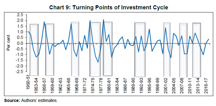In the post-liberalisation period, four downturns in the investment cycle were of a relatively larger magnitude (Chart 9). The first phase of severe downturn was in the first half of the 1990s, when the Indian economy was hit hard by the balance of payments crisis, leading to import compression and a deceleration in domestic economic activity. The next phase of downturn in the investment cycle occurred in the early 2000s due to an adverse impact of the bursting of the information technology bubble. The average real GDP growth from 2000-01 to 2002-03 decelerated to 4.5 per cent from 7.0 per cent in the second half of the 1990s. A sharp decline in the software exports due to the “Y2K” problem also dampened the investment cycle during this phase. The third phase of downturn during 2008-10 reflected knock on impact on the Indian economy through the trade, finance and confidence channels, resulting from the global financial crisis and seizure of the international capital market.

The last phase of downturn in the investment cycle occurred from 2011-12 to 2015-16, reflecting a combination of global and domestic factors. During this phase, world GDP growth fell from 4.3 per cent in 2011 to 3.2 per cent in 2016; average domestic inflation was around eight per cent; real interest rate measured by the difference between the weighted average lending rate (WALR) and expected inflation was high at around five per cent; the combined GFD of the Centre and states was on an average of 7.1 per cent; and the average current account deficit was 2.6 per cent. Bank credit growth collapsed as domestic commercial banks became risk averse due to large gross NPAs and the corporate sector focused on deleveraging rather than fresh investments.

The investment rate began to turn around from 2016-17. This is also reflected in several other high frequency indicators such as industrial production which has picked up since the H2:2017-18. Capital goods production, in particular, has increased sharply, reflecting strengthening of capital formation (Chart 10).

Bank credit growth (y-o-y) of scheduled commercial banks (SCBs), which decelerated from 21.3 per cent in March 2011 to 4.5 per cent in February 2017, has also shown a gradual pick-up from Q3:2017-18. The recent improvement in credit growth is also becoming increasingly broad-based. Credit flows to industry, which contracted during October 2016 to October 2017, has turned positive since November 2017 (Chart 11).

Resource mobilisation through initial public offerings (IPOs), which has been picking up since 2015-16, rose sharply in 2017-18 (Chart 12).

Capacity utilisation in the manufacturing sector, which plays a significant role in promoting fresh investment activity, has also picked up since H2:2017-18 and has reached the long-term average level in Q4:2017-18 (Chart 13).

The investment rate has picked up from 2016-17. During the last high growth phase from 2003-04 to 2007-08, the real investment rate remained in the upward trajectory continuously for five years. Forecasts based on various forms of univariate ARIMA models also suggest that the current investment cycle may last for five years up to 2022-23 when the real investment rate is estimated to increase further up to 33.0 per cent from the current level of 31.4 per cent in 2017-18.

Multivariate Analysis

Based on the availability of a common data set, the multivariate model as specified in equation 1 in Section III was estimated for the period from 1975-76 to 2017-18. The real interest rate (RRATE) was defined as the difference between nominal interest rate and expected inflation, i.e., one-period ahead inflation. We used three variants of the nominal interest rate, viz., weighted average lending rate (WALR), overnight call money rate (CALL) and 91-day Treasury Bills rate (TBILL91). Although all the three measures of real interest rates were found to be highly correlated, we used all of them for the purpose of our multivariate analysis (Annex II). World GDP growth (WGDP) represented global demand. The estimated model included two dummy variables, viz., DUM1 representing the phase of high capital flows (between 2002 and 2006) and DUM2 representing the global financial crisis between 2008 and 2010. Details of data definitions and sources are given in Annex III.

Before proceeding with the estimation procedure, the unit root properties of the series were examined. Barring real investment rate (INVESTR) and the GFD to GDP ratio (GFDR), all other variable were non-stationary at levels (Table 2). However, all the variables were stationary at the first differences.

As some of the variables were non-stationary, we adopted the autoregressive distributed lag (ARDL) model following Pesaran and Shin (1995, 1999), and Pesaran, et al. (1996) as standard ordinary least squares or Johansen-Juselius (1990, 1992) cointegration and vector error correction model (VECM) framework could lead to spurious/inconsistent estimates. The ARDL approach provides consistent estimates of the existence of relationships between variables, irrespective of whether the regressors are purely I(0), purely I(1), or a mixture of both (Annex IV). The estimated long-run coefficients obtained from ARDL models with three variants of real interest rate are given in Table 3.

In the estimated cointegrating equations, the long-run coefficients of all the explanatory variables are statistically significant and have expected signs. Furthermore, all the three specifications have valid error correction model as the short-run adjustment parameters are statistically significant and have expected negative signs (Annex V). The estimated models satisfy structural stability properties in terms of CUSUM and CUSUMSQ tests (Annex VI, Chart A2). The estimated models fit data very well as can be seen from the co-movement of actual and fitted values of the dependent variable (Annex VI, Chart A3). The in-sample forecast performance of the estimated model was found to be robust as the root mean square error and Theil inequality coefficient were found to be low.

As can be seen from Table 3, there are no discernible differences in the estimated parameters across the three models. The coefficient of real interest rate implies that a one percentage point increase in the real lending rate reduces the real investment rate in the range of 0.3 to 0.4 percentage points. Coefficients of real GDP growth ranged between 2.6 to 3.0 and they also had a higher lag order in the estimated model, implying that past economic performance plays a key role in investment decisions. Statistically significant and positive sign of the coefficient for non-food credit indicates that availability of funds has a significant bearing on investment activity. A negative coefficient for the GFD implies that the government borrowing crowds out private investment. A one percentage point increase in the GFD reduces investment demand by almost 0.5 percentage points.

V. Concluding Remarks

This paper was an attempt to examine in the Indian context: (i) the duration of the investment cycle; and (ii) major determinants of investment activity. Using the NBER dating procedure, the study finds that the duration of the investment cycle in India, on an average, was three years. The chronology of turning points reveals that while the average duration of speed-up (from trough to peak) was 1.6 years (seven quarters), the average duration of slowdown (from trough to peak) was 1.4 years (five quarters). From 1950-51 to 2017-18, there were broadly nine episodes of contraction/upturn phases of two years and above. Of these, four phases of downturn in the post-liberalisation period have been of severe magnitude, viz., (i) first half of the 1990s; (ii) early 2000s; (iii) 2007-08 to 2009-10; and (iv) 2011-12 to 2015-16.

The study finds that there has been a moderation in the trend component of the investment activity from 2011-12 onwards. However, the cyclical component has shown upward movement from 2016-17, suggesting that recent improvement in investment activity is due to cyclical factors. The upturn in the current investment cycle, which began in 2016-17, is estimated to last up to 2022-23 when the investment rate is estimated to increase up to 33.0 per cent from the current level of 31.4 per cent. However, the challenge is to reverse the declining trend component of investment activity. This will require policy efforts on multiple fronts such as further improving ease of doing business; expediting resolution of distressed assets; addressing the NPAs problem of the banking sector; and speeding up implementation of the stalled projects. These measures will help (i) ride the current phase of the investment cycle to its peak; and (ii) boost medium-term prospects of investment activity. The sharp acceleration in real GDP growth in Q1:2018-19, acceleration in bank credit growth and buoyant stock market augur well for sustaining investment activity going forward. However, uncertainties on the global front and financial market volatility need to be guarded against.

The study also finds that investment activity in India is affected by several macro-financial factors. These are real GDP growth, real interest rate, bank credit growth, global GDP growth and GFD. Domestic economic activity turned out to be the main determinant of investment activity in India. The real interest rate had a negative impact on investment activity. A one percentage point increase in the real lending rate reduces the real investment rate in the range of 0.29-0.40 percentage points. Non-food bank credit growth positively impacts investment activity. The GFD crowds out investment demand.

This study is a small, but an important step in unravelling some of the key aspects of investment activity in India. However, it may be useful to examine the investment cycle at the sectoral level and with high frequency quarterly data. The study could also be extended by adding some measure of economic policy uncertainty and indicators of business confidence in the multivariate analysis.

^@ Janak Raj, Satyananda Sahoo and Shiv Shankar are Principal Adviser, Director and Assistant Adviser, respectively, in the Monetary Policy Department, Reserve Bank of India, Mumbai.

¹ The authors are grateful to Dr. Viral V. Acharya and Dr. Michael Debabrata Patra and Shri Muneesh Kapur for their valuable comments/suggestions. We thank participants, in particular, the discussants Prof. Neeraj Hatekar and Shri A. K. Shukla, for their comments at a seminar at the Reserve Bank of India. The views expressed in the paper are those of the authors and not necessarily of the institution to which they belong.

² The real investment rate is defined as the ratio of real gross fixed capital formation (GFCF) to real gross domestic product (GDP).

³ Real interest rate = weighted average lending rate (t) – inflation rate (t+1).

⁴ Although quarterly data are available from 1996-97, they pertain to three different base years. Moreover, dating business cycle for a longer period historical series could provide better insights than the shorter one.

⁵ Preliminary analysis based on seasonally adjusted quarterly data for the period from Q1:1996-97 to Q4:2017-18, after converting them to a common base year, reveals that investment rate has a duration of 14 quarters, i.e., around 3.5 years.

⁶ This section heavily draws from Sahoo (2014).

References

Anand, R., &. Tulin, V. (2014). Disentangling India’s Investment Slowdown, IMF Working Paper, WP/14/47.

Baxter, M., & King, R. G. (1999). Measuring Business Cycles: Approximate Band-Pass Filters for Economic Time Series. Review of economics and statistics, 81(4), 575-593.

Boschan, C. & Banerji, A. (1990). A Reassessment of Composite Indexes. In P.A. Klein (ed.), Analyzing Modern Business Cycles, Armonk, New York: ME Sharpe.

Bry, G., & Boschan, C. (1971). Programmed Selection of Cyclical Turning Points. In Cyclical Analysis of Time Series: Selected Procedures and Computer Programs (pp. 7-63). National Bureau of Economic Research, Retrieved from: http://www.nber.org/chapters/c2145.

Burns, A. F., & Mitchell, W. C. (1946). Measuring Business Cycles, National Bureau of Economic Research. New York.

Chitre, V.S. (1982). Growth Cycles in the Indian Economy, Artha Vijnana, 24, 293-450.

Christiano, L. J., & Fitzgerald, T. J. (2003). The Band Pass Filter. International Economic Review, 44(2), 435-465.

Das, M. S., & Tulin, M. V. (2017). Financial Frictions, Underinvestment, and Investment Composition: Evidence from Indian Corporates, IMF Working Paper, WP/17/134.

Dua, P. & Banerji, A. (1999). An Index of Coincident Economic Indicators for the Indian Economy, Journal of Quantitative Economics, 15, 177-201.

Dua, P., & Banerji, A. (2012). Business and Growth Rate Cycles in India, Working papers 210, Centre for Development Economics, Delhi School of Economics.

Ghate, C., Pandey, R., & Patnaik, I. (2013). Has India emerged? Business Cycle Stylized Facts from a Transitioning Economy. Structural Change and Economic Dynamics, 24, 157-172.

Government of India (GoI) (2018), Economic Survey 2017-18.

Harding, D., & Pagan, A. (2002). Dissecting the Cycle: A Methodological Investigation. Journal of Monetary Economics, 49(2), 365-381.

Hodrick, R. J., & Prescott, E. C. (1997). Postwar US business cycles: An Empirical Investigation. Journal of Money, Credit, and Banking, 1-16.

Johansen, S., & Juselius, K. (1990). Maximum Likelihood Estimation and Inference on Cointegration—with applications to the demand for money. Oxford Bulletin of Economics and statistics, 52(2), 169-210.

Johansen, S., & Juselius, K. (1992). Testing Structural Hypothesis in a Multivariate Cointegration Analysis of PPP and the UIP for UK, Journal of Econometrics, 53, 211-44.

Jorgenson, D. W. (1963). Capital Theory and Investment Behavior. The American Economic Review, 53(2), 247-259.

Mall, O. P. (1999). Composite Index of Leading Indicators for Business Cycles in India. RBI Occasional Papers, 20(3), 373-414.

Mintz, I. (1974). Dating United States Growth Cycles. In Explorations in Economic Research, Volume 1, Number 1 (pp. 1-113). NBER.

Mohanty, J., Singh, B., & Jain, R. (2003). Business Cycles and Leading Indicators of Industrial Activity in India, MPRA Paper No. 12149, University Library of Munich, Germany.

Pandey, R., Patnaik, I., & Shah, A. (2017). Dating Business Cycles in India. Indian Growth and Development Review, 10(1), 32-61. https://doi.org/10.1108/IGDR-02-2017-0013

Patnaik, I., & Sharma, R. (2002). Business Cycles in the Indian Economy. MARGIN-NEW DELHI-, 35, 71-80.

Pesaran, M. H. (1997). The Role of Economic Theory in Modelling the Long Run. The Economic Journal, 107(440), 178-191.

Pesaran, M. H., & Shin, Y. (1995). Autoregressive Distributed Lag Modelling Approach to Cointegration Analysis, DAE Working Paper Series No. 9514, Department of Applied Economics, University of Cambridge.

Pesaran, M. H., & Shin, Y. (1999). Autoregressive Distributed Lag Modelling Approach to Cointegration Analysis. In Storm, S., (ed.), Econometrics and Economic Theory in the 20th. Century: The Ragnar Frisch Centennial Symposium. Cambridge University Press: Cambridge.

Pesaran, M. H., Shin, Y., & Smith, R. J. (1996). Testing the Existence of a Long-Run Relationship, DAE Working Paper Series No. 9622, Department of Applied Economics, University of Cambridge.

Pesaran, M. H., Shin, Y., & Smith, R. J. (2001). Bounds Testing Approaches to the Analysis of Level Relationships. Journal of Applied Econometrics, 16(3), 289-326.

Reserve Bank of India (RBI) (2013). Real Interest Rate impact on Investment and Growth – What the Empirical Evidence for India Suggests? https://rbi.org.in/scripts/publicationsview.aspx?id=15113

Sahoo, S. (2014). Financial Intermediation and Growth: Bank-Based versus Market-Based Systems. Margin: The Journal of Applied Economic Research, 8(2), 93-114.

Škare, M., & Stjepanović, S. (2016). Measuring Business Cycles: A Review, Contemporary Economics, Vol. 10(1), 83-94.

Zarnowitz, V. (1992). Business Cycles Theory, History, Indicators and Forecasting, University of Chicago Press.

Annex I: Statistical Filters

Hodrick-Prescott (HP) Filter

The HP filter, propounded by Hodrick and Prescott (1997), has been widely used as an alternative to the deterministic trend. The main advantage of the HP filter over any linear regression method (which attributes equal weights to all observations) is that it is based on weighted moving average of the observations while putting greater weights for the observations close to the beginning and end of the sample period. To determine the trend component of a given series (yt), this method minimises the quadratic form as follows:

Band Pass (BP) Filters

While the HP filter eliminates low frequency cycles from the data to produce trend series, the BP filter estimates the cycle taking a two-sided weighted moving average of the data where the frequency of the cycles passed through a band. The main emphasis of this filter is to eliminate very slow moving (trend) components and very high frequency (irregular) constituents while keeping intermediate (business cycle) components. The BP filter as developed by Baxter and King (1999) is obtained by applying the K^th order moving average of a given time series (yt) as follows:

where the ratio of the moving average is assumed to be symmetrical, i.e., a_k=a-_k for k=1, … K. The limitation of this filter is that the end-points are lost due to lags and leads. To overcome this problem, Christiano and Fitzgerald (2003) suggested time-variant asymmetric filter with optimal finite-sample approximations for every observations in the sample. In this method, the weights on the leads and lags are allowed to differ and are time-varying, i.e., asymmetric.

Annex II: Measure of Real Interest Rates

Annex III: Data Description

Annex IV: Multivariate ARDL Method⁶

The traditional approach in determining long-run and short-run relationships among variables has been using the standard Johansen-Juselius (1990, 1992) cointegration and vector error correction model (VECM) framework. This approach, however, suffers from serious limitations of checking the order of integration (Pesaran et al., 2001). Therefore, we adopt the autoregressive distributed lag (ARDL) model popularised by Pesaran and Shin (1995, 1999) and Pesaran, et al. (1996) to establish the relationship between variables. The ARDL method yields consistent and robust results both for the long-run and short-run relationships. This approach does not involve pre-testing variables, which means that the test for the existence of relationships between variables is applicable irrespective of whether the underlying regressors are purely I(0), purely I(1), or a mixture of both. ARDL model is extremely useful because it allows us to describe the existence of an equilibrium/relationship in terms of long-run and short-run dynamics without losing long-run information. The ARDL approach consists of estimating the following equation.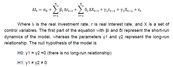

We start by conducting a bounds test for the null hypothesis of no cointegration. The calculated F-statistic is compared with the critical value tabulated by Pesaran and Pesaran (1997), and Pesaran et al. (2001). If the test statistic exceeds the upper critical value, the null hypothesis of a no long-run relationship can be rejected regardless of whether the underlying order of integration of the variables is 0 or 1. Similarly, if the test statistic falls below a lower critical value, the null hypothesis is not rejected. However, if the test statistic falls between these two bounds, the result is inconclusive. When the order of integration of the variables is known and all the variables are I(1), the decision is made based on the upper bound. Similarly, if all the variables are I(0), then the decision is made based on the lower bound.

The ARDL method estimates (p+1)k number of regressions in order to obtain the optimal lag length for each variable, where p is the maximum number of lags to be used and k is the number of variables in the equation. The orders of lags in the ARDL model are selected by either the Akaike Information Criterion (AIC) or Schwartz Bayesian Criterion (SBC), before the selected model is estimated by ordinary least squares (OLS). In the second step, if there is evidence of a long-run relationship (cointegration) among the variables, the following long-run model is estimated,

After ascertaining the evidence of a long-run relationship, the next step involves estimation of error correction model (ECM), which indicates the speed of adjustment back to long-run equilibrium after a short-term disturbance. The standard ECM involves estimating the following equation.

To ascertain the goodness of fit of the ARDL model, diagnostic and stability tests are conducted. The diagnostic test examines the serial correlation, functional form, normality, and heteroscedasticity associated with the model. The structural stability test is generally conducted by employing the cumulative residuals (CUSUM) and the cumulative sum of squares of recursive residuals (CUSUMSQ).

Annex V: Error Correction Model

Model(1)

Model(2)

Model (3)

Annex VI: Model Performance