Press Release RBI Working Paper Series No. 05 Term Premium Spillover from the US to Indian Markets Archana Dilip* Abstract #The paper estimates and analyses term premium in India and makes an assessment of the interconnectedness and transmission of shocks from the US term structure of sovereign bond yields to that of India. The term premium is estimated by decomposing the yield into two components – risk-neutral rate which reflects expectations of future short-term rates; and term premium which captures the investors’ expectations of future central bank policy, inflation and growth shocks. The paper identifies inflation volatility and monetary policy uncertainty as the two important factors influencing term premium in India. Further, empirical findings indicate that the spillover between the US treasury yields and government security yields in India have increased during the sample period from April 2009 to April 2019. The paper also finds that for the long-term yields, the term premium channel is a stronger transmission channel compared with the risk-neutral rates channel. JEL Classification: C32, E43, E44, E58 Keywords: Term premium, risk-neutral rate, affine model, spillover, zero coupon yield curve Introduction Financial markets broadly reflect the views and forecasts of investors on the future direction of an economy. The bond markets, particularly the government securities market, are closely tracked by market regulators and investors as an indicator of prevalent market sentiments. The long-term bond yields also determine the borrowing cost in an economy and, therefore, influence the real economic activity. Thus, it is not surprising that researchers and policymakers have devoted a significant amount of effort to analyse determinants and information content of bond yields. Apart from domestic factors, bond yields are known to be correlated across countries and the co-movement of longer-term yields are known to affect the independence of domestic monetary policy. Many recent studies like Bruno and Shin (2015), Rey (2015) and Georgiadis (2016) suggest that the monetary policy of the United States (US) is a global factor affecting the financial markets. During the global financial crisis, the long-term interest rates rose in many countries and prompted the implementation of unconventional monetary policies. The US Federal Reserve Bank (hereafter US Fed) initiated the large-scale asset purchase programmes (LSAPs), which involved the purchase of longer-term bonds with the objective of lowering their yields by reducing their supply and thereby increasing their prices. In the face of the use of unconventional central bank policies, an understanding of the financial market spillovers is needed as they have the potential to affect the policy implementation of central banks which otherwise target domestic short-term interest rates. Further, in recent times, the decline in government bond yields in advanced economies has resulted in higher investment flows to emerging market economies. Also, as noted by Moore et al. (2013), increased foreign investment supplemented by growth in both liquidity and principal amount in the local currency government bond markets will lead to stronger linkages between the foreign and domestic interest rates through portfolio reallocation between developed and emerging bond markets. In the Indian setup, Patra et al. (2016) have shown that global spillovers dampen time-varying monetary policy transmission in the domestic bond markets. The Expectations Hypothesis, postulated by Fisher (1896), which explains the variations in yields with changes in maturity, posits that long-term interest rates at any maturity can be decomposed into two components: (i) risk-neutral rate; and (ii) term premium. The risk-neutral rates reflect expectations of future short-term rates; term premium, on the other hand, captures the investors’ expectation of future central bank policy, inflation and growth shocks. This paper decomposes the 10-year government security (G-Sec) yield, considering its importance in determining various borrowing and lending rates, into risk-neutral rates and term premia. It is logical to expect that the long-term yields would be driven more by the term premium than the short-term rates. The term premia estimated for most developed countries are highly correlated with each other (Abbritti et al., 2013). Further, according to Albagli et al. (2015), which analysed the spillovers from the US monetary policy to international bond markets, the spillovers work through different channels, with the term premia channel being a predominant channel in the case of emerging economies. Considering the importance of the term premium, this paper attempts to identify the important domestic drivers of term premium so as to better understand the international linkages. The paper then studies the interactions between the decomposed term structure components of the US and India. The rest of the paper is organised into five sections. The next section provides a brief review of the literature on the decomposition of the term structure (commonly referred to as the yield curve) and interactions between the term structures of different countries. The third section discusses the data and outlines the methodology. The fourth section estimates and analyses term structure in India. Section V measures the term structure spillovers from the US to India and discusses the factors responsible for instances of high and low spillovers. The concluding remarks and scope for future research are given in Section VI. II. A Brief Review of the Literature This section reviews the important literature related to term structure decomposition which led to the development of the modern class of no-arbitrage, affine term structure models. The popular models under this class can be divided into the models that are dependent only on yields and those that make use of additional macroeconomic variables. Further, the section reviews the literature related to the spillovers in term structure between different countries. The term premium may be defined as the excess return the investors require for holding longer-dated bonds instead of rolling shorter-dated bonds (Swanson, 2007). The calculation of term premium requires the differentiation of actual yield from the yield based on the expected future path of short-term interest rates. One simple approach to estimate term premium involves the estimation of average expected short rate based on surveys. This method, however, has serious practical challenges due to irregular availability of survey data. The hypothesis, however, was rejected on the basis of strong statistical evidence by Fama and Bliss (1987) and Campbell and Shiller (1991). A major limitation of the hypothesis was the assumption of constancy of premia over time. A new class of models of term structure was introduced which allowed time-varying term premia. The new class of dynamic term structure models, called the no-arbitrage models, became increasingly popular for extracting term premia from the yield curve. According to the no-arbitrage concept, securities with same risk properties should have the same price. The affine term structure models are a popular class of models and assume the bond yields to be a linear combination of the factors that characterise the yield curve. The modern term structure literature uses affine models that represent the dynamics of bond yields over time with simple vector autoregressions. Kopp and Williams (2018) summarised the similarities in the modern models for the estimation of term premium models as: (i) the models are generally Gaussian (which simplifies the computation); (ii) the yields and the risk-free yields are affine functions of some latent variables; (iii) the dimension of the term structure is reduced using statistical techniques; and (iv) the factors are then fed into an intertemporal model like that of a vector autoregressive (VAR) type model. A comprehensive review of the methods available for estimating term premium is provided by Cohen et al. (2018). Duffie and Kan (1996) introduced the dynamic no-arbitrage affine term structure models, in which the yield of any risk-free zero-coupon bond is affine on a set of unobserved latent factors. They assume that the yields at select fixed maturities follow a parametric multivariate Markov diffusion process with stochastic volatility. Duffee (2002) generalised the specification of the market price of risk of Duffie and Kan (1996) and assumed that the yields follow random walks. Dai and Singleton (2002) used specifications of Duffee (2002) and based on theoretical considerations and empirical evidence from US data, showed that some sub-families of affine term structure models explain the historical interest rate behaviour better than the other models. These papers, in general, have used three principal components of yields to explain bond yields. Cochrane and Piazzesi (2005) worked on US data and showed that a relevant fraction of excess returns on bonds can be captured by using only some select factors. Based on these models, other popular models such as those developed by Kim and Wright (2005) and Adrian et al. (2013) emerged. Kim and Wright (2005), (commonly called KW) decomposed the US term structure by incorporating the estimates of future interest rates obtained from Blue Chip Surveys of professional forecasters. In the ACM model, proposed by Adrian, Crump and Moench (Adrian et al., 2013), the principal components of bond yields serve as pricing factors which are actually the weighted sums of yields. The ACM reported a specification with five principal components of zero coupon yields as pricing factors. Joslin et al. (2011) developed a novel canonical Gaussian dynamic term structure model with pricing factors as an observable portfolio of yields and the conditional forecasts of pricing factors being invariant to the imposition of no-arbitrage restrictions. In contrast to the models discussed thus far, another class of models which makes use of macroeconomic variables in addition to the information contained in the bond yields emerged. Ang and Piazzesi (2003) described the term structure as joint dynamics of bond yields and macroeconomic variables in a VAR setup. They used data on inflation and economic growth along with latent variables to examine the effect of macroeconomic variables on the bond prices and the dynamics of the term structure. Rudebusch and Wu (2008) combined a reduced-form New Keynesian model with an affine no-arbitrage model. However, the model does not have the necessary features to match the moments of macroeconomic variables and bond markets. Hördahl and Tristani (2014) included data on nominal and real yields, inflation, economic slack measure (output gap), and survey estimates of future inflation and interest rates. Crump et al. (2018) proposed a parametric model using the estimates for real Gross Domestic Product (GDP) growth, short-term rate and inflation obtained from the surveys of professional forecasters. Wright (2011) used the affine term structure model for ten industrialised countries using data for eighteen years and observed a decline in term premia internationally. Gürkaynak and Wright (2012) provide a comprehensive summary of the analysis of the term structure in the US. While reviewing the linkages in term structures, it is seen that the majority of the literature is based on the US economy. Spencer and Liu (2010) studied the term structure linkages in the US, UK and the Organisation for Economic Co-operation and Development (OECD) countries. Nyholm (2016) studied the spillovers between the US and Euro term structure of interest rates using a new discrete-time, arbitrage-free term structure model. Ceballos et al. (2016) decomposed the long-term interest rates of G7 countries and analysed the transmission of interest rate movements in the US to the economies through the risk-neutral rates and term premium channels. Li et al. (2017) investigated the impact of US long-term interest rates on a select set of emerging and advanced markets. Miyajima et al. (2014) examined the effect of low US term premium on five Asian economies (Indonesia, Korea, Malaysia, the Philippines and Thailand) using a panel VAR model. They found that domestic bond yields and bank credit affect the spillovers. Kearns et al. (2018) studied the spillovers of monetary policy shocks from seven advanced economies to forty-seven advanced and emerging economies to assess the channels of spillover. They found that the exchange rate regimes influence the extent of spillovers and the most important factor affecting interest rate spillovers was financial openness. Iskrev (2018) examined the dynamic relationship between the term premia of the Euro and the US. Sowmya et al. (2016) studied the interconnectedness in the sovereign bond yields of different maturities between developed and Asian countries, including India, by considering the spillovers in the important components of the yield curve, namely level, slope, and curvature. III. Data and Methodology III.1 Data The paper uses daily data on zero coupon yields1. For the US, data on bond yields based on Gürkaynak et al. (2007) are sourced from the website of the US Fed. This data is updated regularly and is maintained on a daily and monthly frequency. For off-the-run bonds, the data is generated using the Nelson-Siegel-Svensson (NSS) methodology (details in Appendix 1), after removing the less liquid bonds and those with irregular trading. The dataset published by the US Fed also provides the parameters of the underlying NSS curve. In India, the Fixed Income Money Market and Derivatives Association of India (FIMMDA)/Financial Benchmarks India Private Limited (FBIL)2 and the Clearing Corporation of India Limited (CCIL) publish daily data on the Zero Coupon Yield Curve (ZCYC). As the data published by FIMMDA/FBIL are mainly used for valuation purposes, the methodology used by them for yield curve generation is different from that employed by CCIL. The former uses the cubic spline methodology and makes use of ‘nodal points’ – the bonds selected based on the number of trades and volume of trades in the previous month. As a result, the yields generated by FIMMDA/FBIL provide a better fit to the benchmark 10-year yield. The CCIL3, like the US Fed, publishes the parameters of the ZCYC based on the NSS model by considering all outright trades above a certain limit and removing outliers. As the CCIL model considers almost all the trades done in a day without basing with the most traded security of the previous month, the yields generated closely follow the generic yields. This paper makes use of daily data on NSS parameters for the US yields (provided by US Fed) and Indian ZCYC (provided by CCIL) for the period from April 2009 to April 2019. Using these parameters, the zero coupon yields are computed for the daily frequency for maturities ranging from 1 month to 120 months at one month interval. The analysis is done using monthly data4. As the US treasury bonds are deemed as safe haven, the movement of the 10-year Indian G-Sec yields and that of the US is given in Chart 1.  III.2 The ACM Model The ACM approach (outlined in detail in Appendix 2), which allows for the decomposition of yield into risk-neutral components and term premia, exploits the forecasting power of excess returns as reported by Cochrane and Piazzesi (2005). ACM models the zero coupon bond yield as a function of a vector of variables Xt, called pricing or risk factors, and is assumed to follow an autoregressive process. Further, the log excess holding return of a bond maturing in n periods is given as: The approach puts restrictions on the important parameters in order to account for the absence of arbitrage opportunities. The ACM makes use of Ordinary Least Squares (OLS) regression and a three-step procedure in order to arrive at the estimates. In the first step, the pricing factors are regressed on their lagged factors as indicated in equation (1). In the next step, the bond returns are regressed on contemporaneous pricing factor innovations (obtained from the first step), the lagged pricing factors and a constant. In the last step, the parameters representing risk premia are obtained through cross-sectional regression of excess returns on the loadings obtained in the second step. The risk-free yield or the average of the expected future short-term interest rate is obtained by setting the risk parameters to zeroes. The time-varying term premium is then obtained as the difference between the model-fitted yield and the risk-free yield. IV. Term Structure Decomposition IV.1 Level, Slope, and Curvature Following Adrian et al. (2013), this paper makes use of the five-factor model where the pricing factors used in the decomposition are the first five principal components of the data on zero coupon yields of 120 months maturities. Although yields can exclusively be explained by the first three pricing factors which essentially represent level, slope, and curvature, Adrian et al. (2013) emphasise that the excess returns are explained mainly by the third, fourth and fifth principal components (Appendix 3 - Table A1). The estimated yield loadings of each latent factor for each maturity are plotted in Chart 2, which represents the responses of the n-month yield to a contemporaneous shock to the respective factor. The first component has positive coefficients and is roughly flat. This can be seen as a proxy for the level. The second component is downward sloping and has positive coefficients at the short-end, neutral at the centre and then negative towards the long-end of the curve. This represents the slope. The third component has positive coefficients at the short-end and long-ends with negative coefficients at the centre and represents flexing of the yield curve. This can be seen as a proxy for curvature. 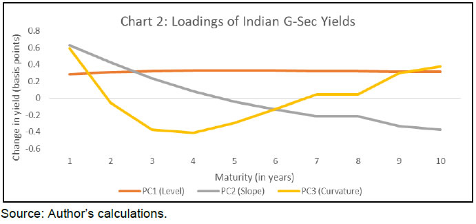 IV.2 Term Premium and Risk Neutral Rate The 10-year bond yield is closely followed by investors and is considered to be an important economic indicator. In the Indian economy, it also serves as a benchmark for other financial transactions and products. The empirical analysis is, therefore, based on the 10-year term premia and the expectations of the short-term rate over the next ten years. Chart 3 plots the decomposition of Indian 10-year bond yield into expectation and term premium components following the methodology explained above. It can be seen that the 10-year yield has tracked the movements in the term premium as the risk-neutral yield remained flat.
| Table 1: Share of term premium in bond yields variations (in per cent) | | Tenure | India Share | US Share | | 1 year | 26.74 | 41.36 | | 5 years | 64.09 | 55.91 | | 10 years | 84.36 | 65.43 | | Source: Author’s calculations. | From Table 1, it can be seen that the term premium on an average, explains only about 27 per cent of the fluctuations in the Indian short-term yields. This implies that around 73 per cent of the variations in the short-term yields are due to changes in expectation of the short rates in the next year. In contrast, the term premium explains around 84 per cent of the fluctuations in the long-term yields. In the case of the US, the share is lower at 65 per cent. These findings are in line with Wright (2011), who finds that in the case of the OECD countries, the fluctuations in long-term yields are overwhelmingly explained by term premium. In the US, the share of term premium in determining the yield changes is much lesser across longer tenures. The co-movement of the 10-year US term premium and that of India is given in Chart 4. As evident from Chart 4, it can be seen that the term premia have declined during the considered period, with the decline appearing prominent during the period from 2013 to 2019. This is consistent with the global downward trend in term premia as observed by Cohen et al. (2018). The decreasing trend in the term premia during 2009–13 ended around the time of the taper tantrum episode of 2013. A higher term premia post the taper tantrum indicates that the long-term interest rates were higher than expected, and the bond market participants were expecting to earn risk premium for holding bonds for a longer term. As noted by Cohen et al. (2018), the comments from the US Fed officials, in conjunction with the purchases made by the US Fed, could have caused the term premia to increase. Post the taper tantrum of 2013, stronger co-movement can be seen between the Indian term premia and the US term premia. The 10-year term premium for the US touched negative values at the beginning of 2015 and has remained in the negative zone since 2017. According to Bernanke (2015), the high level of demand for longer-term bonds could have caused term premiums to become negative. Regulatory policies in the US require insurance companies and pension funds to hold significant amount of safe, longer-term bonds, thereby increasing their demand. As noted by Barnett and Zmitrowicz (2018), if the relative supply of longer-term bonds were to fall, the pension funds become willing to pay a higher price for the bonds (at a lower yield) which can create downward pressure on longer-term bonds. 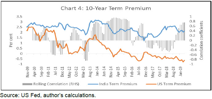 The risk-neutral yields for India remained flat during the period under consideration (Chart 5). India adopted the inflation targeting regime in February 2015 leading to stable average expectations of the short-term rates. This reflects downward revisions of future inflation by the investors. On the other hand, the risk-neutral yields increased in the US in the light of slower than expected output growth and anticipation of policy rate hikes by the US Fed (Chart 5).  As suggested by Bauer et al. (2012), another reason for the stable risk-neutral yields could be the assumption of the short-term interest rates following a VAR(1) process in the estimation of affine models using ACM. In order to account for this criticism, the indirect indifference procedure following Bauer et al. (2012) is used. They showed that due to the small-sample bias, the ordinary least square method generates artificially lower persistence than the true process. This can lead to understating of the volatility of risk-neutral rates, thereby overstating of the volatility of term premium. The mean bias-correction procedure applying the stationary correction technique (Kilian,1998) using 5000 simulations are deployed to obtain the
IV.3 Domestic Drivers of Term Premium This subsection explores the domestic factors determining term premia in India. However, crude oil prices in the international market are considered to be the key variables to influence bond yields globally, due to their implications on inflation and economic activity. The term premia for India and the US are found to be highly correlated with crude oil prices, with the correlation between Indian term premia and Brent crude oil prices being higher at 0.67 (Chart 7). With a view to identifying the domestic drivers of the Indian term premium, the 10-year term premium is regressed on the lagged term premium, the standard deviation of inflation5, lagged net foreign portfolio investments in debt, G-Sec market depth (measured by the average daily turnover of the deals done in the NDS-OM platform6 and over the counter deals), 5-year Overnight Index Swap (OIS) rate, which is considered as a measure of policy rate uncertainty and a constant. | Table 2: Determinants of Term Premium | | Variable | Coefficient | | Term_Premium(-1) | 0.89 *** (15.68) | | ΔAverage_Turnover | -10.91*** (-3.79) | | Sd_Inflation | 0.07***(3.83) | | Δ(OIS5) | 0.22** (1.97) | | FPI(-1) | -0.06***(-3.09) | | c | 0.28** (1.98) | | R-bar2 | 0.87 | | Durbin Watson | 1.96 | | LB-Q (p-value) | 0.73 | ***, **, * represent significance at 1 per cent, 5 per cent and 10 per cent levels, respectively.
Notes:
1. Results of the unit root tests are presented in Appendix 3 - Table A2.
2. Figures in parenthesis are t-statistics based on heteroscedasticity and autocorrelation consistent (HAC) corrected standard errors.
3. LB-Q is p-value of Box-Pierce-Ljung Q-statistic for the null hypothesis of no correlation up to 4 lags.
4.Δ is the difference operator.
5. Average_Turnover = Daily average turnover (per cent of GDP), Sd_Inflation = Rolling-over standard deviation of CPI inflation, OIS5 = 5-year OIS rate, FPI = Net foreign portfolio investments in debt (per cent of GDP). | From the regression results (Table 2), term premium estimates are plausible as the signs of coefficients are in expected lines. The inflation volatility and OIS rates are positively correlated with the term premium, indicating that the investors would demand greater compensation in the face of uncertainty. Turnover, which gives an indication of the liquidity in the G-Sec market, has a negative impact on term premium. Also, the negative coefficient for the net foreign portfolio investments indicate that an increase in foreign investments leads to lower term premia. V. Measuring Spillovers The spillover, which capture the transmission of shocks and interconnectedness between the US and India are estimated using the VAR model’s forecast error variance decomposition following the method suggested by Diebold and Yilmaz (2009). According to this method, for each asset i (i=1,2, … N), the share of its forecast error variance coming from shocks to asset j, are added, and then added across all assets. The shocks are decomposed using Cholesky decomposition. Another variation of this method is the one suggested by the same authors (Diebold and Yilmaz, 2012). The difference in the methodology is that in the latter, the shocks are decomposed using a generalised VAR framework (Pesaran and Shin, 1998), wherein the ordering of the variables included in the VAR does not affect the forecast error variance decompositions. This paper makes use of the method outlined in Diebold and Yilmaz (2009) as the focus is on the spillovers from the US to India. The Diebold and Yilmaz (2009) method of constructing a spillover index is outlined below.  The specified VAR model is found to be (covariance) stationary (Appendix 3 – Chart A1). Based on the Schwarz Information Criterion (SIC), Akaike Information Criteria (AIC) and Hannan-Quinn (HQ) criterion, the optimal lag-length of the VAR model is determined to be one. Using the augmented Dickey–Fuller test, the variables show I(1) order of integration (Appendix 3 – Table A4). Johansen’s cointegration test indicate cointegration between the included variables suggesting that the optimal model would be a mixture of VARs and Vector Error Correction (VEC) models. However, as suggested by Nyholm (2016), the VAR model would suffice considering the fact that the impulse responses for VAR models, which include cointegrated variables, would be unbiased in the case of spillover analysis done for short forecast horizons. 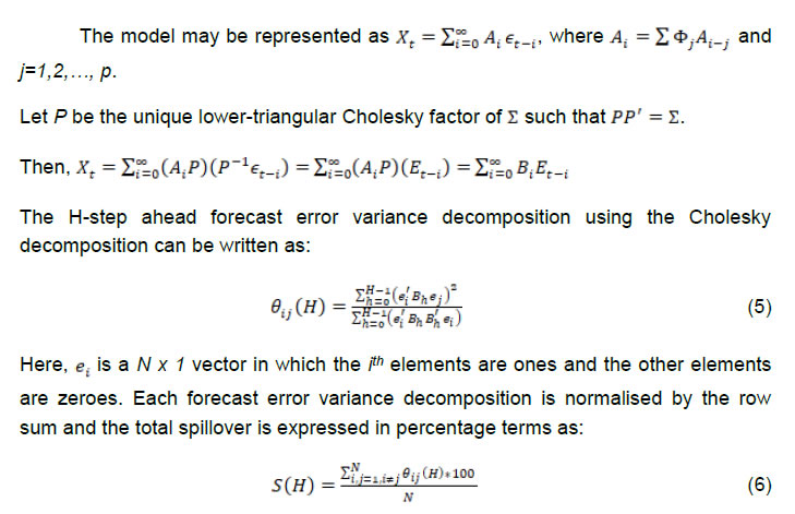 Thus, the spillover index is computed as given in equation (6) as the ratio of the sum of the off-diagonal elements of the matrix (obtained from the variance decomposition exercise) to the total number of variables. One main advantage of using this method is that indices can be designed to track the spillovers between different subsets of the variables in the VAR model. V.1 Results An overall index, which may be viewed as a summary measure to portray the total spillovers between all variables included in the VAR is constructed. The rolling-over spillovers are constructed using a window of 30-months and forecast horizon of 12-months to understand the movement of the spillover during the period of study. The index increased from 45.1 per cent at the beginning of the period to 77.1 per cent in April 2019, indicating increased interaction between the two countries (Chart 8). Also, the spillover pattern has become more volatile following the taper tantrum in 2013.
i) Trade balance: As highlighted by Li et al. (2017), the trade channel is an important channel while studying business cycle synchronisation and spillovers. ii) Net foreign assets: This is a proxy indicator for financial integration. If a country is more financially open, then it is more prone to capital flow reversals. iii) Volatility in the bond market: The Merrill Lynch Option Volatility Estimate (MOVE) Index is a measure of implied volatilities in options on US treasury futures. The index is used as a proxy to measure the volatility in the bond market. It is expected that more volatility would result in spillovers of larger magnitudes. iv) Monetary policy rate: The policy rate, which is mainly driven by the inflation in the country, is another factor that could affect the intensity of spillovers. The results of the estimated regression equation are given in Table 3. The coefficients of the variables are found to be statistically significant and the signs are in line with the expectations. When the country is more financially integrated with the rest of the world and the bond markets are volatile, the spillovers would be stronger. | Table 3: Determinants of Spillover | | Variable | Coefficient | | Overall(-1) | 0.589***(7.58) | | ∆(Net_Foreign_Assets) | 0.003**(2.52) | | MOVE | 0.059**(2.00) | | ∆ (Repo) | -9.24***(-2.88) | | Trade_Balance(-1) | -0.001**(-2.21) | | C | 16.32***(2.80) | | R-bar2 | 0.50 | | Durbin-Watson stat | 2.04 | | LB-Q (p-value) | 0.58 | ***, **, * represent significance at 1 per cent, 5 per cent and 10 per cent levels, respectively.
Notes:
1. Results of the unit root tests are presented in Appendix 3 - Table A3.
2. Figures in parenthesis are t-statistics based on heteroscedasticity and autocorrelation consistent (HAC)-corrected standard errors.
3. LB-Q is p-value of Box-Pierce-Ljung Q-statistic for the null hypothesis of no correlation up to 4 lags.
4. Δ is the difference operator.
5. Overall =Total spillover index, Net_Foreign_Assets = RBI’s net foreign exchange assets in Rs billion, Trade_Balance = Difference between exports and imports in Rs billion, Repo = RBI’s Repo rate. | Based on the total spillover obtained, different spillover indices can be constructed to measure spillovers between different subsets of variables included in equation (4). A subset of the overall spillover index that involves spillover from the US to Indian variables is considered next. The rolling-over spillovers from the US variables to the Indian variables, for a window width of 30-months and forecast horizon of 12-months did not show any monotonic pattern (Chart 9). The spillover from the US variables to the Indian term premium has increased from 37.8 per cent at the beginning of the sample period to 42.6 per cent in April 2019, after witnessing intermittent highs and lows. As in the case of the overall index, the spillovers from the US to India fluctuated within a smaller band during the period from 2010 to 2013, but became more volatile after the taper tantrum. It is observed that the steady increases in the spillover index generally correspond to the US policy rate hikes (as seen in December- 2015, December- 2016, March- 2017, and June- 2018). This is because the rate hikes are expected to lead to rise in yields of US treasury bonds and a stronger US dollar which would subsequently narrow the spread between the US and India yields. This, in turn, would make the Indian bonds less attractive for the foreign investors and the rupee carry trade less profitable. This would lead to increased spillover from the US to India. On the other hand, sudden dips in the spillovers correspond to the initiation of injection of durable liquidity by the Reserve Bank of India (RBI) through the purchase of G-Sec through Open Market Operations (OMO) auctions. This pattern was particularly observable in March 2016 and May 2018. 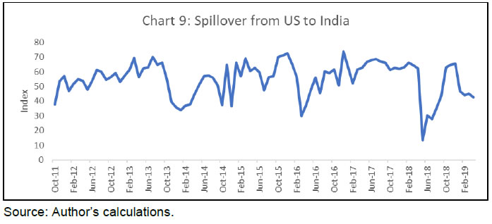 The spillovers from the considered US variables to the Indian 10-year term premium and to that of the Indian 10-year risk-neutral yield are calculated separately. Although no monotonic behaviour was observed in both the indices, it is interesting to note that the spillovers from the US variables to the Indian 10-year term premium was the highest in December 2015, following the announcement of the first policy rate hike since June 2006 by the US Fed. In order to understand the relative strength of the term premium channel and the risk-neutral yield channel, the share of spillovers from the US variables to the Indian term premium and the risk-neutral yields to the total spillovers from the US to India are calculated. During the sample period, the share of spillovers from US variables to the Indian term premium was higher at 65.2 per cent as compared to 34.8 per cent for the risk-neutral yield. Thus, the term premium channel turned out to be the more dominant channel of spillover in the long-term yields. V.2 Robustness Analysis With a view to check for robustness, the analysis is undertaken for two alternate forecast horizons of 10-months and 20-months. As evident from Chart 10, the spillover index is largely robust to the variations done in the forecast horizon. Apart from the maturity, the liquidity of bonds is another major characteristic from the perspective of spillover. In the Indian G-Sec market, the 10-year bonds are the most actively traded and therefore are expected to absorb shocks faster. Therefore, two additional control variables are introduced in equation (4) to account for the impact of differential market liquidities in the Indian and US markets. The average daily volume traded in the 10-year bonds7 are used as proxies for market liquidities. The specified VAR model is found to be (covariance) stationary. Based on the SIC and HQ criteria, the optimal lag-length of the VAR model is determined to be one.  The rolling-over spillovers for a window width of 30-months and forecast horizon of 12-months suggest that the liquidity adjusted spillovers, although lesser in magnitude, have generally tracked the movement of the overall spillovers (Chart 11). Also, the index has generally increased over the sample period indicating increased interaction between the two countries, even after controlling for the liquidity differences. VI. Conclusion The co-movement in long-term yields across countries is a well-known phenomenon. There is, however, lesser understanding of the pattern of movement in the underlying components of yields across countries. Using the ACM methodology, the paper attempted the decomposition of the 10-year G-Sec yield into two components, viz., term premium and risk-neutral yield. The paper also identified important domestic factors that affect the Indian 10-year term premium. The 10-year term premium for India is affected by market liquidity, inflation volatility, monetary policy uncertainty and net foreign portfolio investments. Furthermore, the Indian and US term premia were found to be highly correlated with oil prices. The decline in term premium in India is consistent with the global trend and this indicates the reduced uncertainty about future inflation. Further, stable risk-neutral yields observed after the adoption of the inflation-targeting regime reflect lower expectations of future inflation and the trust of the market that inflation would be contained within the target band. The transmission of shocks and interconnectedness between the US and India have increased over the sample period. This result is robust even after accounting for the difference in market liquidities between the US and India. As expected, the paper finds stronger spillover with increased financial integration and volatile bond markets. The spillovers from the US to India showed upward movements with the US monetary policy rate hikes, while it declined following the announcement of OMO purchase auctions by the RBI. For long-term yields, the share of term premium was much higher than the risk-neutral yields. Also, the term-premium channel was found to be a stronger transmission channel than the risk-free yield channel. Further research on the subject could focus on the spillovers from other important countries.
References Abbritti, M., Dell'Erba, M. S., Moreno, M. A., & Sola, M. S. (2013). Global factors in the term structure of interest rates (No. 13-223). International Monetary Fund. Adrian, T., Crump, R. K., & Moench, E. (2013). Pricing the term structure with linear regressions. Journal of Financial Economics, 110(1), 110-138. Albagli, E., Ceballos, L., Claro, S., & Romero, D. (2015). Channels of US Monetary Policy Spillovers into International Bond Markets. Available at SSRN 2684921. Ang, A., & Piazzesi, M. (2003). A no-arbitrage vector autoregression of term structure dynamics with macroeconomic and latent variables. Journal of Monetary economics, 50(4), 745-787. Barnett, R., & Zmitrowicz, K. (2018). Assessing the Impact of Demand Shocks on the US Term Premium. Bank of Canada. Bauer, M. D., Rudebusch, G. D., & Wu, J. C. (2012). Correcting estimation bias in dynamic term structure models. Journal of Business & Economic Statistics, 30(3), 454-467. Bernanke, B (2015), Why are Interest Rate so Low, Part 4: Term Premium, available at https://www.brookings.edu/blog/ben-bernanke/2015/04/13/why-are-interest-rates-so-low-part-4-term-premiums/ Bruno, V., & Shin, H. S. (2015). Capital flows and the risk-taking channel of monetary policy. Journal of Monetary Economics, 71, 119-132. Callaghan, M. (2019). Expectations and the term premium in New Zealand long-term interest rates (No. AN2019/02). Reserve Bank of New Zealand. Campbell, J. Y., & Shiller, R. J. (1991). Yield spreads and interest rate movements: A bird's eye view. The Review of Economic Studies, 58(3), 495-514. Ceballos, L., Naudon, A., & Romero, D. (2016). Nominal term structure and term premia: evidence from Chile. Applied Economics, 48(29), 2721-2735. Cochrane, J. H., & Piazzesi, M. (2005). Bond risk premia. American Economic Review, 95(1), 138-160. Cohen, B. H., Hördahl, P., & Xia, F. D. (2018). Term premia: models and some stylised facts. BIS Quarterly Review September 2018, 79-91. Crump, R. K., Eusepi, S., & Moench, E. (2018). The term structure of expectations and bond yields. Dai, Q., & Singleton, K. J. (2002). Expectation puzzles, time-varying risk premia, and affine models of the term structure. Journal of financial Economics, 63(3), 415-441. Diebold, F. X., & Yilmaz, K. (2009). Measuring financial asset return and volatility spillovers, with application to global equity markets. The Economic Journal, 119(534), 158-171. Diebold, F. X., & Yilmaz, K. (2012). Better to give than to receive: Predictive directional measurement of volatility spillovers. International Journal of Forecasting, 28(1), 57-66. Duffee, G. R. (2002). Term premia and interest rate forecasts in affine models. The Journal of Finance, 57(1), 405-443. Duffie, D., & Kan, R. (1996). A yield‐factor model of interest rates. Mathematical finance, 6(4), 379-406. Fama, E. F., & Bliss, R. R. (1987). The information in long-maturity forward rates. The American Economic Review, 680-692. Fisher, I. (1896). Appreciation and Interest: A Study of the Influence of Monetary Appreciation and Depreciation on the Rate of Interest with Applications to the Bimetallic Controversy and the Theory of Interest (Vol. 11, No. 4). American economic association. Georgiadis, G. (2016). Determinants of global spillovers from US monetary policy. Journal of International Money and Finance, 67, 41-61. Gürkaynak, R. S., Sack, B., & Wright, J. H. (2007). The US Treasury yield curve: 1961 to the present. Journal of monetary Economics, 54(8), 2291-2304. Gürkaynak, R. S., & Wright, J. H. (2012). Macroeconomics and the term structure. Journal of Economic Literature, 50(2), 331-67. Hördahl, P., & Tristani, O. (2014). Inflation risk premia in the euro area and the United States. International Journal of Central Banking, 10(3), 1-47. Iskrev, N. (2018). Term premia dynamics in the US and Euro Area: who is leading whom?. Economic Bulletin and Financial Stability Report Articles and Banco de Portugal Economic Studies. Joslin, S., Singleton, K. J., & Zhu, H. (2011). A new perspective on Gaussian dynamic term structure models. The Review of Financial Studies, 24(3), 926-970. Kearns, J., Schrimpf, A., & Xia, F. D. (2018). Explaining monetary spillovers: the matrix reloaded. BIS Working Papers No. 757. Kilian, L. (1998). Small-sample confidence intervals for impulse response functions. Review of economics and statistics, 80(2), 218-230. Kim, D. H., & Wright, J. H. (2005). An arbitrage-free three-factor term structure model and the recent behavior of long-term yields and distant-horizon forward rates, FEDS Working Paper No. 2005-33. Kopp, E., & Williams, P. D. (2018). A Macroeconomic Approach to the Term Premium. International Monetary Fund. Li, K. F., Fong, T., & Ho, E. (2017). Term Premium Spillovers from the US to International Markets. HKIMR Working Paper No. 07/2017. Miyajima, K., Mohanty, M. S., & Yetman, J. (2014). Spillovers of US unconventional monetary policy to Asia: the role of long-term interest rates. BIS Working Papers No. 478. Moore, J., Nam, S., Suh, M., & Tepper, A. (2013). Estimating the impacts of US LSAP's on emerging market economies' local currency bond markets (No. 595). Staff Report, Federal Reserve Bank of New York. Nelson, C. R., & Siegel, A. F. (1987). Parsimonious modeling of yield curves. Journal of business, 473-489. Nyholm, K. (2016). US-euro area term structure spillovers, implications for central banks. The European Central Bank Working Paper No.1980. Patra, M. D., Pattanaik, S., John, J., & Behera, H. K. (2016). Monetary Policy Transmission in India: Do Global Spillovers Matter?. RBI Occasional Papers, 37(1). Pesaran, H. H., & Shin, Y. (1998). Generalized impulse response analysis in linear multivariate models. Economics letters, 58(1), 17-29. Rey, H. (2015). Dilemma not trilemma: the global financial cycle and monetary policy independence (No. w21162). National Bureau of Economic Research. Rudebusch, G. D., & Wu, T. (2008). A macro‐finance model of the term structure, monetary policy and the economy. The Economic Journal, 118(530), 906-926. Sowmya, S., Prasanna, K., & Bhaduri, S. (2016). Linkages in the term structure of interest rates across sovereign bond markets. Emerging Markets Review, 27, 118-139. Spencer, P., & Liu, Z. (2010). An open-economy macro-finance model of international interdependence: The OECD, US and the UK. Journal of banking & finance, 34(3), 667-680. Svensson, L. E. (1994). Estimating and interpreting forward interest rates: Sweden 1992-1994 (No. w4871). National bureau of economic research. Swanson, E. T. (2007). What we do and don't know about the term premium. FRBSF Economic Letter. Wright, J. H. (2011). Term premia and inflation uncertainty: Empirical evidence from an international panel dataset. American Economic Review, 101(4), 1514-34.
Appendix 1: Nelson-Siegel Svensson Model The Nelson-Siegel Svensson model (1994) is an extended version of the Nelson and Siegel (NS) functional form (1987) with two additional parameters to be estimated in order to account for one more hump along with the tenors. The NSS model captures the general shape of the yield curve along with the important components like level, slope, curvature, and convexity effectively. The forward rates as per the NSS model are governed by six parameters according to the following functional form as:
Appendix 2: The ACM Model The ACM makes use of ordinary least squares (OLS) regression and a three-step procedure in order to arrive at the estimates. ACM models zero coupon bond yield as function of a vector of variables Xt called pricing or risk factors and is assumed to follow an autoregressive process. At this stage, the returns for the excess holding period can be expressed as a function of the expected return of bonds, a convexity adjustment, the priced shocks to the pricing factors, and an orthogonal return pricing error as:
Appendix 3: Statistical Tests | Table A1: Principal Component Analysis | | Number of Factors | Cumulative Explained Variation | | K=1 | 92.72% | | K=2 | 99.49% | | K=3 | 99.89% | | K=4 | 99.99% | | K=5 | 100.00% | | K=6 | 100.00% |
| Table A2: Determinants of Term Premium-Unit Root Tests | | Null Hypothesis: Variable has a unit root | | Variable Name | Augmented Dickey–Fuller Test | Phillips–Perron Test | Integration | | In Level | | Term_Premium | -5.06 (0.0002) | -4.99 (0.0002) | I(0) | | OIS5 | -2.25 (0.1924) | -2.25 (0.1923) | I(1) | | Average_Turnover | -2.66 (0.0906) | -2.56 (0.1093) | I(1) | | Sd_Inflation | -5.32 (0.0001) | -5.26 (0.0001) | I(0) | | FDI | -3.91(0.0045) | -3.92(0.0045) | I(0) | | In First Difference | | OIS5 | -5.83(0.0000) | -5.83(0.0000) | I(0) | | Average_Turnover | -6.75 (0.0000) | -12.65 (0.0000) | I(0) | | p-value in parentheses |
| Table A3: Determinants of Spillover–Unit Root Tests | | Null Hypothesis: Variable has a unit root | | Variable Name | Augmented Dickey–Fuller Test | Phillips–Perron Test | Integration | | In Level | | | Overall | -4.57 (0.0003) | -4.61 (0.0002) | I(0) | | Net_Foreign_Assets | -0.26 (0.9253) | -0.25 (0.9274) | I(1) | | MOVE | -3.49 (0.0102) | -3.29 (0.0183) | I(0) | | Repo | -1.76 (0.3970) | -2.22 (0.2004) | I(1) | | Trade_Balance | -4.06 (0.0017) | -3.96 (0.0024) | I(0) | | In First Difference | | | Net_Foreign_Assets | -8.84 (0.0000) | -8.73 (0.0000) | I(0) | | Repo | -9.06 (0.0000) | -9.69 (0.0000) | I(0) | | p-value in parentheses |
| Table A4: VAR Model for Spillover Index–Unit Root Tests | | Null Hypothesis: Variable has a unit root | | Variable Name | Augmented Dickey–Fuller Test | Phillips–Perron Test | Integration | | In Level | | 10-year US Term Premium | -1.36 (0.6015) | -1.41(0.5734) | I(1) | | 10-year Indian Term Premium | -2.56 (0.1043) | -2.76( 0.0674) | I(1) | | 10-year US Risk-neutral Yield | -0.15 (0.9405) | 0.14 (0.9676) | I(1) | | 10-year Indian Risk-neutral Yield | -2.55 (0.1059) | -2.66 (0.0850) | I(1) | | USD/INR | -0.83 (0.8060) | -0.55 (0.8771) | I(1) | | In First Difference | | 10-year US Term Premium | -9.95 (0.0000) | -9.95 (0.0000) | I(0) | | 10-year Indian Term Premium | -10.72 (0.0000) | -10.72 (0.0000) | I(0) | | 10-year US Risk-neutral Yield | -12.89(0.0000) | -12.90 (0.0000) | I(0) | | 10-year Indian Risk-neutral Yield | -9.12(0.0000) | -9.03 (0.0000) | I(0) | | USD/INR | -8.32(0.0000) | -8.08 (0.0000) | I(0) | | p-value in parentheses |
If the VAR is (covariance) stationary, then all AR roots should lie within the unit circle. |