Press Release RBI Working Paper Series No. 01 Monetary Policy Transmission in India:
New Evidence from Firm-Bank Matched Data Saurabh Ghosh, Abhinav Narayanan and Pranav Garg@ Abstract *This paper uses a unique firm-bank matched data set for India to provide new insights into the monetary policy transmission mechanism. We first show that monetary policy transmission works with a lag when we focus on bank credit and balance sheet items of firms. An assessment of the bank-lending channel suggests that an increase in credit may have a heterogeneous effect on firms based on the liquidity positions of the lending banks. Investment in fixed assets is found to increase for firms that borrow from liquid banks, when these banks increase their lending. By contrast, we find increased financing of current liabilities - and not increase in long-term investment - for firms that borrow from the less liquid banks. The paper highlights the importance of term spread, liquidity position and strength of the balance sheet of banks for effective transmission of monetary policy. JEL Classification: C58, E44, E52 Keywords: Monetary policy, transmission, firm-bank matched data Introduction Monetary policy transmission is the process through which policy action of the central bank is transmitted to meet the ultimate objectives of inflation and growth. In general, policy transmission is considered to be a two-stage process. In the first stage, the policy shock impacts different segments of the financial markets. In the second stage, it gets transmitted to the real economy (Mishkin, 2012). The policy transmission mechanism hinges crucially on how changes in monetary policy affect household, firm and bank behaviours. While households and firms are on the demand side, banks supply credit and facilitate efficient resource allocation. In this paper, we analyse how monetary policy shocks are transmitted to the banks and, in turn, are transmitted to the firms. We use unique firm-bank matched data to understand the mechanisms of monetary policy transmission by exploiting bank heterogeneity (in terms of liquidity) and firm heterogeneity (in terms of leverage).1 First, we examine how policy rate changes affect the bank balance sheet, especially through the lending channel. Second, we analyse how changes in policy rate affect firms’ balance sheets through their debt structure. Finally, we look at how the balance sheets of banks affect the investment decisions of the firms to which the banks lend. We exploit the heterogeneity of the banks in terms of their liquidity position to comment on whether more liquid banks induce a better transmission mechanism. Additionally, we comment on whether more leveraged firms respond quickly to bank balance sheet changes relative to less leveraged firms. An important assumption behind an effective transmission mechanism is that firms’ and banks’ balance sheets are strong. These conditions enable the agents to react quickly and optimally to policy changes (Acharya, 2017). If these assumptions are violated, then monetary policy may be less effective and can operate with long and variable lags. Literature has identified several channels through which the transmission of policy rates to operational targets takes place (Bernanke and Gertler, 1995; Gertler and Gilchrist, 1994; Kashyap and Stein, 2000; Romer and Romer, 1989). The most important among them are: (i) interest rate channel, (ii) credit channel, (iii) exchange rate channel, and (iv) asset price channel. Over the past few decades, academic literature has concentrated on three primary challenges relating to monetary policy transmission: (a) identifying the transmission channel(s); (b) identifying demand-side (firm, household) and supply-side (banks) frictions that dampen transmission; and (c) estimating long and variable lags. The first identification is perhaps the most challenging as some of the transmission channels work simultaneously instead of working in isolation. To understand the underlying mechanisms, we must study the reasons for the heterogeneity in bank-level responses to changes in monetary policy. In this vein, it may be useful to identify some of the frictions affecting bank-specific transmission and the large body of empirical work that has attempted to address most bank-specific factors (bank size, liquidity and market capitalisation) (Bolton et al., 2016; Khwaja and Mian, 2005) on credit response to monetary policy change. In the Indian context, Acharya (2017) noted some frictions (asset quality concerns, expected loan losses in credit portfolios and rigidity in lending rates) relating to a bank’s balance sheet as banks attempt to remain profitable by protecting their net interest margin. Rigidities on the liability side of banks’ balance sheets, which dampen effective policy transmission include fixed interest rate on bulk of deposits and high returns in other forms of financial savings (e.g. mutual funds, post office deposits, etc.). Therefore, banks must compete with alternative financial savings, which makes it difficult for them to change their deposit rates in consonance with policy rate signals, particularly during the easing cycle of monetary policy. Moreover, regulatory capital requirements, loan risk weights and balance sheet stress make banks risk averse, therefore reducing the supply of bank credit to risky sectors. Popov (2016) finds that easy monetary conditions increase bank credit in general and to ex- ante risky firms, especially by banks with lower capital ratios. With regard to the impact of monetary policy transmission on investment demand, a large number of studies have analysed firm-level panel data to study the factors influencing rate transmission. Chetty and Szeidl (2007) found evidence of demand-driven transmission that works through firms’ creditworthiness (balance sheets), and is independent of the bank-lending channel. Jiménez et al. (2017) analysed the role of balance sheet strength in influencing credit availability and underlined the importance of the strength of corporate balance sheets to enhanced credit availability of firms. While there has been considerable research on the conventional views of monetary policy transmission, separating demand shocks, which affect firms’ demand for credit, from supply shocks, which impact banks in their credit creation, is a relatively new area of research. A handful of studies have attempted to address this question using a sample of matched firm-bank level data, information on relationship banking, and exogenous shocks. Amiti and Weinstein (2018), using a vast sample of Japanese bank-firm lending data, showed that granular bank supply shocks explain 30 to 40 per cent of aggregate loans and investment fluctuations. Bottero et al. (2015), using bank-firm credit data for Italy, found that shocks to the sovereign bond market led to a drop-in bank lending to corporations, which in turn led to a decline in investment by smaller firms. Chodorow-Reich (2014) used the Lehman Brothers crisis as an exogenous shock and found that lenders’ health has a significant effect on employment at small and medium firms. For India, Bhardwaj et al. (2017), using a sample of bank-dependent firms, found that firms that enjoy an exclusive banking relationship are less susceptible to monetary policy shocks compared to their transactional banking counterparts. Another study (Ghosh, 2007) suggests that a close loan relationship of a firm with a few banks could result in reduced interest cost in India. However, we haven’t come across any study on India that explicitly analyses the interaction of firm-bank balance sheet data for the universe of corporate loans, preferred banking relationships, monetary policy transmission and external shocks. Our paper closely relates to this strand of literature as we have used firm-bank matched data for the universe of corporate loans to identify the bank-to-firm transmission mechanism. It is important to mention here that due to the limitation of firm-bank linked data for Indian firms, we do not have a clean identification strategy like in the studies mentioned above for other countries. In this paper, we look at monetary policy transmission through bank and firm balance sheets. Our first stage results on the impact of monetary policy changes on a bank’s balance sheet suggest a lagged response from the banks. In the second stage of our analysis, we examine the direct effect of monetary policy changes on the balance sheets of firms. We argue that these direct effects may not reflect the true effect of transmission. This is because firms’ investment decisions may be correlated with demand conditions in the economy. In addition, these decisions may depend on the lending decisions of the banks to which the firms are attached. In the third stage, using novel firm-bank matched data, we find that an increase in credit has a heterogeneous effect on firms based on the liquidity of their creditor institutions, unveiling a disguised mechanism at play behind policy transmission in India. Investments in fixed assets increase for firms that are attached to relatively more liquid banks when these banks increase their lending. By contrast, firms borrowing from the least liquid banks exhibit an increase in short-term capital in response to bank lending, presumably because less liquid banks cannot take on as much credit risk. In both cases, highly leveraged firms do not have differential outcomes, indicating that the balance sheet channel is weak. The rest of the paper is structured as follows: Section II presents India’s monetary policy and corporate finance background, Section III discusses the data, Section IV elaborates on the identification strategy and empirical equations used in our model, Section V presents our findings, and Section VI concludes the paper. II. Monetary Policy and Corporate Finance Landscape in India In the Indian context, Das (2020) has identified seven regimes of India’s monetary policy: the initial phase, the synchronisation of monetary policy with the Five-Year Plans, credit planning, monetary targeting, multiple indicator approach, precondition set for inflation targeting, and flexible inflation targeting. The last three phases mark the transition from direct instruments to indirect instruments (e.g. interest rates and transmission channels start gaining importance). In the context of transmission, there is general consensus that policy transmission is fast in the financial markets (ECB, 2011). Money and bond markets react almost instantaneously to changes in policy rate. Transmission to other segments, however, depends on the level of market development, institutional set-up, and liquidity in the underlying segments. Prabu and Ray (2019) attempt to identify the impact of shocks on financial variables. They divided the sample period into three sub-periods, and their results indicate that the impact varies in different segments of financial markets. While the impact is fast and efficient in money and bond markets, rate transmission is relatively limited in foreign exchange and stock markets. Prabhu and Ray also found that the transmission depends on operating procedure and monetary policy stance. In the second stage, among transmission channels, the interest rate channel is found to be significant in most advanced economies (AEs). A bank’s lending (credit) channel, on the other hand, plays an important role in bank-dominated emerging market economies (EMEs). It is predominantly operational in those economies where the central banks have direct control on bank lending (Barran et al., 1996). External finance premium plays an important role for the interest rate and credit channels of transmission. In theory, the direct effects of monetary policy are amplified by endogenous changes in the external finance premium. The size of the external finance premium reflects imperfections in the credit markets that drive a wedge between the expected return received by lenders and the costs faced by potential borrowers. Credit market participants, therefore, internalise monetary policy changes differently, based on their individual balance sheet positions.2 Several studies have attempted to identify the most important monetary policy transmission channel for India. Aleem (2010) estimated a set of vector autoregressive (VAR) models to examine the relative significance of three transmission channels in India. This study suggests that the bank-lending channel plays a pivotal role in rate transmission in India. Bhoi et al. (2017) used time series data and a VAR framework to analyse the responses of a policy shock to the operating target. Their analyses used an innovative technique, the “shutdown methodology” that assigned zero coefficient restriction to certain variables in the output-inflation equation for effective identification. Their study indicates that the interest rate channel of transmission was most dominant in India during the sample period. In this context, Cecchetti (1995) found that credit is affected on the supply side by the balance sheet strength of the banks (the so-called bank-lending channel) and on the demand side by the balance sheet strength of the firms (the so-called firm balance sheet channel). In the Indian context, Prasad and Ghosh (2005) analysed the relationship between monetary policy and corporate behaviour in India and found evidence of strengthening of the interest rate channel operating through corporate investment after 1998. Ghosh and Ghosh (2006), on the other hand, found that monetary policy contraction especially reduces investment of highly leveraged firms. Regarding other transmission channels, Prabu and Ray (2019), Aleem (2010), and the Reserve Bank of India (RBI) (2014) indicate that direct transmission through exchange rate and asset price channels in India has been generally muted, though both factors could have influenced demand creation indirectly. In 1994, RBI deregulated lending rates, and banks were required to declare Prime Lending Rates (PLR). But PLR turned out to be rigid and inflexible in relation to the overall lending rate which led to the introduction of Benchmark PLR (BPLR). This regime was also marked with limited transmission success, as banks were often lending at sub-BPLR rates. As a corrective practice, RBI introduced a base rate system in 2010 based on the cost of borrowing. However, the transmission through base rate turned out to be weak primarily because of banks’ spread adjustments. To improve transmission, a marginal cost-based lending system (MCLR) was introduced in India in 2016, and was further refined by linking all new floating rate personal or retail loans (housing, auto, etc.) and floating rate loans to micro and small enterprises extended by banks to external benchmarks since October 2019. However, some evidence suggests that the MCLR action has not been fully transmitted to corporate borrowings, and there was evidence of long and variable lags. In this regard, RBI (2014) notes that transmission lags vary from one to fourteen quarters for output for a gamut of countries—42 months in the case of the United States (US) and 48 months for the euro area. For India, Bhoi et al. (2017) found that the maximum impulse in gross domestic product (GDP) growth occurs with a lag of two to three quarters. Inflation, on the other hand, reacts with a lag of three to four quarters. Acharya (2017) notes that monetary policy actions are felt with a lag of two to three quarters on output and three to four quarters on inflation, and the impact persists for eight to twelve quarters. III. Data We have compiled four separate pieces of information to construct a novel data set for our analyses: monetary policy rates and spreads (liquidity spread and term spread), bank balance sheet data, firm balance sheet data, and data on lending relationships of firms. These data are combined mainly from two sources, described below. III.1 Database on Indian Economy Data on policy rates and spreads, as well as detailed information on assets and liabilities, profit and loss, and key ratios of Scheduled Commercial Banks (SCBs) in India are publicly available on RBI’s Database on Indian Economy. Balance sheet data are reported annually from 2005 through various statutory returns submitted to the RBI at the level of individual banks.3 The assets and liabilities statement reports 74 variables and the profit and loss account reports 33 variables. An additional 34 key ratios are reported that reflect the financial health of banks. Variables are reported in Rs. 10 Crore or one million in the balance sheets. Broadly, our sample contains all SCBs active in India between FY2005 and FY2019. Chart 1 shows that bank group-wise levels and shares of lending in India’s credit market over the sample period. We find that: (i) nationalised banks have the largest share of credit supply in the Indian market; (ii) the fall in the share of lending by nationalised banks since 2012 has been largely captured by private sector banks; (iii) the share of foreign banks in the Indian market has steadily reduced since 2008. 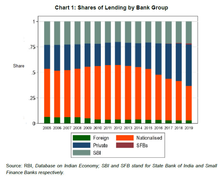 We consider policy rates and spreads that are important in the transmission of monetary policy. Repo rate and reverse repo rate series are available at a weekly frequency from April 2001. Bank rate, Cash Reserve Ratio (CRR) and Statutory Liquidity Ratio (SLR) series are available at a weekly frequency from June 1973. Mumbai Interbank Offered Rate (MIBOR) series is available at a daily frequency from December 1998. Weighted average call rate (WACR) series is provided at a monthly frequency from April 1991. Data on Treasury bill (T-bill) yields is available at a monthly frequency from April 1996. We obtain annual aggregates of policy rates by taking an unweighted average. Policy rate data is then matched with balance sheet data for each fiscal year, e.g. 2019 is April 2018 to March 2019, since balance sheet data is recorded over the fiscal year. Charts 2 to 4 plot the rates and spreads that we utilise as key policy instruments for transmission. These policy instruments include changes in the repo rate, CRR, three-month MIBOR, liquidity premium (Spread 1) and term premium (Spread 2). The repo rate is the most conventional instrument in a central bank’s toolkit, including the Reserve Bank of India. The CRR is a certain percentage of bank deposits which banks are required to keep with the Reserve Bank in the form of reserves or balances. The three-month MIBOR is included to incorporate the changes in a market benchmark. Spread 1, in our paper, is the difference between the WACR (interbank call rate) and the policy repo rate, and is likely to represent the liquidity stance of the central bank (accommodative vs deficit). Finally, Spread 2, the difference between long-term and short-term yields on G-Secs, is calculated to capture term premium. The recent measures of some central banks are intended to improve transmission by influencing the term premium. We intend to evaluate the impact of both term spread and liquidity spread on policy transmission using firm-bank matched dataset. 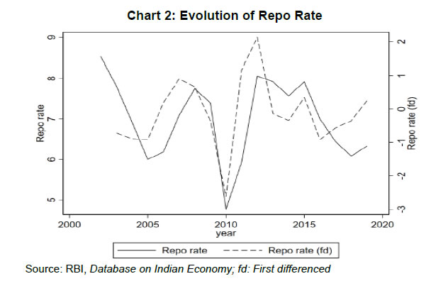 We notice a drop of 300 basis points in the repo rate between 2009 and 2010 in Chart 2. This corresponds with policy intervention to prevent a liquidity shortage in the aftermath of the GFC. CRR conforms well to the macro-prudential outlook of the RBI, showing an upswing between 2005 and 2009, subsequent to which it witnessed a steady decline. The three-month MIBOR responds in a similar manner to the repo rate, with a drop of around 450 basis points. Chart 3 plots the evolution of WACR - Repo rate, which provides a measure of credit market liquidity, with a tightening in liquidity reflected in a rise in the spread. We find that credit markets witnessed a transient liquidity shortage during the GFC (2009–10), as well as for a sustained period from 2011 to 2015. The rise of around 300 basis points in the term spread in Chart 4 is caused by a fall in the 91-day T-bill yield relative to the 10-year benchmark T-bill yield.
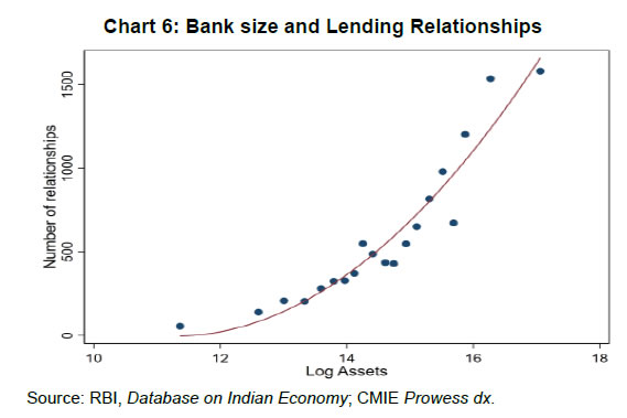
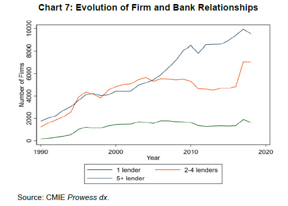
III.2 CMIE Prowess dx Firms’ annual financial statement data are maintained by CMIE Prowess dx4, a popular data source for financial accounts analysis in corporate finance literature on India. The database covers the profit and loss statements, balance sheets, and ratios based on over 40,000 Indian companies since 1990. Variables are reported in INR million in the balance sheets. Prowess includes listed companies, unlisted public companies and private companies across industries and ownership groups. The database comprises: (a) firms that are listed, and (b) unlisted public limited companies that have sales or assets exceeding INR 200,000,000. Firms that are included in Prowess are required to file annual accounting reports and have submitted reports for at least three years. Our analysis focuses on standalone firms versus consolidated entities.5 The banker information contains creditor relationship data for 18,953 firms. Perhaps the most unique feature of this data set is the relationship-based banking practised by Indian firms. CMIE Prowess dx provides data on the banks that the firms borrowed from in a particular year. This database is an exhaustive list of creditor institutions (listed as banker0, banker1, banker2… banker40, and so on) for each firm. This information is available for each firm at an annual frequency. While the order of bank relationships reported might be based on the priority of the relationships, CMIE maintains that this reporting is dependent upon the firm’s discretion and how they want to report lenders, which could be alphabetical, oldest to newest, by credit volume (i.e. prime lender), or random.6 Notably, the creditor institutions include both SCBs as well as non-banking financial companies (NBFCs), cooperative banks and other financial institutions. We use this information to create an annual register for every firm by matching SCBs in the RBI database with lenders for each firm in Prowess. While doing this, we ensure that subsidiary bankers in the Prowess list are matched with parent banks listed in the RBI database through extensive manual matching in cases of merger and acquisition (M&A) histories and changes in identifiers/names over time. Such bank M&A activity is tractable due to the number of SCBs in India (90–95). In this manner, we successfully match 95.1 per cent of lenders from the Prowess data set with detailed bank balance sheet data for those SCBs in the RBI database. We have dropped the remaining 5 per cent of lender relationships from our sample, which are mostly cooperative banks and other NBFCs. We have also excluded firms in agriculture, mining and public utilities. Finally, we have dropped financial sector firms from our sample. In doing so, we dropped an additional 22 per cent of the firm sample. We exclude these firms because the high leverage that is normal for these firms probably does not have the same meaning as for non-financial firms, where high leverage more likely indicates distress. Our final sample consists of both listed and unlisted firms matched with all creditor SCBs for each fiscal year between 2005 and 2019. Our sample has 15.56 per cent firms that are listed. The final set of 12,364 firms are selected to focus on transmission after explicitly accounting for bank-firm relationship. Table A2 in Appendix A details the coverage of firms by NIC-2 sectors in the final panel. IV. Identification Strategy and Empirical Specifications IV.1 Variable Construction and Identification Our main objective is to identify the monetary policy transmission mechanism to the real economy. We approach this identification problem in three steps. First, we study the effect of changes in policy rates and spreads on the growth of key banking variables. Our variables of interest include term loans and liquidity. Term loans provide the first-order evidence of an increase (decrease) in lending due to a change in policy, which would directly establish the bank-lending channel. We define liquidity as the sum of cash in hand, investment in G-Secs and other approved securities normalised by total assets of the bank. Liquidity gives us a sense of how promptly banks may mobilise their liquid funds in response to monetary policy changes. These variables are intricately related to the bank-lending channel. In the second stage, we investigate whether monetary policy directly impacts firms’ short-term (current) and long-term (investment) borrowings, i.e. the demand side. This is the balance sheet channel wherein an increase in policy rate can directly affect firms’ balance sheets by increasing their liabilities through interest payments, thereby adversely affecting their capacity to invest. Specifically, at this stage, we test whether dependence on external finance impacts the way firms internalise policy changes. We include leverage ratio measured by debt-equity ratio to include firms’ dependence on external finance. There are two channels through which monetary policy gets transmitted to the real economy: bank-lending and balance sheet channels. A study of both channels would require information on the exact amount of loans made by each bank to every firm, which, to our knowledge, is not available in India. In this vein, we create a novel database matching our firm-level database with a bank-level database through comprehensive identification of bankers of each firm in each year, accounting for subsidiaries, mergers and acquisitions at the bank level. We are then able to use bank balance sheets specific to each firm-year to determine whether bank-level heterogeneity plays a role in the transmission of policy changes to borrowers. Ideally, a change in the policy rate may have a differential effect on bank lending based on the liquidity positions of the respective banks. The firms that are borrowing from these liquid banks, which are more likely to increase lending may respond positively relative to the firms that are attached to less liquid banks. On the other hand, banks may lend favourably to firms that have low leverage ratios via the balance sheet channel. We rely on an analysis of aggregate lending for each bank, i.e. a bank × year variable. In essence, this means that any result driven by the bank-lending channel is not exclusive to a single firm, but to all firms for whom that bank is a lender. Provided that there is heterogeneity in lenders across firms and in the balance sheet of lenders, we can reach similar conclusions at the first-order. For example, imagine a small credit market with two lenders (banks A and B) and four firms (firms 1 to 4). Identification in our paper comes from the difference in the financial fundamentals of banks A and B, as well as from the fact that some firms, say firms 1 and 2, are matched with bank A as their lender, while other firms, say firms 3 and 4, are matched with bank B. Due to this, we can identify the presence of a bank-lending channel from banks to sub-groups of firms that share those banks as their lenders (i.e. transmission from bank A to all firms that share bank A as their lender i.e. firms 1 and 2). For identification at a bank × firm level, we interact characteristics of lenders with leverage ratios of individual firms. In essence, this allows us to identify whether, in response to a change in monetary policy, firm 1’s decision to increase (decrease) investment is driven by its lender’s response to a policy change or through its own leverage ratio, or through an interaction of both these channels. We argue that when faced with a monetary policy shock liquidity ratio of a bank influences its credit creation. Consider two banks that are similar in all regards except liquidity. The first bank maintains a low buffer of liquid assets such as cash in hand or approved securities, while the second bank holds a higher liquidity ratio. A contractionary policy shock, ceteris paribus, will cause both banks to face a higher cost of capital and will force them to adjust the assets side of their balance sheets. Such adjustment and reallocation could be more for the first bank that held a lower ratio of liquid assets. The more liquid bank, on the other hand would be less stressed by a contractionary monetary policy, and would be relatively comfortable with issuing credit for longer-term investment purposes (Bech and Keister (2012)). In order to distinguish such a channel at the bank level, we separately study transmission for the most and least liquid lenders in the corporate credit market. A firm may have multiple lenders and each lender will lend to multiple firms. For each firm, and in each year, we identify lenders with the most and least liquid balance sheets—out of all other lenders for that firm in that year. Then, we create two sub-panels: firms attached to most liquid and least liquid lenders. Incorporating the entire list of SCBs (and not an arbitrary subset) for each firm is essential for proper identification. Chart 5 plots the density of the number of SCB relationships in our sample.7 It is important to highlight that majority of the firms have multiple banking relationships. Chart 6 & 7 plot the evolution of lending relationships (with all financial intermediaries, inclusive of NBFCs/shadow banks) over our sample period. We find that the number of firms with multiple banking (SCB, NBFCs, shadow banking) relationships has grown substantially between 2002 and 2007, with a brief decline after the GFC, whereas the number of firms with single banking relationships has remained stable. A similar trend holds for only SCB relationships.8 We provide the definition and the source of each variable used in our regression analyses in Table A.1 in Appendix A. All our specifications are in growth terms. Table 1 summarises the information on the key variables that we use in our specifications.9 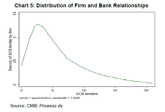
| Table 1: Descriptive Statistics for Key Variables | | Variables | N | Mean | Std. Dev. | 25th perc. | 50th perc. | 75th perc. | 90th perc. | | Policy Rates & Spreads (first diff.) | | Repo Rate | 206,686 | -0.0777 | 1.062 | -0.563 | -0.344 | 0.667 | 1.167 | | 3-month MIBOR | 206,686 | 0.0572 | 1.701 | -0.607 | 0.0608 | 1.172 | 2.298 | | CRR | 206,686 | -0.0511 | 0.808 | -0.156 | 0 | 0.208 | 0.854 | | WACR–Repo | 206,686 | 0.124 | 0.897 | -0.173 | 0.0489 | 0.763 | 1.433 | | 10Y-91D G-Sec | 206,686 | 0.0383 | 1.155 | -0.312 | 0.0377 | 0.355 | 0.625 | | Firm (% change, winsorized at 5%) | | Net Cash Flow from operating activities | 165,016 | -32.22 | 172.1 | -101.3 | -30.82 | 38.61 | 150 | | Sales | 179,647 | 15.28 | 34.90 | -2.201 | 10.67 | 26.52 | 52.04 | | Current Liabilities | 188,980 | 25.96 | 57.76 | -4.383 | 12.17 | 37.45 | 85.88 | | Leverage Ratio (D/E) | 188,559 | 8.802 | 29.93 | -4.904 | 6.419 | 21.11 | 42.86 | | CapEx (total capital) | 49,510 | -45.11 | 116.5 | -100 | -100 | -38.75 | 71.57 | | Bank (% change, winsorized at 5%) | | Liquidity | 192,867 | -1.167 | 11.54 | -7.799 | -2.394 | 5.160 | 15.18 | | Term Loans (non-banking, within India) | 193,077 | 18.41 | 17.75 | 8.239 | 17.31 | 27.81 | 38.65 | | Reference Rate (first diff.) | 191,523 | -0.253 | 1.835 | -0.575 | -0.0625 | 0.500 | 1.375 | | Source: RBI, Database of Indian Economy; CMIE Prowess dx. | IV.2 Empirical Specifications The objective of our empirical analyses is to highlight the transmission mechanism of monetary policy through the bank-lending channel. The transmission mechanism of monetary policy can be broken down in three steps. First, we identify the bank-lending channel by showing that monetary policy has a heterogeneous effect on lending institutions, namely banks. Second, a change in monetary policy may directly affect the firms by changing the liabilities side of the firm’s balance sheet. Specifically, the existing liabilities may change as a response to a change in monetary policy. 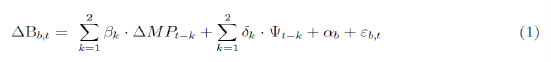 Third, we try and exploit the relationship-lending channel of policy transmission. Specifically, a change in monetary policy may affect the banks’ balance sheet differently based on the liquidity positions of the banks. Thus, a change in monetary policy may have a differential effect on firms based on the particular set of banks that the firms are attached to. In order to investigate whether banks respond to monetary policy changes, we run the following specification at the bank level: 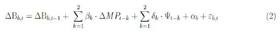 where ΔBb,t is the percentage change in key balance sheet elements for bank b in year t (winsorized at 5 per cent).10 We focus primarily on term loans and liquidity on the assets side of banks’ balance sheets. We also look at the first-difference of reference rate at the bank level, which is defined as BPLR (till 2010), Base Rate (between 2010 and 2016), and MCLR (post 2016). ΔMPt is the difference between t and t − 1 of policy variables. Ψt is a control for macroeconomic conditions, specified as percentage growth in Gross Value Added (GVA) between t and t − 1. αb controls for bank-level unobserved characteristics that influence the evolution of balance sheet elements for individual banks. One concern that may arise while using the above specification is the stickiness of the bank balance sheet variables. Specifically, the balance sheet items may be driven by own past values, in which case the coefficients may be biased. However, balance sheet items may be sticky in levels and less likely to be so in changes (growth rates). Nonetheless, to allay this concern, we run a dynamic panel specification of the following form using generalised method of moments (GMM) techniques:11 Second, we look at whether changes in monetary policy affect growth in investment and current liabilities through firms’ leverage ratio using the following specification: 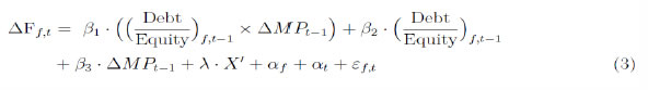 where ΔFf,t denotes growth in firms’ capital expenditure and current liabilities (winsorized at 5 per cent), denoting growth in investment in fixed assets and in short-term capital, respectively. We include ΔMPt−1 which is the lagged growth monetary policy instrument and (Debt/Equity)f.t-1 which is the one-year lagged growth in leverage ratio. We interact the policy instrument and the leverage ratio to tease out the effect of a change in monetary policy on the capital expenditure of the firm with high or low leverage ratio. We also include growth in two firm-specific controls (X') in our model (suppressing subscripts): growth in cash flows and growth in net sales, both in lag terms. The control variables are chosen based on the literature that studies that have studied the lagged effects of monetary policy on firms’ activities (Romer and Romer, 1989). In the above specification, αt captures the cyclical factors that have common effects on all firms, and αf accounts for unobserved firm-specific effects. The main coefficient of interest is β1 which tells us whether the responses of firms to a change in monetary policy are different based on the leverage ratio of the firms. We cluster the standard errors at the firm level. Once again, like in the first stage, we also run a dynamic panel specification to account for stickiness in firm-level variables. We use the following specification: 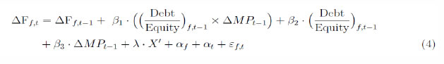 Equations 2 and 4 show the impact of monetary policy on banks and firms, respectively, but are not sufficient to comment on transmission via banks to firms. This could be because banks, on average, respond to monetary policy changes that may be confounded with demand-side factors, in which case identification of the shock (policy change) becomes difficult. On the other hand, firms may increase their investments due to demand-side factors and such an exercise may overlap with a monetary policy easing cycle. Thus, although we may observe a response from banks and firms to a change in monetary policy, these changes could show some correlations which may not purely be driven by policy changes. We know that the ultimate objective of a change in monetary policy is to nudge investments in a positive or a negative way depending on the easing or tightening cycle, respectively. Thus, we need to identify how firms respond to a change in policy and this response must not conflate with any other factors that may affect firm investment. In order to do this, we adopt the following empirical strategy. We first match the firms to their set of lenders. Note that a firm may have multiple lenders and each lender will lend to multiple firms. This variation in lender and firms is central to our identification strategy (see Table 1 for the distribution of bank-level and firm-level variables). This is because lenders react differently to a change in policy and these lenders are attached to different firms. Thus, a firm attached to a lender that responds quickly to a change in monetary policy may also respond quickly (in the desired way) compared to firms that are attached to lenders that are sticky in their responses. We argue that the response of the firms that we estimate from this set-up is more precise compared to what we obtain from the firm-level regressions discussed above. The primary reason for this is that we attempt to focus purely on the supply-side channel that includes the lenders attached to those firms. For a better identification strategy we need information on the banks attached to the firms and the quantum of their lending. If we had this information, the empirical strategy would have produced a more precise estimation of a firm’s response to policy changes. However, Prowess does not report the exact amount of loans that are extended by these banks to the firms. In absence of quantum of bank wise lending data to firms, we run this estimation at the firm × bank × year level. Essentially, this structure of the data allows us to tease out the effect of a monetary policy change on the firm through the bank-lending channel. We use the following specification: where the explained variable Ff,t denotes growth in firms’ capital expenditure and current liabilities (winsorised at 5 per cent). We use lagged values of the independent variables (by one time period) to allay endogeneity concerns. Our model includes the following fixed effects: αt that captures common trends and business cycle effects; αb that captures unobserved supply-side variations at a bank level, such as bank-level liquidity and capital adequacy differences; αf that captures unobserved demand-side variations idiosyncratic to firms (Khwaja and Mian, 2005). Standard errors are clustered at the firm level. The main coefficients of interest in this specification are β1, β2, and β3. The first coefficient tells us how, on average, more leveraged firms respond to a change in bank lending. Since we use firm × bank matched data, our identification of β1 is achieved entirely through the variation in bank lending. Note that firms in our data set are attached to different banks, and these banks respond differently to a change in monetary policy, as we show using our bank-level specification. We hypothesise that a bank that responds more to a change in monetary policy (e.g. by increasing term loans) has a greater effect on highly leveraged firms which are attached to that bank. A point to note here is that the coefficient β1 gives us the marginal effect as we include debt-equity ratio (firm level) and term loans (bank level) separately in the specification. We run this specification separately for more liquid and less liquid banks to tease out the variation in bank characteristics (in terms of liquidity) and the firms attached to these banks. Β2 highlights the balance sheet effect, while β3 captures the bank-lending effect in our model. Specifically, it is through β3 that we comment on the impact of lenders on borrowing firms’ balance sheets, namely the growth in their capital expenditure and current portion of their liabilities. To check for robustness, like in the first and second stages, we use a dynamic panel version of the above specification that includes the first lag of the dependent variable. This specification takes the following form: V. Results V.1 Monetary Policy Transmission to Banks In this section, we discuss the results from Equation 2, presented in Table 2. The table presents 10 separate regression estimations, regressing three bank balance sheet elements, namely term loans and liquidity on five policy instruments separately.12 | Table 2: Bank Response to Monetary Policy: Ordinary Least Squares | | How Do Banks Respond to a Change in Policy? | | | (1) | (2) | (3) | (4) | (5) | (6) | (7) | (8) | (9) | (10) | | | Liquidity | Liquidity | Liquidity | Liquidity | Liquidity | Term Loans | Term Loans | Term Loans | Term Loans | Term Loans | | L1. ΔRepo rate | 1.851*** | | | | | -1.399 | | | | | | | (0.425) | | | | | (0.963) | | | | | | L2. ΔRepo rate | 0.014 | | | | | -3.097*** | | | | | | | (0.498) | | | | | (0.855) | | | | | | L1. Δ3-month MIBOR | | 1.076*** | | | | | 0.250 | | | | | | | (0.294) | | | | | (0.666) | | | | | L2. Δ3-month MIBOR | | -0.182 | | | | | -0.674 | | | | | | | (0.279) | | | | | (0.472) | | | | | L1. ΔCRR | | | 2.729*** | | | | | 0.167 | | | | | | | (0.743) | | | | | (1.405) | | | | L2. ΔCRR | | | -0.818 | | | | | -0.099 | | | | | | | (0.672) | | | | | (1.415) | | | | L1. ΔWACR - Repo | | | | -1.094* | | | | | 4.918*** | | | | | | | (0.614) | | | | | (1.220) | | | L2. ΔWACR - Repo | | | | -2.128*** | | | | | 3.759*** | | | | | | | (0.613) | | | | | (1.016) | | | L1. Δ10Y - 91D GSec | | | | | -1.933*** | | | | | 2.585** | | | | | | | (0.418) | | | | | (1.019) | | L2. Δ10Y - 91D GSec | | | | | 0.790 | | | | | 1.706** | | | | | | | (0.531) | | | | | (0.776) | | | | | | | | | | | | | | Bank FE | Y | Y | Y | Y | Y | Y | Y | Y | Y | Y | | Macro-controls | Y | Y | Y | Y | Y | Y | Y | Y | Y | Y | | N | 1053 | 1053 | 1053 | 1053 | 1053 | 995 | 995 | 995 | 995 | 995 | | No. of Banks | 103 | 103 | 103 | 103 | 103 | 97 | 97 | 97 | 97 | 97 | Note: Control variables include two lags of GVA growth. The dependent variables are in percentage changes.
Standard errors are clustered at the bank level.
* p < 0.10, ** p < 0.05, *** p < 0.01 | V.1.1 Repo Rate The impact of a change in the policy repo rate on the growth rate of two bank balance sheet variables is presented in columns 1 and 6 of Table 2. Column 1 corresponds to liquidity. We define liquidity and the sum of cash in hand, investment in G-Secs and in other approved securities normalised by total assets of the bank. Indian banks seem to respond to an increase in repo rate with a lag. An increase in repo rate raises liquidity. This is expected as follows: (a) an increase in repo rate is likely to increase G-Sec yields, making bond prices cheaper; (b) the decline in credit caused by a rise in repo rate will lead to an increase in investment in alternative assets, i.e. G-Secs. Column 6 presents the results for term loans. We find that an increase in repo rate in the previous year decreases bank lending along expected lines. However, the coefficient is not significant. Interestingly, the second lag of repo rate has a negative and significant effect on term loans. It may be mentioned that the literature clearly indicates that a change in repo rate impacts lending with a lag in India. Actually, financial market rates (e.g. WACR, MIBOR etc.) adjust instantaneously, but institutional procedures (e.g. paperwork, loan sanctions and disbursements) take time. These results capture the heterogeneous responses of Indian banks and the lagged transmission of repo rates to bank lending. V.1.2 Three-month MIBOR A change in repo rate is similar to a change in MIBOR from the perspective of banks, as an increase (decrease) in either results in a rise (fall) in the external finance premium for banks. We find similar results for a change in MIBOR as we have found for a change in repo rate. Interestingly, we don’t see any significant effect of MIBOR on bank-lending decisions (Columns 2 and 7). V.1.3 CRR An increase in CRR requires banks to keep higher reserves (as a proportion of net demand and time liability) with the RBI, which would reduce liquidity in the banking system and vice versa. However, CRR has seldom been used by the Reserve Bank compared with other policy tools (e.g. repo rate, Open Market Operations (OMO), etc.) and has also been at times viewed as a macro-prudential tool. Therefore, it is unlikely that CRR will show up in a significant way in annual banking aggregates other than their liquid assets holdings. Since CRR increase absorbs excess liquidity from the interbank market, banks may hold more liquid assets to meet quick funds and reserves requirements, captured by the positive and significant one lag regression coefficients (Columns 3 and 8). V.1.4 Spread 1 (WACR-Repo) An increase in the spread between WACR and repo rate (Spread 1 or policy spread) generally represents a tightening of liquidity in the market. Apart from a contractionary monetary policy stance, an increase in liquidity spread in India is often seen during periods of high credit demand and muted deposit growth. Our empirical results (columns 4 and 9) confirm this anecdotal evidence, as coefficients of term loans are positive and significant. A tightening also results in a contraction of the liquidity position of banks, evident from the negative coefficients. A contraction in liquidity conditions in the market increases the bargaining power of banks, who are able to charge higher loan rates in search of higher return on investment, therefore assigning less funds to the G-Sec market. However, the SLR, which is linked to their net demand and time liabilities (NDTL), keeps them anchored to the G-Sec market.13 V.1.5 Spread 2 (10Y-91day G-Sec Yield) Rise in term spread can be interpreted in two different ways. First, it can indicate good economic conditions in the longer term. Therefore, banks may sell risk-free long-term bonds and increase credit in the expectation of higher returns on riskier assets. However, an increase in term spread may also indicate higher government borrowing, excess supply of Gsec, and possible crowding out of private investment. The latter is especially true in countries with large fiscal deficit and floating rates on corporate borrowing linked to Gsec benchmarks. These two effects in principle operates through the supply and demand sides in the credit market. Column 5 in Table 2 shows that liquidity of banks decrease as spreads increase. This could be due the fact that banks find riskier assets more attractive and sell of their G-secs. The excess liquidity available to the banks is then directed towards increased lending (Column 10 in Table 2). This is evident from the negative and positive effects of lagged term spread increase on liquidity and term loans respectively. However, when we include contemporaneous term for Spread-2 (Appendix table B.2) we observe a negative impact of term spread on term loans. This provide support in favour of better and quicker transmission through term spread as a decline in the same helps in boosting term loans. Since, our specification does not clearly separate the demand and supply side of credit market, this result may have its limitations. Table 3 presents the results from the GMM estimation. Overall, we find that our GMM estimates reiterate the weak/lag transmission mechanism of the different policy rates to bank balance sheet items. In this paper, we essentially try to disentangle the transmission channel through the bank balance sheet items. However, transmission can also take place through changes in bank-level lending rates. Since SCBs may respond differently to policy changes, this could affect the lending decision of the firms that are attached to the banks. Thus, as an extension to our baseline analysis on bank balance sheet items, we also look at how banks change their lending rates in response to changes in policy rates. The results are presented in Table B.1 in Appendix B. V.2 Monetary Policy Transmission to Firms Table 4 presents our baseline estimation of Equation 4, i.e. the impact of monetary policy on firms’ investment decisions through firm leverage (debt-equity ratio). Firms that are highly leveraged are expected to face a higher interest repayment burden when faced with a tighter monetary policy. We, therefore, expect the coefficient of the interaction term (debt-equity ratio and monetary policy change variables) to be negative and significant. Columns 1 to 5 present the results of the impact of policy instruments on the current liabilities and column 6 to 10 report similar effects of these policy changes on the capital expenditure of the firms based on their leverage ratio. We couldn’t decipher a unidirectional robust impact of rate changes from these results. Further, a change in Spread 1 does not significantly affect the current liabilities of the firm. As noted earlier, Spread 1 is a short-term proxy for liquidity conditions in the interbank market, and therefore it is unlikely to operate through banks’ debt-equity route. However, an increase in Spread 2, which represents term premium, seems to decrease the current liabilities. Table 5 presents the results from the GMM estimation. The results on current liabilities are similar to our OLS specification. While the regression results in Table 4 and 5 are rather mixed, as such these effects may not reflect the true nature of transmission. This is because the firms may be attached to banks that are sticky in changing their lending decisions in response to change in policy rates at the macro level. In fact, due to the lagged nature of monetary policy transmission, banks may react differently to changes in policy rates. In addition, firms’ lending decision may be correlated with the demand conditions prevailing in the economy. Thus, it is important to disentangle these effects to identify how firms react to policy changes. | Table 3: Banks’ Response to Change in Monetary Policy: GMM | | | (1) | (2) | (3) | (4) | (5) | (6) | (7) | (8) | (9) | (10) | | | Liquidity | Liquidity | Liquidity | Liquidity | Liquidity | Term Loans | Term Loans | Term Loans | Term Loans | Term Loans | | L1. ΔRepo rate | 0.118 | | | | | 0.051 | | | | | | | (0.772) | | | | | (1.065) | | | | | | L2. ΔRepo rate | -0.863* | | | | | -1.765** | | | | | | | (0.497) | | | | | (0.842) | | | | | | L1. Δ3-month MIBOR | | -0.141 | | | | | 0.460 | | | | | | | (0.506) | | | | | (0.797) | | | | | L2. Δ3-month MIBOR | | -0.969*** | | | | | 0.189 | | | | | | | (0.337) | | | | | (0.485) | | | | | L1. ΔCRR | | | 0.623 | | | | | 1.849 | | | | | | | (0.865) | | | | | (1.545) | | | | L2. ΔCRR | | | -2.426*** | | | | | 2.452* | | | | | | | (0.890) | | | | | (1.468) | | | | L1. ΔWACR - Repo | | | | -1.023 | | | | | 1.935 | | | | | | | (0.716) | | | | | (1.524) | | | L2. ΔWACR - Repo | | | | -2.223*** | | | | | 2.037 | | | | | | | (0.687) | | | | | (1.254) | | | L1. Δ10Y - 91D GSec | | | | | -0.334 | | | | | 1.154 | | | | | | | (0.656) | | | | | (1.000) | | L2. Δ10Y - 91D GSec | | | | | 1.143** | | | | | 1.239* | | | | | | | (0.529) | | | | | (0.728) | | | | | | | | | | | | | | L1.Liquidity | -0.062 | -0.067 | -0.074 | -0.077 | -0.059 | | | | | | | | (0.053) | (0.052) | (0.050) | (0.053) | (0.052) | | | | | | | L1.Term Loans | | | | | | 0.122 | 0.115 | 0.115 | 0.102 | 0.129* | | | | | | | | (0.077) | (0.080) | (0.071) | (0.077) | (0.074) | | | | | | | | | | | | | | | | | | | | | | | | | | Bank FE | Y | Y | Y | Y | Y | Y | Y | Y | Y | Y | | Macro-controls | Y | Y | Y | Y | Y | Y | Y | Y | Y | Y | | N | 764 | 764 | 764 | 764 | 764 | 728 | 728 | 728 | 728 | 728 | Note: Control variables include two lags of GVA growth. The dependent variables are in percentage changes.
Standard errors are clustered at the bank level. Sargan test statistic checked for each specification.
* p < 0.10, ** p < 0.05, *** p < 0.01 |
| Table 4: Firms’ Response to Chane in Monetary Policy: OLS | | Does Policy Impact Firms’ Investment and Current Liabilities? | | | (1) | (2) | (3) | (4) | (5) | (6) | (7) | (8) | (9) | (10) | | | CL | CL | CL | CL | CL | CapEx | CapEx | CapEx | CapEx | CapEx | | L1. Debt/Equity × Δ MP | -0.000 | -0.017* | 0.024** | 0.021* | 0.014** | 0.072** | -0.088*** | 0.082*** | 0.054 | 0.052*** | | | (0.010) | (0.010) | (0.010) | (0.012) | (0.007) | (0.034) | (0.029) | (0.031) | (0.038) | (0.019) | | L1. Debt/Equity | -0.098*** | -0.098*** | -0.097*** | -0.097*** | -0.098*** | 0.282*** | 0.286*** | 0.288*** | 0.286*** | 0.282*** | | | (0.009) | (0.009) | (0.009) | (0.009) | (0.009) | (0.037) | (0.037) | (0.037) | (0.037) | (0.037) | | L1. ΔWACR – Repo# | 0.000 | | | | | 0.000 | | | | | | | (.) | | | | | (.) | | | | | | L1. Δ10Y - 91D GSec# | | 0.000 | | | | | 0.000 | | | | | | | (.) | | | | | (.) | | | | | L1. ΔRepo rate# | | | 0.000 | | | | | 0.000 | | | | | | | (.) | | | | | (.) | | | | L1. ΔCRR# | | | | 0.000 | | | | | 0.000 | | | | | | | (.) | | | | | (.) | | | L1. Δ3-month MIBOR# | | | | | 0.000 | | | | | 0.000 | | | | | | | (.) | | | | | (.) | | | | | | | | | | | | | | L1.Cash flow | -0.002 | -0.002 | -0.002 | -0.002 | -0.002 | 0.016* | 0.016* | 0.016* | 0.016* | 0.016* | | | (0.001) | (0.001) | (0.001) | (0.001) | (0.001) | (0.009) | (0.009) | (0.009) | (0.009) | (0.009) | | L1.Sales | 0.031*** | 0.031*** | 0.031*** | 0.031*** | 0.031*** | 0.080* | 0.081* | 0.082* | 0.082* | 0.081* | | | (0.008) | (0.008) | (0.008) | (0.008) | (0.008) | (0.045) | (0.045) | (0.045) | (0.045) | (0.045) | | | | | | | | | | | | | | Firm FE | Y | Y | Y | Y | Y | Y | Y | Y | Y | Y | | Year FE | Y | Y | Y | Y | Y | Y | Y | Y | Y | Y | | N | 67640 | 67640 | 67640 | 67640 | 67640 | 10712 | 10712 | 10712 | 10712 | 10712 | | No. of Firms | 12296 | 12296 | 12296 | 12296 | 12296 | 3296 | 3296 | 3296 | 3296 | 3296 | Note: CL and CapEx refer to Current Labilities and Capitals Expenditure (in percentage change) respectively. Control variables include lagged net sales and cash flow.
Standard errors are clustered at the firm level.
#: The time varying variables get dropped from the specification due to the inclusion of year fixed effects. These are represented by the zero coefficients in the table.
* p < 0.10, ** p < 0.05, *** p < 0.01 |
| Table 5: Firms’ Response to Change in Monetary Policy: GMM | | Does Policy Impact Firms’ Investment? | | | (1) | (2) | (3) | (4) | (5) | (6) | (7) | (8) | (9) | (10) | | | CL | CL | CL | CL | CL | CapEx | CapEx | CapEx | CapEx | CapEx | | L1. Debt/Equity × ΔMP | 0.019 | -0.021 | 0.036*** | 0.037** | 0.026*** | 0.227* | -0.209* | 0.184 | 0.080 | 0.117 | | | (0.014) | (0.013) | (0.013) | (0.016) | (0.009) | (0.138) | (0.117) | (0.118) | (0.147) | (0.079) | | L1. Debt/Equity | -0.354*** | -0.352*** | -0.352*** | -0.351*** | -0.355*** | 0.679*** | 0.691*** | 0.683*** | 0.697*** | 0.681*** | | | (0.015) | (0.015) | (0.014) | (0.014) | (0.015) | (0.180) | (0.181) | (0.181) | (0.177) | (0.181) | | | | | | | | | | | | | | L1. ΔWACR – Repo# | 0.000 | | | | | 0.000 | | | | | | | (.) | | | | | (.) | | | | | | L1. Δ10Y - 91D GSec# | | 0.000 | | | | | 0.000 | | | | | | | (.) | | | | | (.) | | | | | L1. ΔRepo rate# | | | 0.000 | | | | | 0.000 | | | | | | | (.) | | | | | (.) | | | | L1. ΔCRR# | | | | 0.000 | | | | | 0.000 | | | | | | | (.) | | | | | (.) | | | L1. Δ3-month MIBOR# | | | | | 0.000 | | | | | 0.000 | | | | | | | (.) | | | | | (.) | | | | | | | | | | | | | | L.CL | 0.024*** | 0.024*** | 0.024*** | 0.024*** | 0.024*** | | | | | | | | (0.008) | (0.008) | (0.008) | (0.008) | (0.008) | | | | | | | L.CapEx | | | | | | -0.126*** | -0.126*** | -0.126*** | -0.126*** | -0.126*** | | | | | | | | (0.026) | (0.026) | (0.026) | (0.026) | (0.026) | | | | | | | | | | | | | | L1.Cash flow | -0.004** | -0.004** | -0.004** | -0.004** | -0.004** | -0.001 | -0.001 | -0.002 | -0.002 | -0.001 | | | (0.002) | (0.002) | (0.002) | (0.002) | (0.002) | (0.025) | (0.024) | (0.025) | (0.025) | (0.025) | | L1.Sales | -0.055*** | -0.055*** | -0.055*** | -0.055*** | -0.055*** | -0.101 | -0.085 | -0.079 | -0.081 | -0.086 | | | (0.011) | (0.011) | (0.011) | (0.011) | (0.011) | (0.144) | (0.145) | (0.145) | (0.146) | (0.145) | | | | | | | | | | | | | | Firm FE | Y | Y | Y | Y | Y | Y | Y | Y | Y | Y | | Year FE | Y | Y | Y | Y | Y | Y | Y | Y | Y | Y | | N | 42742 | 42742 | 42742 | 42742 | 42742 | 1675 | 1675 | 1675 | 1675 | 1675 | Note: CL and CapEx refer to Current Labilities and Capital Expenditure (in percentage change) respectively. Control variables include lagged net sales and cash flow.
Standard errors are clustered at the firm level. Sargan test statistic checked for each specification.
#: The time varying variables get dropped from the specification due to the inclusion of year fixed effects. These are represented by the zero coefficients in the table.
* p < 0.10, ** p < 0.05, *** p < 0.01 | V.3 Bank-lending and Balance Sheet Channels of Transmission In the first two sections, we discussed the results for bank-level and firm-level specifications separately. We find that policy transmission occurs at the bank level with a lag; however, we find mixed or weak direct effect of policy changes on firms’ investment decisions. In the final stage, we ask whether firms attached to banks that increase their credit lines increase investments in a relative sense. This specification allows us to identify the effect of change in policy instruments on the investment decisions of firms, as discussed in the empirical strategy section. There are two main channels at play here: (a) a balance sheet channel, owing to the impact of change in policy on the valuation of firms’ balance sheets, specifically on their leverage; (b) a bank-lending channel, owing to the impact of change in policy on cost of capital for commercial banks and on their subsequent decision to extend/reduce credit supply to the market. In this section, we essentially try and exploit the variation in the increase in credit by different banks and the variation in leverage ratios of the firms attached to these banks. Results for this estimation of Equation 6 are presented in Table 6. We have divided the banks into two sets: less liquid (Columns 5 to 8) and more liquid (Columns 1 to 4). First, when examining the effect of term loans in general for the less liquid lenders, we find that an increase in term loans by the banks does not affect the capital expenditure of firms. Interestingly, however, we find that an increase in term loans by these banks leads to an increase in current liabilities of the firms that are attached to those banks. For the highly liquid banks, we see that firms increase capital expenditure in response to an increase in term loans by the attached banks. Firms borrowing from more liquid lenders increase investment through capital formation because liquidity ensures that these lenders can keep lending channels active during the longer-term investment cycle. Unlike the less liquid lenders, we do not find any effect on the current liabilities of the firms. For less liquid banks, lending for short-term (current) purposes mitigates their liquidity risk. | Table 6: Monetary Policy Transmission: OLS | | | Most Liquid Lenders | Least Liquid Lenders | | (1) | (2) | (3) | (4) | (5) | (6) | (7) | (8) | | CL | CL | CapEx | CapEx | CL | CL | CapEx | CapEx | | L1. Debt/Equity×ΔB | 0.002*** | 0.008 | 0.002 | 0.106*** | 0.002** | 0.013 | 0.006* | 0.108*** | | | (0.001) | (0.012) | (0.002) | (0.027) | (0.001) | (0.011) | (0.003) | (0.022) | | L1. ΔTerm Loans | 0.015 | | 0.262* | | 0.074** | | 0.129 | | | | (0.028) | | (0.138) | | (0.034) | | (0.169) | | | L1. ΔReference Rate | | 2.406*** | | 2.857 | | 3.661*** | | 5.601 | | | | (0.760) | | (2.688) | | (0.886) | | (3.696) | | L1. Debt/Equity | -0.11*** | -0.064*** | 0.206*** | 0.281*** | -0.110*** | -0.067*** | 0.149** | 0.304*** | | | (0.023) | (0.015) | (0.067) | (0.052) | (0.023) | (0.015) | (0.072) | (0.051) | | | | | | | | | | | | Firm FE | Y | Y | Y | Y | Y | Y | Y | Y | | Bank FE | Y | Y | Y | Y | Y | Y | Y | Y | | Year FE | Y | Y | Y | Y | Y | Y | Y | Y | | N | 26863 | 26398 | 5122 | 5020 | 26791 | 26876 | 5085 | 5142 | | No. of Firms | 4548 | 4508 | 1458 | 1441 | 4554 | 4546 | 1458 | 1463 | Note: CL and CapEx refer to Current Labilities and Capital Expenditure (in percentage change) respectively. Columns 1-4 are for most liquid lenders. Columns 5-8 are for least liquid lenders.
Standard errors are clustered at the firm level. Reference rate defined as BPLR (till 2010), Base Rate (between 2010 and 2016), and MCLR (post 2016).
* p < 0.10, ** p < 0.05, *** p < 0.01 | Second, we focus on the coefficient attached to the debt-equity ratio which will tell us the correlation between firm leverage and the dependent variables. For both sets of sub-samples, we find that higher leveraged firms have higher capital expenditure and lower current liabilities. This indicates that more leverage for firms channels into long-term investment growth. Third, we shift our attention to the coefficient of the interaction between term loans and leverage, which tells us how relatively more leveraged firms respond to changes in term loans of the banks that are attached to those firms. Although we find significant coefficients on capital expenditure and current liabilities, which means more leveraged firms increase their capital expenditure and current liabilities in response to an increase in term loans, the economic significance of these coefficients is less. Effectively, we do not find any significant heterogeneity in the effect of term loans on firms’ investment decisions based on the leverage ratio, which is indicative of a weak balance sheet channel. Next, we look at the effect of change in bank-lending rates on current liabilities and capital expenditure of the firm. We find that an increase in lending rate by the banks increases current liabilities for firms regardless of whether they are attached to most or least liquid lenders. We do not find any significant effect of change in lending rate on the firm’s capital expenditure. This result indicates that a change in lending rate first affects short-term loans by changing the total borrowing cost of firms which in turn increases current liabilities. However, for capital expenditure that is mainly financed by long-term loans, we didn’t find a statistically significant relation. The GMM estimation results are presented in Table 7. We find that a change in terms loans does not significantly change capital expenditure and current liabilities for firms attached to most liquid and least liquid lenders. These results are in contrast to the OLS estimates. However, we find that the firms that are attached to highly liquid lenders and have a higher debt-equity ratio decrease their capital expenditure. So, leverage ratio may play a role in the transmission mechanism: as term loans increase, the banks may channel these loans towards financing capital expenditure for less leveraged firms instead of highly leveraged firms. | Table 7: Monetary Policy Transmission: GMM | | | Most Liquid Lenders | Least Liquid Lenders | | (1) | (2) | (3) | (4) | (5) | (6) | (7) | (8) | | CL | CL | CapEx | CapEx | CL | CL | CapEx | CapEx | | L1. Debt/Equity×ΔB | 0.004*** | 0.026 | -0.026** | 0.140 | 0.005*** | 0.015 | -0.006 | 0.262* | | | (0.001) | (.) | (0.011) | (0.193) | (0.001) | (0.015) | (0.018) | (0.155) | | L1. ΔTerm Loans | 0.014 | | 0.176 | | 0.024 | | 0.767 | | | | (0.036) | | (0.352) | | (0.045) | | (0.545) | | | L1. ΔReference Rate | | 3.308 | | 1.282 | | 4.012*** | | 0.570 | | | | (.) | | (5.962) | | (1.097) | | (10.924) | | L1. Debt/Equity | -0.39*** | -0.300 | 1.380*** | 0.753** | -0.399*** | -0.312*** | 1.011** | 0.860*** | | | (0.03) | (.) | (0.444) | (0.318) | (0.035) | (0.023) | (0.514) | (0.319) | | | | | | | | | | | | L1. CL | 0.026** | 0.029 | | | 0.024** | 0.029** | | | | | (0.012) | (.) | | | (0.012) | (0.012) | | | | L1. CapEx | | | -0.137*** | -0.137*** | | | -0.111** | -0.108** | | | | | (0.052) | (0.049) | | | (0.053) | (0.050) | | | | | | | | | | | | Firm FE | Y | Y | Y | Y | Y | Y | Y | Y | | Bank FE | Y | Y | Y | Y | Y | Y | Y | Y | | Year FE | Y | Y | Y | Y | Y | Y | Y | Y | Sargan test statistics
| 81.34 | 85.22 | 74.16 | 68.92 | 81.04 | 84.97 | 80.17 | 76.01 | | P-value | (0.08) | (0.05) | (0.20) | (0.35) | (0.09) | (0.05) | (0.10) | (0.17) | | N | 15993 | 15712 | 653 | 639 | 15985 | 16146 | 642 | 665 | Note: CL and CapEx refer to Current Labilities and Capital Expenditure (in percentage change) respectively. Columns 1-4 are for most liquid lenders. Columns 5-8 are for least liquid lenders.
Standard errors are clustered at the firm level.
* p < 0.10, ** p < 0.05, *** p < 0.01 | The main takeaways from these results are the following. First, our OLS estimates indicate that liquidity risks determine the real effects of the bank-lending channel, with fixed capital investments increasing only for firms attached to more liquid banks. Additionally, our OLS estimates suggest a weak balance sheet channel. In contrast to the OLS estimates, our GMM estimates show some evidence of heterogeneity in real effects across the leverage distribution of the firms. These results hint at an important mechanism at play: The transmission of monetary policy to long-term investment decisions of the firms is influenced by highly liquid lenders. These banks respond relatively quickly to policy changes and are thus able to transmit these changes to the firms that are attached to them. On the other hand, firms that are attached to less liquid lenders are not able to increase their investments as these lenders are slow to respond to policy changes and are plagued by liquidity risk. This striking result hints at a heterogeneous transmission mechanism based on the liquidity of the banks.14 VI. Conclusions In this paper, we use a unique firm-bank matched data set and provide new evidence of the monetary policy transmission mechanism in India. We show that in addition to slow or lagged monetary policy transmission, an increase in credit may not always find its way towards increasing investments. Firms may use their credit lines to finance their current liabilities rather than undertaking capital formation. We start by analysing the monetary policy transmission mechanism in the conventional way, by analysing the reaction of policy measures on banks’ and firms’ balance sheets separately. Our analysis, in line with the existing literature, indicates that in the banking sector partial monetary policy transmission happens with a lag. Further, banks respond to changes in money market spreads faster and better than changes in policy rate. In fact, our empirical findings underline quick and significant bank loan expansion resulting from a change in term spread. At the firm level, in some cases, we find counter-intuitive results of a change in monetary policy on the firm’s balance sheet. This may be because firms’ investment decisions may be correlated with the demand conditions in the economy, which may in turn be correlated with the monetary policy cycle. Thus, the effect of monetary policy that we estimate on firms may not reflect the true effect of the policy itself. Using firm-bank matched data we find evidence that firms which borrow from less liquid banks do not increase their capital expenditure, while current liabilities increase for these firms. This tells us that firms channel their credit lines towards meeting current liabilities while investments take a back seat. On the other hand, we find that firms who borrow from relatively more liquid banks are more responsive to increasing their capital spending when the lenders increase their supply of credit. The above findings have several policy implications. Policies directed at influencing the term spread could complement policy rate changes in strengthening rate transmission. Further, in the presence of a weak balance sheet channel of policy transmission, an expansionary monetary policy could help firms in meeting their current liabilities rather than raising their fixed capital expenditure. Thus, capital infusion in banks can make critical difference in improving credit supply and capital formation. Finally, the paper also highlights the importance of segregating credit demand and supply sides in analysing effective policy transmission.
References Acharya, Viral V. (2017). Monetary transmission in India: Why is it important and why hasn’t it worked well. Reserve Bank of India Bulletin, 71(12), 7–16. Acharya, Viral V., Imbierowicz, Björn, Steffen, Sascha, & Teichmann, Daniel (2015). Does the lack of financial stability impair the transmission of monetary policy? CFS Working Paper No. 620. Aleem, Abdul (2010). Transmission mechanism of monetary policy in India. Journal of Asian Economics, 21(2), 186–197. Amiti, Mary, & Weinstein, David E. (2018). How much do idiosyncratic bank shocks affect investment? Evidence from matched bank-firm loan data. Journal of Political Economy, 126(2), 525-587 Arellano, M., & Bond, S. (1991). Some tests of specification for panel data: Monte Carlo evidence and an application to employment equations”. The Review of Economic Studies, 58(2), 277–297 Barran, Fernando, Coudert, Virginie, & Mojon, Benoit (1996). The transmission of monetary policy in the European countries. Working Papers from CEPII research center, No. 1996.3. Bech, M. and Keister, T. (2012). On the liquidity coverage ratio and monetary policy implementation. BIS Quarterly Review. Bernanke, Ben S., & Gertler, Mark (1995). Inside the black box: The credit channel of monetary policy transmission. The Journal of Economic Perspectives, 9(4), 27-48. Bhoi, B.K., Mitra, A.K., Singh, J.B., & Sivaramakrishnan, G. (2017). Effectiveness of alternative channels of monetary policy transmission: Some evidence for India. Macroeconomics and Finance in Emerging Market Economies, 10(1), 19–38. Bolton, Patrick, Freixas, Xavier, Gambacorta, Leonardo, & Mistrulli, Paolo Emilio (2016). Relationship and transaction lending in a crisis. The Review of Financial Studies, 29(10), 2643-76. Bottero, Margherita, Lenzu, Simone, and Mezzanotti, Filippo (2015). Sovereign debt exposure and the bank lending channel: Impact on credit supply and the real economy. Temi di discussione (Economic Working Papers) 1032, Bank of Italy, Economic Research and International Relations Area. Cecchetti, Stephen (1995). Distinguishing theories of the monetary transmission mechanism. Federal Reserve Bank of St. Louis Review, 77, 83–97. Chetty, Raj, & Szeidl, Adam (2007). Consumption commitments and risk preferences. The Quarterly Journal of Economics, 122(2), 831–877. Chodorow-Reich, Gabriel (2014). The employment effects of credit market disruptions: Firm-level evidence from the 2008–09 financial crisis. The Quarterly Journal of Economics, 129(1), 1–59. Das, Shaktikanta (2020). Seven ages of India’s monetary policy. RBI Bulletin LXXIV(2), 11–16. European Central Bank (ECB) (2011). Euro area markets for banks’ long-term debt financing instruments: Recent developments, state of integration and implications for monetary policy transmission. ECB Bulletin, November. Gertler, Mark, & Gilchrist, Simon (1994). Monetary policy, business cycles, and the behavior of small manufacturing firms. The Quarterly Journal of Economics, 109(2), 9–340. Ghosh, Saibal (2007). Relationship lending and financing constraints: Firm-level evidence for India. MPRA Paper, University Library of Munich, Germany. Ghosh Saibal, & Ghosh, Saurabh (2006). Does monetary policy affect a firm’s investment through leverage? Micro evidence for India. Economia Internazionale/ International Economics, 59(1), 17–31. — (2017). Do demand or supply factors drive bank credit, in good and crisis times? Barcelona GSE Working Paper 966. Kashyap, Anil K., & Stein, Jeremy C. (2000). What do a million observations on banks say about the transmission of monetary policy? American Economic Review, 90(3), 407–428. Khwaja, Asim Ijaz, & Mian, Atif (2005). Do lenders favor politically connected firms? Rent provision in an emerging financial market. The Quarterly Journal of Economics, 120(4), 1371–1411. Mishkin, Frederic (2012). The economics of money, banking, and financial markets. Pearson. Popov, Alexander (2016). ';Monetary Policy, Bank Capital, and Credit Supply: A Role for Discouraged and Informally Rejected Firms. International Journal of Central Banking, 12(1), 95-141, March. Prabu, Edwin, & Ray, Partha (2019). Monetary policy transmission in financial markets. Economic & Political Weekly, 54(13), 68–74. Prasad A., & S. Ghosh (2005). Monetary policy and corporate behaviour in India. IMF working paper 05.25. Rajan, Raghuram G., & Zingales, Luigi (1998). Financial dependence and growth. The American Economic Review, 88(3), 559–86. Reserve Bank of India (RBI) (2014). Report of the Expert Committee to Revise and Strengthen the Monetary Policy Framework. Committee Report, Reserve Bank of India. Romer, C.D., & David H. Romer (1989). Does monetary policy matter? A new test in the spirit of Friedman and Schwartz. NBER Working Paper Series 2966.
Appendix A: Sources and Definitions | Table A1: Description of Variables | | Variable Name | Variable Description | Source | | Mumbai Interbank Offered rate (3-month) | The interest rate benchmark at which banks borrow unsecured funds from one another in the Indian interbank market. It is currently used as a reference rate for corporate debentures, term deposits, forward rate agreements, interest rate swaps, and floating rate notes. | RBI DBIE | | Liquidity Spread (SPD-1) | The difference between the Weighted Average Call Rate (WACR) and the repo rate provides a measure of liquidity constraint. A rise in the spread corresponds to a fall in credit market liquidity. | RBI DBIE | | Repo Rate | The benchmark interest rate at which the RBI lends money to commercial banks for a short term, against G-sec with a repurchasing agreement. | RBI DBIE | | Term Spread (SPD-2) | The difference between the yield on a representative 10-year G-sec and the 91-day T-bill yield. | RBI DBIE | | Liquidity Ratio | Ratio of liquid assets to total assets for Scheduled Commercial Banks (SCBs), where liquidity is calculated as the total of cash in hand, investments in government securities (G-Secs) and in other approved securities. | RBI DBIE | | Term Loans | A measure of long-term loans advanced by commercial banks. It is recorded on the assets side of their balance sheet. | RBI DBIE | | Cash Flows | Cash flow from operating activities is the cash generated from the main or primary business activities of a company during an accounting period. The net profit or loss before tax and extraordinary items is used to calculate the amount of net cash flow generated from operating activities. | CMIE Prowess dx | | Current Liabilities | A firm-level measure of accounts payable (owed to vendors), notes payable, deferred revenues (goods that have been paid but have not been delivered), wages and salaries, property taxes, insurance, interest, dividends, utilities, employee benefits, and short-term bank loans. | CMIE Prowess dx | | Capital Expenditure | A measure of investment by firms, calculated as a change in total capital. | CMIE Prowess dx | | Debt-Equity Ratio | A measure of a company’s financial leverage captured by its debt relative to the value of its net assets. A high debt-equity ratio means that a company has been aggressive in financing its growth with debt. | CMIE Prowess dx | | External Financial Dependence (EFD) Ratio | It is a measure of the amount of desired investment that cannot be financed through internal cash flows generated by the same business. A firm’s dependence on external finance is defined as capital expenditures minus cash flow from operations divided by capital expenditures (Rajan and Zingales (1998). | CMIE Prowess dx | | Net Sales | A higher net sales reflecting a good sales turnover/ size of the company. | CMIE Prowess dx |
| Table A2: NIC-2 Sectors | | NIC-2 Sectors | No. of Companies | Percent | | Accommodation and Food service activities | 4005 | 1.94 | | Administrative and support service activities | 5386 | 2.61 | | Arts, entertainment and recreation | 404 | 0.20 | | Construction | 21583 | 10.44 | | Education | 961 | 0.46 | | Human health and social work activities | 1709 | 0.83 | | Information and communication | 12797 | 6.19 | | Manufacturing | 115370 | 55.82 | | Other service activities | 538 | 0.26 | | Professional, scientific and technical activities | 3364 | 1.63 | | Public administration and defence; compulsory social security | 155 | 0.07 | | Transportation and storage | 7078 | 3.42 | | Wholesale and retail trade; repair of motor vehicles and motorcycles | 27933 | 13.51 | | Missing | 5403 | 2.61 | | Total | 206686 | 100.00 | | Data Source: CMIE Prowess dx |
| Table A.3: Unit Root Tests | | Variable | Z-stat | p-value | | Macro variables (fd/growth) | | | | WACR – Repo | -7.090 | 0.000 | | 10Y - 91D GSec | -4.061 | 0.001 | | Repo rate | -3.405 | 0.010 | | CRR | -3.646 | 0.004 | | 3-month MIBOR | -3.911 | 0.001 | | GVA | -2.76 | 0.064 | | Bank variables (growth/fd) | | | | Liquidity | -3.492 | 0.000 | | Term Loans | -3.161 | 0.000 | | Reference Rate | -1.654 | 0.049 | | Firm variables (growth) | | | | CL | -9.001 | 0.000 | | CapEx | -4.306 | 0.000 | | Debt-Equity ratio | -7.102 | 0.000 | | Sales | -5.213 | 0.000 | | Net CF | -7.349 | 0.000 | H0 : Unit Root.
Macro-variables report the Dickey-Fuller test statistic.
Bank and firm panel variables report the Im–Pesaran–Shin test statistic.
CL and CapEx refer to Current Labilities and Capitals Expenditure, respectively. |
Appendix B: Lending Rates and Policy Change | Table B.1: Bank Response to Monetary Policy: OLS | | How do banks rates respond to a change in policy? | | | (1) | (2) | (3) | (4) | (5) | | | Reference Rate | Reference Rate | Reference Rate | Reference Rate | Reference Rate | | L1. ΔRepo rate | 0.330*** | | | | | | | (0.049) | | | | | | L2. ΔRepo rate | 0.201*** | | | | | | | (0.043) | | | | | | L1. Δ3-month MIBOR | | 0.132*** | | | | | | | (0.040) | | | | | L2. Δ3-month MIBOR | | 0.265*** | | | | | | | (0.025) | | | | | L1. ΔWACR - Repo | | | | 0.503*** | | | | | | | (0.048) | | | L2. ΔWACR - Repo | | | | 1.310*** | | | | | | | (0.068) | | | L1. Δ10Y - 91D GSec | | | | | -0.367*** | | | | | | | (0.051) | | L2. Δ10Y - 91D GSec | | | | | -0.741*** | | | | | | | (0.051) | | | | | | | | | Bank FE | Y | Y | Y | Y | Y | | Macro-controls | Y | Y | Y | Y | Y | | N | 1066 | 1066 | 1066 | 1066 | 1066 | | No. of Banks | 95 | 95 | 95 | 95 | 95 | Note: Control variables include two lags of GVA growth. Standard errors are clustered at the bank level.
* p < 0.10, ** p < 0.05, *** p < 0.01.
Reference rate defined as BPLR (till 2010), Base Rate (between 2010 and 2016), and MCLR (post 2016). |
| Table B.2: Bank Response to Monetary Policy: Ordinary Least Squares | | How Do Banks Respond to a Change in Policy? | | | (1) | (2) | | | Liquidity | Term Loans | | Δ10Y - 91D GSec | 0.945** | -1.618** | | | (0.385) | (0.799) | | L1. Δ10Y - 91D GSec | -1.933*** | 2.585** | | | (0.418) | (1.019) | | L2. Δ10Y - 91D GSec | 0.790 | 1.706** | | | (0.531) | (0.776) | | | | | | Bank FE | Y | Y | | Macro-controls | Y | Y | | N | 1053 | 995 | | No. of Banks | 103 | 97 | Note: Control variables include two lags of GVA growth. The dependent variables are in percentage changes.
Standard errors are clustered at the bank level.
* p < 0.10, ** p < 0.05, *** p < 0.01 |
Appendix C: Lending Relationships To preface our transmission results in the final stage, we ask a supporting question: How does the number of relationships affect the firms’ balance sheets? In other words, does maintaining multiple lender relationships influence firms’ rate of investment growth and current liability growth? Maintaining more lenders may reduce frictions in access to corporate credit, which can in turn service shorter horizon credit requirements, reduce debt rollover burdens through substitution, and mitigate concerns over entering capital-intensive investments. Bank-firm level (with lender relationships) The variable of interest, Rln. Count, is a factor with levels: 1 (2-4 lenders), 2 (5-9 lenders) and 3 (10+ lenders) (count of 2-4 is omitted due to collinearity and all other factor terms are indexed to it). These levels are determined based on the density of relationships reported in Chart 6. We present the results from our estimation of the above Equation in Table C1. We find that maintaining multiple SCB relationships has no significant impact on a firm’s decision to change its investment. It is, indeed, the quality (high liquidity) and not the quantity (number of lenders) that spurs real investment activity. On the other hand, firms linked with more lenders depict larger growth in their current liabilities. More lenders significantly increase firms’ short-term debt positions, and their expenditure on wages and salaries, interest, dividends, utilities, and employee benefits. | Table C1: Monetary Policy Transmission with Lender Relationships: OLS | | | (1) | (2) | (3) | (4) | (5) | (6) | (7) | (8) | | | CL | CL | CapEx | CapEx | CL | CL | CapEx | CapEx | | L1. Debt/Equity×ΔB | 0.002** | 0.008 | 0.002 | 0.106*** | 0.002** | 0.013 | 0.006* | 0.108*** | | | (0.001) | (0.012) | (0.002) | (0.022) | (0.001) | (0.011) | (0.003) | (0.019) | | L1. Term Loans | 0.016 | | 0.262** | | 0.075** | | 0.129 | | | | (0.029) | | (0.117) | | (0.030) | | (0.167) | | | L1. Reference Rate | | 2.408** | | 2.862 | | 3.657*** | | 5.666 | | | | (0.983) | | (2.671) | | (1.122) | | (3.644) | | L1. Debt/Equity | -0.11*** | -0.06*** | 0.206*** | 0.281*** | -0.11*** | -0.07*** | 0.148* | 0.304*** | | | (0.031) | (0.019) | (0.076) | (0.048) | (0.021) | (0.020) | (0.080) | (0.046) | | Rln. Countt1 | 0.000 | 0.000 | 0.000 | 0.000 | 0.000 | 0.000 | 0.000 | 0.000 | | | (.) | (.) | (.) | (.) | (.) | (.) | (.) | (.) | | Rln. Countt2 | 4.877 | 6.541** | 1.862 | 2.962 | 6.412** | 5.588* | -3.500 | -6.258 | | | (2.926) | (2.878) | (10.635) | (10.972) | (2.997) | (3.028) | (12.233) | (10.963) | | Rln. Countt3 | 5.399** | 6.988*** | 1.888 | 2.665 | 6.714*** | 6.032*** | 2.297 | -0.982 | | | (2.233) | (2.036) | (8.529) | (9.152) | (2.135) | (2.156) | (8.200) | (8.124) | | | | | | | | | | | | Firm FE | Y | Y | Y | Y | Y | Y | Y | Y | | Bank FE | Y | Y | Y | Y | Y | Y | Y | Y | | Year FE | Y | Y | Y | Y | Y | Y | Y | Y | | N | 26863 | 26398 | 5122 | 5020 | 26791 | 26876 | 5085 | 5142 | | No. of Firms | 60 | 60 | 57 | 57 | 60 | 60 | 57 | 57 | Note: Columns 1-4 are for most liquid lenders. Columns 5-8 are for least liquid lenders.
Standard errors are clustered at the firm level.
* p < 0.10, ** p < 0.05, *** p < 0.01 | |