Issued for Discussion DRG Studies Series Development Research Group (DRG) has been constituted in Reserve Bank of India in its Department of Economic and Policy Research. Its objective is to undertake quick and effective policy-oriented research backed by strong analytical and empirical basis, on subjects of current interest. The DRG studies are the outcome of collaborative efforts between experts from outside Reserve Bank of India and the pool of research talent within the Bank. These studies are released for wider circulation with a view to generating constructive discussion among the professional economists and policy makers. Responsibility for the views expressed and for the accuracy of statements contained in the contributions rests with the author(s). There is no objection to the material published herein being reproduced, provided an acknowledgement for the source is made. DRG Studies are published in RBI web site only and no printed copies will be made available. Director
Development Research Group |
Risk Premium Shocks and Business Cycle Outcomes in India
Shesadri Banerjee
Jibin Jose
Radheshyam Verma Abstract This study investigates the dynamic effects of financial shocks on the Indian business cycle. Using bank level panel data, it shows that an increase in default risk leads to a rise in interest rate spread and a decline in credit growth. This micro-level evidence is combined with predictions from a dynamic stochastic general equilibrium (DSGE) model to identify and estimate the impact of a risk premium shock based on a sign-restricted vector autoregression (SRVAR) framework. A positive shock to risk premium increases the interest rate spread by 30 basis points and contracts credit and output by 75 and 40 basis points, respectively. It causes a downturn in consumption, investment and price of capital goods, while softens consumer prices. The risk premium shock helps in explaining the cyclical variations in key macro-financial variables. A mix of expansionary fiscal and monetary policy is found to be effective in reducing the risk premium driven contraction in economic activity and expediting the recovery. Keywords: Risk premium shock, Indian banking sector, business cycle, dynamic panel estimation, sign-restricted VAR JEL Classifications: E32, E44, C32, C33, G20, G21
Acknowledgement We are profoundly grateful to Dr. Michael Debabrata Patra, Deputy Governor, Reserve Bank of India (RBI), for his encouragement to undertake this study. We are thankful to Dr. Rajiv Ranjan, Advisor-in-Charge, Monetary Policy Department, and Mr. Sitikantha Pattanaik, Advisor, Department of Economic and Policy Research (DEPR) for conceptualization of the project. We would like to thank Dr. Jai Chander, former Director, Development Research Group (DRG), DEPR, and his team members for their support throughout the study, and Dr. Harendra Behera, Director, Policy Research Division, DEPR for providing us with the data and software for analysis. Thanks are due to Mr. Silu Muduli and Mr. Ranojoy Guha Neyogi, DEPR, RBI for extending their research support in the earlier version of the report. The report has benefitted from the comments and suggestions of two anonymous reviewers, the discussant Dr. Sadhan Kumar Chattopadhyay and seminar participants of the DEPR Study Circle.
Executive Summary The influence of financial shocks on business cycle fluctuations and the channels through which such shocks transmit have been at the core of macro-finance literature, especially after the global financial crisis (GFC) of 2008-2009. The experience of GFC unveiled the serious implications of asset price fluctuations on the real economy and showed that financial system can be an amplifier as well as a source of the shocks. Subsequently, researchers have developed a number of approaches to understand the role of financial shocks. Structural macroeconomic models with financial frictions and modelling of financial cycles based on the perceptions of value and risk have been two predominant strands in the literature. Our study contributes to this evolving field empirically by evaluating the effects of financial shocks, emanating from financial intermediaries, on real economic outcomes. Such an exercise is significant at least on two counts: first, financial intermediaries such as banks play a pivotal role in the economic landscape of developing countries, and analyses along this dimension are hardly attempted for the emerging market economies (EMEs) like India. Second, understanding the sources of financial shocks to the banking sector and the possible mitigating mechanisms will be imperative for the conduct of monetary and fiscal policies and for ensuring financial stability. The Indian banking sector has been going through troubled times weighed down by the overhang of stressed assets and the subsequent decline in profitability. It is observed that stability of the banking sector, measured by Z-score, declined as non-performing assets (NPAs) shot up. Furthermore, macro-financial linkages – the standard co-movements between real and financial variables – appeared to have deteriorated during the period of financial stress. These developments – over and above the motives described earlier – prompt us to examine the financial disturbances in the banking sector. Given the evidence of high NPAs of banks, we conceive financial shock as a shock to the interest rate spread stemming from the change in the default risk of borrowers. It is termed as the risk premium shock and occupies the central stage in this study. To characterize and quantify business cycle implications of such a risk premium shock, we organize the empirical investigation in two steps. At the outset, we provide micro-level evidence on the effect of default risk on interest rate spread and credit growth. We then exploit this micro-level evidence and dynamic stochastic general equilibrium (DSGE) model predictions to identify and estimate the impact of a risk premium shock using a sign-restricted VAR (SRVAR) model. The micro-level analysis is based on the panel of 55 banks for the period 2009-18. Using this panel data, a dynamic panel estimation using the linear generalized method of moments (GMM) is undertaken. Results of this estimation suggest that an increase in default risk, captured by gross non-performing assets (GNPA) ratio, leads to a rise in interest rate spread and a decline in credit growth. For the macro-level analysis, we employ the SRVAR framework over the sample period 2002:Q2 to 2017:Q4; and use agnostic identification procedures based on the penalty function approach of Uhlig (2005) and the multiple shock identification approach of Arias et al. (2014). While the former offers partial identification of the structural shock, the latter provides a more robust approach to isolate the shock of interest by discriminating it from other possible structural and policy shocks. We run several identification schemes of sign restrictions for both the approaches to check the consistency and robustness of our results. We also examine the forecast error variance decomposition (FEVD) and historical decomposition of the macro-financial variables with respect to the structural shocks. Additionally, we undertake a comparison of shocks obtained from the two SRVAR methodologies. Results from the eight-variable baseline SRVAR model indicate that for a positive shock to interest spread, real variables such as output, consumption and investment and financial variables like real credit and price of capital goods go through a significant downturn. Consumer price exhibits a deflationary pattern which is followed by the policy interest rate. While the impulse responses are qualitatively similar under both types of SRVAR approaches, the quantitative effects are trimmed down in the multiple shock identification method as we control for the exogeneity in the disturbance terms originating from other sources of structural shocks. The FEVD results suggest that risk premium shock can explain the cyclical variations considerably well in all variables except inflation for which the impact is relatively smaller. Moreover, it is apparent from the historical decomposition that the role of risk premium shock becomes non-trivial during post-2009 period in driving the macroeconomic and financial variables. We further conduct counterfactual experiments using a different configuration of SRVAR model in order to test: (i) the quantitative significance of alternative forms of financial shocks vis-à-vis the risk premium shock, and (ii) the role of alternative policy interventions to curb the contractionary effects of the shock to risk premium. We find that the risk premium shock, in comparison to other types of financial shocks, contributes to economic fluctuations across all the time horizons – from the short to the medium run – persistently. The second experiment reveals that a mix of expansionary fiscal policy with credit easing monetary policy can be effective in reducing the risk premium driven economic contraction. Overall, our study reinforces the significance of financial shocks and suggests that the risk premium shock could be one of the major sources of uncertainty in India during the post-crisis period.
Risk Premium Shocks and Business Cycle Outcomes in India Introduction Shocks to the financial sector have been recognized as one of the major drivers of economic fluctuations since the time of great depression (Fisher, 1933). However, research interest in understanding the behaviour of financial shocks and its effects on the business cycle is reignited in the aftermath of the global financial crisis (GFC). The literature on the interface of macroeconomics and finance has witnessed an upsurge, both in theoretical and empirical studies, emphasizing the pivotal role of financial shocks in shaping the cyclical variations. A shock to the financial sector is predominantly modelled either as a shock to the supply of credit i.e., a scenario of credit crunch or a shock to the interest rate spread attributed as the risk premium on loans. Theoretically, business cycle effects of such shocks are studied using the micro-founded dynamic stochastic general equilibrium (DSGE) models. On the empirical front, structural Vector Autoregression (SVAR) models have been the workhorse to characterize these shocks and quantify its effects.1 While the relevant literature offers a large volume of work on the advanced economies, it provides limited evidence in the case of the emerging market economies (EMEs). In particular, the role and significance of shocks emanating through financial intermediaries are less explored for the latter. Our study contributes to this research gap with country-specific evidence from an EME like India. Combining the micro and macro-level analyses, it investigates the risk premium shock originating from the persistent non-performing asset (NPA) problem in the banking sector that has been distressing several EMEs in the recent past. The Indian economy shares several structural similarities with other EMEs in terms of the traits of financial markets, patterns of development, the bank-led financial sector with a dualistic configuration of formal and informal channels of finance, less deep markets and fragmentation. The banking sector in India, which remained relatively unscathed during the era of the GFC, has been going through a challenging phase over the last few years. Among the various issues, the rising pressure of NPAs has turned out to be the most severe problem for the banking sector (John et al., 2016; RBI, 2017, 2018; Vishwanathan, 2018). Non-repayment of loans by large borrowers has seriously impaired the financial health of commercial banks, especially the public sector banks (PSBs), and disrupted their lending activities significantly. As the data suggests, during the post-GFC period, the growth rate of bank credit has gone down with an increasing share of non-performing loans in the commercial banks’ loan portfolio, but with more than a commensurate fall in the interest rate spread. Such stylized facts indicate the prevalence of unhedged default risk in bank lending and motivate us to examine the financial shock sourced from the unanticipated change in the risk premium on bank credit. We first undertake a micro-level analysis to show the effect of default risk on interest rate spread and credit growth. Exploiting the micro-level evidence, we then identify the shock to risk premium and quantify its economy-wide effects from a macroeconomic perspective. In our micro-level analysis, we investigate the responsiveness of interest rate spread and growth of bank credit to the change in the default risk. We carry out a panel estimation using bank-level annual data for the sample period 2009 to 2018. This data pertains to a panel of 55 Indian banks, including both private and public sector banks. We use interest rate spread to measure the risk premium and the gross non-performing assets (GNPA) ratio as a proxy for the default risk of the borrower. We estimate the relationships between (i) spread and GNPA ratio, and (ii) real credit growth and GNPA ratio using the dynamic panel models. Results of panel estimation show that the rise of default risk drives up interest rate spread and reduces real credit growth. In other words, if the credit risk increases, commercial banks raise their interest rate spreads to hedge the risk of default which, in turn, raise the cost of borrowing and tighten up lending. This result holds robust across alternative model specifications and reinforces the theoretically predicted conjecture for identification of the risk premium shock in a multivariate macro-econometric framework. In the macroeconomic analysis, we employ the sign-identified structural VAR (SRVAR) models where the identification strategies of the underlying shocks are invoked from the micro-level evidence, DSGE model-based predictions and prior beliefs about the signs of impulse responses. Instead of imposing linear restrictions between the reduced form and structural form errors or any point restrictions, SRVAR models impose a set-restriction directly on the shape of the impulse responses to identify the structural shock of interest. Using the sample period 2002:Q2 to 2017:Q4, we estimate a baseline SRVAR model. We follow two types of estimation processes to identify the risk premium shock, namely, (i) the penalty function approach as proposed by Uhlig (2005) and (ii) the multiple shock identification approach as in Arias et al. (2014). The estimation of the baseline model reveals a non-trivial macroeconomic contraction for a positive shock to the risk premium. The key findings of the SRVAR analysis are as follows. First, under the penalty function approach, one standard error shock to the risk premium raises interest rate spread by 0.3 per cent and decreases the real credit by 0.75 per cent. Impulse responses show that real variables such as output, consumption and investment go through a significant downturn by 0.4 per cent, 0.35 per cent and 0.8 per cent, respectively; and the downturn persists for at least ten quarters. Consumer prices follow a deflationary pattern for a prolonged period after its initial spurt for a couple of quarters. At the peak effect, inflation goes down by 0.25 per cent. The policy rate features monetary easing and shares the trajectory similar to inflation. Such qualitative traits of the impulse responses of the risk premium shock remain broadly the same under the multiple shock identification approach. However, the quantitative effects are trimmed down to some extent as we control the exogeneity in the disturbance terms sourced from other types of structural shocks. Second, results of the forecast error variance decomposition indicate that the risk premium shock accounts for the cyclical variations in real variables within a range of 12 per cent to 31 per cent subject to the time horizon of the forecast. In case of financial variables such as the interest rate spread and bank credit, the contribution of the risk premium shock varies between 18 per cent to 35 per cent. In contrast, the shock explains the inflation variability in a smaller proportion. Third, the results of historical decomposition underline the prominence of risk premium shock as one of the drivers of economic fluctuations during the post-2009 period. We further examine an alternative SRVAR model with bank stability and fiscal deficit indicators to check (i) the quantitative significance of different forms of financial shocks in the banking sector in comparison to the risk premium shock; and (ii) the role of alternative policy interventions to curb the contractionary effects of an adverse risk premium shock. Our results show that a shock to bank stability matters more in the medium run while a shock to credit demand drives the short-run variations in output. In comparison, the risk premium shock contributes to cyclical variations for all time horizons. Besides, we find that a mix of expansionary fiscal and monetary policies can be instrumental in attenuating the adverse effects of the risk premium shock to the banking sector. We organize the rest of the paper in the following way. In Section 2, we lay out the background of the study. Section 3 provides the micro-level evidence on the effect of default risk on risk premium and credit growth using the bank-level panel data. Section 4 presents the SRVAR analysis, and in Section 5, we compare alternative forms of financial disturbances and explore the scope for policy interventions. Section 6 concludes the study. 2. Background of the study 2.1 India as a case for analysis The role of financial intermediaries in the economy and the extent and nature of exposure to financial disturbances can be substantially different for EMEs as compared to the advanced countries, at least on three counts. These are: (i) mobilization of financial resources; (ii) cost of financial intermediation and (iii) ownership of financial intermediaries. First, in contrast to the advanced countries, the significance of banking sector is considerably higher in the EMEs due to less developed corporate bond markets and fragmented capital markets. Such high dependence on the bank credit makes the business cycle conditions of these economies more sensitive to the risk shocks (Xue and Zhang, 2019). Second, transaction costs related to various activities of the intermediaries such as interest rate setting, portfolio management, maintenance of the bank capital adequacy can be higher in the EMEs compared to the advanced economies.2 This not only influences the nexus between business and financial cycles but also determines the pass-through mechanism of financial shocks. Finally, bank ownership varies signficantly across EMEs. However, a rise in the share of state owned banks was witnessed after the global financial crisis (Coleman and Feler, 2015). While such a difference in the ownership has implications for the competitiveness in the banking industry, it makes the bank recapitalization process more complex in the event of a financial crisis due to resource re-allocation. Given the structural differences in the financial systems between two groups of economies, we study the effects of the risk premium shocks impinging on the financial intermediaries of the EMEs. We envisage the developments in the banking sectors of major EMEs using annual data on three indicators – growth rate of bank credit, interest rate spread and the proportion of non-performing loans in total loans – for the period 2002 to 2017.3 The data reveal a sharp deceleration in the growth rate of bank credit along with a decline in interest rate spread during the post-GFC era. In consonance with other EMEs, the Indian economy displays a moderation in bank credit growth along with decreasing interest rate spread. In Table 1, we compare some of the basic statistics of these financial indicators between India and the EME group over the sub-periods of pre- and post-financial crisis.4 We also check the interactions among financial variables from the cross-correlations between (i) non-performing loans with spread and (ii) credit growth with the change in spread. In the EMEs and India, interest rate spread co-moves with the proportion of loan default while credit growth negatively correlates with the change in spread. Such a pattern of cross-correlations is statistically significant. It underlines the relationships between risk of default, the risk premium on loan and credit cycles, and indicates the presence of a financial accelerator type mechanism in the EMEs. Like the peer group countries, the Indian economy features a similar set of stylized facts and provides a representative case to study for the EMEs. | Table 1: Comparing financial indicators in India and EME group | | (in per cent) | | | EME Group | India | | Mean of variables | 2002-’08 | 2009-’17 | 2002-’08 | 2009-’17 | | Credit growth | 27.4 | 8.2 | 23.1 | 9.7 | | Interest rate spread | 9.5 | 7.5 | 5.8 | 3.6 | | Ratio of Non-performing loans to total loans | 5.5 | 3.5 | 5.7 | 4.9 | | Std. Deviation of variables | EME Group | India | | Credit growth | 15.7 | 8.8 | 12.5 | 8.3 | | Interest rate spread | 1.4 | 1.8 | 1.4 | 0.3 | | Ratio of Non-performing loans to total loans | 3.3 | 3.1 | 0.8 | 2.9 | | Cross-correlations | EME Group | India | | Non-performing loans & spread | 0.68** | 0.56** | | Credit growth & Change in spread | -0.47** | -0.63** | While there is a strong resemblance with other EMEs, India has an intriguing feature in the case of its non-performing loans – the ratio of non-performing loans to total loans was low during the pre-crisis period, but has undergone a gradual increase with a steep rise after 2011, approaching a double-digit figure. This movement of non-performing loans in the Indian banks’ asset portfolio stands in contrast to the EME group. Although the deceleration in credit growth does not differ much between India and other EMEs, a striking difference is noticed in the movements of interest rate spread and non-performing loans. For the EMEs, the decline in interest rate spread was accompanied by a more than proportionate fall of non-performing loan ratio. In contrast, Indian banks exhibited a substantial decline in spread without a commensurate fall in gross non-performing asset (GNPA) ratio. Besides, it is observed that the standard deviation of GNPA ratio has gone up in India though the same has marginally decreased for the EMEs in the post-crisis period. The time-series pattern of these financial indicators of the Indian banking sector is at variance with its peer group, and indicates that the potential risk of loan default may not have translated into the risk premium on loans. Such evidence casts doubt on the pricing of risk by the commercial banks in India. If the risk of default is not assessed appropriately by the banks ex-ante, and hedged duly, any unanticipated change in the risk premium on bank lending can arise and cause severe disruption in the functioning of the financial system. In our study, we intend to identify such unanticipated changes or shocks to risk premium in the baking sector and analyze its impact on the economy. 2.2 Rising stress of NPAs In India, the banking sector takes a central position in the macro-financial environment and occupies about 64 per cent of the total assets of the financial system.5 Despite improvements in competitiveness, resource mobilization and efficiency, it has been facing challenges due to the high proportion of impaired assets, weak capital position, rising provisioning requirements, low or negative profitability and decelerating credit growth over the last few years. Turmoil has originated primarily from the bad loan problem, especially in PSBs, which can be traced back to the excessive credit growth during 2006-2011. Since the economic growth was strong and previous infrastructure projects (e.g., power plants) were completed on time during this period of exuberance, banks also accepted highly leveraged projects with less promoter equity, extrapolating past growth and performance into the future. In this period, bank lending to industrial sector grew at an average rate of more than 20 per cent, which was far more than the nominal growth of the industrial sector.6 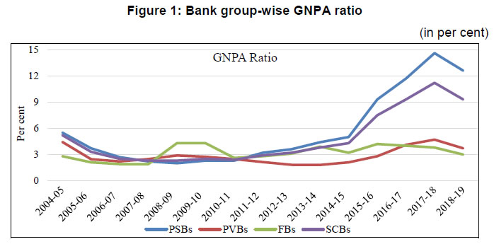 Besides, factors like adverse macroeconomic conditions, project delays, cost overruns, and absence of a strict bankruptcy code for faster resolution of stressed assets – also contributed to the deterioration in asset quality.7 Rising stress on the balance sheet of banks weighed on credit growth as it had a bearing on their profitability and capital position. The decline in credit growth reflects the fall in industrial production and earnings growth of the corporate sector and greater risk aversion of the banks.8 Thus, the demand-side and supply-side factors seem to have reinforced each other in the slowdown of credit growth (see Figure 1 and 2). 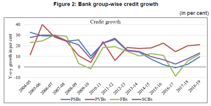 Considering the advances made by the banks to the non-financial firms, we find that the trend of non-performing loans as a percentage of total loans declined steadily from 11.4 per cent in 2001 to 2.2 per cent in 2009. However, this trend was reversed from 2010-11 onward. Non-performing assets with a high level of risk were initially hidden in the form of restructured standard advances. After the withdrawal of regulatory forbearance on asset classification of restructured accounts (April 2015), the asset quality review (AQR) of banks was undertaken by the Reserve Bank of India (RBI) in July-September 2015. It unearthed a large number of stressed assets in banks’ balance sheet and led the GNPA ratio of banks to jump from 4.3 per cent at end-March 2015 to 9.3 per cent at end-March 2017.9 The deterioration in banks’ balance sheet position can be assessed from its stability indicator of Z-score. The bank Z-score increased by 3.2 per cent during the pre-GFC period while it decreased by 8.9 per cent in the post-GFC era.10 2.3 Deterioration in macro-financial linkages We observe that the relationship between the macroeconomy and financial sector faces a logjam due to recurrent disturbances and adversities in the banking sector. Investment demand has become weaker with the twin balance sheet problem. The credit channel for feedback mechanism from the part of the monetary authority is not functioning well in an environment of high default risk of the borrower. Looking into the co-movements of the real and financial variables over the business cycles across the sub-periods of with and without financial stress, it is noticed that: (i) the procyclicality of investment to output has gone down, (ii) procyclicalities of the real price of the capital goods to investment and output have subdued,11 and (iii) the typical financial accelerator mechanism reflected in the countercyclical behaviour of credit and spread is disrupted (Table 2). | Table 2: Changing pattern of macro-financial linkages over business cycles | | Cross-correlations | 2002:Q2 - 2008:Q4 | 2009:Q1 - 2017:Q4 | | Output & Investment | 0.94*** | 0.77** | | Investment & Real Price of Capital Goods | 0.53*** | 0.03 | | Output & Real Price of Capital Goods | 0.47*** | -0.18 | | Bank Credit & Spread | -0.64*** | -0.04 | 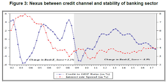 Further, we check the co-movements between credit-to-output ratio and interest rate spread across different phases of bank stability (Figure 3). During the period before 2009, the credit-to-output ratio moved countercyclically with the spread. The correlation coefficient between these two variables was -0.58 and statistically significant at one per cent level of significance. Such a countercyclical pattern has disappeared after 2009 indicating that macroeconomic and financial variables are not in sync to capture the presence of linkages between them. Mapping it with the developments in the banking sector, one can see that as the stability indicator (Z-score) declines the financial accelerator mechanism becomes less prominent. Notably, the banking sector stability has marked a significant decline when credit-to-GDP ratio has risen with a high level of risk premium. These empirical observations underscore the incidences of financial disturbances in the banking sector, which may have non-trivial effects on the inter-linkages between the financial system and the real economy. 3. Exploring micro-level evidence for identification of risk premium shock 3.1 Default risk, interest rate spread and growth rate of bank credit: connecting the dots A rise in the proportion of non-performing loans to total credit extended by the commercial banks indicates an increasing risk of default by the borrowers in their repayment behaviour. Based on the experience of global financial crisis, it is argued in the literature that the assessment of default risk is critically important to evaluate the risk premium on loans. Correct pricing of default risk influences the interest rate spread on credit and determines the pattern of credit growth. Addressing the pricing of default risk in the macroeconomy, Wickens (2017) mentions that credit spread can capture the risk of default adequately. Using a simple general equilibrium model with bank, he shows that a financial crisis would be very unlikely to occur if the probability of default is evaluated appropriately. If non-bank private sector and banks differ in this assessment, it would entail liquidity shortages and/or raise the external finance premium on loans. In other words, any unanticipated change in the default risk can be reflected through the changes in interest rate spread and/or the flow of credit. There is a consensus that the rise in default risk increases the risk premium on loans, hence interest rate spread, which reduces the supply of credit. To identify the financial shock emerging from the risk premium on credit, we first examine if interest rate spread increases with a rise in default rate; and second, if growth rate of real credit declines with a rise in the default rate. Our motivation is to provide empirical evidence from micro-level data to rationalize the sign restrictions used later to identify the risk premium shock at the macro-level in a structural VAR model. We measure the default risk using GNPA ratio. This indicator is used to evaluate the asset quality of banks and serves as a proxy for the probability of default of the borrowers. Any change in GNPA ratio implies a change in the risk premium. There are at least two distinct channels by which NPAs affect the bank lending activities. First, once a bank recognizes an account as NPA, provisioning requirements go up, which affects the balance sheet adversely and constrains the ability of the bank to make loans. Second, NPAs provide significant additional information about the state of the borrowing sector, which forces the bank to revise its expectations regarding future prospects of the assets, riskiness of the portfolio and pricing of the default risk for its new borrowers. While the first channel leads to significant decline in the supply of credit, the second one widens the gap between user cost and cost of funds for the bank. Using bank-wise panel data, we test the presence of these channels. Our approach, although differs purposively, has a resemblance with the literature discussing determinants of interest rate spread and growth rate of real credit. Rusuhuzwa, Karangwa and Nyalihama (2016) and Brock and Rojas-Suárez (2000) document the relationship between non-performing loans and spread. Besides, a stream of works exists suggesting that banks tighten the supply of credit if the condition of the borrowing sector worsens (Rajan, 1994; Weinberg, 1995; Asea and Blomberg, 1998; and Dell’Ariccia and Marquez, 2006). This argument is further reinforced by the empirical studies of Jimenez et al. (2012), Tomak (2013) and Cucinelli (2015), which show that credit risk has a negative impact on the lending behaviour of banks. In light of these studies, we examine how the default rate of borrower influences the risk premium on loan and the flow of bank credit, with due consideration to the possible endogeneity problems. 3.2 Data For our micro-level analysis, we use bank-level annual data for 2009-18. Though the share of non-bank financial companies has signficantly increased in recent years to fill the gap opened by the dwindling bank credit, their share in total loans remains low. At end-March 2009, the share of scheduled commercial banks (SCBs) and non-bank financial corporations (NBFCs) (adjusted for bank borrowings) in total loans and advances were 93.6 per cent and 6.4 per cent, respectively. By end-March 2018, the respective shares of SCBs and NBFCs (adjusted for bank borrowings) were 85 per cent and 15 per cent. Given the small share of NBFCs in total loans compared to SCBs, it appears to be more appropriate to focus on the latter for our study. The bank level data are sourced from the Statistical Tables Relating to Banks in India (STRBI) for the following variables: real credit growth, spread, GNPA ratio, capital to risk-weighted assets ratio (CRAR), deposit growth, deposit share, total assets, non-interest income, operating expenses, and Net Interest Margin (NIM).12 This data pertain to a panel of 55 Indian banks and include both private and public sector banks.13 Macroeconomic controls such as call money rate, real GDP, and capacity utilisation are taken from the Handbook of Statistics on Indian Economy and CMIE Economic Outlook, respectively. 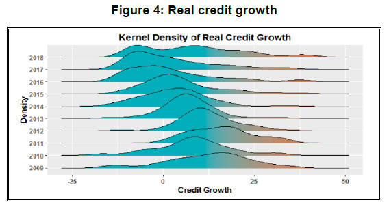 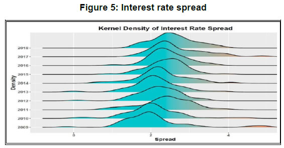 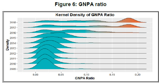 We control for a number of supply-side and demand-side factors which could possibly impact spread and credit growth in the empirical analysis. In the first panel estimation (spread on GNPA ratio), we control the relative size of a bank’s deposits by deposit share, the size of a bank by its total assets, financial conditions by its capital position (CRAR), the distribution of its earnings by the non-interest income ratio, operating efficiency by operating expenses to total assets, and macroeconomic effects by call money rate and capacity utilisation. In the second panel estimation (credit growth on GNPA ratio), deposit growth is included to capture the availability of loanable funds. NIM and CRAR are expected to control for the health of a given bank whereas logarithm of total assets accounts for the influence of size on credit growth. Real GDP and capacity utlisation are incorporated to encapsulate the demand-side factors. We choose these control variables primarily based on the existing empirical evidence while keeping in mind the specific characteristics of the Indian banking sector. A detailed description of all the variables are provided in Appendix 8.2 (see Table A.1). 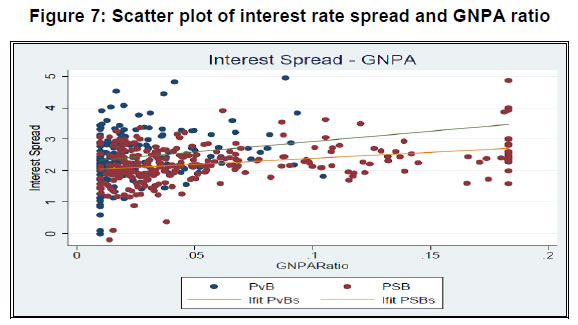 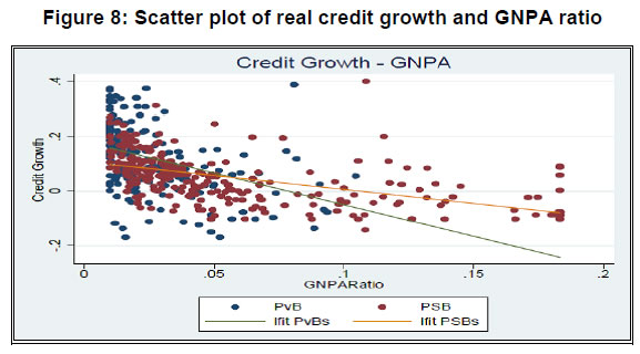 An eyeballing of the data on the variables of interest reveals interesting trends. Figure 4 indicates a shift in the distribution of real credit growth to the left over the years with the exception of 2011 and 2018, implying a decline in credit growth. Exactly the opposite seems to be happening with interest rate spread and GNPA ratio (see in Figure 5 and 6). The scatter plots (Figure 7 and 8) provide a reasonable depiction of the positive and negative relationship between GNPA ratio and spread, and GNPA ratio and real credit growth, respectively. Even though a discernible rightward shift in the distribution of spread is not much prominent (Figure 5), a positive association between the GNPA ratio and spread becomes apparent in the scatter plot (Figure 7). Absence of the rightward shift could possibly be due to other factors like the movements in interest rates that influence the spread. We control for those effects in the panel regression. 3.3 Methodology Going forward with the patterns observed in the graphs, we estimate the reduced form relationships between (i) spread and default rate; and (ii) credit growth and default rate using the bank-level panel data. The econometric models we estimate are as follows: 3.4 Estimation results In Tables 3 and 4, we report the results of dynamic panel estimation for interest rate spread and real credit growth regression on GNPA ratio. | Table 3: Interest rate spread and GNPA – Dynamic panel estimation models | | | (1) | (2) | (3) | (4) | (5) | | Spread | Spread | Spread | Spread | Spread | | L. Spread | 0.451*** | 0.353*** | 0.349*** | 0.308*** | 0.267 | | | (0.0855) | (0.108) | (0.111) | (0.0940) | (0.180) | | | | | | | | | GNPA Ratio | 0.0160* | 0.0310*** | 0.0315*** | 0.0407*** | 0.0547** | | | (0.00862) | (0.0110) | (0.0114) | (0.0125) | (0.0261) | | | | | | | | | L. Call money rate | 0.123** | 0.151*** | 0.150*** | 0.142*** | 0.230 | | | (0.0472) | (0.0478) | (0.0481) | (0.0473) | (0.159) | | | | | | | | | CRAR | | 0.0840** | 0.0840** | 0.112*** | 0.0936* | | | | (0.0342) | (0.0345) | (0.0367) | (0.0484) | | | | | | | | | Deposit share | | | -0.00702 | | -0.0109 | | | | | (0.00721) | | (0.0147) | | | | | | | | | Non-interest income ratio | | | | -0.0858 | | | | | | | (0.0994) | | | | | | | | | | Log of Total Assets | | | | -0.000419 | 0.000165 | | | | | | (0.000333) | (0.000752) | | | | | | | | | Operating expenses to Total Assets | | | | | 0.775 | | | | | | | (0.626) | | | | | | | | | Capacity Utilisation | | | | | 0.0873 | | | | | | | (0.0663) | | | | | | | | | Constant | 0.00386 | -0.00761 | -0.00727 | -0.00322 | -0.0839 | | | (0.00409) | (0.00526) | (0.00527) | (0.00645) | (0.0621) | | ar1 statistic | -3.38*** | -3.28*** | -3.25*** | -3.55*** | -2.90*** | | ar1p | 0.000726 | 0.00103 | 0.00114 | 0.000379 | 0.00372 | | ar2 statistic | -0.98 | -0.95 | -0.96 | -1.16 | -1.41 | | ar2p | 0.329 | 0.345 | 0.338 | 0.248 | 0.160 | | Sarganp | 0.362 | 0.673 | 0.687 | 0.936 | 0.152 | | Hansenp | 0.564 | 0.723 | 0.724 | 0.939 | 0.204 | | F | 16.58 | 21.48 | 17.55 | 21.85 | 8.128 | | Observations | 457 | 457 | 457 | 437 | 457 | Standard errors in parentheses
* p < 0.10, ** p < 0.05, *** p < 0.01 | From Table 3, it is noticeable that interest rate spread rises with the rise in GNPA ratio. The positive responsiveness is statistically significant across different specifications. This underscores the fact that as the default risk goes up, the risk premium on lending drives up the interest rate spread. In other words, when credit risk increases, commercial banks raise their interest rate spreads to hedge the risk of default. Our result is in line with Perez (2011) and Grenade (2007).15 Along with the default risk, we find that call money rate and CRAR influence the spread significantly. As argued in Gelos (2006) and Crowley (2007), a rise in interest rates could potentially reflect the increasing uncertainty in the economic enviornment, leading to an increase in spread. Besides, the relationship between capital adequacy and spread, although not straigntforward, it is observed that a better capitalised bank can (i) reap the benefit of lower funding costs (Ben Naceur and Goaied, 2008; Berger, 1995) and (ii) be in a position to invest in relatively riskier assets (Saunders and Schumacher, 2000). The positive and significant effect of CRAR on spread that we find in this paper is in line with the recent empirical evidence on Indian banks (John et al., 2016). Although other bank-specific controls such as deposit share, operating expenses, and non-interest income ratio have expected signs, they do not turn out to be statistically significant in this analysis.16 | Table 4: Real credit growth and GNPA – Dynamic panel estimation models | | | (1) | (2) | (3) | (4) | (5) | | Real credit growth | Real credit growth | Real credit growth | Real credit growth | Real credit growth | | L. Real credit growth | -0.200** | -0.0181 | -0.0144 | -0.0236 | -0.0298 | | | (0.0879) | (0.103) | (0.105) | (0.0965) | (0.0995) | | | | | | | | | Real deposit growth | 0.889*** | 0.852*** | 0.850*** | 0.869*** | 0.862*** | | | (0.0555) | (0.0525) | (0.0530) | (0.0531) | (0.0548) | | | | | | | | | GNPA Ratio | -0.603*** | -0.381*** | -0.315* | -0.356*** | -0.293* | | | (0.174) | (0.139) | (0.157) | (0.133) | (0.148) | | | | | | | | | CRAR | 0.797*** | 0.633*** | 0.511** | 0.481** | 0.491** | | | (0.271) | (0.223) | (0.229) | (0.220) | (0.211) | | | | | | | | | L.log of real GDP | 0.0161 | 0.0763** | 0.0644 | 0.0763** | 0.0632 | | | (0.0370) | (0.0364) | (0.0424) | (0.0335) | (0.0391) | | | | | | | | | Capacity Utilisation | | 0.751*** | 0.739*** | 0.764*** | 0.730*** | | | | (0.154) | (0.157) | (0.153) | (0.158) | | NIM | | | 0.893 | | 0.971 | | | | | (0.607) | | (0.621) | | | | | | | | | Log of Total Assets | | | | -0.00282 | -0.00245 | | | | | | (0.00292) | (0.00300) | | | | | | | | | Constant | -0.227 | -1.491*** | -1.358** | -1.443*** | -1.303** | | | (0.401) | (0.481) | (0.548) | (0.440) | (0.507) | | ar1 statistic | -3.58*** | -4.25*** | -4.21*** | -4.30*** | -4.26*** | | ar1p | 0.000342 | 0.0000215 | 0.0000250 | 0.0000174 | 0.0000203 | | ar2 statistic | -0.11 | 0.90 | 0.93 | 0.99 | 0.92 | | ar2p | 0.909 | 0.366 | 0.355 | 0.323 | 0.356 | | sarganp | 0.102 | 0.473 | 0.519 | 0.577 | 0.617 | | hansenp | 0.152 | 0.703 | 0.714 | 0.782 | 0.794 | | F | 102.5 | 157.2 | 126.6 | 166.3 | 148.3 | | Observations | 458 | 458 | 458 | 458 | 458 | | Standard errors in parentheses * p < 0.10, ** p < 0.05, *** p < 0.01 | Similarly, results in Table 4 establish a clear negative relationship between GNPA ratio and real credit growth. In line with the literature, these results indicate that a shock to the borrowing sectors, as captured by an increase in the GNPA ratio, will have a negative and significant impact on the credit growth, accentuating the credit crunch problem. While other bank-specific variables such as real deposit growth and CRAR significantly affect the growth in bank credit, demand side factors such as real GDP and capacity utilisation also exert a positive impact on the same, as expected. Real deposit growth signifies the expansion in the availability of loanable funds (Guo and Stepanyan, 2011) whereas a better capital position enables banks to handle adverse shocks effectively without denting their credit growth (Di Patti and Sette, 2012 and Jimenez et al., 2012).17 4. Understanding the effects of risk premium shock to banking sector using sign-restricted VAR (SRVAR) model 4.1 Choice of modelling framework For estimating the risk premium shock, it is imperative to use an appropriate identification procedure. Two methodological issues are involved in the identification of such shock. First, it is often difficult to disentangle the movements in supply of credit from the movements in demand for credit which complicates the extraction of shocks specific to the risk premium on credit. The reason is, on the one hand, the corporate sector may demand less credit due to cut down of their investments; on the other hand, financial intermediaries would also be reluctant to lend, and can either charge higher interest rates or decline more credit applications (Bernanke and Gertler, 1995; Oliner and Rudebusch, 1996). Second, it is also difficult to differentiate the exogenous movements in the supply of credit from the endogenous responses of the financial intermediaries with respect to changes in the macroeconomic and financial conditions. Given such empirical constraints in place, researchers have examined the economy-wide effects of the risk premium shock by exploiting the structural vector autoregression (SVAR) models. The SVAR framework offers a class of econometric models which is conditional on suitable identification scheme but remains relatively agnostic in nature to allow the data to determine the underlying structural dynamics. For our purpose, we choose a variant of the structural VAR, namely sign-restricted VAR (SRVAR) model, where restrictions are imposed on the signs of the impulse responses of the shocks of interest. The key advantages of a sign-identified structural VAR model are as follows. First, the number of shocks need not to be equal to the number of variables. Second, we do not need to impose any linear restrictions between the reduced form and structural form errors. It does not require the Cholesky type exclusion restrictions (i.e., point restrictions) on the impulse response coefficients, rather involves a more generic set-identification approach. Third, all the restrictions can be set directly on the shape of the impulse responses. These applied restrictions on the shape of IRFs are often invoked based on the impulse responses of relevant DSGE models, and therefore yield economically meaningful results. In view of these merits, researchers have used the SRVAR models to examine the shocks to financial sector. Majority of these works focus on the real effects (e.g., Hristov, Hulsewig and Wollmershäuser, 2012; Busch et al., 2010, Peersman 2012; Conti et al., 2015; Furlanetto et al., 2017; Gambetti and Musso 2017) and some of them examines the inflationary effect (Abbate et al., 2016; Meinen and Rheoe, 2018) of the shock. Following this body of literature, we implement an agnostic identification procedure to identify the risk premium shock to the Indian banking sector using SRVAR model. 4.2 Data We estimate the baseline SRVAR model with eight variables and present empirical impulse responses of the key macroeconomic and financial indicators for the risk premium shock. The sample period of the study is 2002:Q2 to 2017:Q4. Choice of sample period is driven by the availability of longest possible balanced sample for our analysis. All the data are taken from the Database on Indian Economy (DBIE). Our model includes real output (y), real consumption (cons), real investment (inv), consumer price inflation (infl), call money rate (cmr), real price of capital goods (rpqk), real bank credit (b) and interest rate spread (isp). We use seasonally adjusted consumer price index and compute the CPI inflation rate. Weighted call money rate is chosen as the closest indicator for the variations in policy repo rate. Interest rate spread is chosen as the proxy measure of risk premium on bank loans. Except for the rate variables, all other variables are log-transformed, seasonally adjusted and passed through Christiano-Fitzgerald (2003) asymmetric band pass filter in order to capture the effects over the business cycle frequency. Log-deviations of these variables from their trends are expressed in the percentage forms.18 In Figure 9, the pattern of time series is presented for all variables with the respective data transformation.19 4.3 Methodologies for estimation Different approaches are available in the literature for SRVAR modelling.20 We follow two methodologies from the literature: (i) the penalty function approach of Uhlig (2005) and (ii) the multiple shock identification approach of Arias et al. (2014). We produce the baseline models following both of these approaches and check the robustness of the results for alternative schemes of identification. Sign restrictions are imposed on the relevant variables with respect to the structural shocks, based on the micro-level evidence of bank-level panel data and the theoretical predictions of DSGE literature. While the penalty function approach of Uhlig (2005) offers partial identification of the structural shock, Arias et al. (2014) provides a more robust approach to isolate the shock of interest by discriminating it from the other possible structural and policy shocks.21 To ensure consistency, nevertheless, we compare the estimated shocks obtained from both methodologies and examine the coherence between them. 4.3.1 Identification of risk premium shock using penalty function approach Originally, Uhlig (2005) proposed the penalty function approach as an alternative to the pure sign restriction approach. Later, it has been modified with different types of loss functions to choose the impulse response vector of interest. The conventional rejection methods of Uhlig (2005) and Rubio-Ramirez et al. (2010) suggest that all impulse response vectors satisfying the imposed sign restrictions are considered to be equally likely. By construction, these methods will find only the impulse vectors that exactly satisfy the sign restrictions and discard others. For some cases, there could be only a few impulse response vectors satisfying the full set of restrictions. The penalty method, in contrast, assigns large numerical penalty to the models violating the sign restrictions. It not only penalizes for the violations of sign restrictions more than it rewards the models with correct signs, but also provides additional reward for large responses which can be tailored to specific responses and time-horizons. Hence, it offers a more efficient way to find out the impulse response vector that comes as close as possible to satisfy the imposed sign restriction. Following Uhlig (2005), Danne (2015) and Kilian and Lutkepohl (2017), we explain the econometric details of the model estimation below.22 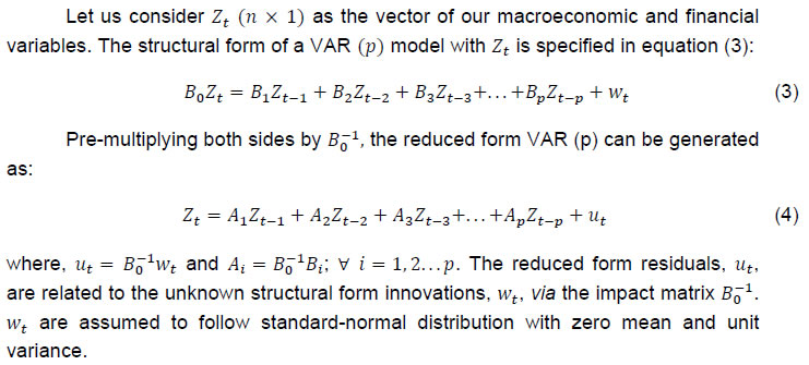
| Table 5: Sign restrictions for identification of risk premium shock | | | y | cons | inv | infl | cmr | rpqk | b | isp | | Case 1 | ? | ? | − | ? | ? | − | − | + | | Case 2 | ? | ? | ? | ? | ? | − | − | + | | Case 3 | ? | ? | ? | ? | ? | ? | − | + | At this stage, we neither have any information on the impact matrix nor we can observe the structural shocks, wt.23 In order to extract the information on impact matrix and identify the structural shocks, we impose restrictions on the sign of the impulse response vector of interest. In our context, this impulse response vector pertains to the shock that can affect the interest rate spread and real credit of the banking sector and transmit to investment and real price of capital goods. Following the theoretical predictions of Agenor and Zilberman (2015) and Agenor and da Silva (2017) regarding the effects of financial shock emerging from default risk, we impose sign restrictions on the relevant variables. At the same time, we remain agnostic about the effects of such a risk premium shock on the rest of the variables included in the model. Based on the results of our bank level panel estimation, we identify the risk premium shock emerging from high probability of default in terms of rise in interest spread and fall in the flow of credit. In consequence, private sector investment intermediated by bank credit is expected to drop and the real price of capital goods can contract through economy-wide general equilibrium effect. Accordingly, we impose positive sign restriction on spread and negative sign restrictions on credit, price of capital goods and investment. Given these sign restrictions in place, we start with a baseline model that is restrictive in nature, and then relax the sign restrictions one at a time to check the robustness for alternative identification schemes. 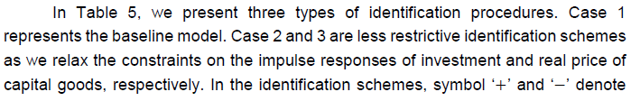  To check the significance of our model identification, we follow Fry and Pagan’s (2011) Median-Target (MT) method which works as a useful tool for diagnostic purposes. The goal of Fry and Pagan’s (2011) MT method is to find the single impulse vector that produces impulse responses which are as close to the median responses as possible. Strong differences between the MT impulse responses and the median responses indicate that the standard model inference is biased and misleading.25 We use the MT method to check the validity of the estimated SRVAR model. 4.3.2 Identification of risk premium shock with multiple structural shocks under Arias et al. (2014) approach The penalty function approach can identify only one shock at a time and is unable to accommodate multiple shocks in the identification procedure. This implies that the exogeniety of the shock to risk premium may be contaminated by the prevalence of other structural shocks. To ensure that the shocks of our interest truly capture their exogenous components and not any endogenous responses to the other disturbances, other potential structural shocks need to be included in the model with sign restrictions simultaneously (Paustian, 2007). Moreover, it is useful to set up an identification scheme combining the sign and zero restrictions on the impulse response functions to identify the relevant shocks uniquely. In such cases, while the sign restriction represents the action of constraining the response of a variable to a specific structural shock to be positive or negative, zero restrictions represent the action of constraining the response of a variable to a specific structural/policy shock to take the value of zero. We use the approach of Arias et al. (2014) to identify and estimate the risk premium shock, along with the identification of other structural shocks. This algorithm provides a more efficient and statistically robust method of estimation compared to other alternatives.26 While the Cholesky or triangular factorization schemes allow generating constraints over the contemporaneous responses only (i.e., period of impact in the impulse response functions), the general restriction methodology proposed by Arias et al. (2014) permits to implement restrictions at any period of the impulse responses. Following Dieppe et al. (2018), we have explained the estimation process and provided the description of algorithm in Appendix 8.4. Rationale behind identification schemes: Under the Arias et al. (2014) approach, we set up the identification scheme for the baseline specification using zero and sign restrictions as laid out in Table 6. Such an identification scheme is motivated by the theoretical predictions of DSGE models.27 In our eight-variable SRVAR model, we allow eight different types of shocks which can drive the business cycle fluctuations in an EME like India. This includes shocks to fiscal spending (FP), consumption demand (AD), marginal efficiency of investment (MEI), aggregate supply (AS), monetary policy (MP), capital quality (KQ), demand for credit (CD) and risk premium (RP). We consider all the shocks of contractionary types. We impose the sign restrictions on impact and allow it to vary up to four quarters. Note that in this identification scheme, cells containing zero denote the zero restriction on the corresponding shock. | Table 6: Identification of risk premium shock under Arias et al. Approach (2014) - Scheme 1 | | | FP | AD | MEI | AS | MP | KQ | CD | RP | | y | − | ? | ? | − | 0 | ? | ? | ? | | cons | ? | − | + | ? | ? | ? | ? | ? | | inv | ? | ? | − | ? | ? | ? | ? | − | | infl | − | − | − | + | 0 | 0 | ? | ? | | cmr | − | ? | ? | ? | + | 0 | ? | ? | | rpqk | ? | ? | ? | ? | ? | − | ? | − | | b | ? | ? | ? | ? | − | ? | − | − | | isp | ? | ? | ? | ? | + | + | − | + | A spending cut from the fiscal side leads to the fall of output, inflation and policy rate (Gabriel et al., 2012). So, negative sign restrictions are taken for these variables. Shock to aggregate demand is assumed to surface from consumption via shift in preference (Ireland, 2004). Due to an adverse change in preference if the private consumption declines, it can lead to a decline in inflation. To identify a negative aggregate demand shock, we restrict consumption and inflation to decline. These restrictions are in line with the DSGE model predictions (Erceg et al., 2000; Smets and Wouters, 2003). Shock to marginal efficiency of investment is incorporated as it can be one of the major sources of fluctuations in investment (Justiniano et al., 2010). MEI shock affects the production of installed capital from investment goods and influences the transformation of savings into future capital input. It is evident from the literature that a negative MEI shock contracts investment, raises consumption and pacifies inflation. For the supply side or cost push shocks, output and prices move in the opposite directions (Fry and Pagan, 2011). Thus, we ascribe output to decline and inflation to rise for an adverse aggregate supply shock. In case of a shock to credit demand, a negative surprise, sourced from either a sudden change in the valuation of collateral or restrictive macroprudential policy, induces the interest rate spread to go down (Brzoza-Brzezina and Makarski, 2011). So, the impulse responses of the volume of bank credit and interest rate spread are expected to be unidirectional. For the identification of the monetary policy and capital quality shocks, we use the combination of zero and sign restrictions. The reasons are as follows. First, Paustian (2007) and Fry and Pagan (2011) argue that the structural shocks are appropriately identified with sign restrictions only if they have a major impact on the system. While the aggregate demand or supply side shocks explain the economic fluctuations to a greater extent, monetary policy shock accounts for a small fraction of the same, especially in the EMEs. It is also difficult to filter out from the risk premium shock on credit as both can drive the credit and spread in the similar directions. Additionally, it is well known that output and inflation hardly respond contemporaneously for a policy rate shock (Christiano et al., 1999).28 Hence, we impose appropriate sign restrictions on the policy rate, spread and credit with zero restrictions on output and inflation. Second, the capital quality shock may behave like a risk premium shock as both of them can impact the price of capital goods and spread in the same fashion (Sanjani, 2014). However, the transmission of capital quality shock to consumer price inflation and the subsequent response of the monetary authority via policy rate may not be contemporaneous in nature. Hence, we impose zero restrictions on inflation and policy interest rate contemporaneously and isolate it from the risk premium shock. Finally, for the risk premium shock, we retain the same sign restrictions on interest rate spread, credit, real price of the capital goods and investment as used in the penalty function approach. As interest rate spread is expected to react immediately, even before the volume of credit, due to change in the level of riskiness associated with lending, spread is ordered at the end after the credit variable. This pattern of ordering distinguishes the risk premium shock from the shock to credit supply. Robustness check with alternative identification schemes: | Table 7: Alternative identification under Arias et al. Approach (2014) - Scheme 2 | | | FP | AD | MEI | AS | MP | KQ | CD | RP | | y | − | ? | ? | − | ? | ? | ? | ? | | cons | ? | − | ? | ? | ? | ? | ? | ? | | inv | ? | ? | − | ? | ? | ? | − | − | | infl | − | − | − | + | ? | ? | ? | ? | | cmr | ? | ? | ? | ? | + | ? | ? | ? | | rpqk | ? | ? | ? | ? | ? | − | ? | − | | b | ? | ? | ? | ? | ? | ? | − | − | | isp | ? | ? | ? | ? | + | + | − | + |
| Table 8: Alternative identification under Arias et al. Approach (2014) - Scheme 3 | | | FP | AD | MEI | AS | MP | KQ | CD | RP | | y | − | ? | ? | − | ? | ? | ? | ? | | cons | ? | − | ? | ? | ? | ? | ? | ? | | inv | ? | ? | − | ? | ? | ? | ? | ? | | infl | − | − | − | + | ? | ? | ? | ? | | cmr | ? | ? | ? | ? | + | ? | ? | ? | | rpqk | ? | ? | ? | ? | ? | − | ? | ? | | b | ? | ? | ? | ? | ? | ? | − | − | | isp | ? | ? | ? | ? | + | + | − | + | To check the robustness of the effects of risk premium shock in presence of multiple structural shocks, we explore alternative identification schemes with pure sign restrictions. The reason we depart from zero restrictions is to examine if the key results hold in a less restrictive environment. In Tables 7 and 8, alternative schemes of identification are presented. In Identification Scheme 2, we remove zero restrictions on the monetary policy shock and capital quality shock but remain restrictive on the responsiveness of investment to credit demand and risk premium shocks. In Identification Scheme 3, we drop those restrictions and take an agnostic position on the reaction of investment to both credit demand and risk premium shock to allow the data to speak more for the underlying transmission mechanism. 4.4 Empirical findings 4.4.1 Results obtained from penalty function approach Impulse response analysis: 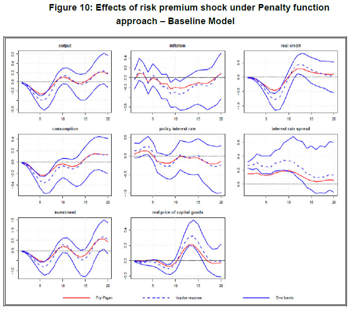 The impulse response plots of Figure 10 depict an economy-wide contractionary effect of a positive risk premium shock. Given the sign restrictions imposed by Identification Scheme 1, one standard error shock to risk premium raises interest rate spread by 0.3 per cent and decreases the real credit by 0.75 per cent approximately. Real price of capital goods becomes depressed for a prolonged period and reverts to its long run level after ten quarters. Although the fall in real credit is quite pronounced, the downturn in the real price of capital goods does not appear to be that sharp (-0.1 per cent). In contrast, real variables like output, consumption and investment show a significant contraction in their dynamic responses. The peak effect of contraction takes place around fifth to sixth quarter after the shock and reduces private consumption by 0.35 per cent, investment by 0.8 per cent and aggregate output by 0.4 per cent. Inflation shows a spurt at the impact period. But, it goes down from third quarter onwards and remains low over fifteen quarters until it reverts to the long-run level. The call money rate follows a trajectory similar to that of inflation and shows a negative response after the initial periods of rise. This indicates that policy interest rate moves in line with the movements of CPI inflation rate. On the whole, it is found that the contractionary effects of a positive risk premium shock persist on nominal and financial variables much longer than on real variables. Further, it is observed that the median impulse response of the variables under Uhlig’s penalty function approach closely resembles with the one prescribed by Fry and Pagan (2011) median targeting strategy. After first few quarters of deviation, median impulse response suggested by Fry and Pagan (2011) comes within the confidence band of IRF plots. This provides a diagnostic check for the reliability of observed IRFs of the risk premium shock under the penalty function exercise. Robustness checking of IRF properties under alternative schemes of identification: The IRF plots and subsequent results described so far are obtained from the identification strategy of Case 1 which is considered as the baseline model. However, this identification scheme is restrictive as it imposes sign restrictions on the intermediate variables of transmission process like real price of capital goods and investment. To check the robustness of the IRFs, therefore, we examine the identification strategies of Case 2 and Case 3. Relaxing the number of sign restrictions, we re-run the baseline SRVAR model with penalty function approach and observe similar patterns in the IRFs. These plots are presented in Figure A.4 and A.5 in Appendix 8.5. Baseline results of FEVD: Results of forecast error variance decomposition (FEVD), which is conditional over different time horizons such as one quarter ahead, ten quarters ahead and twenty quarters ahead, reveals the strength of risk premium shock over the business cycle. Table 9 presents the contribution of risk premium shock (in per cent) to the fluctuations of all variables at different time horizons of forecast. | Table 9: FEVD results from baseline model under Penalty function approach | | Quarter | y | cons | inv | infl | cmr | rpqk | b | isp | | 1 | 25.7 | 22.3 | 12.9 | 4.4 | 5.1 | 18.1 | 11.2 | 24.4 | | 10 | 20.9 | 20.6 | 18.9 | 12.9 | 12.6 | 16.4 | 21.8 | 23.3 | | 20 | 20.6 | 20.3 | 19.8 | 14.2 | 14.4 | 20.4 | 21.3 | 20.6 | Effect of risk premium shock varies over the time horizon and across the variables. Our observations are as follows. First, output effect of the shock is substantial. It explains around one-quarter of the variations in GDP for the shorter time horizon of forecast. Although the impact declines gradually over time, it can still account for 20 per cent of the output fluctuations in the economy. Considering the key constituents of aggregate demand, such as consumption and investment, we find some difference in the role of risk premium shock. Private consumption is considerably affected by the financial disturbance. Approximately 20 per cent of the variations in private consumption are explained over the short to medium-term time horizon. In case of investment, the shock explains the variations slightly lesser in magnitude. However, as we extend the time horizon of forecasting from one-quarter to twenty quarter ahead, the impact of shock magnifies from 13 per cent to 20 per cent. It is noticeable that the impact of the shock on consumption declines over time but accentuates for the investment. The FEVD pattern of investment is also reflected from the bank credit. We observe that the contribution of the shock is amplified as we move from the short to long horizon of forecast. This increasing effect of the shock is also apparent from the movements of inflation rate and policy interest rate. Typically, the prominence of risk premium shock on inflation shows up nearly after ten quarters with a rise from 4.4 per cent to 14.2 per cent. In contrast, contribution of the shock to asset price fluctuation remains moderately steady around 18 per cent over the forecast horizons. 4.4.2 Results obtained under multiple structural shock identification approach Impulse response analysis: Under the multiple structural shock identification approach of Arias et al. (2014), the pattern of IRFs of risk premium shock is found qualitatively similar to the ones that are observed under the penalty function method. However, the quantitative differences do exist between these two approaches. The effects of the shock appear to be less pronounced under the multiple shock identification approach compared to the penalty function approach. In Figure 11, impulse responses are plotted. The key features of the IRFs are as follows. First, real output and its constituents like private consumption and investment – all decline together with impact of the shock by 0.01 per cent, 0.005 per cent and 0.011 per cent, respectively. This contraction on real variables continues nearly for twelve quarters. Second, among the constituents of output, it is observed that the fall in investment is significantly more than that of consumption. Considering the accumulated effect of the shock over the span of twelve quarters, it is noticed that investment drops by 0.32 per cent while consumption reduces by 0.22 per cent. Nevertheless, investment reverts to its long run equilibrium level slightly faster than consumption. Such behavioural patterns of consumption and investment is in line with the findings of Duchi and Elbourne (2016). Third, it is evident that a positive shock to risk premium is deflationary in nature. The accumulated effect over the period of twelve quarters shows 0.36 per cent decline in CPI inflation. This deflationary effect of an adverse financial shock has a strong resemblance with the theoretical predictions of Curdia and Woodford (2010), Ajello (2016), and Agenor and Zilberman (2015) and is in conformity with the empirical findings of Gambetti and Mussa (2017) and Furlanetto et al. (2017). Fourth, policy rate follows the path of inflation with a lag which highlights the inflation stabilizing role of the monetary authority. Fifth, real price of capital goods decreases and attains the peak effect after six quarters with a 0.042 per cent decline from its long run level. Finally, a shock to risk premium can raise the interest rate spread by more than one percent over the medium term and depress the bank credit by 0.57 per cent. Overall, the contractionary effect of an adverse shock to the risk premium on bank credit becomes visible from all segments of the economy. 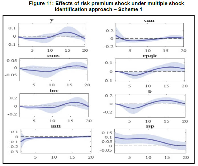 Following the properties of impulse responses, one can trace out the process of transmission and propagation of the shock. A shock to risk premium amplifies the spread and thereby tightens up the friction in the credit market. This entails to a reduction in the flow of credit via bank lending channel. The asset price channel also operates parallel to the bank lending channel. Due to the anticipation of high default risk of the prospective investment projects, demand for the capital goods shrinks which may cause a depreciation in the real prices of capital through the asset price channel. With the crash in the capital goods price, return from capital accumulation decreases and subsequently, demand for investment plunges. Slack in the availability of credit further reinforces the contraction in investment. Private consumption also goes through a slump as the opportunity cost of current consumption rises. This takes place as an inter-temporal reaction of the economic agents to higher interest rate spread and operates through the interest rate channel. Fall in the demand for consumption and investment drives down the aggregate output. In sum, an adverse shock to the risk premium on bank credit sets in economy-wide contractionary effects through a multi-pronged transmission mechanism.29 Robustness checking of IRF properties under Arias et al. (2014) approach for alternative schemes of identification: As mentioned in the description of methodology, we check the robustness of impulse response properties of SRVAR model with respect to alternative identification strategies. We change the identification scheme of baseline model, i.e., Identification Scheme 1, incrementally and move towards a more generic pure sign restriction to examine the reliability and consistency of the IRFs.30 Under Arias et al. (2014) approach, the IRFs are obtained from Identification Scheme 2 and 3 and presented in Figure A.6 and A.7 in Appendix. The patterns of the IRFs appear to be qualitatively similar. Nevertheless, the quantitative difference in the impulse responses becomes apparent across the identification schemes. To check this further, we extract the median IRF of each variable with respect to risk premium shock and plot them together to analyze their responsiveness for alternative identification strategies. This plot is provided in Figure 12 (A and B). Additionally, we have documented the magnitude of peak effect (in per cent) of the shock on each variable and the corresponding period of occurrence in Table 10.31 Examining the peak effects of the risk premium shock, we find that a relaxation in the restrictions trims down the magnitude of effect of the shock. It moderates the effect on nominal and financial variables in particular, and does the same for real variables but to a lesser extent. Besides, it also alters the period of occurrence of peak effect of contraction. So, one can infer that a less restrictive model can provide us at least a conservative estimate regarding the effect of the shock, whereas a more restrictive model would be needed to measure the intensity of the same.32 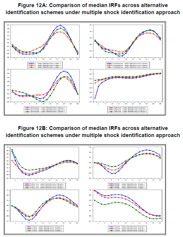
| Table 10: Comparing peak effect of contraction for different identification schemes | | Identification Schemes | y | cons | inv | infl | | Size | Qtr. | Size | Qtr. | Size | Qtr. | Size | Qtr. | | Scheme 1 | -0.031 | 5 | -0.028 | 8 | -0.044 | 9 | -0.102 | 1 | | Scheme 2 | -0.028 | 4 | -0.022 | 8 | -0.035 | 4 | -0.039 | 1 | | Scheme 3 | -0.028 | 8 | -0.025 | 8 | -0.059 | 10 | -0.027 | 1 | | Identification Schemes | cmr | rpqk | b | isp | | Size | Qtr. | Size | Qtr. | Size | Qtr. | Size | Qtr. | | Scheme 1 | -0.062 | 6 | -0.042 | 6 | -0.113 | 6 | 0.098 | 1 | | Scheme 2 | -0.055 | 6 | -0.029 | 6 | -0.083 | 6 | 0.096 | 1 | | Scheme 3 | -0.033 | 6 | -0.016 | 6 | -0.087 | 6 | 0.059 | 1 | Results of FEVD from baseline model: The FEVD results of risk premium shock under Arias et al. (2014) approach is broadly in line with the results obtained under penalty function approach with some quantitative differences. The results for one quarter, ten quarter and twenty quarter ahead time horizon are presented in Table 11 (in per cent). In addition, a comprehensive plot with respect to each period (up to twenty quarters) is provided in Figure A.8 in Appendix 8.8. It is evident that, except inflation, policy interest rate and real price of capital goods, the prominence of the financial shock in driving the fluctuations dissipates gradually as the time horizon of forecast increases. However, the output effect of financial shock seems to be substantial at a shorter horizon of forecast if we compare it with the penalty function approach. | Table 11: FEVD results from baseline model under multiple shock identification approach | | Quarter | y | cons | inv | infl | cmr | rpqk | b | isp | | 1 | 31.2 | 14.2 | 17.4 | 7.9 | 4.9 | 5.1 | 22.7 | 35.1 | | 10 | 11.8 | 10.6 | 7.6 | 10.5 | 11.5 | 17.6 | 17.2 | 33.9 | | 20 | 12.1 | 10.3 | 9.9 | 11.2 | 11.4 | 20.9 | 18.6 | 29.1 | Historical decomposition of shocks: Along with forecast error variance decomposition, we investigate the historical decomposition of the variables with respect to structural shocks included in the baseline SRVAR model and present it in Figure 13. It is evident that the role of financial disturbance in the form of risk premium shock becomes quite significant in the post-2009 period in driving the macroeconomic and financial variables. More specifically, during the year of 2015 and its adjacent quarters, risk premium shock makes a striking impact in the downturn of consumption, investment and aggregate output. This empirical finding is in concurrence with the micro-level evidence obtained from the bank-wise panel estimation. The results of panel estimation suggests that the rate of loan default is one of the determinants of the rising interest rate spread and declining credit growth in the post-2009 period. Reinforcing this observation and extending it further, the macro-level analysis underscores that the financial disturbance, which emanates in the form of a risk premium shock, could be one of the major sources of economic fluctuations in India during the post crisis period. 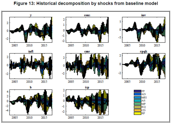 4.5 Robustness checking of shock identification between penalty function and multiple shock approaches In our analysis, we have examined the robustness of results obtained from two methodologies of SRVAR model estimation. We have discussed the robustness of results for different identification strategies under the penalty function approach of Uhlig (2005) and multiple shock identification of Arias et al. (2014) individually. However, one can be curious to explore if these methodologies are capable to produce a comparable series of the shocks of interest. In other words, is the risk premium shock identified under Uhlig’s approach similar to the one identified under Arias et al. (2014) method? This question is important to examine on two accounts. First, it can ensure that the identified series of financial shock is robust to the choice of methodology. Second, in a broader context, this exercise can enable us to understand the discrepancies between partial identification and multiple structural shock identification approaches. We extract the representative series of risk premium shock obtained under partial identification and multiple shock identification approaches across the alternative identification schemes and plot them in Figure 14. Comparing both the series of risk premium shock, we find the following observations. First, both the series are statistically significantly correlated at five per cent level of significance with correlation coefficient 0.26. This suggests that the risk premium shock is well identified in our analysis and robust to alternative methodologies of SRVAR estimation. Second, as we check the coherence between both series for pre-2009 and post-2009 period, it appears that correlation coefficient (0.47) is highly significant during pre-2009 but goes down drastically (0.07) during the period of post-2009 period. This indicates that partial identification and multiple shock identification can produce a converging result during the tranquil phase of the sample period. During the period of turmoil, as the size of underlying structural shocks rises, the results of shock identification may differ substantially. 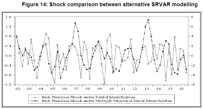 5. Examining the alternative forms of financial shocks and efficacy of policy interventions In our analysis so far, we have identified a positive shock to risk premium on bank credit and quantified its contractionary effects through different macroeconomic and financial variables. In addition to these results, we explore two relevant issues further. We extend our empirical exercise to examine (i) the quantitative significance of alternative forms of financial shocks in the banking sector in comparison to the risk premium shock; and (ii) the role of alternative policy interventions to curb the contractionary output effect of the risk premium shock. To perform these two objectively different but structurally related experiments, we exploit the SRVAR framework with a six variable configuration and estimate the model with multiple structural shock identification approach. Methodologically, we depart from the eight variable baseline SRVAR model of Section 4 for the following reasons. First, both the experiments are designed to provide the quantitative assessment rather than disaggregated illustration of shock transmission mechanism. Hence, the reduction of dimension is done to improve the computational efficiency. Second, since this empirical analysis involves a horse racing among the alternative forms of financial shocks and mode of policy interventions, we use a pure sign restriction based identification for all the shocks and impose restrictions only on the source and outcome variables.  5.1 Assessing the relative strength of alternative financial shocks to banking sector The identification scheme of three different types of financial shocks are proposed in Table 12. For the shock to banking sector stability, we impose negative sign restriction on bank z-score, positive sign restriction on interest rate spread and a negative response on output (Gerali et al., 2010). Similar type of output contractionary adverse shocks are considered for credit demand and risk premium. The key difference between them is that for a positive risk premium shock, spread rises and credit falls; but for a negative credit demand shock, credit and spread both falls together. | Table 12: Baseline for policy simulation - Identification scheme | | | AD | AS | MP | BK | CD | RP | | y | − | − | ? | − | − | − | | infl | − | + | ? | ? | ? | ? | | cmr | ? | ? | + | ? | ? | ? | | z − score | ? | ? | ? | − | ? | ? | | b | ? | ? | ? | ? | − | − | | isp | ? | ? | + | + | − | + | From the historical decomposition, we trace out the contribution of the financial shocks to fluctuations of macroeconomic variables. Figure 15 reveals that each type of financial shock, by and large, has contributed to the economic fluctuations throughout the sample period. Typically, during 2008-09 and its subsequent period, their predominance has increased specially for the credit and output. Narrowing down our focus on the relative strength of each type of financial shock, we look into the impact effect, twelve-quarter accumulated effect, and forecast error variance decomposition of output and inflation. From Table 13, we find that risk premium shock is at least as prominent as the credit demand shock. In particular, it supersedes the credit demand shock marginally at the impact effect on output and bank stability shock on the accumulated effect. For inflation, shocks have differential effects when compared based on the impact and accumulated effects. However, the risk premium shock consistently shows a stronger deflationary effect.
| Table 13: Comparing effects of alternative financial shocks (in per cent) | | | Output | Inflation | | | Effects | BK | CD | RP | BK | CD | RP | | Impact Effect | -0.008 | -0.015 | -0.015 | 0.268 | -0.005 | -0.044 | | Accumulated Effect | -0.11 | -0.079 | -0.113 | 0.259 | 0.066 | -0.201 |
| Table 14: Comparing FEVD results of alternative financial shocks (in per cent) | | Period | Output | Inflation | | BK | CD | RP | BK | CD | RP | | 1 | 2.80 | 9.07 | 8.64 | 14.29 | 5.52 | 7.37 | | 10 | 9.26 | 5.27 | 7.19 | 13.81 | 5.72 | 7.73 | | 20 | 8.93 | 5.42 | 7.49 | 13.82 | 5.72 | 7.94 | Considering the FEVD results at different horizons from Table 14, we observe that the contribution of risk premium shock across different time horizons, magnitude-wise, lies between the share of bank stability and credit demand shocks in driving the output fluctuations. This result underlines the fact that a shock to bank stability matters more in the medium run while a shock to credit demand drives the short run variations in output. In comparison, risk premium shock makes its presence visible at all time horizons of the forecast. In case of inflation, it is found that bank stability shock dominates over the other types of financial shocks. One possible explanation here is that, the cost-channel transmission via working capital requirement of firms may become stronger. If the commercial banks are well-capitalized and in stable condition, the transmission of a positive or negative shock to the borrowing firms would be lesser subject to their borrowing requirements for working capital. In other words, cost of production would be less sensitive to lending rates if the financial intermediary is in a position to absorb the exogenous shock. This supply-side implication may have magnified the role of shocks to bank stability in driving inflation. 5.2 Results from policy simulation In view of the adverse effects of risk premium shock in an EME like India, we investigate alternative modes of policy interventions that can minimize the contraction of economic activities. The motivation has come from the long standing debate on the relative efficacy of the two macroeconomic stabilization policies, i.e., monetary policy vis-a-vis fiscal policy, in stimulating growth and ensuring price stability. Pereira (2012) provides evidence of temporal variation in the effectiveness of monetary and fiscal policies in case of the US on the basis of a SVAR model with joint identification of the respective shocks. Using VAR model, Hussain (2014) shows that monetary policy has been more effective than fiscal policy in case of Pakistan and Sri Lanka, whereas fiscal policy has a more powerful effect than monetary policy in Bangladesh, India and Nepal. Richard et al. (2018) argue that monetary policy is more effective than fiscal policy in explaining the changes in output, while Özer and Karagöl (2018) found that it is other way round. As it stands now, the relative merit of these policies depends upon the structure of economy, institutional arrangements of the markets and stage of development. 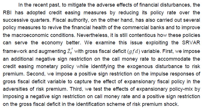 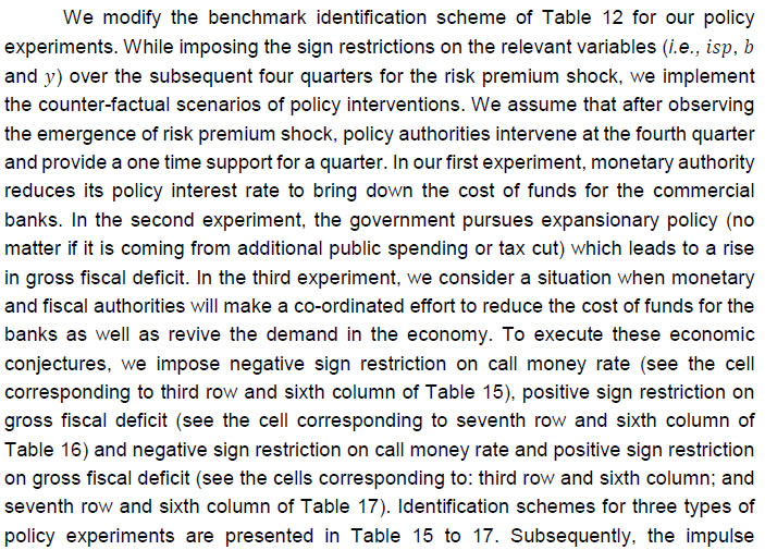 
| Table 15: Recovery by credit easing policy - Identification scheme | | | AD | AS | MP | BK | CD | RP | FS | | y | − | − | ? | − | − | − | − | | infl | − | + | ? | ? | ? | ? | − | | cmr | ? | ? | + | ? | ? | − | ? | | z − score | ? | ? | ? | − | ? | ? | ? | | b | ? | ? | ? | ? | − | − | ? | | isp | ? | ? | + | + | − | + | ? | | gfd | ? | ? | ? | ? | ? | ? | − |
| Table 16: Recovery by expansionary fiscal policy - Identification scheme | | | AD | AS | MP | BK | CD | RP | FS | | y | − | − | ? | − | − | − | − | | infl | − | + | ? | ? | ? | ? | − | | cmr | ? | ? | + | ? | ? | ? | ? | | z_score | ? | ? | ? | − | ? | ? | ? | | b | ? | ? | ? | ? | − | − | ? | | isp | ? | ? | + | + | − | + | ? | | gfd | ? | ? | ? | ? | ? | + | − |
| Table 17: Recovery by expansionary policy-mix - Identification scheme | | | AD | AS | MP | BK | CD | RP | FS | | y | − | − | ? | − | − | − | − | | infl | − | + | ? | ? | ? | ? | − | | cmr | ? | ? | + | ? | ? | − | ? | | z_score | ? | ? | ? | − | ? | ? | ? | | b | ? | ? | ? | ? | − | − | ? | | isp | ? | ? | + | + | − | + | ? | | gfd | ? | ? | ? | ? | ? | + | − | From the plots of Figure 16 (A and B), it is evident that output contraction for a risk premium shock can be lesser if any type of expansionary policy intervention takes place. The response of inflation also pacifies more compared to our baseline estimates, except in the case of credit easing policy. The pronounced drop in the output can be arrested when the banking sector is suppoerted by the credit easing monetary policy. Reduction in the policy rate lessens the cost of funds in the inter-bank market which can help the banks to absorb the default risk of loans partially and charge a relatively lower interest rate on their lending that can generate a favourable effect via credit channel. In case of expansionary fiscal policy intervention, the overall demand condition improves and drives up the return from the investment projects and investment in the economy. With the increasing real rate of return from the investment projects, repayment of loans will improve and provide banks some respite.33 In case of the expansionary policy mix, we observe quantitatively better response of output and inflation to risk premium shock. This incremental gain comes from the fact that the potential crowding out effect of the fiscal expansion is offset by the credit easing policy of the monetary authority. Hence, the positive demand effect on output strengthens and inflation is moderated to a greater extent through cost-channel. 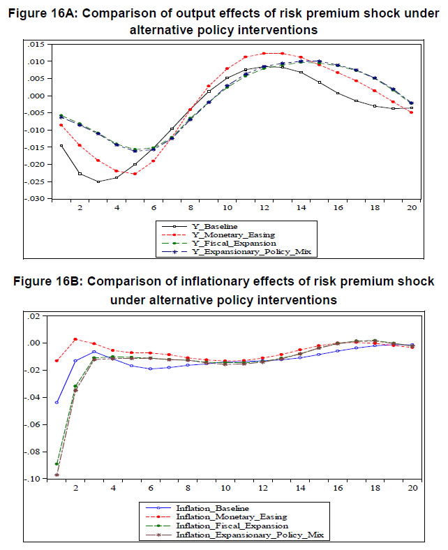
| Table 18: Comparing effects of risk premium shock under alternative policy responses | | (in per cent) | | Output | | Different types of Effects | Benchmark Model | Monetary Easing | Fiscal Expansion | Monetary Easing & Fiscal Expansion Mix | | Impact Effect | -0.015 | -0.009 | -0.006 | -0.006 | | Peak Effect | -0.025 | -0.023 | -0.016 | -0.016 | | Accumulated Effect | -0.113 | -0.088 | -0.075 | -0.076 | | Inflation | | Impact Effect | -0.044 | -0.013 | -0.089 | -0.097 | | Peak Effect | -0.044 | -0.013 | -0.089 | -0.097 | | Accumulated Effect | -0.202 | -0.100 | -0.246 | -0.263 | To evaluate the quantitative significance of alternative policy interventions, we check out the impact effect, peak effect and accumulated effect (over twelve quarters) of the risk premium shock on output and inflation with respect to the benchmark model, and document the same in Table 18. Magnitudes of the effects suggest that any kind of expansionary policy intervention reduces the contraction in output. Individually, the support from monetary policy helps to subdue the contraction of output but comes at the cost of higher inflationary outcome. Fiscal expansion, on the other hand, does well in trimming down the predominance of risk premium shock in output while curbing the inflation to a greater extent compared to the monetary policy. Nevertheless, the expansionary policy-mix seems to perform moderately better in contrast to the individual expansionary policy interventions. It reduces the degree of output contraction and ensures a low inflation environment compared to other policy options across different measurements of the effects. This result, on the whole, suggests that to revitalize the business cycle that is impacted by the disturbance in risk premium, monetary and fiscal policy instruments should work in tandem. 6. Conclusion In the backdrop of deceleration in credit growth in the post-GFC period with the balance sheet repairs in banks being at varying stages in major EMEs, Indian banks witnessed slowdown in the flow of bank credit coupled with rising NPAs starting from 2012. This exacerbated the downturn in business cycle as the twin balance sheet problem and high degree of risk aversion hit both banks and non-financial corporates. This was accompanied by weakening capital position and declining profitability of banks, and raised the question as to whether high asset impairments and resultant high risk premium led to the slowdown in credit growth. We have addressed this question using both micro and macro-level analysis in this study. Besides, we explore alternative policy interventions to mitigate the adverse effects of a risk premium shock on the economy. In the micro-level analysis, it is found that the interest rate spread, attributed to risk premium on loans, increased in response to a rise in loan defaults during the post-2009 period. Also, credit growth is found to be negatively associated with the loan default rate, indicating that a shock to the borrowing sectors has a significant negative impact on credit growth. Premised on the micro-level observation, the macro-level analysis suggests that a financial disturbance like a risk premium shock could be one of the major sources of credit and business cycle fluctuations in India. More specifically, SRVAR results under the penalty function approach suggest that a positive shock to risk premium leads to an uptick in interest rate spread and a decline in bank credit and real price of capital goods. The contractionary impact is also visible from the real sector variables such as output, consumption and investment. However, such adverse effects of a positive risk premium shock persist on the financial variables for much longer period of time as compared to the real variables. Under the multiple shock identification approach, though we observe similar results, the impact of the shock becomes less pronounced. Our findings on the business cycle effects of an adverse risk premium shock are quantitatively similar to that reported for advanced economies (Meeks, 2012; Duchi and Elbourne, 2016; Hristov et al., 2012) as well as for EMEs (Benes et al., 2009; Cambazoğlu and Karaalp, 2013), but in contrast to the study of Xue and Zhang (2019). According to Xue and Zhang (2019), the impact of credit shocks on business cycles is much larger in case of the EMEs compared to the advanced economies due to their high dependence on bank credit. To minimize the contractionary output effects of a risk premium shock, we also investigated the relative effectiveness of alternative modes of policy interventions. Our policy experiments reveal that an expansionary policy mix of fiscal and monetary policies may perform better than the individual-level intervention of expansionary monetary or fiscal policy to mitigate the economic downturn as the demand side channel can be complemented with a conducive monetary transmission mechanism from the supply side. Given the fact that our analysis relies on alternative SRVAR models, a caveat related to this modelling strategy seems appropriate. On the methodological precepts of the SRVAR model estimation, there exists a debate in the literature that the draws of the orthonormal matrix are arbitrary and therefore, it may not be an agnostic procedure. Baumeister and Hamilton (2015; 2020) provide analytical characterizations of the informative prior distributions for the impulse-response functions that are implicit in the traditional sign-restriction approach to VAR and show that the influence of the priors does not die out asymptotically. Thus, researchers need to mention the role of prior beliefs in influencing the structural inferences explicitly. Besides, the effect of co-ordination between the monetary and macro-prudential policies to tackle the financial shocks in the banking sector is not addressed in this study. This is an open question for future research.
7. Bibliography Abbate, A., Eickmeier, S., Lemke, W., & Marcellino, M. (2016). The changing international transmission of financial shocks: Evidence from a Classical time-varying FAVAR. Journal of Money, Credit and Banking, 48(4), 573-601. Agénor, P. R., & Zilberman, R. (2015). Loan loss provisioning rules, procyclicality, and financial volatility. Journal of Banking & Finance, 61, December, 301-315. Agénor, P. R., & da Silva, L. (2017). Cyclically adjusted provisions and financial stability. Journal of Financial Stability, 28, February, 143-162. Agénor, P. R., Alper, K., & Silva, L. (2013). Capital regulation, monetary policy, and financial stability. International Journal of Central Banking, 9(3), 198-243. Ajello, A., (2016). Financial Intermediation, Investment Dynamics, and Business Cycle Fluctuations. American Economic Review, 106 (8), 2256-2303. Ajello, A., Laubach, T., & López-Salido, D. (2019). Financial stability and optimal interest rate policy. International Journal of Central Banking, 15(1), March, 279-326. Arellano, M., & Bond, S. (1991). Some tests of specification for panel data: Monte carlo evidence and an application to employment equations. Review of Economic Studies, 58(2), 277-297. Arellano, M., & Bover, O. (1995). Another look at the instrumental variable estimation of error-components models. Journal of Econometrics, 68(1), 29-51. Arias, J., Rubio-Ramırez, J., & Waggoner, D. (2014). Inference based on SVARs Identified with sign and zero restrictions:Theory and applications. International Finance Discussion Papers, No. 1100, March. Asea, P., & Blomberg, S. (1998). Lending cycles. Journal of Econometrics, 83(1-2), 89-128. Barsky, R., & Sims, E. (2011). News shocks and business cycles. Journal of Monetary Economics, 58(3), 273-289. Baumeister, Christiane, and James D. Hamilton (2020) “Drawing Conclusions from Structural Vector Autoregressions Identified on the Basis of Sign Restrictions”. NBER Working Paper No. w26606. National Bureau of Economic Research. Baumeister, Christiane, and James D. Hamilton (2015) “Sign Restrictions, Structural Vector Autoregressions, and Useful Prior Information”. Econometrica, 83, 1963-1999. Beaudry, P., Nam, D., & Wang, J. (2011). Do mood swings drive business cycles and is it rational? National Bureau of Economic Research, 2011/12/8. Benati, L., & Lubik , T. (2012). Sales, inventories, and real interest rates: a century of stylized facts. Federal Reserve Bank of Richmond, Working Paper 12-02. Beneš, J., Ötker-Robe, I. & Vávra, D. (2009). Modelling with Macro-Financial Linkages: Credit and Policy Shocks in Emerging Markets. IMF Working Paper, WP/09/123. Ben Naceur, S., & Goaied, M. (2008). The determinants of commercial bank interest margin and profitability: evidence from Tunisia. Frontiers in Finance and Economics, 5(1), 106-130. Berger, A. N. (1995). The relationship between capital and earnings in banking. Journal of Money, Credit and Banking, 27(2), 432-456. Bernanke, B., & Gertler, M. (1995). Inside the black box: The credit channel of monetary policy transmission. Journal of Economic Perspectives, 9(4), 27-48. Blundell, R., & Bond, S. (1998). Initial conditions and moment restrictions in dynamic panel data models. Journal of Econometrics, 87(1), 115-143 Brock, Philip & Rojas-Suarez, Liliana. (2000). Understanding the behaviour of bank spreads in Latin America. Journal of Development Economics. 63(1). 113-134, October. Brzoza-Brzezina, M., Kolasa, M., & Makarsk, K. (2011). Credit crunch in a small open economy. Journal of International Money and Finance, 30 (7), 1406-1428. Brzoza-Brzezina, M., Kolasa, M., & Makarsk, K. (2013). The anatomy of standard DSGE models with financial frictions. Journal of Economic Dynamics and Control, 37(1), 32-51. Busch, R.; & Memmel, C. (2015) Banks' Net Interest Margin and the Level of Interest Rates (2015). Bundesbank Discussion Paper No. 16/2015. Busch, U., Scharnagl, M., & Scheithauer, J. (2010). Loan supply in Germany during the financial crisis. Discussion Paper Series 1: Economic Studies, Deutsche Bundesbank, Research Centre. Cambazoğlu, B.; & Karaalp, H. (2013). The External Finance Premium and the Financial Accelerator: The Case of Turkey. International Journal of Economic Sciences and Applied Research. 6. Christiano, L., Eichenbaum, M., & Trabandt, M. (2015) Understanding the Great Recession, American Economic Journal: Macroeconomics 7(1),110–167. Christiano, L., Eichenbaum, M., & Trabandt, M. (2016). Unemployment and business cycles. Econometrica, 84(4), 1523-1569 Christiano, L., Eichenbaum, M., & Evans, C. (1999). Monetary policy shocks: What have we learned and to what end? Handbook of Macroeconomics, Volume 1, Part A, 65-148. Christiano, L., & Fitzgerald, T. (2003). The Band Pass Filter. International Economic Review 44 (2), May, 435-465. Coleman, N., & Feler, L. (2015). Bank ownership, lending, and local economic performance during the 2008–2009 financial crisis. Journal of Monetary Economics, 71 (2015) 50–66. Conti, A., Neri, S., & Nobili, A. (2015). Why is inflation so low in the Euro Area? Bank of Italy Temi di Discussione (Economic Working Papers) No. 1019, Bank of Italy, Economic Research and International Relations Area. Crowley, J. (2007). Interest rate spreads in English-speaking African countries. IMF Working Papers, Working Paper No. 07/101, April. Cucinelli, D. (2015). The impact of non-performing loans on bank lending behavior: Evidence from the Italian banking sector. Eurasian Journal of Business and Economics, 8(16), 59-71. Cúrdia, V., & Woodford, M. (2010). Credit Spreads and Monetary Policy. Journal of Money, Credit and Banking, 42(1), 3-35. Dabla-Norris, E., & Floerkemeier, H. (2007). Bank efficiency and market structure : What determines banking spreads in Armenia? IMF Working Paper, Working Paper No. 07/134, June. Danne, C. (2015). Estimating VARs using sign restrictions in R. MPRA Working Paper, Paper No. 68429 DeBock, R., & Demyanets, A. (2012). Bank asset quality in emerging markets: Determinants and spillovers. IMF Working Papers, Working Paper No. 12/71, March Dell’ariccia, G., & Marquez, R. (2006). Competition among regulators and credit market integration. Journal of Financial Economics, 79(2), 401-430, February. Di Patti, E.B.; & Sette, E. (2012). Bank balance sheets and the transmission of financial shocks to borrowers: evidence from the 2007-2008 crisis. Bank of Italy, Economic Research and International Relations Area, Economic Working Papers 848. Dieppe, A., Legrand, R., & van Roye, B. (2018). The Bayesian estimation, analysis and regression (BEAR) Toolbox: Technical guide; published by European Central Bank, April. Duchi, F., & Elbourne, A. (2016). Credit supply shocks in the Netherlands. Journal of Macroeconomics, 50, 51-71, December. Eickmeier, S., & Hofmann, B. (2013). Monetary policy, housing booms, and financial (im)balances. Macroeconomic Dynamics, 17(4), 830-860, June. Erceg, C., Henderson, D., & Levin, A. (2000). Optimal monetary policy with staggered wage and price contracts. Journal of Monetary Economics. 46(2), 281-313, October. Espinoza, R., & Prasad, A. (2010). Non-performing loans in the GCC banking system and their macroeconomic effects. IMF Working Papers, WP/10/224. Festic, M., Kavkler, A. & Repina, S. (2011). The macroeconomic sources of systemic risk in the banking sectors of five new EU member states. Journal of Banking and Finance, 35(2), 310–322, February. Fisher, I. (1933). The debt-deflation theory of Great Depressions. Econometrica, 1(4), 337-57, October. Fry, R., & Pagan, A. (2011). Sign restrictions in structural Vector Autoregressions: A critical review. Journal of Economic Literature, 49(4), 938-960. Furlanetto, F., Ravazzolo, F., & Samad, S. (2017). Identification of financial factors in economic fluctuations. The Economic Journal, https://doi.org/10.1111/ecoj.12520. Gabriel, V., Levine, P., Pearlman, J., & Yang, B., (2012) An estimated DSGE model of the Indian economy. In The Oxford Handbook of the Indian Economy, (Ed.) Chetan Ghate, pp. 835-890, Oxford University Press: New York. Gambacorta, L., & Karmakar, S. (2016). Leverage and Risk Weighted Capital Requirements. BIS Working Paper No. 586, Bank for International Settlements Gambacorta et al. (2014) Gambetti, L., & Musso, A. (2017). Loan Supply Shocks and the Business Cycle. Journal of Applied Econometrics, 32 (4), 764-782. Gelos, G. (2006). Banking spreads in Latin America. IMF Working Papers, Working Paper No. 06/44, February. Gerali, A., Neri, S., Signoretti, F., & Sessa, L. (2010). Credit and banking in a DSGE model of the Euro Area. Journal of Money, Credit and Banking, 42(1), 107-141, August. Ghosh, A. (2015). Banking-industry specific and regional economic determinants of non-performing loans: Evidence from US States. Journal of Financial Stability, 20, October. Grenade, K.H. (2007). Determinants of commercial banks interest rate spreads: Some empirical evidence from the Eastern Caribbean Currency Union. ECCB Staff Research Paper, WP/07/01. Guo, K., & Stepanyan, V. (2011). Determinants of bank credit in emerging market economies. IMF Working Paper (No. 11-51). Halvorsen, J., & Jacobsen, D. (2014). How important can bank lending shocks be for economic fluctuations? The North American Journal of Economics and Finance, 29(C), 104-123, July. Holtz-Eakin, Douglas & Newey, Whitney & Rosen, Harvey. (1988). Wages and hours: Estimating Vector Autoregressions with panel data. Econometrica, 56(6), 1371-1395, November. Hristov, N., Hülsewig, O., & Wollmersh, T. (2012). Loan supply shocks during the financial crisis: Evidence for the Euro Area. Journal of International Money and Finance, 31(3), 569-592. Hussain, M.N. (2014). Empirical econometric analysis of relationship between fiscal-monetary policies and output on SAARC countries. Journal of Developing Areas, 48(4), 209-224. Iacoviello, M. (2015). Financial business cycles. Review of Economic Dynamics, 18(1), 140-164, January Ireland, 2004. Ireland, P. N., (2004). Technology shocks in the New Keynesian Model. Review of Economics and Statistics, 86(4), 923-936, November. Jain, R.; & Khundrakpam, J.K. (2012). Monetary Policy Transmission in India: A Peep Inside the Black Box. MPRA Paper 50903, University Library of Munich, Germany. Jermann, U., & Quadrini, V. (2012). Macroeconomic effects of financial shocks. American Economic Review, 102(1), 238-271, February. Jiménez, G., Ongena, S., & Peydró, J. L. (2012). Credit supply and monetary policy: Identifying the bank balance-sheet channel with loan applications. American Economic Review, 102 (5), 2301-26. John, K., De Masi, S., & Paci, A. (2016). Corporate governance in banks. Corporate Governance: An international review, 24(1), 303-21, February. Justiniano, A., Primiceri, G. E., & Tambalotti, A. (2010). Investment shocks and business cycles. Journal of Monetary Economics, 57(2), 132-145. Kilian, Lutz & Lütkepohl, Helmut. (2017). Structural Vector Autoregressive Analysis, Cambridge University Press, November. Meeks, R. (2012). Do credit market shocks drive output fluctuations? Evidence from corporate spreads and defaults. Journal of Economic Dynamics and Control, 36(4), 568-584, April. Meinen, P., & Roehe, O. (2018). To sign or not to sign? On the response of prices to financial and uncertainty shocks. Economics Letters, 171(C), 189-192, October. Mountford, A., & Uhlig, H. (2009). What are the effects of fiscal policy shocks? Journal of Applied Econometrics, 24(6), 960-992, September. Oliner, Stephen & Rudebusch, Glenn. (1996). Monetary policy and credit conditions: Evidence from the composition of external finance: Comment. American Economic Review. 86. 300-309. Ozer, M., & Karagol, V. (2018). Relative effectiveness of monetary and fiscal policies on output growth in Turkey: an ARDL bounds test approach. Equilibrium. Quarterly Journal of Economics and Economic Policy, 13 (3), 391-409. Paustian, Matthias. (2007). Assessing Sign Restrictions. Topics in Macroeconomics. 7, 1543-1543. Peersman, G. (2011), Macroeconomic effects of unconventional monetary policy in the Euro Area. ECB Working Paper, No. 1397. Peersman, G., & Van Robays, I. (2012). Cross-country differences in the effects of oil shocks. Energy Economics, 34(5), 1532-1547, September. Pereira, M.C. (2012). Revisiting the effectiveness of monetary and fiscal policy in the US, measured on the basis of structural VARs. Economic Bulletin. Banco de Portugal, 87-100, Spring. Perez, P. (2011). Determinants of Interest Rate Spreads In Belize. Central Bank of Belize Research Department, July. Rajan, R. (1994). Why bank credit policies fluctuate: A theory and some evidence. Quarterly Journal of Economics, 109(2), 399-441, May. RBI (2018). Report on trend and progress of banking in India. Reserve Bank of India, Mumbai. RBI (2017). Report on trend and progress of banking in India. Reserve Bank of India, Mumbai. Richard, K., Muriu, P.W. & Maturu, B. (2018). Relative effectiveness of monetary and fiscal policies on output stabilization in developing countries: Evidence from Rwanda. International Journal of Economics and Finance; 10(1), 220-232, January. Roodman, D. (2009). How to do xtabond2: An introduction to difference and system GMM in Stata. Stata Journal, Stata Corp LP, vol. 9(1), 86-136, March. Rubio-Ramirez, J., Waggoner, D, & Zha, T. (2010). Structural Vector Autoregressions: Theory of identification and algorithms for Inference. Review of Economic Studies, 77(2), 665-696, April. Rusuhuzwa, T., Mathias, K., & Nyalihama, C. (2016). Determinants of interest rate spread in Rwanda: Empirical evidence. Issues in Business Management and Economics. Sanjani, M. T. (2014), Financial frictions and sources of business cycle. IMF Working paper, WP/14/194. Saunders, A., & Schumacher, L. (2000). The determinants of bank interest rate margins: an international study. Journal of International Money and Finance, 19(6), 813-832. Škarica, B. (2014). Determinants of non-performing loans in Central and Eastern European Countries. Financial Theory and Practice. 38 (1), 37-59. Smets, F., & Wouters, R. (2003). An estimated dynamic stochastic general equilibrium model of the Euro Area. Journal of the European Economic Association, 1(5), 1123-1175, December. Tomak, S. (2013). The impact of overconfidence on capital structure in Turkey. International Journal of Economics and Financial Issues, 3(2), 512-518. Uhlig, H. (2005). What are the effects of monetary policy on output? Results from an agnostic identification procedure. Journal of Monetary Economics, 52(2), 381-419, March. Vishwanathan, N. S. (2018). It is not business as usual for Lenders and Borrowers. Speech delivered at National Institute of Bank Management, Pune, on Fourteenth Convocation. Weinberg, J. (1995). Cycles in lending standards? Economic Quarterly, Federal Reserve Bank of Richmond, 1-18. Wickens, M. (2017). A DSGE model of banks and financial intermediation with default risk. Research in Economics, 71(3), 636-642, September. Xue, W. & Zhang, L. (2019). Revisiting the asymmetric effects of bank credit on the business cycle: A panel quantile regression approach. Journal of Economic Asymmetries, 20 (C), November.
8. Appendices 8.1 Trend of key indicators of banking sector in select EMEs In Figures A.1 to A.3, we have presented the time series pattern of the key indicators of the banking sector for a group of EMEs. The indicators include growth rate of real credit (CG), interest rate spread (SP) and the share of non-performing loans to total loans (NPL). 8.2 Description of variables included in panel estimation In the following table (Table A.1), we have documented the list of variables included for dynamic panel estimation including their descriptions, sources and expected impact in respective regressions. | Table A.1 – Details of Variables included in Dynamic Panel Estimation | | Sl. No. | Variable | Description | Source | Expected impact on Spread | Expected impact on credit growth | | 1 | Real credit growth | Annualised credit growth adjusted for inflation | STRBI for credit and Ministry of Statistics and Programme Implementation (MoSPI) (for inflation). | - | - | | 2 | Spread | Return on funds minus cost of funds | STRBI | - | - | | 3 | CRAR | Capital to risk-weighted assets ratio | STRBI | Positive or negative: better capitalized banks face lower funding costs and they can invest in riskier assets; a poorly capitalized bank might undertake undue risks to enhance profitability and it pays off sometimes. | Positive: credit expansion is constrained by regulatory capital requirements; better capitalized banks can withstand adverse shocks without denting their credit expansion. | | 3 | Deposit share | Deposit share of a given bank in the total deposits of the banking system in a given year | STRBI | Positive or negative: Higher deposit share may imply the market power of banks in attracting deposits, enabling them to pay lower deposit rates; on the other hand, a bank may have to pay higher deposit rates to keep its’ deposit share high. | - | | 4 | Non-interest income ratio | Non-interest income to total income | STRBI | Negative: Banks might offer lower rates to attract borrowers and compensate with higher fees/other sources of non-interest revenues. | - | | 5 | Operating expenses to total assets | Operating expenses to total assets ratio | STRBI | Positive: Measures the efficiency of banking operations; generally, banks pass on these expenses to borrowers. | | | 6 | Total Assets | The size of the bank balance sheet | STRBI | Contrasting results; depends on whether banks are able to exploit economies of scale. | Contrasting results; depends on whether banks are able to exploit economies of scale. | | 7 | Real deposit growth | Annualised deposit growth adjusted for inflation | STRBI and MoSPI | - | Positive: increase in loanable funds generally leads to an increase in supply of credit. | | 8 | NIM | Net interest margin: net interest income to average total assets. | STRBI | - | Positive: higher profits enable a bank to expand credit further. | | 9 | Call money rate | The inter-bank call money rate | STRBI | Positive: implies a general increase in uncertainty in the economy. | - | | 10 | Real GDP | GDP at constant prices | MoSPI | - | Positive: captures the impact of higher demand. | | 11 | Capacity utilization | Capacity utilization in a select number of companies | Based on OBICUS-RBI survey; CMIE Economic Outlook. | Positive: captures the impact of higher demand. | Positive: captures the impact of higher demand. | 8.3 Description of penalty function approach 8.4 Description of algorithm for multiple structural shock identification: 8.5 Robustness checking of results under Uhlig’s (2005) penalty function approach In Figure A.4 and A.5, we have presented the impulse response plots of the risk premium shock for alternative identification schemes, as mentioned in Case 2 and 3 in Table 7, under Uhlig’s penalty function approach. Subsequently, the FEVD results are provided in Table A.1 and A.2.
| Table A.2: FEVD results from baseline model for Case 2 | | Quarter | y | cons | inv | infl | cmr | rpqk | b | isp | | 1 | 18.9 | 16.6 | 10.1 | 4.3 | 5.3 | 18.7 | 9.4 | 24.4 | | 10 | 19.0 | 18.7 | 16.9 | 12.3 | 12.3 | 16.1 | 20.3 | 23.3 | | 20 | 18.7 | 18.5 | 17.8 | 13.7 | 13.5 | 19.1 | 20.0 | 20.3 |
| Table A.3: FEVD results from baseline model for Case 3 | | Quarter | y | cons | inv | infl | cmr | rpqk | b | isp | | 1 | 33.1 | 27.5 | 14.0 | 5.1 | 5.9 | 15.4 | 13.8 | 25.0 | | 10 | 23.6 | 23.2 | 21.1 | 14.3 | 14.2 | 17.4 | 23.8 | 24.8 | | 20 | 23.3 | 22.9 | 22.2 | 15.5 | 15.9 | 22.6 | 23.3 | 22.6 | 8.6 Robustness checking of IRF properties for alternative schemes of identification under Arias et al. (2014) multiple shock identification approach 8.7 Comparison of accumulated effects of risk premium shock under Arias et al. (2014) multiple shock identification approach with alternative identification schemes | Table A.4: Comparing accumulated effect of contraction for different identification schemes (in %) | | Identification Schemes | y | cons | inv | infl | cmr | rpqk | b | isp | | Scheme 1 | -0.23 | -0.22 | -0.32 | -0.36 | -0.34 | -0.18 | -0.50 | 0.96 | | Scheme 2 | -0.17 | -0.18 | -0.28 | -0.24 | -0.35 | -0.11 | -0.38 | 0.85 | | Scheme 3 | -0.20 | -0.21 | -0.36 | -0.18 | -0.10 | -0.03 | -0.32 | 0.57 | 8.8 Plot of Forecast Error Variance Decomposition (FEVD) of Baseline Model under Arias et al. (2014) approach
|