Press Release RBI Working Paper Series No. 03 India’s External Commercial Borrowings: Determinants and Optimal Hedge Ratio Ranjeev@ Abstract *This paper examines the determinants of External Commercial Borrowings (ECBs) raised by firms in India and identifies an optimal hedge ratio for the ECBs portfolio. It finds that domestic economic activity and movements in the exchange rate of the Indian rupee are the two major factors influencing the ECBs issuance. Depreciation of the Indian rupee has an adverse impact on the issuance of ECBs in the short as well as long run. The optimal hedge ratio for the ECBs portfolio is estimated at 63 per cent for the periods of high volatility in the forex market. JEL Classification: F34, G11, G15, C13 Keywords: Capital flows, portfolio choice, foreign exchange risk, ARDL Introduction External Commercial Borrowings (ECBs) represent a major component of India’s overall cross-border capital flows which are influenced by various pull and push factors. These are in the form of cash bonds, securitised instruments, preference shares (non-convertible/optionally or partially convertible) and some hybrid instruments such as Foreign Currency Convertible Bonds (FCCBs) and Foreign Currency Exchangeable Bonds (FCEBs) raised by eligible resident entities from recognised non-resident entities. Preference shares of Indian companies for issue of which funds have been received on and after May 1, 2007 are considered as debt and thus, attracted ECB framework. Similarly, FCCBs attracted ECB regulations for their embedded debt portion. Long-term Suppliers’ and Buyers’ credit, Financial lease and Masala bonds are also part of ECBs. In the decades of 1950 to 1980, Indian corporates were mainly sourcing external finance through bilateral and multilateral assistance. In 1980s, when external assistance declined, ECBs emerged as an effective alternative source of external finance. In view of the pressing need to bring the external debt to a more comfortable position, after the Balance of Payments crisis in 1991, the High Level Committee (Chaired by Dr. C. Rangarajan) on Balance of Payments (1993) recommended a cautious approach to debt creating flows. As the economy expanded, there was a need to meet the high domestic investment demand, which led to a gradual relaxation in the ECB framework. The ceiling on amount; availability for only infrastructure or core sectors; end-use restrictions - only for capital expenditure; minimum average maturity period of five years and many such other restrictions were relaxed/ harmonised in the mid-1990s. After delegation of the ECB approval process from the Government of India to the Reserve Bank in 2004, revised ECB guidelines were framed by the Reserve Bank which defined separately the automatic route and approval route along with five basic parameters of loan life-cycle, i.e., eligible borrower, recognised lender, amount and maturity (mitigation of credit risk exposure), all-in-cost ceilings (mitigation of market risk and problem of adverse selection) and end use of funds. Over time, the category of borrowers’ type was enlarged successively from non-financial entity (manufacturing and infrastructure sector) to services sector and subsequently in January 2019 to all entities eligible to receive FDI. The ECB policy framework has been driven mainly by a calibrated opening of the capital account. These policy changes are made by the Reserve Bank and the Government based on the macroeconomic conditions of the country. During 2004 to 2012, there was continuous growth in ECBs issuance (except for 2008-09), the highest issuances being in 2011-12 of more than USD 30 billion. Wide gyrations in the ECB framework were witnessed from late 2015 till 2018, with a less significant impact in attracting these contractual debt flows. For example, in order to facilitate Rupee-denominated borrowing, the Reserve Bank permitted Indian corporates to issue Rupee-denominated bonds (RDBs) or Masala bonds in the overseas market within the overarching ECB policy in September 2015. In the initial phase, there was good take-off of the Masala bonds; however, the issuance momentum dropped subsequently. Hence, there is a need to know which financial and real sector variables are helpful in explaining the swings in issuance of ECBs in India. These ECBs are in the form of long-term debt and constitute a significant component of India’s external debt. It helps in modulating the overall duration profile of the country’s debt, contributing to debt sustainability (by containing the ratio of short-term debt to total debt). However, being mostly foreign currency denominated, ECBs are susceptible to currency fluctuations. For example, valuation gains for the India’s external debt portfolio due to the appreciation of the US dollar vis-à-vis the Indian rupee and major currencies (viz., Japanese yen, euro, SDR, and pound sterling) were placed at USD (-)13.0 billion at end-June 2018 over end-March 2018 position of USD 529.3 billion1. It may provide comfort to the policy-makers that the total debt in USD term has come down (due to currency valuation), but INR depreciation vis-à-vis USD could pose difficulty in debt servicing by the borrowing entities, having exposures in USD. Stakeholders dealing with forex exposure differ in their opinion on financial hedging. International institutions like the International Monetary Fund (IMF) and the World Bank advocate hedging of all forex liability to protect creditors’ rights. Hedged foreign currency liability may lead to higher recovery and lower probability of default. Domestic policy-makers are more comfortable if foreign currency loans are hedged, particularly, in times of high forex volatility, while banks offering hedging products focus on their earnings. Corporate entities face a trade-off if they hedge the forex exposure completely then effective cost on loan becomes higher than the prevailing domestic rate, and if they do not hedge, it may pose difficulty in debt servicing during stressed times. Some corporates leverage a strong domestic financial market to keep forex exposure unhedged, which leads to the problem of moral hazard. These differing concerns among stakeholders may be resolved by finding an optimal hedging ratio. Some ECB - availing corporates might have a natural hedge (with export and other receivables in foreign exchange) with matching cash flows on account of ECB liability and the hedge ratio for them, accordingly may be adjusted. With this background, this study tries to estimate an optimal hedging ratio in times of high forex volatility for the overall ECBs portfolio. Inadequacy of existing literature on the optimal hedge also motivated this paper to add to this important and topical issue. The rest of the paper is organised as follows. Section II provides a survey of existing literature. Section III presents stylised facts on recent issuance of ECBs in India as well as on the hedging market in India and costs on a hedged loan. Section IV provides details of sources of data used and elaborates methodology. Section V analyses the results including the optimal hedging ratio for the ECBs portfolio as a whole. Finally, Section VI concludes with policy implications. II. Review of Literature Capital inflows have played an important role in promoting growth in many developing countries, especially those with persistent current account deficits (Hoggarth and Sterne, 1997). They have also been associated with volatility in variables that central banks use as targets of monetary policy, such as monetary growth, exchange rate and inflation. The identification of the driving factors of inflows is very important for determining an appropriate policy response. An open capital account, while necessary for efficiency, also exposes the economy to higher volatility in capital flows in the face of global shocks. Management of capital flows in terms of stability and volume of overall capital flows, their compositional shifts and their linkages with growth and other macroeconomic parameters are critical to ensure orderly conditions in the financial markets. The Indian experience with management of capital flows makes interesting reading for volatility in capital flows and exchange rate not only impacts domestic demand and inflation but also has implications for the maintenance of financial stability (Report on Currency and Finance, 2004-05, RBI). Singh (2007) has documented the evolution of international capital flows in India from the period 1950 to 2007 covering concessional (non-market based cost) debt from bilateral and multilateral non-resident lenders to commercial borrowings. This study covers the evolving ECB policies in respect of eligible borrowers, non-resident lenders, ceilings on cost, ceilings on the amount, maturity and fund uses. The paper finds two key determinants of ECBs flow in India - (a) growth in the Index of Industrial Production (IIP), and (b) interest rate differential between India and the rest of the world. While proposing the hypothesis of growth in IIP as one of the determinants of ECBs flow, the paper has shown the existence of a high positive correlation among growth in IIP, import of capital goods and ECBs disbursement. This Singh (2007) has documented the evolution of international capital flows in India from the period 1950 to 2007 covering concessional (non-market based cost) debt from bilateral and multilateral non-resident lenders to commercial borrowings. This study covers the evolving ECB policies in respect of eligible borrowers, non-resident lenders, ceilings on cost, ceilings on the amount, maturity and fund uses. The paper finds two key determinants of ECBs flow in India - (a) growth in the Index of Industrial Production (IIP), and (b) interest rate differential between India and the rest of the world. While proposing the hypothesis of growth in IIP as one of the determinants of ECBs flow, the paper has shown the existence of a high positive correlation among growth in IIP, import of capital goods and ECBs disbursement. This finding is still relevant in the sense that ECB issuing firms are mostly from the non-financial sector (Manufacturing or Infrastructure) while service sector firms are quite modest2. Hence, selection of IIP, instead of gross domestic product, as used in other studies (as a proxy for domestic real activity) seems to be more appropriate. With regards to interest rate differential, the paper has shown the existence of a high inflation wedge between India and the rest of the world which would, in principle, translate into higher nominal interest rates in India, providing an opportunity for free lunch. By purchasing power parity (PPP) theory of exchange rate, this price effect of inflation differential would be exactly offset by changes in the exchange rate (in the long-run, real exchange rate would be mean-reverting). However, the paper is of the view that the emerging markets are marked with high expectations of economic growth, leading to persistent pressure for exchange rate appreciation, creating the perception of high-interest rate arbitrage opportunities. Singh (2009) studied the changing forms of capital flows in India in light of the global financial crisis (GFC). The study concluded that the domestic investment demand and interest rate arbitrage opportunities are the main drivers of ECBs issuance in India, during a normal period. However, external credit shocks during GFC led to a high volume of ECBs issuance by Indian entities. Verma and Prakash (2011) attempted to study empirically the impact of interest rate differentials, in particular, and other factors on the following dominant components of capital flows in India viz., FDI, FII (including investment in debt securities), NRI deposits and ECBs. They found that the flows which are related to debt creation for the country like ECBs and NRI deposits, exhibit statistically significant sensitivity to interest rate differentials. However, exchange rate movement significantly dominates the impact of interest rate differentials. Ray et. al. (2017) investigated the role of various domestic and global macroeconomic variables influencing ECBs flow to India. Their results suggest that both domestic and international factors have significantly influenced ECBs flow to India. They found exchange rate fluctuations as a major risk of foreign currency borrowings. Similar to other studies, they concluded that the interest rate differential and growth differential influence ECBs flow in India. With regard to the impact of international liquidity on ECBs flow, they found a negative relationship. Mohanty and Sundaresan (2018) studied a cross-country analysis for a sample of 33 countries to know the impact of bilateral dollar exchange rate movement on FX exposure of corporates. They found that out of 33 countries, 19 countries exhibited a negative coefficient for exposure, implying that, depreciation of the local exchange rate against the US dollar is associated with a higher probability of default (higher credit spreads of corporates) in these countries. For the remaining countries for which the coefficient was found to be positive, it implied that the currency depreciation leads to the improved credit quality of the corporates (lower credit spreads). They also tested the sensitivity of corporate FX exposure by using the nominal effective exchange rates (NEER) as well as debt-weighted exchange rate (DWER), separately. For India, which was included in this sample, the coefficient for exposure was negative in all three estimates (i.e., determination of corporate FX exposures by using Bilateral dollar exchange rate/ NEER/ DWER). They further studied the impact of legal rights (bankruptcy laws) of creditors on the firms’ decisions to hedge their FX exposures. On this issue, their cross-country results are supplemented with a quasi-natural experiment using India, for which the new insolvency and bankruptcy code 2016 has strengthened the creditor rights. The impact of bankruptcy law, being a kind of exogenous variable, is studied in a difference-in-differences setting using firm-level data for India by classifying firms with high FX exposure as treatment groups and firms with low foreign currency debt as controls. They found that the new bankruptcy law in India has a positive impact on the hedging behaviour of Indian firms. In the Indian context, many other authors have studied the role of capital flows and their impact on exchange rate management and overall monetary management. Most of the studies have focused on the role and determinants of ECBs issuance. A summary of some of such studies is presented in Annex VII. Thus, previous studies indicate that the main drivers of ECBs issuance are interest rate arbitrage coupled with domestic demand. It is generally perceived that global factors trigger volatile capital flows whereas domestic determinants are more stable. This paper attempts to investigate the role of various factors impacting ECBs issuance in the long- and short-run by using autoregressive distributed lag (ARDL) formulation by Pesaran and Shin (1999). Further, their long- and short-run asymmetries are also estimated using a nonlinear ARDL framework proposed by Shin et al. (2014). USD/INR exchange rate is found to have a significant impact in determining ECBs flow in India (as presented in the results section of this paper). One major concern is - possible default on debt servicing by the borrowing entities due to adverse exchange rate movements. Hence, the main objective of this paper is to study vulnerability to unhedged currency exposure by computing forex Value at Risk and arriving at an optimal hedging ratio for the portfolio of ECBs as a whole. III. Stylised Facts III.1 Recent ECBs issuance in India The ECBs issuance (excluding refinancing of earlier ECBs) moderated significantly during 2013-14 to 2015-16, but have recorded a historical highest issuance of USD 48 billion3 in 2019-20. However, during the pandemic, it has fallen sharply (Chart 1). In this study refinancing of earlier ECBs is excluded, because it restructures existing debt at a notional exchange rate and thus, remained immune to exchange rate risk. Moreover, refinancing of earlier loans has no impact on the outstanding stock of ECBs. In 2012-13, ECBs agreement excluding refinancing of earlier ECBs was more than USD 30 billion which came down to USD 19.5 billion in 2017-18. This generates a question as to what drives swings in the issuance of ECBs in India. Some of the factors that may have influenced flow of ECBs are enumerated below: Low domestic demand Some sectors like telecommunications which had availed large amount of ECBs earlier and witnessed consolidation in recent years has reached high penetration levels. The infrastructure sector and auto sector have also witnessed relatively lower demand for ECBs, in the recent period with lower investment demands (2012-18). Rupee volatility Post global financial crisis, the INR has depreciated vis-à-vis USD by 15.80 per cent in the calendar year (CY) 2011, by 11.42 per cent in CY 2013 and by 8.58 per cent in CY 2018, due to various factors. The average depreciation of the INR from CY 2008 to CY 2019 was around 4.5 per cent (Annex IV: Chart 6). This has possibly created uncertainty for the long-term expected trend of the Rupee in the mind of borrowers. The ‘Taper Tantrum’ episode of summer 2013 (May- September) was an unexpected shock to USD/INR volatility (Chart 2). This may have adversely impacted demand for ECBs. Subsequently, lower forex volatility in India (USD/INR volatility movement in the range of 3 to 8 per cent) may have diminished the depreciation risks, that impacted with a lag once the mandated hedging ratio was brought down. Diminishing Interest rate arbitrage Interest rate differential is a major attraction for taking recourse to the issuance of ECBs. During 2012-18, downward movements in domestic rate and upward movements in foreign rate created a diminishing interest rate arbitrage opportunity. The spread movement of INR 3M MIBOR4 and USD 3M LIBOR, which peaked during the taper tantrum episode, has diminished sharply thereafter (Chart 3) thereby resulting in less issuance of ECBs (Chart 1). Broadening of domestic borrowing sources Domestic bank credit continues to remain the main source of funds for Indian corporates supplemented by the capital market through shares, corporate bonds and commercial papers. Among these, the corporate bond market has been flourishing in recent years, though it continues to be dominated by high-rated finance companies with a preference for private placements and confined to low or medium duration. Also, NBFCs have broadened the lenders’ base in India. As such, the foreign debt of corporates in the form of ECBs is minimal in comparison with domestic financing5. III.2. Hedging market in India and the cost on a hedged loan III.2.1 Hedging Market in India In India, the exchange rate is primarily market determined. Hence, corporates accessing ECBs do not bet on the moral hazard that the central bank would always come forward saving the rupee from high fluctuations, notwithstanding the noted objective of the Reserve Bank to contain INR volatility, without reference to any operating target or band. As far as market completeness for hedging instruments is concerned, there is evidence of a proper market for hedging shorter horizon contracts in India. The Reserve Bank frames regulation and promotes orderly development and maintenance of the foreign exchange market in India. The major purpose of the FCY-INR swap is to hedge exchange rate risk arising out of trade transactions, ECBs and foreign currency loans availed of domestically against FCNR (B) deposits. Outstanding notional principal amount for OTC Interbank USD-INR swaps as at the end of November 2020 stood at USD 26.36 billion (CCIL, 20206) with maturity buckets ‘up to 1-year’, ‘1-3 years’, ‘3-5 years’ and ‘above 5-years’. However, cross currency swap market in India is mainly concentrated in the tenor up to 5 years. It may also be noted that the outstanding USD-INR swap mentioned above is based on Interbank transactions reporting and not on the basis of client /corporate transactions, which may be quite less. As such, there is an illiquid market in longer tenors for cross currency swaps, though it is a desirable instrument for long-term hedging of forex exposures. Besides currency swaps, currency option is also available for hedging ECBs liability, preferably in times of high volatility in the forex market. Outstanding notional volume for OTC interbank USD-INR option is USD 16.71 billion as at the end of November 2020. (CCIL, 20207) The extant ECB framework also provides operational guidelines to financially hedge ECBs exposure like coverage (to take hedging position for principal repayments as well as coupons/interest payments) tenor and rollover (minimum tenor of one year and subsequently allowing rollover of the contract so that ECBs exposure remained hedged all the time). This indicates that firms may take up a forward contract for 12 months and subsequently keep on rolling it over up to the end of the loan cycle. Thus, rolling the hedge forward or stack and roll strategy is available to firms rather than directly hedging for the long-term, for which neither the market is liquid nor corporates may be comfortable, at times. Outstanding notional volume for OTC interbank USD-INR Forwards at the end of November 2020 was USD 370.16 billion (CCIL, 20208). This indicates that Forward is the most preferred instrument for hedging in India. III.2.2 ECB Guideline on Mandatory Hedging While liberalizing the foreign currency borrowing framework in India from time to time, the Reserve Bank has been mandating certain hedging requirements with a view to contain micro and macro-risks attendant to such borrowing. Country experiences show that excessive unhedged foreign borrowing by private entities pose considerable financial risks that often come to the fore in turbulent times, especially when banking or currency crises take place. Keeping this in view, the hedging policy for ECBs through the use of derivatives has evolved over time. In the ECB guideline, mandatory hedging was introduced way back in November 2003, wherein hedging was mandated for ECBs raised for meeting rupee expenditure unless there was a natural hedge in the form of uncovered foreign exchange receivables. However, this mandatory hedging provision did not find a place in the revision of ECB policy in January 2004. During 2009-13, mandatory hedging was re-introduced for few sectors having revenues purely in INR and which were lacking broad currency risk management policy. For example, in December 2009, 100 per cent mandatory hedging was re-introduced only for Non-Banking Financial Companies-Infrastructure Finance Companies (NBFC-IFCs) which was subsequently reduced to 75 per cent in January 2013 revision of ECB policy. In December 2011, Macro-Finance Institutions (MFIs)/ Non-Government Organisations (NGOs) involved in microfinance were permitted to raise ECBs up to USD 10 million subject to 100 per cent hedging. In the December 2012 revision of ECB policy, Housing Finance Companies (HFCs) were permitted to avail ECBs for low cost affordable housing subject to 100 per cent hedging. In July 2013, NBFCs-Asset Finance Companies (NBFC-AFCs) were also permitted to raise ECBs up to 75 per cent of owned funds, with a cap on the upper limit of exposure of USD 200 million or its equivalent per financial year with 100 per cent hedging. Going forward, in November 2015, based on evolving macroeconomic developments and emerging financial needs of Indian entities, a more liberal approach was undertaken by segmenting ECB framework in three Tracks - “Track-I (medium term foreign currency denominated ECBs with Minimum Average Maturity (MAM) of 3/5 years), Track-II (long term foreign currency denominated ECBs with MAM of 10 years) and Track-III (Indian Rupee denominated ECBs with MAM of 3/5 years)”. All eligible borrowers under Track-I were exempted from mandatory hedging provisions. Under Track-II also, mandatory hedging was not required keeping in view that the long-term foreign currency borrowings are characterized as quasi equity investments. Moreover, long-term debt has extended terms and hence leads to repayments more sustainable. However, in March 2016, the ECB guidelines were altered and a 100 per cent mandatory hedging was mandated for ECBs with MAM of 5 years in Track-I for a certain class of borrowers. These included infrastructure companies, NBFC-IFCs, NBFC-AFCs, Holding Companies and Core Investment Companies (CICs) and companies in ‘Exploration, Mining and Refinery’ sectors. The mandatory hedge ratio has since evolved with changes made from time to time for various eligible borrowers under different tracks with significant change occurring with the merging of Track-I and Track-II in January 2019. With this, effectively, the mandatory hedge ratio is down to 70 per cent in case the average maturity is less than 5 years, with further provisions in regulations to take benefits of natural hedges, if any and cover infrastructure space companies.9 Thus, the mandatory hedging requirement which was introduced for the first time in ECB guidelines in 2003 was sector neutral as hedging requirement was solely dependent on end-use of ECBs proceed (meeting rupee expenditure from ECBs proceed). However, it is currently sector specific (mainly for Infrastructure space companies that have revenues only in domestic currency) and loan tenor specific (long-term ECBs with an average maturity of more than 5 years need not be hedged financially). Many other corporates, though not mandated by the ECB guideline are taking up financial hedging voluntarily. III.2.3 Other Regulatory obligations to hedge With respect to capital and provisioning requirements for exposures to entities with unhedged foreign currency exposure (UFCE), the second Quarterly Review of Monetary Policy Statement for 2013-14 underscored the need for issuing guidelines on UFCE with the understanding that the entities who do not hedge their foreign currency exposure can incur substantial loss due to adverse exchange rate movements leading to a possible default on debt servicing. Banks were advised to closely monitor the unhedged foreign currency exposures of their borrowing clients and also factor this risk into the pricing. Subsequently, to make it more effective, in 2014, the Reserve Bank introduced incremental provisioning and capital requirements for bank exposures to entities with unhedged foreign currency exposures. Such regulations had a significant impact on the hedging behaviour of corporates. As such, the hedging market in India is illiquid for longer tenor hedging contracts. The ECBs availing corporates are taking up hedging either voluntarily (based on their broad risk management decisions of the Board) or mandatorily (as per ECB guidelines). Thus, the currency hedging decision of the firms depends on the depth of the domestic foreign exchange market, the presence of natural hedges/economic hedges and as per compulsion prescribed in the ECB guidelines, besides other factors. Notwithstanding the guidelines on hedging ECBs exposures by domestic entities, it is important to examine what is the optimal hedging ratio? An optimal hedge ratio is a ratio that implies the percentage of total asset or liability exposure that an entity ought to hedge against exchange rate fluctuations. III.2.4 Hedging Cost and its Linkage with Minimum Variance Hedge Ratio Minimum variance hedge ratio, also known as the optimal hedge ratio, was first proposed by Johnson (1960) and Stein (1961). This approach takes into account the imperfect correlation between spot and futures markets. The objective of a hedge is to minimize the risk, where risk is measured by the variance of the portfolio return. The ratio is based on the correlation between the variance in the value of an asset or liability and that of the hedging instrument that is meant to protect it. Though the concept was originally a static one, based on a constant hedge ratio, subsequent advancement in literature allows for the optimal hedge ratios to be worked out as a dynamic strategy. As a significant portion of the corporates availing ECBs hedge their exposure using derivatives (like currency swaps, interest rate swaps, currency forward and currency futures contracts and currency options), there is a need to evaluate the total cost incurred on a loan which is hedged. The movements of INR MIFOR10 curve for 5 years indicate that it was at the peak of 8.2 per cent and 7.6 per cent, in March 2014 and in September 2018, respectively. If the agreement cost of a loan is USD 6M LIBOR plus 450 basis points (bps), the equivalent total cost on the same hedged loan would translate to 12-13 per cent. This, however, ignores - (a) conversion of spread over USD 6M LIBOR of 450 bps into its equivalent MIFOR, which may turn out to be nearly 45 bps, and (b) other costs like extra risk premium due to inherent counterparty credit risk, transaction cost, etc., which may range in 40-80 bps, depending upon the credit rating of entities. 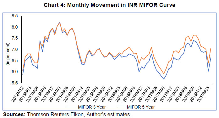
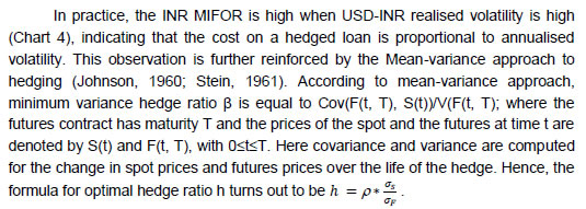 where, σs is the standard deviation of changes in spot prices over the life of the hedge, σF is the standard deviation of changes in future prices over the life of the hedge and ρ is the correlation coefficient between the two. From this formula (derivation provided in the Annex VI), it is evident that the optimal hedge ratio is proportional to the volatility of changes in the spot prices of the underlying. This stylised fact is a motivation for deriving an alternative optimal hedge ratio explained later (Methodology – Part II). This method being dependent on beta factor is not found stable over time (hedging horizon) and is restrictive in the sense that it could not be directly applied for multi- currency foreign portfolios. Moreover, basis risk arising due to imperfect matching between underlying assets and hedged assets (due to mismatches in maturity, liquidity and credit risk) is inherent in this method. IV. Data and Methodology Data Sources and Definitions The period of study in this paper is restricted to 2004-05: Q1 to 2018-19: Q3, which covers periods of the global financial crisis and the taper tantrum episode. Moreover, this period may be considered to be sufficient for establishing a long-term relationship in the ARDL formulation. IIP monthly data (base year 2011-12) was sourced from the Ministry of Statistics and Programme Implementation (MoSPI), Government of India website (http://www.mospi.gov.in). Non-food credit data was sourced from the Handbook of Statistics on the Indian Economy, Database on Indian Economy website (https://dbie.rbi.org.in) of Reserve Bank of India, which were converted into quarterly by taking month-end position of the respective quarters. Various rate variables in nominal term mentioned above like SPREAD (INR 3M MIBOR vs US 3M LIBOR / INR 5-year Treasury yield vs USD 5-year Treasury yield), INRLIQ (AAA rated INR 5-year corporate bond yield vs INR 5-year Treasury yield), USLIQ (AAA rated USD 5-year corporate bond yield vs USD 5-year Treasury yield) were sourced from Thomson Reuters Eikon and Bloomberg. The variable VOL (USD-INR realised volatility) with quarterly frequency was constructed from 30-day rolling volatility of USD-INR daily return (price of 1 Rupee). All exchange rate data, i.e., USD-INR, EUR-INR and JPY-INR were sourced from Thomson Reuters Eikon. Currency composition for ECBs portfolio was synthesised from currency composition of India’s External Debt statistics. While doing so, weight for the INR denominated debt was excluded and the remaining weight was normalised to one. Additionally, in this paper, seasonal adjustment census X-13 method was used for seasonal adjustment for the variables ECBs, IIP and NFC, where ever necessary. The paper investigates two empirical questions - firstly, what determines ECBs issuance in India, and secondly, what is the optimal hedging ratio? Accordingly, the paper adopts the following methodologies: Methodology – Part I In this section, an empirical model is estimated to ascertain the determinants of ECBs flow in India. The existing literature on the issuance of ECBs in India suggests that both domestic and global factors influence these flows. Though ECBs are in multi-currency, the US market is taken as a proxy of international market, representing the rest of the world for analysing the impact of spot exchange rate, international liquidity and interest rate arbitrage. From the domestic side, the following two real sectors/ financial variables are selected, viz., Index of Industrial Production (IIP) and Non-Food Credit (NFC). IIP is used as a proxy for domestic activity in the sense that ECBs are mainly raised by manufacturing and infrastructure firms. Most of the fund-use norms prescribed in the ECB guidelines are for domestic investment purposes. NFC is the major source of the flow of financial resources to commercial sectors in India (RBI Annual Report, various issues). When Indian banks are plagued with rising NPAs, corporates may take recourse to an alternative source of financing like ECBs. Hence, the variable NFC is used as a proxy for domestic liquidity/credit availability. The variable SPREAD (INR 5-year Treasury yield vs USD 5-year Treasury yield or alternatively, INR 3 Month MIBOR vs USD 3 Month LIBOR) is used to measure the scope for interest rate arbitrage. The variable INRLIQ (AAA rated INR 5-year corporate bond yield vs INR 5-year Treasury yield) is used to indicate domestic credit condition and liquidity. Similarly, the variable USLIQ (AAA rated USD 5-year corporate bond yield vs USD 5-year Treasury yield) is used as a proxy for international liquidity. The reasons behind taking 5-year benchmark yields include - (a) ECBs are long-term contracts and most of the issuances have a duration of 5 years, and (b) interest rate benchmark for ECBs issuance revolves around 5 years. USDINR (USD-INR spot exchange rate) and its realised volatility ‘VOL’ are also used in this study to see the corporates behaviour with respect to forex risk. In this study, a log-linear model is used by formulating the logarithm of ECBs issuance in terms of the logarithms of the IIP, non-food credit (NFC), USDINR (USD- INR exchange rates) and other rate variables like SPREAD (INR 3M MIBOR vs US 3M LIBOR or alternatively, INR 5-year Treasury yield vs USD 5-year Treasury yield ), INRLIQ (AAA rated INR 5-year corporate bond yield vs INR 5-year Treasury yield ), USLIQ (AAA rated USD 5-year corporate bond yield vs USD 5-year Treasury yield) and VOL (realised volatility of USD-INR spot exchange rate return). The following autoregressive distributed lag (ARDL) formulation by Pesaran and Shin (1999), which uses lagged terms of the dependent variable and contemporaneous as well as lagged terms of the exogenous regressors is used. The inclusion of lagged terms is justified as - (a) it is highly unlikely that current regressors could always affect ECBs issuance contemporaneously, (b) there could also be lagged responses induced by past contracts (Marquez, 2005), and (c) empirically, the variables considered above are a mixture of I (0) or I (1) processes: 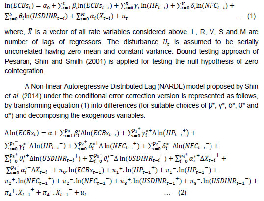 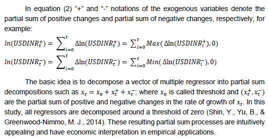 Shin et al. (2014) introduced the bound test for identifying asymmetrical cointegration in the long-run. The null hypothesis states that the effect is symmetrical in the long-run (H0: coefficients of the lagged level variables in the equation (2) are zero, simultaneously) against the alternative hypothesis that the coefficients of the lagged level variables are jointly non-zero. Methodology – Part II In this section, an innovative approach of using mean-variance optimisation framework is used to arrive at an optimal hedge ratio, which is important for a firm having multiple foreign-currency loans. Corporates having multi-currency exposures, often faced with the dilemma of whether to hedge each exposure and if so, by how much. Normally, they apply an ad hoc rule of hedging - either partially hedging or hedging those exposures for which contracts are favourable. This process ignores the correlation among exposures and hence may not lead to minimisation of the overall currency risk of the corporate. Instead, “a risk management best practice could be to compute the company’s total currency risk by using a portfolio’s FX Value at Risk (VaR) measure and determine a unique set of hedging ratios that minimize the company’s FX VaR for a specific level of total hedging cost”11. Following this, two separate optimisation exercises are described here. Optimization: Mean-Value-at-Risk approach V. Empirical Results V.1 Determinants of ECBs issuance V.1.1 Results based on application of a Linear ARDL model: Over the period 2004-05: Q1 to 2018-19: Q3, the IIP is found to have a statistically significant positive coefficient in short-run, implying that ECBs issuance are more when the domestic economic activity is high. In the long-run also, it has a statistically significant positive coefficient, reflecting that the growth in IIP acts as a domestic pull factor. Non-food credit has a positive coefficient, though not statistically significant, both in the short and long-run, indicating that the ECBs issuance were supplementing bank funding of the corporates. Nominal spread between INR 5-year Treasury yield and USD 5-year Treasury yield has a negative but statistically insignificant coefficient in the short-run as well as in the long-run, implying that the spread may not be contributing significantly to issuance of ECBs. However, over the sample period 2004: Q2 to 2017: Q4, that is after removing the recent calendar year 2018, the model reveals that in the short-run as well as in the long-run, the spread has a statistically significant positive coefficient. This analysis is supplemented by the recursive estimates of coefficients for the coefficient associated with spread, which remained in the positive territory till 2017: Q1 before turning negative with a clear mean reverting sign. (Annex-III: Recursive Coefficients). This situation is plausible in the sense that in 2018, interest rate arbitrage has gone down with comparatively high ECBs issuance, Chart 1. Thus, with declining spread arbitrage in the recent period, it is not a major factor driving issuance of ECBs. The extant ECB guideline is consistent with this fact since the ‘All-in-cost ceiling’ for issuing ECBs is LIBOR with 450 bps spread, irrespective of the tenor of the loan. The USD-INR spot exchange rate has a negative and statistically significant coefficient, meaning that the depreciation of INR vis-à-vis USD is contributing negatively in issuance of ECBs. INRLIQ, i.e., spread between INR AAA rated 5-year corporate bond yield and INR 5-year Treasury yield is found to contribute positively to issuance of ECBs since it has a positive and statistically significant coefficient. If this spread is more, it implies that Indian corporates are not able to raise funds in the local capital market at competitive yield by issuing corporate bonds and hence they are taking recourse to an alternative route like ECB. USLIQ, i.e., spread between USD AAA rated 5-year corporate bond yield and USD 5-year Treasury yield has a negative and statistically significant coefficient, implying that the USLIQ is contributing to the issuance of ECBs. The USD-INR exchange rate volatility having a positive (hovering close to zero) and statistically significant coefficient in the long-run, appears to be counter-intuitive. To study this in greater detail, recursive estimates of this coefficient are generated (Annex III: Recursive Coefficients). It is found that in times of excessive volatility as during the taper tantrum, this coefficient was negative. In the short-run, realised volatility does not have a statistically significant coefficient. Over the sub period of study 2012: Q2 to 2018: Q412, long-run form and bound test of ARDL model reveals that it is mainly USD-INR depreciation which has led to moderation in the issuance of ECBs as it has negative and statistically significant coefficient. Other factors contributing to the issuance of ECBs are IIP and USD-INR volatility. V.1.2 Results based on application of a Non-linear ARDL model: Assuming that the cyclical upturns and downturns in the macroeconomic variables would have an asymmetrical impact on issuance of ECBs, a Non-linear Autoregressive Distributed Lag (NARDL) model following Shin & others (2014) (building on the linear ARDL model) was estimated. In this model non-linearity is measured by evaluating the asymmetric impact of regressors (i.e., IIP, non-food credit, USD-INR spot rate, SPREAD, INRLIQ, USLIQ, USD-INR exchange volatility ‘VOL’) on the issuance of ECBs. Under this set up, all these variables are decomposed into two parts which are a cumulative sum of positive changes and a cumulative sum of negative changes. Thus, seven independent variables are decomposed into 14 series to study their asymmetric impact on the issuance of ECBs during 2004: Q2 to 2018: Q4. ARDL/Non-linear ARDL can generate statistically significant results even with small sample size (unlike Johansen cointegration method which requires a larger sample size to attain significance). It revealed statistically significant asymmetric impact of majority of 14 regressors. However, the error correction coefficient was in the range [0.99, 1.16] for various models (though with negative sign and statistically significant). To resolve this issue, a modified formulation was estimated. From linear ARDL, it was evident that the variables INRLIQ and VOL had small coefficients; hence, these variables were not decomposed, but were augmented as regressors, while adopting a Non-linear ARDL model. The regressor SPREAD (a measure of interest rate arbitrage) also had a small coefficient. However, since this variable is an important determinant of ECBs issuance, it was decomposed into partial sum of positive and negative changes. The real sector variable IIP was just augmented as a regressor in the Non-linear ARDL model (used without decomposing it). Based on this formulation, following results are obtained: V.1.3 For the variables which were not decomposed: Growth in IIP is contributes positively to ECBs issuance in the long-run which is consistent with the finding of Linear ARDL. Similarly, INRLIQ has a positive impact on issuance of ECBs in the long-run. Increase in the exchange rate volatility has an adverse impact in the short-run, though the size of its coefficient is very low and statistically insignificant. V.1.4 For the variables which were decomposed: Negative changes in SPREAD (a decrease in spread) has an asymmetric negative impact on issuance of ECBs in the short-run as well in the long-run and is statistically significant at the 10 per cent level of significance. Positive changes in SPREAD confirms in sign and thus, contributing in issuance of ECBs. However, it is not statistically significant. Moreover, the size of the coefficient of positive changes in SPREAD is remarkably lower. Thus, ECBs issuance respond more asymmetrically to negative shocks to the spread than to positive shocks. When depreciation is separated from appreciation under the Non-linear ARDL estimation, it is observed that the INR depreciation vis-a-vis USD has a significant adverse impact in the short-run as well as in the long-run in issuance of ECBs. However, INR appreciation vis-a-vis USD has a positive impact (though statistically insignificant) in the short-run while in long-run, it has a negative impact (though statistically insignificant). Thus, the exchange rate does have an asymmetric adverse impact. The Non-linear ARDL model revealed existence of an asymmetric effect of non-food credit. In the short-run, ECBs issuance react more strongly to negative changes in non-food credit, as the size of its coefficient is larger and statistically significant at the 10 per cent level of significance. The partial sum of positive changes in non-food credit has a negative coefficient (though statistically insignificant) in the short-run. However, in the long-run there is a reversal in sign of the coefficients (though statistically insignificant). Thus, there is a switching in the direction of asymmetry (though statistically insignificant) between short-run and long-run. The asymmetric behaviour is also observed in case of international liquidity, as measured by the variable USLIQ. In the short-run, higher international liquidity leads to higher ECBs issuance. In the long-run, one unit positive or negative change has a similar impact though the coefficient of unit negative changes (availability of high liquidity) has a larger size (statistically significant coefficient). This implies higher international liquidity leads to higher ECBs issuance. The model was validated with all diagnostics and stability tests and found stable. V.2 Optimal Hedge Ratio computation Post global financial crisis period was marked with high volatility when central banks as well as corporates were more concerned about forex vulnerability. On the one hand, banks and policymakers would be more comfortable if all the forex exposures were financially hedged. On the other hand, corporates undertaking hedging contracts for their forex exposure would be looking for a trade-off between hedging cost and forex risk. This is because, in times of high volatility, as was the case during the taper tantrum in 2013, hedging cost increases enormously and the trade-off becomes more challenging. During the taper tantrum (May-September 2013), INR MIFOR curve was in a range (6.4 per cent to 7.6 per cent); however, it was high at 8.2 per cent in March 2014 (Chart 4). Similarly, during June-December 2018 when realised volatility was in the range (6.5 per cent to 7.8 per cent), INR MIFOR ranged between (7.14 per cent to 7.54 per cent). Assuming that the major currencies in which ECBs were issued are USD, EUR and JPY, the currency composition for the ECBs portfolio was synthesised by using the currency composition of India’s external debt (Annex II: Table 4). For this purpose, total weight was normalised to one, by ignoring INR and other small currencies. Thus, the synthesised ECBs portfolio (USD, EUR, JPY) has the weight as (86 per cent, 6 per cent, 8 per cent, respectively). (Annex II: Table 4). The variance-covariance matrix of daily return of (USD-INR, EUR-INR, JPY-INR) is computed for May to November 2013 (which covers the stressed period of the taper tantrum episode13) and then annualised by multiplying it by 252. Ideally, the length of time interval should be the same as that of the time interval for which hedge is in effect. However, it severely limits the number of available observations hence daily return data are used. The aim of this exercise is to assess the total FX risk of ECBs portfolio (USD, EUR, JPY) by computing FX Value at Risk (VaR) and then determining a hedge ratio that minimises the ECBs portfolio FX VaR for a given hedging cost (cost on a hedged loan). For the ECBs portfolio (USD=86 per cent, EUR=6 per cent, JPY=8 per cent), hedging cost is assumed to be proportional to the weighted volatility which comes out to 13.99 per cent during May to November 2013. An optimisation exercise for minimising the ECBs portfolio parametric linear VaR, to reduce the hedging cost to a level 8.95 per cent, leads to 37 per cent reduction in FX VaR, and requires 63.14 per cent of the ECBs portfolio with a portfolio composition (USD=49.14 per cent, EUR=6 per cent, JPY=8 per cent) to be hedged either financially or naturally. Similarly, if the hedging cost is reduced from 13.99 per cent to half, i.e., 6.99 per cent (implying that volatility has gone down drastically), 48.80 per cent of ECBs portfolio with portfolio composition (USD=34.80 per cent, EUR=6 per cent, JPY=8 per cent) is required to be hedged and it would lead to a reduction in portfolio FX VaR by 51.13 per cent. Alternatively, one may apply a rule of thumb to hedge simply half of each of the exposure, if the aim is to reduce the cost by half. However, such a strategy would ignore FX risk of the portfolio. On the other hand, if one attempt to minimise the cost of hedging, fixing FX VaR to a level, say two third of unhedged portfolio FX VaR, requires 66.12 per cent of ECBs portfolio with a portfolio composition (USD=66.12 per cent, EUR=0 per cent, JPY=0 per cent) to be hedged, with a minimum cost of hedging achieved at 9.04 per cent. In the above optimisation framework, the required cost on a hedged loan is assumed to be nearly 9 per cent and 7 per cent. The reason behind using these rates as plausible scenarios may be attributed to - (1) an estimated implicit interest rate on ECBs (interest payments based on terms of borrowings during the year as a percentage of the outstanding debt at the end of the previous year) of 4.7 per cent (India’s External Debt statistics-A Status Report 2016-17). This implicit cost may be supplemented/ compounded with the fact that the average annual INR depreciation post global financial crisis was around 4.5 per cent (Annex IV: Chart 6); and (2) INR MIFOR curve touched a level more than 8 per cent during the taper tantrum. The possibility of sourcing ECBs at equivalent INR cost less than the prevailing G-sec yield of nearly 5.95 per cent is ignored in this analysis. To sum up, in times of typical high FX volatility, firms issuing ECBs may take recourse to hedge their exposure financially/naturally in the range [63 per cent, 66 per cent], which would translate to the total cost on loan, including hedging cost, proportional to nearly 9 per cent. Moreover, this strategy is likely to lead to protection against forex risk, as FX VaR reduces by 33 per cent. VI. Conclusion It has been observed that many Indian firms augment local banking sources for raising funds with recourse to ECB route, thereby diversifying their debt profile. After the global financial crisis, there was a surge in capital flows to emerging markets. This phenomenon created scope for interest rate arbitrage as the policy interest rates in developed markets moved to near zero. Over time such arbitrage benefit has diminished sharply, leading to a moderation in ECBs issuance. However, due to major policy liberalization albeit with certain restrictions in January 2019, ECBs issuance staged at a historically highest level of USD 53 billion in 2019-20. Expectation of the rupee depreciation had an adverse impact on the issuance of ECBs. Large and lumpy principal repayments liability may arise during a short span of time on account of ECBs borrower which if unhedged may lead to domestic forex market susceptible to bouts of excessive volatility. Given the interest rate differential between India and the developed markets, all foreign currency exposures carry a significant cost of hedging. Hedging all FX exposures in their entirety may not be optimal in the sense that with fully hedged FX exposure, the benefit of low-cost access to foreign capital is foregone and at the same time unhedged foreign currency exposures may lead to correlated defaults in debt servicing triggering build-up of systemic risk. Therefore, there is a need to understand the optimal hedge ratio as may be discerned from empirical estimation for a minimum variance hedge ratio. This study finds that the optimal hedging ratio either financial or natural hedge at a system level may be in the vicinity of 63 per cent, though as the strategy in practice could be time varying a somewhat higher ratio may be useful in periods of expected stress. Also, firms may need to consider the dynamic hedging strategy on firm specific and sector specific considerations as well. From a macro-viewpoint with outstanding ECBs in the vicinity of 6.5 per cent of nominal GDP, they constitute close to 30 per cent of India’s external debt. Therefore, from the standpoint of maintaining macro-financial stability, it is prudent to have a judicious policy on optimal hedge ratios.
References Article-IV Consultation (2018) IMF Staff Report for India, Country report no 18/254. Acharya, V. V., & Vij, S. (2020). Foreign currency borrowing of corporations as carry trades: Evidence from India. NBER Working Paper, w28096. Annual Report of the Reserve Bank of India, various issues. Article by FX Market Specialist Gorelik, Matt (2016). Hedge ratio optimization helps keep FX risks and costs low. Bloomberg Briefs. Bakardzhieva, D, Ben Naceur, S and Kamar, B (2010). The Impact of Capital and Foreign Exchange Flows on the Competitiveness of Developing Countries. IMF working paper, WP/10/154. Hoggarth & Sterne (1997). Capital flows: Causes, Consequences and Policy Responses. CCBS Handbooks in Central Banking. India’s External Debt statistics-A Status Report 2016-17 & 2017-18. Johnson, L. L. (1960). The theory of hedging and speculation in commodity futures. The Review of Economic Studies, 27:139-151. Marquez, Jaime (2005). Estimating elasticities for U.S. trade in services. Elsevier, Economic Modelling 23: 276– 307. Mohanty, M. S. and Sundaresan, Suresh (2018). FX Hedging & Creditor Rights. BIS, Papers No 96b. Patnaik, I., Shah, A., and Singh, N. (2016). Foreign Currency Borrowing by Indian Firms. India policy forum (139-174), NIPFP. Pesaran MH, Shin Y. (1999). An autoregressive distributed lag modelling approach to cointegration analysis. Chapter 11 in Econometrics and Economic Theory in the 20th Century. The Ragnar Frisch Centennial Symposium, Strom S (ed.). Cambridge University Press, Cambridge. Pesaran, MH, Shin, Y., & Smith, R. (2001). Bound testing approaches to the analysis of level relationships. Journal of Applied Econometrics, 16(3): 289–326. Ray, Partha et. al. (2017). India’s External Commercial Borrowing: Trends, Composition and Determinants. Indian Institute of Management, Calcutta, WPS No.802. Report on Currency and Finance (2004-05), Reserve Bank of India. Shin, Y., Yu, B., & Greenwood-Nimmo, M. J. (2014). Modelling asymmetric cointegration and dynamic multipliers in a nonlinear framework. In Williams C. Horrace, & Robin C. Sickles (Eds.), Festschrift in honor of Peter Schmidt. Econometric methods and applications New York (NY): Springer, Science & Business Media, New York, 2014, pp. 281–314. Singh, Bhupal (2007). Corporate Choice for Overseas Borrowing: The Indian Evidence. Reserve Bank of India Occasional Papers, 28(3): Winter. Singh, Bhupal (2009). Changing Contours of Capital Flows to India. Economic and Political Weekly, VOL XLIV No. 43. Stein, J. L. (1961). The simultaneous determination of spot and futures prices. The American Economic Review, 51(5): 1012-1025. The Clearing Corporation of India Limited Monthly Newsletter, Rakshitra, March 2019. Verma, Radheshyam and Prakash, Anand (2011). Sensitivity of Capital Flows to Interest Rate Differentials: An Empirical Assessment for India. RBI Working Paper Series, WPS (DEPR): 7/2011.
Annex I | Table I.1: Variable Description and a priori expectation on the sign of coefficients | | Variables | Description | Hypothesis | | ECB_RF | External Commercial Borrowings excluding refinancing of earlier loans | - | | IIP | Index of Industrial Production | Positive | | NFC | Non-food Credit | Positive/Negative | | INRLIQ | AAA rated INR 5 year corporate bond yield vs INR 5 year Treasury yield | Positive | | SPREAD | INR 5 year Treasury yield vs USD 5 year Treasury yield or alternatively, INR 3 Month MIBOR vs USD 3 Month LIBOR | Positive | | USDINR | Spot exchange rate | Negative | | USLIQ | AAA rated USD 5 year corporate bond yield vs USD 5 year Treasury yield | Negative | | VOL | Spot USD-INR realised volatility | Negative | | Source: Author’s proposition. |
| Table I.2: Results of Unit Root Test for Stationarity - period 2004Q2 2018Q4 | | Variables | Augmented Dickey Fuller Test | Phillips Perron Test | | t-stat | p-value | Order of integration | t-stat | p-value | Order of integration | | ECB_RF | -4.27 | 0.00 | I(0) | -4.15 | 0.00 | I(0) | | IIP | -3.05 | 0.13* | I(1) | -11.89 | 0.00* | I(1) | | NFC | -11.12 | 0.00 | I(1) | -10.95 | 0.00 | I(1) | | INRLIQ | -7.13 | 0.00 | I(1) | -7.87 | 0.00 | I(1) | | SPREAD | -9.35 | 0.00 | I(1) | -9.39 | 0.00 | I(1) | | USDINR | -7.24 | 0.00 | I(1) | -7.26 | 0.00 | I(1) | | USLIQ | -6.64 | 0.00 | I(1) | -6.57 | 0.00 | I(1) | | VOL | -4.52 | 0.00 | I(0) | -4.52 | 0.00 | I(0) | Note: I(k) means the series is integrated of order k. ‘Trend & Intercept’ is taken in Test Equation, for ‘*’ marked cases. Unit root tests for the period 2012Q2 to 2018Q4 also show that all series are either I(0) or I(1).
Source: Author’s estimates. |
Annex II | Table II.1: ARDL Models for ECBs issuance | | Variables | Overall 2004Q2 2018Q4:
ARDL(1, 0, 0, 0, 2, 1, 1, 2) | 2012Q2 2018Q4:
ARDL(1, 1, 0, 0, 2, 1, 2, 2) | | Coeff. | t-Stat | P-value | Coeff. | t-Stat | P-value | | LOG(ECB_RF_D11(-1)) | 0.14 | 1.08 | 0.29 | 0.08 | 0.61 | 0.56 | | LOG(IIP_D11) | 2.06 | 4.16 | 0.00 | -2.03 | -0.43 | 0.68 | | LOG(IIP_D11(-1)) | | | | 8.27 | 1.96 | 0.07 | | LOG(NFC_D11) | 2.18 | 1.18 | 0.25 | 3.70 | 1.69 | 0.12 | | SPREAD | -0.05 | -1.14 | 0.26 | -0.02 | -0.39 | 0.70 | | LOG(USDINR) | -0.33 | -0.33 | 0.75 | -2.16 | -1.33 | 0.21 | | LOG(USDINR(-1)) | 1.64 | 1.18 | 0.24 | 1.08 | 0.51 | 0.62 | | LOG(USDINR(-2)) | -2.91 | -3.11 | 0.00 | -4.14 | -1.75 | 0.11 | | INRLIQ | 0.08 | 0.58 | 0.56 | -1.32 | -2.77 | 0.02 | | INRLIQ(-1) | 0.41 | 3.04 | 0.00 | 0.92 | 2.06 | 0.06 | | USLIQ | -0.65 | -1.86 | 0.07 | 1.18 | 2.26 | 0.05 | | USLIQ(-1) | -0.94 | -3.05 | 0.00 | -1.39 | -1.89 | 0.08 | | USLIQ(-2) | | | | -0.98 | -1.78 | 0.10 | | VOL | 0.002 | 0.35 | 0.73 | 0.02 | 0.94 | 0.37 | | VOL(-1) | 0.01 | 1.14 | 0.26 | 0.01 | 0.40 | 0.70 | | VOL(-2) | 0.03 | 2.20 | 0.03 | 0.07 | 4.74 | 0.00 | | C | 4.20 | 2.46 | 0.02 | | | | | CointEq(-1) | -0.86 | -7.62 | 0.00 | -0.92 | -8.77 | 0.00 | | | Adj. R2=0.60, DW=2.13, F=7.03,
Bounds test =6.22*** | Adj. R2=0.69, DW=2.20,
Bounds test = 5.88*** | Note: *** represents statistical significance at 1%.
Source: Author’s estimates. |
| Table II.2: Long-run Coefficients of ECBs Issuance | | | Overall 2004Q2 2018Q4:
ARDL(1, 0, 0, 0, 2, 1, 1, 2) | 2012Q2 2018Q4:
ARDL(1, 1, 0, 0, 2, 1, 2, 2) | | Variables | Coeff. | t-Stat | P-value | Coeff. | t-Stat | P-value | | LOG(IIP_D11) | 2.40 | 3.76 | 0.00 | 6.78 | 7.74 | 0.00 | | LOG(NFC_D11) | 2.53 | 1.12 | 0.27 | 4.01 | 1.68 | 0.12 | | SPREAD | -0.06 | -1.09 | 0.28 | -0.02 | -0.38 | 0.70 | | LOG(USDINR) | -1.85 | -3.85 | 0.00 | -5.67 | -5.63 | 0.00 | | INRLIQ | 0.58 | 3.00 | 0.00 | 0.43 | -1.18 | 0.26 | | USLIQ | -1.85 | -7.51 | 0.00 | -1.29 | -1.20 | 0.26 | | VOL | 0.06 | 2.19 | 0.03 | 0.10 | 5.56 | 0.00 | | Source: Author’s estimates. |
| Table II.3: Annualised Variance-covariance matrix of Forex return for the period May November 2013 | | (In per cent) | | Variance-Covariance Matrix | USD/INR | EUR/INR | JPY/INR | | USD/INR | 1.87 | 1.65 | 1.78 | | EUR/INR | 1.65 | 1.97 | 1.96 | | JPY/INR | 1.78 | 1.96 | 3.05 | | Volatility | 13.66 | 14.04 | 17.46 | | Source: Author’s estimates. |
| Table II.4: Synthesised Currency Composition for ECBs | | Major Currencies | External Debt Currency composition as on end March 2018 (in %)* | Synthesised currency composition for ECBs (in %) | | USD | 49.50 | 86 | | EUR | 3.40 | 6 | | JPY | 4.70 | 8 | | INR | 35.80 | - | | Others** | 6.60 | - | | Total | 100 | 100.00 | Note: ** - Others includes SDR (5.50%), Pound Sterling (0.60%) & other small currencies (0.50%).
Sources: Report on INDIA’S EXTERNAL DEBT 2017-18, Author’s estimates. |
Annex-III
Annex IV
Annex V Major changes in the recent ECB framework: • 2015: Security/ guarantee provisions for raising ECB was relaxed. Liberalised framework for Rupee denominated bonds (Masala bonds/RDB) was introduced in September 2015. ECB framework was revised with some restrictions on end-uses, higher all-in-cost ceiling for longer-term borrowing, etc. Three distinct tracks for borrowing, viz., Track-I for medium-term foreign currency borrowing, Track-II for long-term foreign currency borrowings and Track-III for INR denominated ECBs was created. List of recognised lenders was also expanded with long-term investors like sovereign wealth funds, pension funds, etc., under the revised ECB framework along with removal of limit for prepayment under auto route which complied with minimum average maturity norms. Indian banks were prohibited from refinancing of ECBs due to prudential concerns. Parking of ECB proceeds, pending utilisation, in fixed deposits in India was permitted for 12 months (from 6 months). • 2016: ECB facility for working capital by airlines companies, ECB facility for low cost affordable housing and USD 10 bn schemes got discontinued from March 31, 2016. Infrastructure sector companies and companies financing infrastructure were permitted to raise ECB having maturity of less than 10 years, only with 100 per cent hedging. RDB was permitted to be raised by Indian banks. Required maturity for issuing RDB was reduced to 3 years. RDB was brought within aggregate limit of FPI investment in corporate bonds. Framework of ECB for Startups was also released. • 2017: Maturity period of RDB got aligned with ECBs, all-in-cost ceiling for RDB was introduced, related parties were excluded from recognised investors and aggregate limit provision dispensed with, for RDB. • 2018: Permitted the overseas branches/subsidiaries of Indian banks to refinance ECBs of highly rated (AAA) corporates as well as Navratna and Maharatna PSUs. • Rationalisation of all-in-cost ceiling of 450 basis points over benchmark rate and end-use purposes for ECB under all tracks, increasing the ECB liability: equity ratio from 4:1 to 7:1 in automatic route and expansion of eligible borrowers list for the purpose of ECB. • As per revised guideline “minimum average maturity (MAM) was decreased from 3 years to 1 year for ECB up to USD 50 million or its equivalent for manufacturing sector. Permitted Indian banks to participate as arrangers/underwriters/market makers/traders in RDBs issued overseas subject to applicable prudential norms”. • ECB guideline allowed “Public Sector Oil Marketing Companies (OMCs) to raise ECB for working capital purposes with MAM period of 3/5 years, respectively, from all recognized lenders under the automatic route without mandatory hedging requirements with overall ceiling of USD 10 billion or equivalent”. • It also “reduced the average maturity requirement from 10 years to 5 years for exemption from mandatory hedging provision for infrastructure sector. ECBs with MAM of 3 to 5 years in the infrastructure space with 70% mandatory hedging requirement was introduced”.
Annex VI Derivation of Hedge ratio in the portfolio context Consider a portfolio Y with weights (w, 1-w), as a linear combination of two securities A and B for which expected return and variance exists such that: Suppose we have exposure in $1 of Security A, and we wish to hedge it with $h of Security B (if h is positive, we are buying the security and if h is negative, we are shorting the security). In other words, h is the hedge ratio. If P (1, h) is our hedged portfolio, such that P= A + hB, then, using the above expression for the portfolio variance, hedged portfolio variance is The minimum variance hedge ratio is ratio which would achieve the portfolio with the least variance. It is found by taking the partial derivative of the equation for the portfolio variance with respect to h, and setting it equal to zero such that: h = ±ρAB*σA/σB. For maxima or minima, one needs to see the sign of double derivative.
Annex VII Some Previous Studies relating to External Commercial Borrowings in India | Study | Main findings | | Singh, Bhupal (2007) | Attempted to find the long-run demand for ECBs by error correction model based on quarterly data from April 1993 to March 2007. It was found “the Indian corporates’ long-run demand for overseas commercial borrowings is predominantly influenced by the pace of domestic real activity, followed by the interest rate differentials between the domestic and international markets (indicating arbitrage) and the credit condition”. | | Singh, Bhupal (2009) | - “Analysed the determinants of various components of private debt flows and equity flows to India. It was found that there exists a high correlation between ECB disbursements and interest rate differential (i.e., the commercial banks’ prime lending rate minus the six-month LIBOR). It also observed strong co-movement of ECBs and domestic activity”.
- “It found that Indian corporates’ long-run demand for overseas commercial borrowings is predominantly influenced by the pace of domestic real activity, followed by interest rate differentials and the credit conditions in domestic markets”.
- “During normal periods, the overseas borrowings are influenced by the underlying domestic demand shocks, the external credit shocks seem to be the most dominant factor during the periods of financial crisis”.
- Using the model vector error correction (VEC) with monthly data for the period 1993:1 to 2009:3, it found “NRI deposits are significantly influenced by real economic activity in the host country (index of oil price was taken as a proxy), exchange rate movements and interest rate differential”.
| | Bakardzhieva, D, Ben Naceur, S and Kamar, B (2010) | - Investigated the impact of different types of capital and foreign exchange flows on real exchange rate behavior in 57 developing countries covering Africa, Europe, Asia (India was included in the sample), Latin America, and the Middle East.
- It found “portfolio investments, foreign borrowing, aid, and income lead to real exchange rate appreciation”.
| | Verma, Radheshyam and Prakash, Anand (2011) | “Provided empirical evidence of sensitivity of capital inflows to interest rate differential in India; specific context that debt creating flows, in particular ECBs, FCNR(B) and NR(E)RA deposits exhibit statistically significant sensitivity to interest rate differentials, even though other determinants of these inflows dominate significantly the impact of interest rate differential”. | | Patnaik at el. (2015) | Highlighted the systemic risk on account of unhedged Foreign Currency borrowings by the Indian corporates. | | Acharya, Viral V and Vij, Siddharth (2020)* | - Tested the hypothesis that issuance propensity for the firm is higher when the dollar 'carry trade' is favorable by using firm level logit model. In contrast, most standard firm-level variables, on their own, are not predictive of ECBs issuance. Macroprudential policies by regulators are helpful in managing such capital flows.
- They also tested the hypothesis that the firm’s cash balances rise more after a foreign currency debt is issued and firm’s exposure to foreign exchange risk rises after an issuance implying that the currency risk is not fully hedged.
- Highlighted difference between market based risk measure versus accounting measures. Using the 'taper tantrum' episode of Summer 2013 as stressed period to foreign exchange volatility, they found that a market-based measure of FX exposure such as Forex-beta does a better job in capturing firm exposures than accounting measures/ratios.
| | Ray, Partha et. al. (2017) | “Investigated the role of domestic and global factors in influencing the ECB flows to India. Results suggest that both the domestic and international factors have significantly influenced ECB flows to India. They found exchange rate fluctuations as a major risk of foreign currency borrowings. Similar to other studies, they found that the interest rate differential and growth differential are also influencing ECB flows in India. They have also found a negative relationship between International liquidity and ECBs flow, which seems to be counter intuitive, however, authors have explained this finding in the light of restrictive measures adopted by the Reserve Bank to regulate capital inflows, time to time”. | | Mohanty and Sundaresan (2018) | Explored the impact of bankruptcy law and bankruptcy code on firm’s forex hedging behavior. When the bankruptcy code is weak in protecting the rights of creditors, value maximizing firms hedge a higher proportion of the value of their assets at the time debt is issued. Forex exposure affects credit spreads and thin forex hedging market lead to greater forex exposure, and a higher probability of default. Focused on India’s new bankruptcy law, study found that the new bankruptcy law in India has a positive impact on the hedging behavior of Indian firms. | | *Highlights of Acharya, Viral V and Vij, Siddharth study presented here is majorly from their paper presented in the NSE-NYU Conference on Indian Financial Markets, 2017. |
ANNEX VII Residual Diagnostics of Linear ARDL (using EViews 10): | Heteroskedasticity Test: Breusch-Pagan-Godfrey | | Null hypothesis: Homoskedasticity | | F-statistic | 1.240593 | Prob. F(14,42) | 0.2841 | | Obs*R-squared | 16.67545 | Prob. Chi-Square(14) | 0.2739 | | Scaled explained SS | 7.162415 | Prob. Chi-Square(14) | 0.9283 | | Source: Author’s estimates. |
| Breusch-Godfrey Serial Correlation LM Test | | Null hypothesis: No serial correlation at up to 2 lags | | F-statistic | 0.311640 | Prob. F(2,40) | 0.7340 | | Obs*R-squared | 0.874547 | Prob. Chi-Square(2) | 0.6458 | | Source: Author’s estimates. |
ANNEX VIII Stability Diagnostics of Linear ARDL: | Ramsey RESET Test | | Equation: EQ01 | Specification: LOG(ECB_RF_D11) LOG(ECB_RF_D11(-1)) LOG(IIP_D11)
D(LOG(NFC_D11) SPREAD LOG(USDINR) LOG(USDINR(-1)) LOG(USDINR(-2)) INRLIQ INRLIQ(-1) USLIQ USLIQ(-1) VOL VOL(-1) VOL(-2) C | | Omitted Variables: Squares of fitted values | | | Value | Df | Probability | | t-statistic | 1.362209 | 41 | 0.1806 | | F-statistic | 1.855612 | (1, 41) | 0.1806 | | Likelihood ratio | 2.523079 | 1 | 0.1122 | | Source: Author’s estimates. |
ANNEX IX Non-linear auto-regressive distributed lag (NARDL) model application: | Table IX.1: Variable Description and a priori expectation on the sign of coefficients | | Variables | Description | Hypothesis | | ECB_RF | External Commercial Borrowings excluding refinancing of earlier loans | - | | LIIP_POS | Partial sum process of positive changes in the growth of logarithmic Index of Industrial Production | Positive | | LIIP_NEG | Partial sum process of Negative changes in the growth of logarithmic Index of Industrial Production | Positive | | LNFC_POS | Partial sum process of positive changes in the growth of logarithmic Non-food Credit | Positive/Negative | | LNFC_NEG | Partial sum process of negative changes in the growth of logarithmic Non-food Credit | Negative/Positive | | SPREAD_POS | Partial sum process of positive changes in the spread of INR 5 year Treasury yield vs USD 5 year Treasury yield | Positive | | SPREAD_NEG | Partial sum process of negative changes in the spread of INR 5 year Treasury yield vs USD 5 year Treasury yield | Positive | | LEX_POS | Partial sum process of positive changes in the growth of logarithmic USD/INR Spot exchange rate | Negative | | LEX_NEG | Partial sum process of negative changes in the growth of logarithmic USD/INR spot exchange rate | Negative | | INRLIQ | AAA rated INR 5 year corporate bond yield vs INR 5 year Treasury yield | Positive | | USLIQ_POS | Partial sum process of positive changes in the spread of AAA rated USD 5 year corporate bond yield vs USD 5 year Treasury yield | Negative | | USLIQ_NEG | Partial sum process of negative changes in the spread of AAA rated USD 5 year corporate bond yield vs USD 5 year Treasury yield | Negative | | VOL | Spot USD-INR realised volatility | Negative |
| Table IX.2: Dynamic asymmetric estimation of ECBs issuance | | Sample 2004Q2 2018Q4: | NARDL (1, 1, 1, 1, 0, 0, 0, 1, 1, 1, 0, 1) | | Variables | Coeff. | t-Stat | P-value | | LOG(ECB_RF_D11(-1)) | 0.13 | 1.21 | 0.23 | | LIIP | -1.85 | -0.84 | 0.40 | | LIIP(-1) | 3.34 | 1.55 | 0.13 | | LNFC_POS | -1.70 | -0.54 | 0.59 | | LNFC_POS(-1) | 3.11 | 1.48 | 0.15 | | LNFC_NEG | 4.20* | 1.74 | 0.09 | | LNFC_NEG(-1) | -6.52** | -2.07 | 0.05 | | SPREAD_POS | 0.04 | 1.09 | 0.28 | | SPREAD_NEG | 0.09* | 1.82 | 0.08 | | LEX_POS | -1.95*** | -2.85 | 0.01 | | LEX_NEG | -1.32 | -0.47 | 0.64 | | LEX_NEG(-1) | 3.86 | 1.23 | 0.22 | | INRLIQ | 0.04 | 0.36 | 0.72 | | INRLIQ(-1) | 0.42** | 2.22 | 0.03 | | USLIQ_POS | 0.92 | 1.56 | 0.13 | | USLIQ_POS(-1) | -2.69*** | -3.68 | 0.00 | | USLIQ_NEG | -2.00*** | -5.87 | 0.00 | | VOL | -0.0006 | -0.05 | 0.96 | | VOL(-1) | 0.04*** | 3.69 | 0.00 | | CointEq(-1) | -0.87*** | -9.06 | 0.00 | | Adj. R2=0.66, DW=2.14, F=5.27, Bounds test =3.6*** | Note: ***, ** & * represent statistical significance at 1%, 5% & 10% levels, respectively.
Source: Author’s estimates. |
| Table IX.3: Asymmetric long-run Coefficients of ECBs issuance | | Levels Equation: No constant and No Trend | | Variables | Coefficient | t-Stat | P-value | | LIIP | 1.71 | 30.49 | 0.00 | | LNFC_POS | 1.62 | 0.32 | 0.75 | | LNFC_NEG | -2.66 | -0.49 | 0.63 | | SPREAD_POS | 0.05 | 1.07 | 0.29 | | SPREAD_NEG | 0.11 | 1.92 | 0.06 | | LEX_POS | -2.23 | -2.75 | 0.01 | | LEX_NEG | 2.91 | 1.52 | 0.14 | | INRLIQ | 0.53 | 2.90 | 0.01 | | USLIQ_POS | -2.04 | -10.28 | 0.00 | | USLIQ_NEG | -2.29 | -7.19 | 0.00 | | VOL | 0.04 | 1.93 | 0.06 | | Source: Author’s estimates. |
ANNEX X Residual Diagnostics for NARDL (using EViews 10): | Heteroskedasticity Test: Breusch-Pagan-Godfrey | | Null hypothesis: Homoskedasticity | | F-statistic | 0.9533 | Prob. F(14,42) | 0.5304 | | Obs*R-squared | 18.7449 | Prob. Chi-Square(14) | 0.4733 | | Scaled explained SS | 7.4805 | Prob. Chi-Square(14) | 0.9912 | | Source: Author’s estimates. |
| Breusch-Godfrey Serial Correlation LM Test | | Null hypothesis: No serial correlation at up to 2 lags | | F-statistic | 0.780459 | Prob. F(2,40) | 0.4660 | | Obs*R-squared | 2.390842 | Prob. Chi-Square(2) | 0.3026 | | Source: Author’s estimates. |
ANNEX XI Stability Diagnostics NARDL: | Ramsey RESET Test | Specification: LOG(ECB_RF_D11) LOG(ECB_RF_D11(-1)) LIIP LIIP(-1) LNFC_POS LNFC_POS(-1) LNFC_NEG LNFC_NEG(-1) SPREAD_POS SPREAD_NEG LEX_POS
LEX_NEG LEX_NEG(-1) INRLIQ INRLIQ(-1) USLIQ_POS USLIQ_POS(-1) USLIQ_NEG VOL VOL(-1) | | Omitted Variables: Squares of fitted values | | | Value | df | Probability | | t-statistic | 0.105395 | 36 | 0.9166 | | F-statistic | 0.011108 | (1, 36) | 0.9166 | | Likelihood ratio | 0.017277 | 1 | 0.8954 | | Source: Author’s estimates. |
|