Press Release

RBI Working Paper Series No. 04

States’ Fiscal Performance and Yield Spreads on Market Borrowings in India

Ramesh Jangili, N.R.V.V.M.K. Rajendra Kumar and Jai Chander^@

Abstract

^*State governments are borrowing significantly from the market to meet their budgetary requirements. As investors are risk-conscious, fiscal fundamentals may impact the yields, and states’ borrowing costs. Indicator-based assessment of the states’ performance is cumbersome, keeping in view a large number of indicators. Therefore, we develop a holistic measure of the states’ performance by developing a composite index that incorporates fiscal, debt and market-related indicators. We empirically find that the index has a statistically significant relationship with the yield spreads, which suggests that better performance of states is rewarding as it lowers borrowing costs. The index can also be used by investors to make more informed investment decisions, which in turn, can enhance the efficiency of the price discovery mechanism of state government securities in India.

JEL Classification: H74, H70, C43, C23, G12

Keywords: States’ performance, market borrowings, yield spreads, composite index, panel regression

Introduction

Over the years, the financing pattern of the state governments’ fiscal deficit has changed significantly with a substantial increase in market borrowings. States are accessing the market regularly, competing with the Government of India (GoI) and among themselves. The financing of states’ gross fiscal deficit (GFD) through market borrowings, which used to be a small fraction of financing before 1990, increased significantly to 74.9 per cent in 2017-18 (Kanungo, 2018). An increase in the volume of market borrowings raises costs and concerns about states’ fiscal health, and the need to incentivise better fiscal management to lower borrowing costs. Investors are required to assess and distinguish between various issuers to ensure that risks are not under-priced. The extant literature suggests that the borrowing cost of governments is related to the markets’ perception of the risk of default; and can be explained by a combination of macroeconomic, financial and fiscal variables (Edwards, 1984). In the case of the bonds issued by sub-sovereign European governments, Bellot et al. (2017) find a close association between the cost of borrowing by national and sub-national authorities.

Since state governments in India are raising funds through market borrowings, a rational investor is expected to assess the issuer¹ before making the investment choice. However, the cut-off yields of State Development Loans (SDLs) issued by various Indian states are narrowly clustered, in a majority of auctions. The apparent lack of differentiation despite large variations in the state government's fiscal performance eliminates the market incentive mechanism for states to better manage their finances. The issue of risk asymmetry in states’ cost of borrowing has engaged the attention of the Reserve Bank of India (RBI) – the debt manager for the states, Government of India and FRBM Review Committee. States with better fiscal parameters have been expressing a view that the market behaviour is oblivious of fiscal performance and SDL spreads do not incentivise better fiscal metrics. There are a few attempts² in the Indian context to understand the way fiscal performance and SDL yield metrics are linked. Bose et al. (2011) studied the fiscal indicators relating to robust debt structure (both debt performance and debt sustainability) and budget performance to assess the yield differentials across states. Saggar et al. (2017) examined the fiscal indicators along with other macroeconomic variables to understand the SDLs spread. Both studies found that fiscal performance had a limited role in explaining SDL yield spreads. Confirming these results, Nath et al. (2019) found that SDL spreads over the government securities of similar maturity didn’t vary significantly across states and states’ fiscal prudence didn’t impact the cost of borrowing. However, the state’s fiscal matrix turns out to be significant in a cross-section framework (RBI, 2018b).

One of the key issues while assessing the impact of fiscal performance on SDL yield spreads is the measurement of the fiscal performance itself. The existing studies generally focus on individual fiscal parameters, such as the fiscal deficit, debt levels, etc. Other important facets of the fiscal performance, such as quality of expenditure and revenue mobilisation efforts did not receive much attention. These factors also have implications on the growth prospects of a state and therefore on risk perception in the medium term. Hence, it is important to have a composite measure of a state’s performance, which can meaningfully encapsulate different dimensions of fiscal performance. Kanungo (2018) suggested having an index measuring debt sustainability and fiscal prudence to measure the states’ performance. Dholakia (2005) constructed an index to assess the states’ performance, however, the index is limited to select fiscal parameters. Furthermore, the bonds with a higher degree of liquidity³ come with a premium, implying that apart from fiscal performance, liquidity of the SDLs could also be an important factor to assess the states’ performance.

Therefore, an attempt is made in this paper to construct a composite index, which comprehensively incorporates the fiscal, debt and market performance of states. We then examine if the constructed index can help in explaining the yield spreads across Indian states. For the composite index, we consider key fiscal parameters related to deficit, debt, expenditure quality and revenue mobilisation efforts. In addition to the fiscal parameters, we also consider the market liquidity of SDLs that indicates the ease of buying and selling in the secondary market. The inclusion of both fiscal as well as market indicators distinguishes this paper from the existing literature and makes the analysis broad-based in the Indian context. Further, the empirical results on the states’ performance and yield spreads⁴, establish a statistically significant association between them, in contrast to the existing literature. We find that states with better indices have lower yield spreads. The study serves two major objectives: first to enable the states to understand their relative fiscal performance based on the indices and to work on improvement. Second, based on the index, the investor can make better-informed decisions on their investment in SDLs.

The rest of the study is organised as follows. A brief description of the data and stylised facts of select indicators concerning the states’ performance are given in Section II. The construction of a composite index to assess states’ performance is given in Section III. Section IV deals with the impact of states’ performance on yield spreads, employing the constructed states’ performance composite index. The implications of the results for state governments and investors are discussed in Section V.

II. Data and Stylised Facts

II.1 Data

The SDLs market in India has evolved with several developments taking place in terms of policy guidance and market environment during the past decade. For instance, states are increasingly raising resources through re-issues of securities and also through the issuance of different maturities in contrast to the earlier practice of predominantly new issues and issuance under a 10-year maturity bucket. These developments have implications on both the market activity and behavioural relationship amongst variables of interest. Thus, we have focused on a relatively recent period while ensuring that there is an adequate number of observations for statistical analysis. Accordingly, the study uses the annual data for the period, from 2014-15 to 2018-19, which not only provides an adequate number of data points but avoids the possibility of results being influenced by factors that could no longer be relevant.

The starting year of our sample also coincides with the formation of a new state ‘Telangana’ which allows comparability of data as well. The terminal year of the sample is the latest year for which accounts data were available when the study was undertaken. Data on fiscal policy variables are obtained from RBI’s publication ‘State Finances: A Study of Budgets’ and the e-STATES database provided therein. The data on SDL spreads is sourced from CCIL’s publication ‘Factbook’. States’ income data are obtained from National Statistics Office (NSO) and banking indicators data are taken from RBI’s database on the Indian economy.

II.2 Yield Spreads of Indian States

The central government securities could be considered as a risk-free investment in the country, thus serving as the benchmark for pricing other securities issued in the domestic currency. Any other entity issuing debt will be required to pay some premium while issuing debt. The yield spread, which represents such premium, primarily arises from two factors viz. investor perception of credit risk⁵ and liquidity. The macroeconomic conditions may also influence this spread.

The existing narrative of state yield spreads in the Indian context generally focuses on average spread on an annual basis, which considers the simple average of inter-state spreads for all the auctions during a given year. It is, however, important to note that the interstate spread in any given auction depends on several factors, viz., the number of participating states, the total supply of securities, investor perception on states’ overall performance, etc. The yield spreads, in general, are observed to be higher when more states participate in an auction. If one takes a simple average of spreads observed in all the auctions, each auction gets equal weight in the average. Since a majority of auctions show narrow spreads, the averaging will pull down the spread of all the auctions in a given year.⁶ Auction-wise data for the last 6 years suggests that the inter-state yield spread was more than 10 bps in 20 per cent of auctions, in each year during 2015-16 to 2018-19 and more than 15 bps in about 10 per cent of auctions during this period (Table 1). Furthermore, the maximum spread was 54 basis points⁷ in 2019-20 and 25 basis points in 2015-16 and 2016-17. It is evident that states have significant differences in the yield spreads and the borrowing cost. Moreover, from the states’ point of view, it is the overall cost of borrowing, which is important.

The extent of differential amongst inter-state borrowing costs is evident from Table 2. The overall spread of SDLs yield over the similar maturity of central government securities yield averaged to about 55 basis points during 2018-19; however, the states showed a significant dispersion in spreads. Some states could borrow at lower rates (20-30 bps over the yield on central government securities), whereas some other states had to pay a premium of 60-70 bps over the yield on central government securities of similar maturity.

With a view to understand the spread across states during the study period, yield spreads are presented in a box-plot⁹ (Chart 1). The chart shows wide variations across states with some states showing a spread of more than 45 basis points, on average during the period 2014-15 to 2019-20, while some others showing a spread of less than 35 basis points. The variations are even starker when seen on annual basis with the spread showing a range of 14-70 basis points. Such a wide range of spreads across states have significant implications on the cost of borrowing. Various explanations offered in the literature for such wide variations have remained inconclusive and do not provide definitive direction either to investors in price discovery or to state governments to take appropriate corrective action to reduce the cost of borrowing.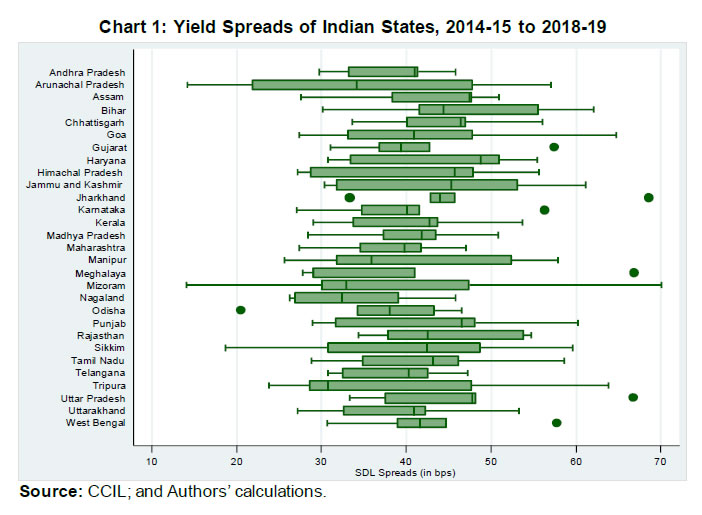

Further, the variations in the yield spread across time could be influenced by macroeconomic conditions and common risk factors while variations across states could only be attributed to state-specific perceived credit risk and liquidity. The average spread of SDL yields over central government securities of similar maturity showed significant variations across time. The data from 2005-06 onwards showed that the spread ranged from 90 basis points in 2009-10 to less than 10 basis points in 2014-15 (Chart 2).

II.3 Fiscal Performance of Indian States – Select Indicators

We discuss, in this section, the states’ fiscal performance in terms of various indicators that might impact the yield spreads. Gross fiscal deficit (GFD), which determines the borrowing requirements of states, influences the supply of SDLs that may impact yield spreads. The consolidated position of all states reveals that during the sample period, they, on average, have been able to contain their fiscal deficit under the targeted 3 per cent level, set out in the respective Fiscal Responsibility Legislations, barring the year 2016-17 (Table 3). States took over the Ujwal Discom Assurance Yojana (UDAY) scheme on their budgets, which impacted their deficit ratios¹⁰ during 2016-17.

Notwithstanding the convergence towards the target of 3 per cent of Gross State Domestic Product (GSDP) at the consolidated level, we observe significant variation across states in the deficit ratios (Chart 3). From the perspective of relative fiscal performance, inter-state variation in GFD is a crucial dimension. The box plot suggests a significant amount of divergence in GFD amongst states as well as across time (Chart 3). For example, Andhra Pradesh continued to have a GFD ratio¹¹ of around 4 per cent during the sample period, except 6 per cent for one year. The fiscal balance of Mizoram, on the other hand, varied from a surplus of 2.7 per cent of GSDP to a deficit of 7.7 per cent during the sample period. Some states, viz., Gujarat, Karnataka, Maharashtra and Odisha were able to consistently maintain their GFD ratios below 3 per cent level while the GFD ratios of some other states such as Andhra Pradesh, Bihar, Kerala and Rajasthan exceeded the 3 per cent target.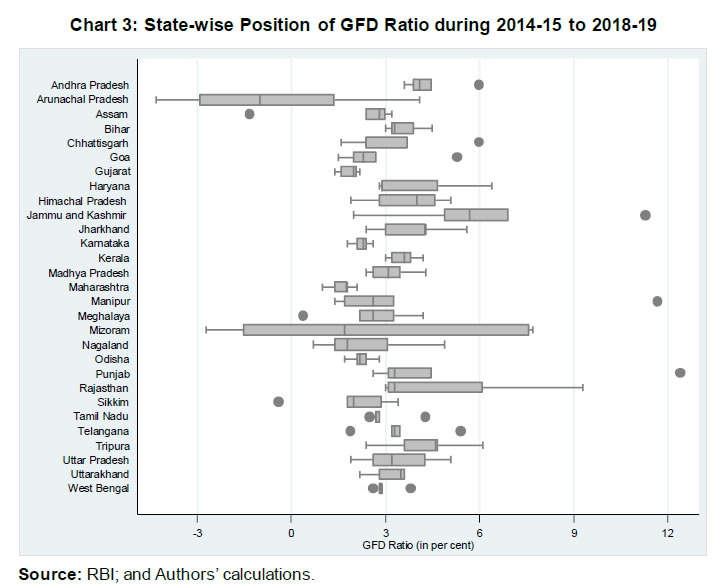

II.4 Financing the Deficit

Market borrowings have emerged as a major source for raising resources by states (Table 4). The other sources of financing include securities issued to National Small Savings Fund (NSSF), loans from financial institutions, provident funds, reserve funds, and deposits and advances. The decline in financing from NSSF securities reflects the decision of most states to opt-out from the operations of NSSF as per the recommendations of the Fourteenth Finance Commission (Union Budget, 2020-21).

The development of government securities market in the country has helped both the central and state governments to raise resources from the market. The share of market borrowings in financing the GFD of the central government started increasing since the beginning of the 1990s with migration from the administered interest rate regime to a market-oriented price discovery mechanism and introduction of a system of auctions for central government securities in 1992 (RBI, 2007). Market borrowings, which used to have a meagre share in financing GFD of state governments, emerged as the most important source of financing since 2007-08, partly due to a decline in the collections under NSSF.¹² The share of market borrowings in financing GFD of the states through market loans increased from below 20 per cent in 2006-07 to about 70 per cent in 2007-08 and continued around that level thereafter (Chart 4).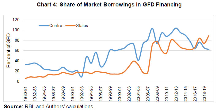

A comparison of market borrowings of centre and state governments since 2014-15 reveals that state governments’ market borrowings have grown at a much faster pace (Chart 5). Gross market borrowings of state governments increased almost three-fold over the sample period from ₹240 thousand crore in 2014-15 to ₹634 thousand crore in 2019-20. It may be worthwhile to mention that the state governments used to issue bonds up to 10-year maturity initially. However, with the development of the market for SDLs and a more active approach adopted by the states to manage maturity profiles of their debt, some of the state governments started issuing longer tenor securities since 2015-16. The Telangana government has issued the longest tenor security of 30 years maturity.

II.V Debt Position

Reflecting the cumulative impact of fiscal deficit, the overall debt of the states rose considerably during the first half of the 2000s, crossing 30 per cent of GSDP in 2003-04. Thereafter, the debt-GSDP ratio of states declined as several states followed a fiscal consolidation path stipulated under Fiscal Responsibility Legislations. The economic slowdown and the need for fiscal support again drove the debt levels upward after 2014-15. The increase in debt during 2015-16 and 2016-17 was partly attributed to loans and advances for power projects under UDAY, whereby states took over DISCOM debt. This has resulted in states’ outstanding liabilities increasing by 0.7 percentage points in 2016-17 (RBI, 2020). A comparison of debt-gross domestic product (GDP) ratio and debt-own revenue receipts ratio suggests that the latter declined to a lesser extent after 2005-06 indicating that the own revenue receipts did not match the pace of GDP (Chart 6a). Furthermore, the state-wise position shows that the debt-GSDP ratio, on average, ranged from a low of 16.1 per cent for Telangana to a high of 48.7 per cent for Jammu and Kashmir (Chart 6b).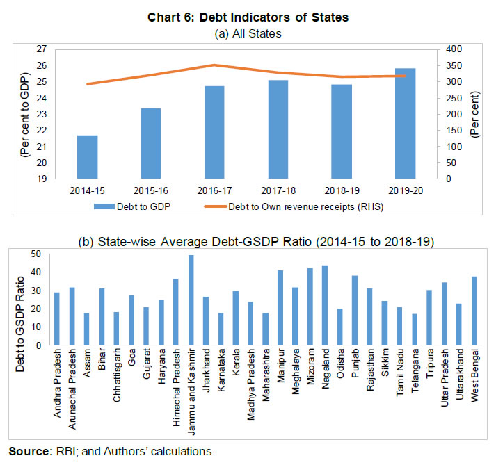

The expenditure pattern at the sub-national level in India indicates that the revenue expenditure constitutes about 83 per cent of total expenditure (Table 5). Slightly more than 50 per cent of expenditure was incurred on developmental activities such as social and economic services. States spend about 25 per cent of total expenditure towards committed expenditure including interest payments. The share of capital outlay, which can help in improving growth prospects through building requisite infrastructure by states was consistently below 15 per cent.

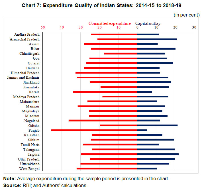A state-wise analysis shows significant variation in expenditure composition across states. It is evident from Chart 7 that the quality of expenditure seems to be predominantly determined by committed expenditure. The high committed expenditure, particularly on interest payments, has a tendency of a vicious cycle whereby lesser resources could be made available for productive expenditure, which in turn could adversely affect GSDP growth and revenue mobilisation. Investors could have a low preference for states with high committed expenditure and may demand higher yield spreads.

II.7 Revenue Generation Efforts

The ratio of debt to revenue is considered a key indicator of the fiscal prudence of a government. Revenue receipts of states in India could broadly be divided into two - transfer from the centre and own revenue. From the perspective of debt sustainability, revenue should include only their own revenues and untied transfers (Giugale et al., 2000). Own revenue of states in India consists of both tax and non-tax revenues which together constitute more than 50 per cent of total revenue receipts. On average, about 45 per cent of revenues came from states’ own tax collections while their own non-tax collections constituted about 8 per cent of revenues (Table 6).

There is significant variation across states in the share of own revenues in total revenue receipts with less industrialised and smaller states depending more on transfers from the central government. While the share of own revenues is generally lower in respect of north-eastern states, it varies significantly even for others. For instance, Haryana raised about 78 per cent of revenues from its own resources during the period 2014-15 to 2019-20, while the share was about 27 per cent in respect of Bihar (Chart 8).

III. States’ Performance Composite Index

The yield spread on subnational borrowings should be impacted by the fiscal performance of states (Beck et al., 2017; Sola & Palomba, 2015) as well as market micro-structure, such as trading mechanisms, price formation, depth and liquidity (Bhattacharyya et al., 2009; Bellas et al., 2010). Investors find it difficult to assess multiple factors and to analyse various risks while making their investment decisions. The combined effect of these factors eventually adversely affects the price discovery mechanism of subnational government securities. Therefore, we propose a composite index that can measure both – states’ fiscal performance and market development. The fiscal performance of a state is generally assessed in terms of various individual indicators such as deficit, debt, expenditure composition and revenue efforts. Similarly, market development¹³ could be assessed in terms of bid-cover ratio, turnover, liquidity, etc. The proposed composite index provides a single measure of states’ overall performance by integrating select indicators from each dimension.

III.1 Methodology

We consider 13 indicators, reflecting various aspects of fiscal performance, and combine them into five major sub-indices, viz., deficit index, own revenue effort index, expenditure quality, debt sustainability and market liquidity. These five sub-indices are then combined to form a composite index. Chart 9 illustrates the basic framework for the proposed index for the states’ performance.

We first construct the individual sub-indices and then combine these sub-indices to obtain the composite index. Each sub-index contains different dimensions/ indicators which are discussed below.

a) Deficit Index: It consists of the following two indicators:

(i) Revenue deficit (RD) as a proportion of GSDP at current market prices (RD/GSDP). Revenue deficit is defined as the excess of revenue expenditure over revenue receipts in a given year.

(ii) Gross fiscal deficit as a proportion of GSDP at current market prices (GFD/GSDP). Gross fiscal deficit is defined as the excess of total expenditure over non-debt receipts.

The negative value indicates a surplus and a positive value indicates a deficit. Following the practice, we express both the indicators¹⁴ as per cent of GSDP. A high revenue deficit is often associated with lower capital expenditure and higher current expenditure, which is often considered unproductive. Furthermore, this unproductive expenditure financed through borrowed funds may lead to a further increase in current expenditure in the form of interest payments, thereby creating a vicious cycle. The fiscal deficit represents the net borrowing requirements of a state which determines the supply of securities. Apart from the current supply of issuances, fiscal deficit also represents an increase in debt and therefore the future supply of issuances. Therefore, a lower ratio would be desirable.

b) Own Revenue Effort Index: It is constructed by combining the following two indicators:

(i) Own tax collection as a proportion of revenue receipts (OTC/RR); and

(ii) Own non-tax collection as a proportion of revenue receipts (ONTC/RR).

These two indicators measure the revenue-raising efforts of a state and indicate the degree of fiscal autonomy. Higher own revenue provides more flexibility to a state in its expenditure decisions and may also help in containing its deficit. Therefore, states with higher ratios are considered to be better placed.

c) Expenditure Quality Index: This sub-index measures the quality of expenditure primarily representing expenditure composition in terms of productive and non-productive components. We consider the following three ratios for this sub-index:

(i) Committed expenditure to total expenditure ratio;

(ii) Capital expenditure to total expenditure ratio; and

(iii) Development expenditure to total expenditure ratio.

The states with higher committed expenditure are left with lesser resources for other productive allocations, and therefore, higher committed expenditure is viewed as detrimental to the states’ fiscal health. On the other hand, capital expenditure is often viewed as having a multiplier effect on economic growth and consequent fiscal benefits in terms of an increase in revenues. Similarly, development expenditure includes resources allocated for the social services sector and economic services. Development expenditure includes some of the revenue expenditure, which is also considered a productive expenditure. A higher proportion of capital and development expenditure in total expenditure suggests better resource allocation by state governments.

d) Debt Sustainability Index: This sub-index consists of the following four indicators:

(i) Outstanding debt as a proportion of GSDP (OD/GSDP);

(ii) Interest payments as a proportion of revenue receipts (IP/RR);

(iii) Market borrowings as a proportion of gross fiscal deficit (MB/GFD); and

(iv) Maturity profile of state government debt.

The debt to GSDP ratio (OD/GSDP) reflects the debt burden of a state which is often considered as a major indicator of fiscal health. Furthermore, a high level of debt also suggests higher interest expenditure in the future. For debt sustainability analysis, interest payments to revenue receipts (IP/RR) suggest the ability of a state to service its debt without putting pressure on borrowings or productive expenditure (Kaur et al., 2018). Both these indicators capture the debt profile and a higher ratio suggests weaker fiscal health.

We also include the financing pattern in the index through the MB/GFD ratio. From the perspective of yield spread, a higher share of market borrowings could mean more supply of securities and therefore higher spread. We, however, postulate that a state that manages its finances better would be able to raise more resources from the market in a cost-effective manner. Apart from imparting liquidity to securities, this will also engender confidence amongst investors about the fiscal health of the state. Therefore, a higher share of market borrowings in financing GFD could help to lower the yield spread. The maturity profile captures redemption pressure on states’ debt – higher maturity means lower redemption pressure in near future.

e) Market liquidity index: It is constructed with the following two indicators:

(i) Number of trading days in a year; and

(ii) Turnover ratio.

The number of trading days in a year is calculated from the data on trades executed and reported on NDS-OM. If any state government security is traded at least once on a given day, it is considered a trading day. Turnover ratio, defined as trading volume as a proportion of outstanding state government securities, is another frequently used measure of liquidity. Both these indicators are included to measure the market liquidity of SDLs – the higher the number of days and turnover ratio, the more liquid a state government debt is.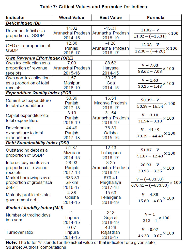

The indicators discussed above are characterised by large-scale variations that cannot be meaningfully combined by simple aggregation. We, therefore, first convert each indicator into an index following the methodology used to construct the Human Development Index (HDI) of UNDP (1990). For this purpose, we first identify the worst and the best value for each indicator for each year from 2014-15 to 2018-19 and transform the indicators into indices between 0 and 100 (Table 7). The worst and the best values¹⁵ are defined in such a way that all indices become unidirectional and could be horizontally combined to form the sub-indices, and finally the composite index. Thus, an increase in the value of an index would mean an improvement in fiscal performance and vice-versa.

It is evident from the above discussion that the proposed composite index represents the relative performance of a state compared to the best-performing state. Nevertheless, it can provide appropriate and effective guidance to state governments on the scope and direction of improvement. We have given equal weights to all the five sub-components while constructing the final composite index and all indices within each sub-index. One can argue that constructing an index based on observation of the worst and the best values of indicators may attach an implicit weight to the indicators (Dholakia, 2005). Moreover, if the weights remain constant spatially as well as temporally, it should not create a problem in comparability; and selection of a large number of indicators, instead of one or two, reduces the judgment error with regard to states’ performance.

III.2 The Index

We present the states’ performance composite index (SPCI) for the sample period in Chart 10 and Annex Table A2. The five sub-indices, which are used to prepare SPCI, are given in Annex Table A3. We observe large variations across sub-indices in a given state which strengthens the case for the construction of a single measure that can be used to assess states’ performance in fiscal management and market development. For instance, during 2017-18, for Punjab, the value of expenditure quality (EQ) was as low as 0.6, but the value of market liquidity (ML) was 72.4. Similarly, considerable variations were also seen across time with some states showing significant improvements in SPCI while others slipping on the ladder. The states like Karnataka and Gujarat have a relatively higher SPCI during the entire sample period while the states like Haryana and Telangana improved their SPCI significantly over the period from 2014-15 to 2018-19 (Chart 10).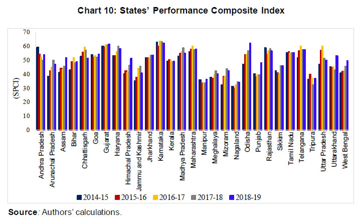

Analysis of sub-indices shows that some states like Rajasthan and Andhra Pradesh slid in ranking in 2014-15 mainly because of their own revenue generation. Northeastern states showed lower SPCI in the range of 29.7 to about 50 during the sample period. These states have a much lower value of market liquidity and own revenue indices. Kerala has an SPCI value of 46.7 during 2018-19 due to low performance in terms of both deficit management and own revenue generation. Telangana has the highest maturity profile index but has a below-average turnover ratio.

IV. States’ Performance vis-à-vis Yield Spreads

With the fiscal decentralisation in India, state governments migrated from the tap-based system to auction-based issuances of market borrowings since 2006-07. The issuances of sub-sovereign bonds, though dominant in some countries, have picked up in India recently. State government securities were valued using the yield to maturity method and investors used to add a uniform mark-up above the benchmark G-sec yield of equivalent maturity. However, RBI in its June 2018 policy decided that the securities issued by each state government should be market-linked, and hence, valued based on observed market prices (RBI, 2018a).

Sub-sovereign securities, generally, trade at a premium to sovereign securities. The difference in yields, referred to as yield spread, is an issue of debate across market analysts and academia. While one strand of literature supports that such yield spreads are attributed to fiscal performance of the states (Beck et al., 2017; Sola & Palomba, 2015), other studies, particularly in the Indian context, did not find many roles of fiscal performance (Bose et al., 2011; Saggar et al., 2017). It is rather attributed to typical market microstructure, such as trading mechanisms, price formation, depth and liquidity (Bhattacharyya et al., 2009; Bellas et al., 2010). Therefore, the composite index of states’ performance, constructed in the previous section incorporating both fiscal fundamentals and market microstructure could attract great importance in this line of research.

As discussed in the section on ‘Data and Stylised Facts’, the yields on SDLs in India carry a positive spread over the yields on central government securities with significant variation across states (Chart 1). We empirically examine if the yield spreads on SDLs in India can be explained by the SPCI, which incorporate fiscal indicators of a state – such as the fiscal deficit, revenue effort, expenditure quality, debt position, among others – as well as market liquidity of SDLs. Furthermore, the investor is more likely to make a decision based on last year’s performance as the relevant information for the current year would be available at the end of the year. Therefore, we hypothesise that states’ performance during the last year may impact the yield spread during the current year. Accordingly, we test the following hypothesis:

H₀: States’ performance doesn’t influence SDL yield spreads.

IV.1 Empirical model

To assess the impact of the SPCI on the yield spreads of state government bonds and to test the above hypothesis, we estimate the following model:

State-wise yield spreads are referred to as the difference between the yield on state government securities and yield on GoI securities of similar maturity. Our composite index takes into consideration a state’s overall performance with regard to fiscal and market-related indicators. Among the control variables, we consider real per capita income to control for the income impact on yield spreads, which may have implications on own revenue mobilisation of states. To control for the economic structure, we have considered the share of industry and share of services in GSDP composition. A state with more industrial/services share is expected to have a higher base for revenue mobilisation compared to a state with a lower industrial/services share. Bank credit and deposit are used to control for states’ financial position that may have implications on spread differentials. Financial variables are taken in a natural logarithm to have them on a similar scale.

Since the data on state fiscal indicators used in the construction of our composite index are available on annual basis, we use state-wise annual weighted average spreads, as published by CCIL, as our dependent variable. Furthermore, it was observed that there are some states which hardly borrow from the market (Chart 11). The states which are borrowing very low amounts from the market may distort the results, as the yield spreads of these states are more likely to be influenced by idiosyncratic factors, but will carry equal weights if included in the regression. Therefore, we treat such states (namely, Nagaland, Meghalaya, Tripura, Sikkim, Manipur, Arunachal Pradesh and Mizoram) separately in our empirical exercise.

IV.2 Empirical Results

IV.2.1 Descriptive Statistics

Year-wise and overall sample summary statistics of the yield spreads are presented in Table 8. The mean yield spreads, representing the average spread of state government securities over the GoI securities, is in the range of 29 bps for 2014-15 to 56 bps for 2018-19. Though the standard deviation of yield spreads was below 9 bps for many years, it was the highest at about 17 bps for 2016-17.

Furthermore, as observed from the interquartile range, interstate variation is in the range of 3-8 bps. Interestingly, after removing the states with minuscule borrowings, the mean spread increased until 2016-17, but decreased thereafter, possibly because of administered interest rates which might have helped states with minuscule borrowings to get lower rates. The distribution of yield spreads slightly shifted towards the right until 2016-17, and slightly to left thereafter suggesting market-determined interest rates.

To understand the yearly movement of the composite index (SPCI), we present summary statistics of the index for each year in Table 9. The mean index showed an improvement during the study period. We observe that the average performance of states which access the market for raising resources is better, as observed from the mean index. Unlike yield spreads, the index moved towards the right for all the years after making adjustments for states with minuscule borrowings. The interquartile range for states which borrow at least 0.2 per cent of total borrowings was smaller compared to all the states, suggesting an invisible competition among states with regard to their fiscal performance.

IV.2.2 Regression Results

The estimated results¹⁶ are presented in Table 10. First, we estimate the model including all the states in the sample. The results given in column (1) of Table 10 show that the composite index did not have any impact on the yield spreads. As discussed above, idiosyncratic factors in respect of the states with negligible market borrowings might have distorted the results.

We, therefore, estimate the model for only those states which have borrowed at least 0.2 per cent of the total borrowings by all the states during the sample period. For this, we force the index of states which have negligible borrowings to zero to save on the number of observations and degrees of freedom (column (2)). Further, we split our index variables into two groups: one takes index value for states with at least 0.2 per cent of total borrowings and the other with less than 0.2 per cent of market borrowings (column (3)). Finally, we augment the specification of column 3 with year dummies and results are given in column (4).

The results indicate that the index has a negative and statistically significant impact on the yield spreads of states. The sign and statistical significance of the coefficient remain broadly unchanged in different specifications suggesting the robustness of the results. It is evident from the index construction method that fiscal performance is the key aspect of the index¹⁷ and better fiscal performance yields a higher value of the index. The negative relationship of the index with the yield spread, thus, suggests that the states can reduce their cost of borrowing through improvements in fiscal management.

We analyse the impact of each sub-component of our composite index on the yield spread. For this purpose, we estimate the model including individual sub-components as explanatory variables rather than the composite index in different specifications and then including all the sub-components together (Table 11). We find that deficit and expenditure quality indices are both negatively related to yield spreads and are statistically significant at the 10 per cent level. It may be mentioned that the value of the index is higher when the deficit is lower, and when expenditure quality is better. The other two sub-components, own revenue effort and debt sustainability are not significant. The market liquidity is negative and significant at the 5 per cent level implying that the more liquid the SDL security, the lower the spread.

To further examine the robustness of the index, we estimate the regression with a truncated index including only 3 sub-indices (that were individually significant in the regression). It gives broadly similar results which further supports the robustness of the empirical findings (Annex Table A4). The statistical significance and the magnitude of the coefficients, however, suggest that the composite index (consisting of 5 sub-indices) has better explanatory power than the truncated index. This could be due to the interaction that may take place among different dimensions of state performance in fiscal management and market developments and might have strengthened the explanatory power of the overall composite index.

The results of the empirical exercise discussed above suggest that the fiscal performance indicators along with market liquidity have a significant impact on SDL yield spreads. The results are particularly important in view of the existing literature which suggests that the fiscal position of states does not influence their yield spreads. The findings of the paper have clear policy implications for states according to which the cost of borrowing of the states may be reduced by improving their fiscal performance. Analysis of individual components of the index provides further insights which are in line with the existing literature. The debt indicator individually turned out to be a statistically insignificant determinant of yield spread which is in line with RBI (2018b). The insignificant impact of the debt indicator on yield spreads could be attributed to the inertial nature of the debt, as this indicator is less likely to vary from year to year. Furthermore, investors may be looking for those fiscal variables which are more indicative of a forwarding outlook whereas the outstanding debt indicates more of the past fiscal performance of a state. Similarly, the own revenue mobilisation effort indicator is also not statistically significant, which is counter-intuitive. This could, however, be reflective of the fact that states may not have much flexibility in raising their revenues. Also, revenue-raising efforts give a perception that the concerned state levying more taxes may be detrimental to investment and long-term growth prospects.

The deficit indicator turns out to be a significant variable to influence yield spreads which are in line with the expected sign. The higher deficit could affect yield spread through the supply channel as well as through adverse impact on future outlook, via increased debt and interest payments. Expenditure quality also showed a negative and significant influence on yield spread. Better quality of expenditure, which reflects a higher share of capital and productive expenditure, would lead to increased investment and improve the long-term growth prospects of a state. The positive impact (in terms of lower spread) of better growth prospects of a state on its yield spread may emanate from investors’ perception of better revenue outlook, lower deficit and supply of bonds in the future. More importantly, the results suggest that the overall composite index consisting of five sub-indices is a better indicator of states’ performance in fiscal management and market developments as compared with the truncated index with a lesser number of dimensions.

The results provide a menu of choice to states for their fiscal policy. They can reduce their cost of borrowing by reducing their fiscal deficit and/or by improving their quality of expenditure. Efforts to raise their own revenues may not yield much in terms of reducing their cost of borrowing. Another major finding of the paper relates to the market liquidity of SDLs which has a significant impact on yield spread. This has clear policy implications for the debt management strategy of states whereby they can reduce their cost of borrowing by improving liquidity through the re-issuance of SDLs and other measures.

Coming to the relevance of the paper for investors and price discovery, the findings provide useful information that can enable investors to price SDLs in a more informed manner. Specifically, the composite index provides a single barometer that can be used by investors to make their SDL investment decisions. The assessment of the fiscal position of a state could remain rather obscured in the absence of a single measure, and this could have undermined the price discovery mechanism. The extant literature emphasises that investors incorporate states’ fiscal performance while pricing the SDLs (RBI, 2018b) but the absence of a unique metric to assess the states’ performance leaves investors puzzled. Thus, the composite index developed in the paper will fill this gap and make the price discovery of SDLs more efficient.

V. Conclusion and Policy Implications

A significant increase in market borrowings of state governments over time has subjected the fiscal authorities to the need for greater scrutiny by investors. The moot question is whether states’ fiscal performance matters for SDL yield spreads. The narrowly clustered SDL spreads, in a majority of auctions, make this question more pertinent. Moreover, the existing empirical literature in the Indian context finds a weak association between SDL yield spreads and fiscal metrics, suggesting the lack of perceived risk by investors across Indian states in the market borrowings space.

We, therefore, postulated in this paper that there is perhaps a need for arriving at a better and holistic measure of fiscal performance including the market-related information to explain the SDL yield spreads. We constructed a states’ performance composite index (SPCI) - incorporating fiscal, debt and market-related indicators and examined whether fiscal metrics captured in the index have any impact on SDL yield spreads. We found a statistically significant association of the index with spreads suggesting that better fiscal management and improved market liquidity can help states to reduce their cost of borrowing. Analysis of individual sub-indices revealed that deficit, expenditure quality and market liquidity are the important factors in determining yield spreads.

The findings of the paper have important policy implications. The composite index can be used by both – state governments and investors – for assessing states’ fiscal performance. State governments can use the index to orient or reorient their fiscal policies towards improving their performance in order to reduce the cost of borrowing. Analysis of individual sub-indices provides a menu of choice to state governments. For example, a state can offset the adverse impact of a high fiscal deficit by improving its expenditure quality. A state can also reduce its cost of borrowing through the re-issuance of SDLs (that will improve its liquidity). From the perspective of price discovery, it is often felt that investors find it difficult to assess the states’ performance as multiple indicators often show diverging assessments. Thus, the composite index developed in the paper provides investors with a single measure to make more informed investment decisions, thereby making the price discovery mechanism of SDLs more efficient.

^@ Ramesh Jangili (rjangili@rbi.org.in) is Assistant Adviser in Department of Statistics and Information Management, Hyderabad; N.R.V.V.M.K. Rajendra Kumar (rajendrakumar@rbi.org.in) is Chief General Manager in Internal Debt Management Department; and Jai Chander (jaichander@rbi.org.in) is Director in Department of Economic and Policy Research, Reserve Bank of India.

^* Useful comments from Dr. Seema Saggar, Dr. G P Samanta, Shri Rahul Agarwal, an anonymous external referee and other participants in the DEPR Study Circle are gratefully acknowledged.

¹ In this case, the issuers are the Indian state governments.

² We have presented the gist of recent studies on the relationship between states’ performance and cost of borrowing in Annex (Table A1).

³ G-sec market in India is more liquid around the 10-year maturity bucket. SDLs issued by state governments in a 10-year maturity bucket should also enjoy a similar liquidity premium when compared to other maturities.

⁴ Yield spread refers to the difference between the yields on State government securities with that of GoI dated securities of similar maturity. For our empirical analysis, the SDL yield spread is arrived at by taking the weighted average of spreads during the year, weights being the amount borrowed with that specific spread. For more details on SDL yield spreads and the way they have been arrived at, kindly refer to the CCIL’s publications on SDL yield spreads, which are available at https://www.ccilindia.com/Pages/default.aspx.

⁵ Perceived risk is an important aspect of debt markets that may not be eliminated completely as suggested by some anecdotal evidence in the case of Indian states. Perception of risk of sub-national government bonds could vary due to different factors such as institutional arrangements, inter-government transfers, and tax revenue sharing mechanism. For instance, sub-national governments receiving more transfers from the central government were found to pay the lower cost of borrowing in Germany, Spain and Canada (Sola & Palomba, 2015).

⁶ Illustratively, there were four auctions during February 2021 (on Feb 2, Feb 9, Feb 16 and Feb 23). The observed interstate spread for 10-year bonds was 14bps (6.99-6.85), 11bps (7.05-6.94), 15bps (7.08-6.93) and 17bps (7.24-7.07), respectively, during these four auctions. If one would look at the simple average of these spreads, it worked out to be 14.25 bps. However, it needs to be noted that the minimum cut-off yield during February 2021 was 6.85 per cent and the maximum cut-off yield was 7.24 per cent, resulting in a spread of 39 bps. When one considers it for the entire year, the spread may be even higher.

⁷ On March 23, 2020 auction day, the cut-off yield for Telangana with 10 years maturity was 7.99 per cent, whereas, the cut-off yield for Gujarat, Rajasthan and Uttarakhand with similar maturity was only 7.45 per cent, resulting in an inter-state spread of 54 basis points. It is difficult to take this as an outlier, as the second-highest cut-off yield of 7.93 per cent is observed for Uttar Pradesh with similar maturity resulting in an inter-state spread of 48 basis points if we eliminate/discard Telangana in that auction (https://www.rbi.org.in/Scripts/BS_PressReleaseDisplay.aspx?prid=49557).

⁸ The State of Jammu and Kashmir was reorganized as ‘Union territory of Ladakh’ and ‘Union territory of Jammu and Kashmir’ vide The Gazette of India dated 9th August, 2019 (The Jammu And Kashmir Reorganisation Act, 2019), however, Jammu & Kashmir in this study represents the united Jammu and Kashmir state before the reorganization, as the study period is upto March 2019.

⁹ The box plot shows the minimum, lower quartile, median, upper quartile, and the maximum values of a variable along with outliers as dots.

¹⁰ The impact of UDAY was estimated to be 0.7 per cent of GSDP during 2016-17.

¹¹ GFD ratio is defined as GFD as a percentage of GDP/GSDP.

¹² During 2007-08, the Government of India provided an additional allocation of ₹35,780 crore to states on account of shortfall in collections under the NSSF. Incidentally, all the state governments have been raising market loans through the auction route since 2006-07 and greater transparency has been brought in the market borrowing programme of state governments.

¹³ The liquidity of SDLs is concentrated around a few securities and the turnover ratio of SDLs is significantly lower than that for GoI securities. However, the SDL market is gaining momentum and all states are on the same footing, therefore, all states are expected to reap the benefits from market development.

¹⁴ Though both the indicators represent deficit management, these two indicators have different implications. For instance, a state can have a revenue surplus but run a fiscal deficit to incur higher capital expenditure. This would give a superior fiscal outcome as compared with a revenue deficit induced fiscal deficit.

¹⁵ The worst and the best values of indicators are observed values based on the data during the sample period. These values may change when we include more years, however, the ordering of the states will remain unchanged unless a state makes improvement in relation to other states.

¹⁶ The results presented are from fixed effects (FE) specification. One can argue that random effects (RE) specification can also be tried. However, the FE estimator is almost always much more convincing than the RE estimator (Wooldridge, 2010). Further, the Hausman (1978) test, which is used to decide between FE and RE models, confirmed the selection of the FE model.

¹⁷ Though we have five broad categories in the composite index, fiscal performance is the key aspect covering deficit management, revenue efforts and expenditure quality.

References

Beck, R., Ferrucci, G., Hantzsche, A., & Rau-Göhring, M. (2017). Determinants of sub-sovereign bond yield spreads - The role of fiscal fundamentals and federal bailout expectations. Journal of International Money and Finance, 79, 72-98. https://doi.org/10.1016/j.jimonfin.2017.08.003

Bellas, D., Papaioannou, M. G., & Petrova, I. (2010). Determinants of emerging market sovereign bond spreads: Fundamentals vs financial stress. IMF Working Paper, No. 10/281. International Monetary Fund.

Bellot, N. J., Selva, M. M., & Menéndez, L. G. (2017). Spreads of bonds issued by sub-sovereign European governments. Journal of Innovation & Knowledge, 2(3), 146-154. https://doi.org/10.1016/j.jik.2016.10.002

Bhattacharyya, I., Roy, M., Joshi, H., & Patra, M. D. (2009). Money market microstructure and monetary policy: the Indian experience. Macroeconomics and Finance in Emerging Market Economies, 2(1), 59-77. https://doi.org/10.1080/17520840902726326

Bose, D., Jain, R., & Lakshmanan, L. (2011). Determinants of primary yield spreads of states in India: An econometric analysis. RBI Working Paper, No. 10/2011, Reserve Bank of India.

Diamond, J. (1989). Government expenditure and economic growth: An empirical investigation. IMF Working Paper, No. 89/45. International Monetary Fund. https://doi.org/10.5089/9781451974157.001

Dholakia, A. (2005). Measuring fiscal performance of states: An alternative approach. Economic and Political Weekly, 40(31), 3421-3428. https://www.jstor.org/stable/4416963

Edwards, S. (1984). LDC foreign borrowing and default risk: An empirical investigation, 1976-80. The American Economic Review, 74(4), 726-734. https://www.jstor.org/stable/1805136

Giugale, M., Trillo, F. H., & Oliveira, J. C. (2000). Subnational borrowing and debt management. Achievements and Challenges of Fiscal Decentralization: Lessons from Mexico, 237-270.

Hausman, J. A. (1978). Specification tests in econometrics. Econometrica, 46(6), 1251-71. https://doi.org/10.2307/1913827

Kanungo, B. P. (2018). State government market borrowings – issues and prospects. RBI Bulletin, September, Reserve Bank of India.

Kaur, B., Mukherjee, A., & Ekka, A. P. (2018). Debt sustainability of states in India: An assessment. Indian Economic Review, 53(1-2), 93-129. https://doi.org/10.1007/s41775-018-0018-y

Nath, G. C., Pawaskar, V. & Shiraly, P. (2019). Microstructure of sub-sovereign bond spreads – The case of federal state bonds in India. The Clearing Corporation of India Ltd. Working Paper, November.

Pattnaik R.K, Bose D., Bhattacharyya, I., and Chander, J. (2005). Public expenditure and emerging fiscal policy scenario in India. Public Finance, Banca d’Italia, Italy.

RBI (2007). Report on Currency and Finance, May 31, Reserve Bank of India

RBI (2018a). Statement on developmental and regulatory policies, June 06, Reserve Bank of India

RBI (2018b). SDL yield spreads: Do they reflect underlying fundamentals? in State Finances: A Study of Budgets, Box III.2, Reserve Bank of India, 35-37.

RBI (2020). State finances: A study of budgets, October 27 and earlier reports, Reserve Bank of India.

Saggar, S., Rahul, T. & Adki, M. (2017). State government yield spreads – Do fiscal metrics matter?, RBI Mint Street Memo, No. 08/2017, Reserve Bank of India.

Sola, M. S., & Palomba, M. G. (2015). Sub-national government’s risk premia: Does fiscal performance matter?, IMF Working Paper, No. 15/117, International Monetary Fund.

Tanzi, V. and Zee, H.H. (1997). Fiscal policy and long-run growth. IMF Economic Review, 44, 179–209. https://doi.org/10.2307/3867542

United Nations Development Programme (UNDP) (1990). Human Development Report 1990- Concept and Measurement of Human Development, New York.

Wooldridge, Jeffrey M. (2010). Econometric analysis of cross section and panel data (Cambridge: MIT Press).

Annex