Press Release RBI Working Paper Series No. 13 Is Implied Volatility Index (VIX) a Forward-Looking Indicator of Stock Market Movements in India? Amarendra Acharya, Subrat Kumar Seet and Prakash A. Salvi@ Abstract 1 The paper analyses the relationship between the implied volatility index and stock index in the Indian context over a relatively long period and explores whether the former can act as a forward-looking indicator for stock market investments. The findings suggest that a positive return on the stock index decreases the implied volatility, while a negative return increases it. Also, negative returns on the stock index generate larger changes in implied volatility as compared to positive returns. The size of the return too plays a major role in influencing the change in the implied volatility index. A higher level of volatility is seen to influence the buying decisions of the traders, particularly for investments at a duration of 20- and 60-days, as is the case with the stock markets in the US. JEL Classification: D53, G11, G41 Keywords: Implied Volatility Index, Forward-looking return, OLS Newey-West Introduction Financial market turbulence has often battered the global financial system. On many such occasions, governments across the globe have been forced to adopt measures to contain the economic fallout arising from the fragility of the financial markets. Such occasions have also underlined the need to find measures that can provide better insights into the behaviour of the financial markets. In stock markets, funds are raised from the investors for investment, and in exchange, the investors get a share in the profit of the firm. However, these investors face considerable uncertainty from the erratic movements in the market. Such uncertainty in the future returns is quantified through a volatility index. The Chicago Board Options Exchange (CBOE) first created a volatility index for the stock market, namely, the VIX. It acts as a barometer for expectations of volatility for the ensuing 30 days. In the Asian-Australian region, India started using it for the first time with its stock exchange disseminating an implied volatility index (Kumar, 2012). The implied volatility index is a measure of volatility perceived by market participants over a shorter horizon in the future. It is considered as the measure of the risk in the stock market. This index is an indicator of the anticipated fluctuation of the market and is generated on the basis of the order book of the underlying index options (NSE India). It is keenly watched by market participants and researchers to get a sense of the future behaviour of the market. The index generally reproduces the mean diversion of the fluctuation of a value around the long-term variance. It is also known as ‘fear gauge’ (Whale, 2009). The level of volatility is dependent on the level of price swings. A higher volatility value of the index indicates more swings in the price of the underlying stocks. A low level indicates that investors do not foresee much uncertainty in the market. While a high level implies turbulence in the financial markets, the sources of such volatility can be different. The literature suggests that volatility in financial markets is generated from longer trading hours, and the frequent arrival of new information both anticipated and unanticipated (Ross, 1989), and also by the positions taken by participants in the market and their unwinding (Brandt and Kavajecz, 2004). Another source of volatility can be the changing sentiments of investors (De Long et al., 1990). The behaviour of the implied volatility index is closely tracked by all stakeholders in the financial markets. There is a belief globally that a rise in volatility in the market generally brings with it a sharp fall in the stock index. There are two theories that explain this negative relationship between the stock index return and changes in the implied volatility index. Black (1976) postulated the leverage hypothesis which states that negative shocks to return increase financial leverage, making the stocks riskier and in turn increasing the volatility. Similarly, Poterba and Summers (1986) conceptualised the feedback hypothesis which highlights that any innovations to volatility (mostly positive ones) lower the returns. If expected future stock returns increase with an increase in volatility, as an after effect the current stock prices are likely to fall to adjust to this change in future expectations. It relies on the existence of time-varying risk premiums that link the changes in volatility and returns. There are multiple studies on the asymmetric relationship between volatility and stock return (Schewart, 1989, and Flemming et al., 1995). Studies on the Indian stock market too highlight the negative relationship between the stock index return with the relative change in the India VIX, and the two indicators tend to move independently of each other at the time of high upward movements in the market (Kumar 2010, Thenmozhi and Chandra, 2013). Interestingly, in the recent past, there have been episodes when sharp increases in equity prices have been associated with increases in implied volatility, indicating that the investors expected a greater volatility in the equity prices even in a rising market. These episodes of unidirectional movements have once again thrown open the research question concerning the relationship between market volatility and financial asset prices. Some market participants have highlighted that the India VIX going above 20 does not necessarily mean negative returns for the markets in the near term2. While a rise in the VIX generally brings market corrections, it is not necessarily deterministic3. There is a belief that markets are efficient, and hence cannot be predicted on the basis of implied volatility (Giot 2003). Finally, there are some market participants who believe that the implied volatility index is an indicator for buying /selling in the market. To address this emerging research question, Giot (2003) studied if high levels of VIX in the US market can be an indicator of the bottoming out of the market, and whether in this condition investors can go for fresh purchases expecting a rise in the market subsequently. His result indicated that extremely high levels of VIX acted as good buying points, and very low levels of VIX signalled good selling points. The present paper attempts to examine the various facets of the relationship between the stock index return and the change in implied volatility index in the Indian context and compares this relationship with those in the markets of the advanced economies (AEs), particularly the US. There is a view that empirical work on this relationship has become challenging with the changes in the prediction horizon, stock index, and data period (Ederington and Guan, 2010). The increasing global integration of the Indian stock market and the widening of its participants’ base have further added to the challenges. The scope of this paper is much broader than the earlier ones, as it looks for statistical clues in the market when the stock market and the volatility index move in the same direction. This paper also examines to what extent the volatility level can be used as a signal for purchases/sells in the Indian stock market at different time horizons, particularly by assigning ranks to the volatility levels of all days. While there have been studies comparing the Chinese and German markets with that of the US, there has been limited work comparing the Indian market with the US. The paper uses the framework adopted by Giot (2003). The hypothesis is that the behaviour of the stock market in India will be different from that in the US, as the US stock market is the cynosure of global investors and where the best companies in the world operate. Also, the US allows for a free flow of capital. The paper is structured as follows: Section II highlights the origin and calculation of the CBOE VIX and India VIX (IndVIX); Section III reviews the literature; Section IV describes the movements in S&P 500 and CBOE VIX as well as Nifty 50 and IndVIX during 2009 to 2020; Section V analyses the empirical relationship between the stock index and the volatility index, and the concluding perspectives are given in the last section. II. The Origin and Evolution of VIX The construction of the volatility index (VIX) has been discussed in a white paper released by CBOE VIX (Formula of VIX is given in Appendix A.1), and it is reproduced below: The VIX, operated by the Chicago Board Options Exchange (CBOE) from 1993, was designed to capture the expected fluctuation in the market. In the stock market, the stock index is constructed with the use of the prices of the shares constituting it. But the VIX is calculated from the weighted prices of call/ put options over many strike prices. The prices are mid-points of option bid/ask price quotations. The calculation of this index follows certain pre-fixed criteria in the selection of the options. The CBOE collaborated with Goldman Sachs in 2003, and made a modification in VIX, and this modified measure is being utilised by market participants to track expected volatility. It is derived by taking the strike prices of options of the S&P 500 index. With a well-defined formula behind it, this index emerged as a widely accepted tool regarding volatility trading/ hedging. In 2004, the VIX futures contract started operating in the same exchange. Then in 2006, the VIX option contract was launched that became a highly successful product. A well-developed market now exists for trading in VIX-related products. Over time, the CBOE has developed several other volatility indices, i.e., CBOE Nasdaq-100 volatility index, CBOE DJIA volatility index, CBOE Russell 2000 volatility index, and CBOE S&P 500 three-month volatility index. The VIX methodology has been refined to create a volatility index for commodities and currencies, such as the CBOE Crude Oil Volatility Index, CBOE Gold volatility index, CBOE Euro-Currency volatility index, etc. In fact, the opposite movements of volatility and stock market indices imply the benefit that can be derived from diversification and by investment in volatility-related products available in the market. This index has been extensively used for research, as the information relating to it is available for more than 20 years in the case of the US. The comprehensive information has been useful to study the movement of the share prices in the changing market conditions. It quantifies the perceived volatility in the stock market of the US. It is derived from the near- and next-term call/put options, generally belonging to the first and second contract months. Near-term options are taken when there are at least seven days to expiration. The reason is to avoid the anomalies arising out of the movements in prices close to expiration. Once the expiration is less than seven days, the calculation is done by taking the contracts of the second and third months. The out-of-the-money SPX Call/Put options on both sides of an at-the-money strike price are used in the computation of VIX, taking options having non-zero bid prices. With a rise in volatility, the range of the strike prices of the options also expands. And with a fall in volatility, the boundary of the strike prices also contracts. VIX contains all the information regarding the average of quoted bid and ask prices of all selected options. It can be seen from the formula that the price of every selected option directly affects the VIX values. In India, the India VIX (IndVIX4) was launched by the National Stock Exchange (NSE) in 2008, computed on the basis of the NIFTY index options prices. III. Literature Review There is extensive literature on the general behaviour of volatility indices, and their relationship with the stock returns. At the international level, there are studies (Schwert 1989, and Flemming et al., 1995) that highlight that the implied volatility index has a negative and asymmetric association with the stock market return. The negative stock market movement is associated with larger absolute changes in the volatility index than positive stock market movement. Giot (2003) further confirms this for the S&P100 index and adds that the VIX is more sensitive to negative returns in the low-volatility period, indicating investors’ response to be aggressive to negative returns, particularly in a less volatile phase. But the response is weak in a high volatile phase. With regard to its predictive capacity, it has a strong relationship with the future realised volatility though it is not free from biases. This property indicates that this index can act as a useful indicator for perceived stock market volatility, compared to the first-order autoregressive volatility model. Further, the VIX acts as a signaling mechanism for bottoming out of the market and indicates oversold conditions. Hence, positive forward-looking returns are expected from long positions triggered by extremely high levels of implied volatility. Thielen (2016) replicated the Giot (2003) study for Germany and compared the empirical findings with that in the US. It used the VIX as a proxy for volatility, and the returns of the stock indices of the S&P 500 and the DAX. The daily change in the VIX did not predict either negative or positive stock market return and hence the paper did not support the view that a change in the VIX affected stock market returns. Indirectly, the paper contradicted the finding of Giot (2003) and highlighted that the rate of change in the VIX is not a useful tool for investors to directly use it as a signal for trading. Another study along similar lines by Chengli and Yinhong (2016) compared the relationship between the two in the Chinese stock market with the US market. The regression between the implied volatility index and the underlying stock index, and also through a lag of these, showed a negative and asymmetric relationship between implied volatility index change and the return in the stock index in the US market. The CBOE VIX index was seen to be forward-looking. In the US market, the relationship was negative in general, but in China, the relationship was negative for some period. The study highlighted that the relationship was not statistically significant in the case of the Chinese market. The Chinese VIX index did not appear to be forward-looking. Hibbert et al. (2008) offered a behavioural explanation for the asymmetric return-volatility relation, by examining the short-term dynamic relation between the S&P 500 index return and changes in the volatility index with the use of daily and intra-day level data, while the past studies had used data with weekly or monthly frequency. The paper added to the literature by linking the behavioural characteristics of the traders with the results. The behavioural characteristics are representativeness, “affect”, and extrapolation bias. The representativeness signifies that larger negative returns and larger volatility are characteristics of market behaviour. The “affect” characteristic suggests that people form emotional associations with activities, where a positive “affect” appears good while a negative one comes as bad. The extrapolation bias indicates investors anticipate volatility increases to continue temporarily into the future. The same paper ascribed the relation between the stock index and volatility index to neither the leverage hypothesis nor the volatility feedback hypothesis, but to the behavioural characteristics. The leverage hypothesis suggests that the primary relation should exist from returns to volatility over a long period, not contemporaneously. Since lagged returns are not significant, the leverage explanation is not a robust one. The significance of the effect of lagged volatility changes supports the behavioural extrapolation bias. Banerjee, Doran, and Peterson (2006) extended the prior work of Giot (2003) and found that implied volatilities predict the security return which, in turn, points to the likely inefficiency of the market. The relationship was seen to be stronger for high beta stocks in S&P 500. Also, it was stronger for 60-day returns than for 30-day returns. There have also been some studies on the other properties of CBOE VIX that indicate that the VIX shows virtually no evidence of seasonality. There is a slight intra-day decline in the volatility index while no seasonality is observed in the intra-week data. Its daily changes have autocorrelation in them. Mean reversion is noted in the weekly data of this index. There is some literature on the general behaviour of the implied volatility index in India. Kumar (2010 and 2012) and Shaikh and Padhi (2016) studied the volatility index launched in India in 2008 and found that the stock market return and change in the volatility index are significantly negatively related and that too only in one direction, specifically during the descent of the market. A different type of finding was also reported in other studies. The negative and positive return shocks have opposite impacts on market volatility, and further, negative return shocks bring in significant changes in the level of implied volatility than positive return shocks. The returns on the two indices move independently at the time of high upward movements in the market (Thenmozhi and Chandra, 2013). When the market witnesses a downturn, the relationship is not much significant for higher quantiles. The application of quantile regression also showed that Indian VIX change was negatively related to stock market returns (Kumar, 2010). The result confirmed that the causality runs from a stock return to changes in volatility index, but not the other way. Investigation showed the presence of seasonality in the data, and also a Monday effect was found to be significant. These findings are similar to Flemming et al. (1995) for the US market. The empirical exercise in Kumar (2010) was attempted using data for a very short period, and hence, its findings need to be verified against data for a longer period. Further, India VIX is found to be a better measure of volatility than traditional measures, such as ARCH/GARCH models. It is also better than realised volatility estimates such as the standard deviation of historical returns, the daily variance estimates, and the monthly sum of stock returns. Bagchi (2012) studied the direct and cross-sectional relationship of India VIX with the stock return in relation to three parameters that are important aspects of behavioural finance: stock beta, market-to-book value, and market capitalisation. It examined the relationship after constructing six portfolios on the basis of the above-mentioned three parameters by dividing the data into two distinct parts, i.e., lower percentile and upper percentile, and then computing their returns for 30-day and 45-day holding periods. The results confirmed through multiple regression analysis that VIX has a positive and significant relationship with the returns of the above six portfolios. The relationship was found to be larger for a 45-day holding period return as compared to a 30-day holding period return. However, the biggest deficiency of the study was that it was carried out over a very short period, hence the result could be biased. A longer time period is needed to remove the bias. Further, there have been different levels of impact depending on the size of the positive and negative return shocks (Shaikh and Padhi, 2016). While VIX rises on the day of the opening of the market it falls on the day of the option expiration, and these findings create ground that it can be used for making profits by trading in VIX futures/options. Shaikh (2018) examined the relationship between the Indian volatility index and stock returns in the securities market, based on data from 2009 to 2015, and the results confirmed that there is a negative correlation between them, which is more prominent when the VIX is higher. There is also an asymmetric relationship between India VIX and stock returns and the magnitude of asymmetry is not identical; and hence, VIX is more of a gauge of investors’ fear and portfolio insurance price. The impact of changes in the stock return on India VIX is greater when there are negative returns as compared to positive returns. In the case of Nifty and S&P 100, there is no significant relationship discernible except for one period lag; and this finding is inconsistent with the hypothesis of contemporaneous asymmetry. The Indian VIX exhibits certain characteristics like volatility persistence, mean reversion, and a negative relationship with stock market movements, but has a positive association with trading volume. Further, overnight volatility movements from the US market have a significant effect on the Indian stock market volatility, but transmission from the Indian stock market to the US market is not seen. However, the stock market volatility in Japan seems to neither influence volatility in the Indian stock market nor it gets influenced by the movements in the Indian stock market. A rise in the US VIX increases the Indian volatility index, a result that brings out the implications for the portfolio diversification, volatility traders, and options trading-time in the equity markets (Kumar, 2010). Yeh and Tseng (2007) is another attempt in the direction of understanding the asymmetric relationship between return and volatility. The asymmetric effect is explained as a natural result from leverage, and also due to the feedback effect from expected volatility. Among the other studies, Chiang (2012) applied the bivariate GARCH model with TAR to examine the level of transmission between volatility and return using data on S&P (NASDAQ) and VIX (VXN) since the introduction of VIX (VXN). Additionally, only the lagged negative return has a bidirectional causal effect in the low-fear regime for the S&P 500/ VIX series. The VIX index has a stronger pricing effect on S&P 500. But there is no obvious lead-lag relationship between NASDAQ and VIXN index. The return and volatility responses to high-fear and low-fear episodes are asymmetrical. From the review of the empirical literature, it is clear that most studies for India have been conducted over a shorter time period. There are studies which juxtapose the relationship between stock return and implied volatility index in a particular country with that of the US. However, there is limited work comparing the relationship between India with that of the US. The present paper addresses this gap with (a) the use of data over a longer time period; (b) examining situations where the size of return influences the relationship between the two indices; and (c) comparing the Indian case with that of the US. IV. Movement of Stock Indices and Volatility Indices In the past decade, stock markets across the globe have responded to global as well as domestic factors, and the implied volatility indices also moved in conjunction with the stock indices. The volatility index reflects the anticipated volatility of the stock market over the coming month. A larger value of the index indicates higher prices for options, indirectly highlighting uneasiness among investors. A lower index indicates lower prices for options, highlighting a stable and smooth market in the near future. Chart 1 presents the movements in the US stock market and CBOE VIX during 2007-2020. The left axis gives the closing of the S&P 500 while the right axis gives the US VIX. The biggest spike in the US volatility index occurring during the global financial crisis (GFC) of 2008 coincided with the biggest fall in the stock market. Then it spiked again in 2011 during the European sovereign debt episode and in August 2015 as the stock market in China plunged. In India, the high VIX was witnessed around the time of the global financial crisis, followed by the jump during the taper tantrum episode of 2013 and then during the general election of 2014. Recently, the VIX reached a high with the onset of COVID-19 (Chart 2). On most occasions, higher values of the volatility index have been associated with a fall in the stock market. However, there have been episodes such as in February 2018 and April 2019 when the stock market return and volatility rose in sync. While the change in VIX has been perceptible in the case of a falling market, the change in VIX is not so perceptible in a rising market. 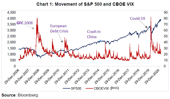 During the first week of February 2018, the global equity markets witnessed turbulence. With the release of high jobs figure in the US, portfolio rebalancing due to a rise in the bond yields brought about a fall in global stock markets. The market condition worsened with the failure of many complex volatility-linked funds. In India, the stock market was rising amidst high volatility towards the end of January 2018 but fell at the beginning of February 2018 alongside turbulence in global stock markets. This phenomenon was not unique to the Indian equity market; it resulted from a portfolio rebalancing away from emerging markets as an asset class. In consonance with it, the India VIX (IndVIX) increased sharply during this period and the IndVIX touched 20 on February 6, 2018. With a sharp correction in equity indices in February 2018, the inverse relationship got restored in the rest part of February 2018. The simultaneous rise in the Nifty and the IndVIX appeared again in April 2019. These two spells of a simultaneous rise in both stock index and volatility index cast some doubt on the generally perceived inverse relationship, and it has been a subject of research across countries. Some basic statistics are given in the table below on the stock markets in India and the US. The mean and standard deviation of both the volatility indices are nearly close to each other, indicating that both the markets have witnessed a mostly similar type of movement in the volatility indices (Table 1). | Table 1: Movement of Stock Index and Volatility Index | | INDIA | Nifty 50 Index | India VIX Index | | Period | Start | End | Start | End | Min | Max | Mean | Standard Deviation | | 2009-20 | 3033 | 13982 | 41 | 21 | 10 | 84 | 20 | 8.0 | | US | S&P 500 | CBOE VIX | | | Period | Start | End | Start | End | Min | Max | Mean | Standard Deviation | | 2009-20 | 932 | 3756 | 39 | 23 | 9 | 83 | 19 | 8.45 | | Source: Bloomberg; and Authors’ Estimates. | Furthermore, the scatter plots of the stock index and the implied volatility index are shown in Chart 3. The presence of a significant number of observations in the second and fourth quadrants highlights, prima facie, the negative relationship. But the presence of some observations in the first and third quadrants also marks time points in the market when the stock market and implied volatility index move in the same direction. On the whole, it suggests that while the general belief of the relationship being negative is persisting, there is an occasional unidirectional movement. The presence of these contrasting trends requires a more detailed analysis.  Over the period (2008-2020), the S&P 500 went up on 55 per cent of the number of trading days. The CBOE VIX and S&P 500 witnessed unidirectional movement in about 19 per cent of the days (Table 2). A look at the columns 5 and 6 in Table 2 suggests that over most part of this period, the co-movement in both has occurred on a limited number of days. In the case of the Indian stock market, during 2008-20, the Nifty 50 and IndVIX moved in the same direction only in 32 per cent of the number of days (Table 3). This strengthens the earlier impression that the inverse relationship between the volatility index and the stock market movement holds in the Indian context during the recent period. | Table 2: Days with SPX and CBOE VIX Movement in the Same Direction | | Period | Number of Trading Days | Average VIX Close | SPX Up / All Days# (%) | SPX Up and VIX Up / Days of SPX Up@ (%) | SPX Down and VIX Down / Days of SPX Down$ (%) | SPX and VIX in the Same Direction / All Days^^ (%) | | 1 | 2 | 3 | 4 | 5 | 6 | 7 | | 2008 | 253 | 32.7 | 50 | 8 | 13 | 11 | | 2009 | 252 | 31.5 | 56 | 15 | 26 | 20 | | 2010 | 252 | 22.5 | 57 | 18 | 19 | 19 | | 2011 | 252 | 24.2 | 55 | 15 | 20 | 18 | | 2012 | 250 | 17.8 | 53 | 24 | 20 | 22 | | 2013 | 252 | 14.2 | 59 | 21 | 17 | 20 | | 2014 | 252 | 14.2 | 57 | 18 | 19 | 18 | | 2015 | 252 | 16.7 | 47 | 9 | 17 | 14 | | 2016 | 252 | 15.8 | 52 | 22 | 23 | 23 | | 2017 | 251 | 11.1 | 58 | 26 | 24 | 25 | | 2018 | 251 | 16.6 | 53 | 17 | 24 | 20 | | 2019 | 252 | 13.8 | 60 | 20 | 18 | 19 | | 2020 | 253 | 22.8 | 57 | 17 | 19 | 18 | | 2008-20 | 2769 | 19.8 | 55 | 18 | 20 | 19 | Notes: # indicates the ratio of number of days when the market rose, to the total number of trading days. @ indicates a rise in the volatility index coinciding with the rise in the market. $ indicates a fall in the volatility index coinciding with a fall in the market. ^^ indicates ratio of number of days when both the market and volatility index go in the same direction to total number of trading days.
Sources: Bloomberg; and Authors’ Estimates. |
| Table 3: Days with Nifty and India VIX Movement in the Same Direction | | Period | Number of Trading Days | Average India VIX Close | Nifty Up/ All Days@@ (%) | Nifty Up and India VIX Up/ Days of Nifty Up! (%) | Nifty Down and India VIX Down/ Days of Nifty Down$$ (%) | Nifty and India VIX in the Same Direction / All Days** (%) | | 2008 | 244 | 39.4 | 48 | 32 | 39 | 36 | | 2009 | 243 | 37.3 | 55 | 26 | 35 | 30 | | 2010 | 252 | 21.8 | 55 | 26 | 27 | 27 | | 2011 | 247 | 23.8 | 43 | 21 | 24 | 23 | | 2012 | 250 | 19.7 | 56 | 31 | 35 | 33 | | 2013 | 250 | 18.9 | 50 | 34 | 33 | 34 | | 2014 | 244 | 17.1 | 58 | 39 | 41 | 40 | | 2015 | 248 | 17.6 | 49 | 33 | 35 | 34 | | 2016 | 247 | 16.6 | 53 | 25 | 37 | 31 | | 2017 | 248 | 12.6 | 56 | 34 | 32 | 33 | | 2018 | 246 | 15.1 | 54 | 35 | 33 | 34 | | 2019 | 245 | 12 | 53 | 30 | 37 | 33 | | 2020 | 252 | 21 | 59 | 26 | 33 | 29 | | 2008-20 | 3216 | 21.8 | 53 | 30 | 34 | 32 | Notes: Data for the year is based on the calendar year. @@ indicates number of days when market goes up to the total number of trading days. ! indicates when the volatility index rose along with the rise in the market. $$ indicates when the volatility index goes down in the days when the market goes down. **indicates when both market and volatility index go in the same direction to total number of trading days.
Sources: National Stock Exchange; Bloomberg; and Authors’ Estimates. | V. Empirical Findings on the Relationship between Stock Index and Volatility Index The present paper examines the relationship between Nifty 50 with IndVIX during 2011-2020; the descriptive statistics are given in Table 4. The Jarque-Bera test statistic indicates that the normality assumption is rejected for the data. The average returns on both the series (NIFTY 50 and IndVIX) are close to zero, indicating that the two series do not have any trend in their movements (for select abbreviations, see Appendix (A.3)). | Table 4: Descriptive Statistics | | | NIFTY 50 | NIFTY Return | IndVIX Return | IndVIX | | Mean | 8060 | 0.0004 | 0.00003 | 18.8 | | Median | 8035 | 0.0006 | -0.003 | 17.0 | | Maximum | 13982 | 0.084 | 0.50 | Rate 84.0 | | Minimum | 4544 | -0.139 | -0.41 | 10.0 | | Std. Dev. | 2365 | 0.011 | 0.05 | 6.56 | | Skewness | 0.28 | -1.01 | 0.52 | 3,2 | | Kurtosis | 1.8 | 17.87 | 10.6 | 22.6 | | Jarque-Bera | 199 | 25625 | 6707 | 45828 | | Probability | 0.0 | 0.0 | 0.0 | 0.0 | | Sum | 21995416 | 0.97 | -0.10 | 51342 | | Sum Sq. Dev. | 0.00 | 0.33 | 7.31 | 117272 | | Observations | 2729 | 2728 | 2730 | 2730 | | Source: Bloomberg; and Authors’ Estimates. | The relationship between Nifty 50 and IndVIX is examined in the framework of a two-stage ordinary least squares (OLS) regression analysis (as applied in Giot, 2003). This regression does not suffer from the endogeneity issue as VIX is derived from the out-of-the money options, whose prices are remotely connected with the share prices. Since an asymmetric relationship is observed in the data, i.e., the negative return in the stock index affects the change in the implied volatility index differently in comparison with the positive return in the stock index, dummy variables are used for the different returns for finding out their effects on change in IndVIX. The first-stage regression equation (1) is given below: In the second stage (equation 2), quadratic terms of Nifty returns are added in the above equation for looking into the influence of the return size on the change in the volatility index: The estimation is carried out with the application of the OLS Newey-West consistent standard errors, and the results show that the coefficients β1+ and β1- are different (Table 5). The Wald test result suggests that the coefficients are significantly different from each other. Since signs of both the coefficients are negative, the results confirm that a positive return decreases implied volatility while a negative return generates higher implied volatility. Further, β1- is larger in absolute value than β1+, highlighting that a falling stock market index generates a larger change in volatility as compared to a rising stock index. In the second stage of the regression, the size effect is clearly visible from the results of Equation 2. The coefficient of β2+ is positive, indicating that the size of positive returns can increase volatility. Since the absolute value of β2+ is bigger than β1+, it is inferred that once the size of the positive return reaches higher levels, the positive coefficient of β2+ can counter the negative coefficient of β1+ in equation 2, making the overall effect positive on the change in the volatility index, leading to a situation where a rise in the market gets associated with a rise in the volatility index. The coefficient β2- is significant in the case of NIFTY, indicating that the size of the negative return decreases the implied volatility index (IndVIX). While in general, a negative return increases implied volatility, once its size increases to a higher level, it decreases the implied volatility, creating a situation where a fall in the market gets associated with a fall in implied volatility. The US stock market also displayed similar behaviour, but the coefficients of the size of the return are larger than estimated in this paper for India. Results of Forward-Looking Regression Since volatility is an indicator of risk in the market, it generates a perception that its increase brings about market corrections. Hence, the focus here is to find out the connection of future stock index return with the present volatility level. The goal is to check whether a higher value of the volatility index signals an oversold market and whether any buy signals could be derived from the level of the volatility index. Table 6 suggests mixed signals in this regard. On the days when VIX reached the highest levels in the preceding two years, forward-looking returns remained positive in many of the subsequent days. The focus of the empirical exercise is to understand whether future stock market movements can be gauged from the present-day volatility index. The exercise is conducted to confirm the perception of the practitioners that a high level of implied volatility indicates an oversold condition in the market, and it could be a signalling tool for market purchases. Table 6: VIX Reached Higher Level than that of the Preceding Two Years
(Forward-Looking Returns in NIFTY 50) | | Dates | IndVIX | One-day | Five-day | Twenty -day | Sixty-day | | 23-Sep-2011 | 35.16 | -0.01 | 0.02 | 0.05 | -0.03 | | 26-Sep-2011 | 35.43 | 0.03 | 0.00 | 0.07 | -0.01 | | 4-Oct-2011 | 37.19 | 0.00 | 0.07 | 0.10 | 0.00 | | 21-Apr-2014 | 34.39 | 0.00 | -0.02 | 0.06 | 0.11 | | 8-Oct-2018 | 20.15 | 0.00 | 0.02 | 0.02 | 0.04 | | 11-Oct-2018 | 20.55 | 0.02 | 0.01 | 0.02 | 0.06 | | 22-Oct-2018 | 21.36 | -0.01 | 0.00 | 0.04 | 0.06 | | 15-Apr 2019 | 21.4 | 0.01 | 0.00 | -0.02 | -0.01 | | 16-Apr-2019 | 21.7 | 0.00 | -0.01 | 0.00 | -0.01 | | 18-Apr-2019 | 22.8 | -0.01 | 0.00 | 0.00 | -0.01 | | 22-Apr-2019 | 24.1 | 0.00 | 0.01 | 0.01 | 0.00 | | 23-Apr-1019 | 24.6 | 0.01 | 0.01 | 0.00 | -0.01 | | 6-May-2019 | 26.4 | -0.01 | -0.04 | 0.04 | -0.05 | | 7-May-2019 | 26.5 | -0.01 | -0.02 | 0.04 | -0.03 | | 13-May-2019 | 27.4 | 0.01 | 0.06 | 0.07 | -0.02 | | 15-May-2019 | 28.7 | 0.01 | 0.05 | 0.07 | -0.01 | | 9-Mar-2020 | 30.8 | 0.00 | -0.15 | -0.14 | -0.03 | | 11-Mar-2020 | 31.6 | -0.09 | -0.21 | -0.15 | -0.05 | | 12-Mar-2020 | 41.2 | 0.04 | -0.15 | -0.07 | 0.04 | | 13-Mar-2020 | 51.5 | -0.08 | -0.13 | -0.10 | -0.01 | | 16-Mar-2020 | 58.9 | -0.03 | -0.19 | 0.01 | 0.08 | | 17-Mar-2020 | 62.9 | -0.06 | -0.14 | 0.03 | 0.10 | | 18-Mar-2020 | 64 | -0.02 | -0.02 | 0.06 | 0.18 | | 19-Mar-2020 | 72.2 | 0.06 | 0.04 | 0.11 | 0.21 | | 24-Mar-2020 | 83.6 | 0.06 | 0.10 | 0.17 | 0.28 | | Source: Bloomberg; and Authors’ Estimates. | Giot (2003) made a forward-looking analysis of the implied volatility index and made a case that higher levels of the implied volatility index sent signals to traders about the buying points in the stock market. He studied whether the implied volatility index is a forward-looking indicator for undertaking investment in the stock market, by extending his own work of 2002 on the connection of the volatility index with the underlying stock index, taking data for Germany and the US. As noted earlier, we have applied his framework to the Indian stock market. The forward-looking returns are taken at the interval of one-day, five-day, 20-day, and 60-day, with the returns calculated in a forward-looking manner, i.e., n-day ahead return (Niftyt+1/Niftyt, Niftyt+5/Niftyt, Niftyt+20/Niftyt, and Niftyt+60/Niftyt). Then, these returns are calculated in a rolling way for every day till the end of the data points. For assessing the notion that very large volatility acts as buying points, the daily volatility index is demarcated by creating percentiles of the volatility levels. 20 percentiles are created by taking preceding data of the past two years up to t-1 data point. Daily IndVIXt is compared with these percentile figures, and suitably ranked. IndVIXt matching with the maximum percentile figure of the past two years is ranked as 20. When it is more than the maximum figure of the past two years, it is ranked at 21. This process helps in converting a qualitative measure to a quantitative measure (from IndVIXt at every level to the exact ranking of the IndVIXt). The ranks are calculated in a rolling way till the end of data points. 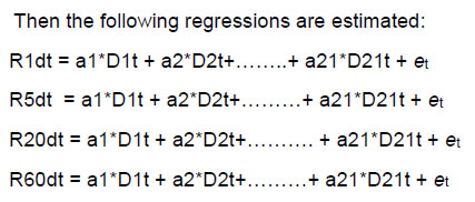 where, R1dt, R5dt, R20dt, R60dt are one-day, five-day, 20-day, and 60-day forward-looking returns, respectively. D1t is a dummy variable for IndVIXt ranked in the first percentile, and D1t takes the value of 1 if IndVIXt is in the first percentile, otherwise 0. All the IndVIXt are converted to one of the 21 dummy variables and are assigned figures (either 1 or 0) in this way. All the twenty-one dummy variables arrived on the basis of the IndVIXt level are used in the above regression equations. The coefficients of the dummy variables in the results are utilised to understand the effect of various ranks of the volatility index on the forward-looking returns. In this regard, Giot (2003) observes that high levels of the volatility index can be an indicator for taking long positions to derive positive future returns (the relevant table from the study is in Appendix (A.2)). On the opposite, long positions taken at a low level of implied volatility index are likely to generate negative future returns. | Table 7: Regression Results as per Trading Duration (INDIA-NIFTY) | | Dummy Variable | Forward-Looking Return | | One-day | Five-day | Twenty-day | Sixty-day | | D1t | 0.001(0.06) | 0.002(0.35) | 0.01(0.02) | 0.02(0.32) | | D2t | -0.0001(0.83) | 0.003(0.25) | 0.01(0.17) | 0.02(0.30) | | D3t | -0.001(0.21) | -0.006(0.04) | -0.01(0.41) | 0.001(0.97) | | D4t | -0.0001(0.93) | -0.001(0.84) | -0.01(0.25) | -0.002(0.93) | | D5t | -0.0003(0.67) | -0.001(0.62) | -0.01(0.31) | 0.007(0.67) | | D6t | 0.0001(0.87) | -0.001(0.65) | -0.01(0.55) | -0.007(0.72) | | D7t | -0.0(0.92) | -0.00(1.0) | -0.001(0.86) | -0.01(0.56) | | D8t | 0.0002(0.76) | -0.0002(0.93) | -0.01(0.12) | -0.01(0.48) | | D9t | -0.01(0.25) | 0.001(0.72) | 0.001(0.81) | 0.0002(0.99) | | D10t | 0.0005(0.52) | -0.001(0.75) | 0.003(0.68) | 0.02(0.19) | | D11t | -0.0(0.94) | 0.002(0.61) | 0.008(0.29) | 0.01(0.46) | | D12t | 0.002(0.06) | 0.005(0.07) | 0.009(0.24) | 0.02(0.17) | | D13t | 0.002(0.02) | 0.008(0.01) | 0.02(0.00) | 0.05(0.01) | | D14t | 0.0(0.92) | 0.002(0.50) | 0.01(0.07) | 0.05(0.06) | | D15t | -0.0001(0.87) | 0.001(0.73) | 0.01(0.25) | 0.05(0.06) | | D16t | -0.0004(0.03) | 0.002(0.57) | 0.009(0.38) | 0.03(0.14) | | D17t | 0.001(0.41) | 0.008(0.01) | 0.01(0.07) | 0.05(0.01) | | D18t | 0.0002(0.89) | 0.002(0.59) | 0.02(0.08) | 0.04(0.06) | | D19t | 0.002(0.13) | 0.006(0.34) | 0.03(0.02) | 0.08(0.01) | | D20t | 0.001(0.55) | 0.01(0.31) | 0.02(0.07) | 0.06(0.05) | | D21t | -0.002(0.74) | -0.02(0.42) | 0.02(0.06) | 0.04(0.07) | | Adjusted R2 | -0.002 | 0.02 | 0.04 | 0.08 | Note: The figures in different columns give the OLS coefficients for the dummy variables given in the first column. Figures in parentheses are p-values, and statistically significant ones are indicated in bold.
Sources: Bloomberg; and Author’s Estimates. | The regression results containing the effect of different levels of the volatility index on the forward-looking NIFTY 50 and S&P 500 returns are given in Tables 7 and 8, respectively. The explanatory variables do not have much explaining power as evident from low values of adjusted R2. However, there are some buying points that appear statistically significant, while there are virtually no selling points that are statistically significant. In the Indian case, the adjusted R2 of the regression is negative for forward-looking return at a 1-day interval which indicates that the explanatory variables do not have the power to explain the dependent variable, i.e., forward-looking return of 1-day duration. For the five-day return, the coefficients of the volatility index at 12, 13, and 17 levels are significant, with a rare selling point at level 3 which is also significant. When the volatility levels are ranked at 1, 13, 14, 17,18, 19, 20, and 21 these are buying points (having statistical significance) for return at 20-days forward-looking intervals. More buying points are also available for forward-looking investment at the duration of 60 days when the volatility indices are at 13, 14, 15, 17,18,19,20, and 21 levels. Overall, it says that when the volatility is at higher percentiles, it is a signal for buying at 20- and 60-day durations in the market. Many selling points appear at lower levels of volatility, but they are not statistically significant, except for one. In the case of the US stock market, the coefficient of the volatility index (at 10th level) is significant for the forward-looking return at a 1-day interval. The coefficients of volatility at 4, 11, and 13 levels are significant for the regression for forward-looking investment at 5-days duration. Further, the number of buying points increases with the increase in the investment horizon. When the volatility levels are at 1, 6, 12, 13, 14, 16, 17, 18, and 20, there are statistically significant buying points for investment at 20-days duration. More buying points are available for investment over the duration of 60-days, with most of them at higher percentiles. A comparison of Tables 7 and 8 indicates that when traders buy at a duration of 20-days and 60-days, high levels of volatility influence their decisions as many buying points appear at higher levels of volatility. The selling points (coefficients with negative signs) appear in the table at many levels of volatility, but the coefficients for those are not statistically significant. The latter is an unusual behaviour when compared with the result of Giot (2003), in which many statistically significant selling points appear at lower volatility levels. | Table 8: Regression Results as per Trading Duration (USA-S&P 500) | | Dummy Variable | Forward-Looking Return | | One-day | Five-day | Twenty-day | Sixty-day | | D1t | 0.00(0.80) | 0.001(0.41) | 0.01(0.08) | 0.02(0.06) | | D2t | 0.00(0.20) | 0.0002(0.91) | 0.003(0.45) | 0.02(0.03) | | D3t | -6.8e (0.86) | 0.001(0.52) | 0.004(0.31) | 0.004(0.76) | | D4t | 0.001(0.22) | 0.002(0.09) | 0.005(0.25) | -0.001(0.98) | | D5t | -0.0003(0.69) | 0.00(0.99) | 0.005(0.12) | 0.02(0.06) | | D6t | -0.0004(0.59) | -0.001(0.77) | 0.01(0.08) | 0.016(0.24) | | D7t | 0.0005(0.49) | 0.001(0.47) | 0.01(0.33) | 0.004(0.75) | | D8t | -0.0002(0.80) | 0.002(0.45) | -0.003(0.68) | 0.002(0.91) | | D9t | 0.001(0.40) | 0.002(0.34) | -0.003(0.77) | 0.02(0.21) | | D10t | 0.002(0.01) | 0.003(0.13) | -0.001(0.88) | 0.01(0.38) | | D11t | 0.001(0.35) | 0.004(0.06) | -0.002(0.79) | 0.008(0.59) | | D12t | 0.0015(0.03) | 0.001(0.50) | 0.009(0.07) | 0.01(0.38) | | D13t | 0.0004(0.57) | 0.004(0.06) | 0.015(0.00) | 0.03(0.08) | | D14t | 0.0001(0.91) | 0.004(0.21) | 0.014(0.01) | 0.02(0.09) | | D15t | -0.0005(0.70) | -0.001(0.88) | 0.005(0.44) | 0.02(0.10) | | D16t | 0.0007(0.39) | 0.002(0.52) | 0.02(0.00) | 0.04(0.00) | | D17t | 0.0011(0.36) | 0.001(0.73) | 0.014(0.08) | 0.05(0.00) | | D18t | -0.0002(0.90) | 0.004(0.30) | 0.016(0.06) | 0.05(0.00) | | D19t | 0.001(0.39) | 0.002(0.66) | 0.017(0.12) | 0.05(0.00) | | D20t | -0.00(0.97) | 0.01(0.16) | 0.023(0.02) | 0.06(0.00) | | D21t | 0.01(0.23) | -0.01(0.64) | 0.01(0.81) | 0.09(0.00) | | Adjusted R2 | 0.002 | 0.01 | 0.02 | 0.10 | Note: The figures in different columns give the OLS coefficients for the dummy variables given in the first column. Figures in parentheses are p-values, and statistically significant ones are indicated in bold.
Sources: Bloomberg; and Authors’ Estimates. | To sum up, both in India and the US, the volatility level influences the decision of traders to buy at a duration of 20-days and 60-days5. Since some high levels of volatility appear to give buying signals to investors, the findings can be viewed as empirical evidence against the concept of efficient markets. VI. Conclusion There is a conventional belief that the stock price index and the underlying implied volatility index move in opposite directions. However, on some occasions in the recent past, they displayed co-movements, casting doubts about the future course of action for investors. This paper explores various aspects of this relationship in the Indian context over a decade-long period and compares them with the available findings for the US. While the CBOE VIX and S&P 500 moved unidirectionally on only 19 per cent of the trading days during the period of the study, the India VIX and Nifty 50 moved in the same direction in only 32 per cent of the time, corroborating the presence of an inverse relationship between them. The findings of this paper indicate that a positive stock return is associated with a decrease in implied volatility, while a negative stock return is associated with a rise in the volatility index. Negative changes in the stock index generate much larger changes in implied volatility than positive changes. However, the size of return also plays a major role in influencing the relative change in stock market volatility. This size effect provides clues to the occasional rise of the stock market getting associated with a rise in the volatility index, as inferred from the statistically significant positive coefficients of the squared stock returns in the second stage equations of the regression analysis. The paper also examined in detail whether the implied volatility index can act as a forward-looking indicator for investment in the Indian stock market. The paper found that when traders go for buying at a duration of 20-days and 60-days, the volatility level influences their decision to an extent, as some of the buying points appear at higher levels of volatility. The selling points appear at many levels of volatility, but their coefficients are not statistically significant. This behaviour appears at variance with the results of Giot (2003), which had shown the presence of many buying points at higher volatility levels and many selling points at lower levels of volatility, that are statistically significant. However, Giot’s (2003) study was carried out by taking data for the pre-global financial crisis period. As part of the future research inquiry, the relationship studied in our paper can be tested using individual stocks. Furthermore, the study can be extended to see how the behaviour changes under different cyclical phases of the market.
References Bagchi, D. (2012). Cross-sectional Analysis of Emerging Market volatility Index (India VIX) with portfolio returns, Internal Journal of Emerging Markets, 7(4). Banerjee, P. S., Doran, J.S. & Peterson, D.R. (2007). Implied Volatility and Future Portfolio Returns, Journal of Banking and Finance, 31: 3183-3199. Black, F. (1976). Studies of Stock Market Volatility Changes. Proceedings of the American Statistical Association, Business and Economic Statistics Section, 177-181. Brandt, M. W., and Kavajech, K.A. (2004). Price Discovery in US Treasury Market, The impact of Oderflow and Liquidity on the Yield Curve, Journal of Finance, Vol 6. Chengli, Z. & Yinhong, Y. (2016). Relationship between Implied Volatility Index and its Underlying Market Index - Comparison between Chinese and American Market, International Conference on Applied Financial Economics, Shanghai. Chiang, S. M. (2012). The Relationships between Implied Volatility Indexes and Spot Indexes, Procedia - Social and Behavioral Sciences, 57: 231-235. Chicago Board Options Exchange. (2018). http://www.cboe.com/blogs/options-hub/2018/01/16/vol-411-follow-up-historical-look-at-spx-and-vix-moving-together. Dania, A. & Malhotra, D.K. (2014). Transmission of U.S. Stock Market Implied Volatility to Equity Markets of Emerging Countries, The Journal of Wealth Management Fall, 17 (2): 45-54. De Long, J.B., Shleifer, A., Summers, L.H., Waldmann, R.J. (1990), Noise trader risk in financial markets. Journal of Political Economy, 98(4):703–738. Ederington, L. H., & Guan, W. (2010). How asymmetric is U.S. stock market volatility? Journal of Financial Markets, 13, (2) 225–248. https://doi.org/10.1016/j.finmar.2009.10.001 Fama, E.F. (1965). The Behaviour of Stock Prices, The Journal of Business, 38(1): 34-105. Fleming, J., Ostdiek, B. & Whaley, R. E. (1995). Predicting stock market volatility: A new Measure. Journal of Futures Markets, 15 (3): 265-302. Florian A. (2015). The Causal Relationship between the S&P 500 and the VIX Index, Critical Analysis of Financial Market Volatility and Its Predictability, Spring Gabler. Galai, D. (1979). A proposal for indexes for traded call options. Journal of Finance, XXXIV (5): 1157-1172. Gammeltoft, N.& Vannucci, C. (2017). Is the VIX Being Gamed? A Sudden Swoon Has Traders Talking Again, from https://www.bloombergquint.com/markets/is-the-vix-being-gamed-a-sudden-swoon-has-traders-talking-again Gastineau, G. (1977). An index of listed option premiums. Financial Analysts Journal, 33 (3): 70-75. Giot, P. (2002). Implied Volatility Indices as Leading Indicator of Stock Index Return?, Discussion Core Paper No. 2002/50 Giot, P. (2003). On the relationship between implied volatility indices and stock index return, citeseerx.ist.psu.edu/viewdoc/download. Giot, P. (2005). Implied volatility Indexes and Daily value at Risk Models, The Journal of Derivatives, 12(4). Han, C.-H., H., Liu., W-H, & Chen T Y (2014). VaR/CVaR estimation under stochastic volatility model, International Journal of Theoretical and Applied Finance, 17(2). Hibbert, A. M., Daigler R. T.& Dupoyet B. (2008). A behavioral explanation for the negative asymmetric return–volatility relation, Journal of Banking & Finance, 32: 2254–2266. Kumar, S. S. S. (2010). The Behaviour of India's Volatility Index, Volume 2, Issue 2 from www.iimidr.ac.in/wp-content/uploads/The-Behaviour-of-Indias-Volatility-Index.pdf. Kumar, S.S.S. (2012). A first look at the properties of India’s volatility Index, The International Journal of Emerging Markets, 7(2):160-176. Mall, M., Mishra, S., Mishra, P.K. & Pradhan, B.B. (2014). A study on relationship between India VIX and Nifty returns, Intercontinental Journal of Banking, Insurance and Finance, 1(3). Monetary Policy Report, April 2018, Reserve Bank of India. Ominous sign! Nifty & VIX rising together; what is it saying really? (2019). The Economic Times, April 15, 2019. Padhi, P. & Shaikh, I. (2014). On the relationship of implied, realized and historical volatility: Evidence from NSE Equity Index Options, Journal of Business Economics and Management, 15(5): 915-934. Poterba,J. M. and Summers, L. H. (1987). Mean Reversion in Stock Prices: Evidence and Implications, NBER Working Paper, No. 2343. Ross, S. A. (1989). Information and Volatility, The no-arbitrage martingale approach to timing and resolution of insolvency, Journal of Finance, 44:1-17. Schwert, W. G. (1989). Why does stock market volatility change over time? Journal of Finance, Vol 44 (5): 1115-1153. Shaikh, I. & Padhi, P. (2016). On the relationship of implied volatility index and equity index returns, Journal of Economic Studies, 43(1): 27-47. Shaikh, I. (2018). Investors’ fear and Stock return: Evidence from National Stock Exchanges of India, Engineering Economics, 29(1): 4-12. Thenmozhi, M. & Chandra, A. (2013). Indian volatility index and Risk management in Indian stock market, NSE Working Paper, no.9. Thielen, B. (2016). Volatility and stock market returns: Can Volatility Predict Stock market returns?, Tilburg University. VIX and S&P500 in the Same Direction, http://www.macroption.com/vix-spx-same-direction/ Whaley, R.E. (2009). Understanding the VIX, The Journal of Portfolio Management, 35 (3): 98-105. What is India VIX really telling us? The Economic Times, April 15, 2019. White Paper on India VIX, National Stock Exchange. Yeh,J.H. & Tseng, J.C. (2007). Market Fear Gauge as the source of volatility Asymmetry - A New Perspective. Retrieved from https://citeseerx.ist.psu.edu/viewdoc/download?doi=10.1.1.297.5648&rep=rep1&type=pdf
Appendix A.1 The VIX Calculation The Indian VIX calculation is a replication of the CBOE VIX into the Indian market. The VIX calculation is done as described in the white paper released on it by the CBOE. The formula is described below. The stock index shows movements of the broader stock market and is calculated from the price of the selected scrips. However, the VIX is computed from the options’ order book. Therefore, Nifty is a number, whereas VIX is an annualised percentage. The formula used in the calculation6 is taken from NSE paper, and it is copied below from that white paper. T is Time to expiration F is the Forward Index taken as the latest available price of NIFTY future contract of corresponding expiry. Ki is the Strike price of ith out-of-the-money option; a call if Ki > F and a put if Ki < F;both put and call if Ki=Ko ΔKi is the Interval between strike prices- half the distance between the strike on either side of Ki: (Note: ΔK for the lowest strike is simply the difference between the lowest strike and the next higher strike. Likewise, ΔK for the highest strike is the difference between the highest strike and the next lower strike) R is a Risk-free interest rate to expiration Q (Ki) is Midpoint of the bid-ask quote for each option contract with strike Ki K0 First strike below the forward index level, F. More details on the symbols and calculation methodology are in the White Paper on India VIX, National Stock Exchange. | A.2 Regression Results as per Trading Duration (NASDAQ-100) | | Dummy Variable | Return
(One-day) | Return
(Five-day) | Return
(Twenty-day) | Return
(Sixty-day) | | D1t | -0.60 (0.20) | -1.84(0.96) | -6.14(1.38) | -21.81(2.39) | | D2t | -0.04 (0.37) | -0.61(1.03) | -4.46(2.03) | -14.73(2.80) | | D3t | 0.02 (0.40) | -0.48(0.69) | -4.90(1.93) | -15.01(3.03) | | D4t | -0.34 (0.39) | -2.06(1.07) | -8.00(2.78) | -6.11(3.03) | | D5t | -0.05(0.28) | -2.39(1.06) | -9.24(3.08) | -6.64(3.60) | | D6t | -0.22(0.52) | -0.55(1.01) | -3.34(2.89) | -6.60(4.46) | | D7t | -0.11(0.29) | 0.08(0.88) | -1.99(1.71) | -5.42(4.22) | | D8t | -0.12(0.30) | -0.70(1.27) | -0.39(2.73) | -4.97(4.27) | | D9t | -0.05(0.30) | 0(0.78) | -0.03(1.86) | -0.44(3.30) | | D10t | 0.13(0.29) | 0.44(0.84) | 2.50(1.80) | 4.67(3.55) | | D11t | -0.19(0.29) | -0.76(0.87) | 1.52(2.00) | 7.51(3.45) | | D12t | 0.05(0.38) | 1.17(0.70) | 1.69(1.54) | 6.98(3.20) | | D13t | 0.14(0.25) | 0.66(0.97) | 2.01(2.17) | 4.80(4.10) | | D14t | 0.07(0.33) | 1.01(0.75) | 2.02(1.82) | 1.92(4.22) | | D15t | 0.09(0.30) | 0.68(0.83) | 3.13(1.64) | 2.71(3.53) | | D16t | -0.16(0.31) | -0.54(0.93) | -0.28(1.55) | -1.24(3.67) | | D17t | 0.16(0.26) | -1.36(0.75) | 0.05(2.09) | 1.82(2.74) | | D18t | -0.14(0.23) | 0.63(0.72) | 3.27(1.73) | 7.45(2.55) | | D19t | 0(0.28) | 0.36(0.79) | 1.49(1.69) | 3.02(3.39) | | D20t | 0.35(0.23) | 1.15(0.89) | 1.20(1.89) | 1.57(3.84) | | D21t | 0.75(1.39) | 3.73(1.73) | 11.16(3.63) | 27.19(7.38) | | Note: The table has been taken from Giot (2003) paper just to illustrate how the trading strategy operated in case of NASDAQ100. Newey-West standard errors are given in parenthesis. The time period is June 2, 1997-January 31, 2003. | A.3 Select Abbreviations -
CBOE VIX = Chicago Board of Options Exchange’s Volatility Index -
DAX = Stock market index on the Frankfurt Stock Exchange -
IndVIX = India VIX -
RIndvixt = Relative Change in the India VIXt -
rniftyt = Return on NIFTY 50 -
S&P 500 = Standard and Poor's 500 -
SPX= S&P 500
|