Press Release
RBI Working Paper Series No. 02 Tail Risks of Inflation in India Silu Muduli and Himani Shekhar@ Abstract 1This paper estimates the tail risks of consumer price inflation in India using a quantile regression framework. It examines the impact of various domestic and global macroeconomic factors, along with the role of the flexible inflation targeting (FIT) in influencing the inflation tail risks as well as in explaining the shifts in its conditional distribution. A rise in domestic income and household inflation expectations, elevated global commodity prices - both fuel (i.e., crude oil) and non-fuel, and easy financial conditions pose upside risks to Consumer Price Index (CPI) headline inflation. The results also show that both lower and upper tail risks of inflation have stabilised in the FIT period and that the macroeconomic factors capture the tail risks to the inflation target band of 2 to 6 per cent in India reasonably well. JEL Classification: C21, C53, E31, P24, P44 Keywords: Inflation at risk, inflation uncertainty, monetary policy Introduction A precise estimate of the future inflation path and uncertainties around it is crucial for a proper assessment of inflationary conditions. During extreme events, such as the global financial crisis (GFC) and the COVID-19 pandemic, it becomes very difficult to predict the trajectory of inflation due to uncertainties surrounding it. In such circumstances, the distribution of future inflation, in addition to the inflation forecast, may be useful for future guidance, particularly under a flexible inflation targeting (FIT) framework. For India, food - a major component of the consumer price index (CPI) basket - typically has higher volatility owing to supply-side issues and the monsoon dependence of Indian agriculture. As a result, any disruption in weather patterns gets reflected in production, and in turn, prices. Extreme weather events namely, excess rains, deficient rains, floods, cyclones etc., bring additional uncertainty around the conditional mean trajectory of food inflation and makes it less reliable. Similarly, the high dependence of India on crude oil imports makes it susceptible to any global oil price shock. The uncertainty around food price inflation spills over to the uncertainty around CPI headline inflation as food occupies a significant proportion of the CPI basket and is also susceptible to many supply shocks. In such times of uncertainty, along with the mean path of future inflation, the distribution of inflation becomes crucial in the assessment of inflationary conditions. The inflation distribution may help in a proper assessment of the upside and downside risks to inflation. The upside and downside risks to inflation are known as Inflation at Risk (in notation, IaR) in the literature, a measure similar in notion and concept to Value at Risk (VaR) in financial risk-management theory to estimate the market and credit risk of a portfolio (Andrade, Ghysels, and Idier, 2012; Banerjee et al., 2020; López-Salido and Loria, 2020). The conventional approach assumes the symmetric distribution of errors around the mean path, which, however, may not always hold. Thus, the asymmetric nature of future inflation distribution may be useful in explaining the tail risks (i.e., the possibility of extreme values on either side) of inflation and in helping the monetary policy in communicating the balance of risks. Besides the asymmetry, understanding and accounting for the uncertainty around the central tendency are also crucial in stabilising inflation. Inflation uncertainty is one of the primary costs of inflation to the real economy as expected inflation is an important factor while making economic decisions. Uncertainty surrounding future inflation creates uncertainty regarding the future value of savings and investments, which in turn, may distort the efficient allocation of resources (Chowdhury, 2014). Consequently, inflation uncertainty can adversely affect consumption, investment, and growth. Since the monetary authority’s primary objective is to stabilise prices, it is also crucial to empirically examine whether it accounts for inflation uncertainty in monetary policy formulation. Given the importance of the distributional characteristics of inflation, the paper derives a conditional distribution of inflation which also indicates the balance of upside or downside risks. The paper has the following objectives: -
Estimate tail risks of inflation in India corresponding to various domestic and global drivers and test whether inflation risks have stabilised in the IT period; -
Examine shifting of the conditional distribution of inflation for different domestic and global shocks; -
Estimate expected tail values of inflation and examine the robustness of the models; -
Examine the causal relationship between inflation and inflation uncertainty and assess the reaction of the monetary policy to the asymmetric nature of conditional distribution and uncertainty around the central tendency. Estimations of conditional distribution and tail risks are based on a hybrid version of the standard New Keynesian Phillips Curve (NKPC) framework with financial conditions, crude oil price, and exchange rate of the Indian rupee (INR) vis-a-vis US dollar (USD) and global demand conditions- proxied by US real GDP growth as additional explanatory factors (Auer, Borio, and Filardo, 2017). The paper also examines the role of the IT framework in stabilising the tail risks. Therefore, the study includes both demand and supply-side factors in the estimation of the conditional distribution. In the Indian context, the existence of the Phillips curve has been established based on samples at national as well as sub-national levels in the post-GFC period (2007-09) (Behera, Wahi, and Kapur, 2018; Salunkhe and Patnaik, 2019). In this regard, a recent study by López-Salido and Loria (2020) concluded that tail risks are sensitive to domestic economic slack and have a significant role in influencing inflation distribution. Some recent studies have also considered the financial conditions index to examine the upside and downside risks to inflation during tight/easy financial conditions (Chevalier and Scharfstein, 1996; Gilchrist, Schoenle, Sim, and Zakrajšek, 2017). Chevalier and Scharfstein (1996) argue that during tight financial conditions, firms that face a higher constraint on accessing liquidity may set a higher price to increase their cash flow leading to higher inflation. India adopted the flexible IT framework in 2016, which was reviewed in March 2021, wherein the inflation target of 4 per cent with a ±2 per cent band around it was continued until the next review in 2026. During the period from 2011-12 to 2013-14, the average CPI-C inflation rate stood at 9.4 per cent, which moderated gradually towards the midpoint of the target band during the IT period. Notably, CPI-C inflation averaged 3.9 per cent during the IT phase of October 2016 – March 2020. RBI (2021) highlights the success of the framework in anchoring inflation expectations of both households and professional forecasters and lowering average inflation. Given the relevance of inflation projections in policy formulations, the RBI regularly publishes a fan chart of asymmetric inflation distribution based on a two-piece normal distribution which consists of two normal distributions below and above the mean (Banerjee and Das, 2011). Both the pieces have the same mean, but different standard deviations. This difference in standard deviations brings the asymmetry of a distribution around the mean. In the two-piece normal distribution, the values of standard deviations are derived from the past deviations from the forecast values, which incorporates asymmetry in the distribution. However, this paper derives the conditional distribution of inflation based on the estimated quantiles from quantile regression conditioned on the macroeconomic environment rather than depending on the past. Few recent studies in advanced economy central banks have highlighted the usefulness of conditional quantile regression in deriving the fan chart by incorporating expert judgements (for instance, see Sokol, 2021). Therefore, deriving the conditional distribution of inflation based on the current macroeconomic situation rather than depending on the past as in the case of a fan chart is the major contribution of this paper. The paper analyses the historical tail risks and shifts in the conditional distribution of inflation for various shocks. It concludes that a rise in domestic income and household inflation expectations increases the upside risks and lowers the downside risks to inflation. Elevated global commodity prices of both fuel (i.e., crude oil) and non-fuel, global economic growth and easy financial conditions raise the upside risks to inflation. Further, the results add to the success story of the adoption of the IT framework in India in stabilising CPI headline inflation as both lower and upper tail risks of inflation have stabilised in the IT period. Regarding the predictive efficiency of the models, the paper concludes that the models based on various macroeconomic factors capture the tail risks to the inflation target band of 2 to 6 per cent in India to a considerable extent. While examining the response of the monetary policy to asymmetry and uncertainty of inflation distribution, the paper finds evidence of tightening of the monetary policy during the periods of higher inflation uncertainty. The rest of the paper is organised as follows. Section II discusses the literature on the conditional distribution and tail risks associated with CPI-C inflation in India. Building on the literature and existing data sets, Section III presents a few stylised facts for inflation in India during the sample period and discusses the methodology used in the paper. Section IV presents the empirical results and also examines the asymmetry and uncertainty pertaining to inflation distribution and the response of the monetary policy to these. The last section concludes the paper with a few policy implications. II. Literature Review Studies that focus explicitly on the analysis of tail risks of inflation are relatively new in the literature (Banerjee, Contreras, et al., 2020; López-Salido and Loria, 2020). However, a few studies in the last decade analyse the quantiles of inflation and their dynamics; for instance, Wolters and Tillmann (2015) examine the persistence of different quantiles in the conditional distribution of inflation. Gupta, Jooste, and Ranjbar (2017) find higher persistence of inflation for higher quantiles in the case of South Africa. In related literature on convergence, Tsong and Lee (2011) in a study of 12 OECD countries find asymmetric convergence of inflation to long-run value post negative and positive shocks using the quantile regression approach. They find that positive shocks are more persistent than negative shocks and converge slowly to the long-run level. Similar empirical evidence is also seen in Uganda (Anguyo, Gupta, and Kotzé, 2020). Several studies have focussed on various determinants of inflation in a quantile regression framework; for instance, Iddrisu and Alagidede (2020) explain food inflation and its various determinants, such as economic growth, world food price inflation, monetary policy, etc., using quantile regression for South Africa. Lahiani (2019) explores the transmission of crude oil prices to different quantiles of overall prices for the US. Further, a plethora of studies have focused on the important determinants of conditional mean inflation using Phillips-curve specification and its different versions. Many of these studies find that the Phillips curve relationship estimated at the mean level weakened after the GFC (Blanchard et al., 2015). A few studies extend the NKPC estimation by incorporating global economic slack along with domestic economic slack to explain the domestic inflation dynamics (Auer, Borio, and Filardo, 2017). However, the evidence of global economic slack is mixed. For instance, Forbes (2019) finds significant evidence of the role of global economic slack on domestic inflation, while Mikolajun and Lodge (2016) find a limited impact of it on domestic inflation. Xu, Niu, Jiang, and Huang (2015) use non-linear quantile regression to estimate the Phillips curve for the US and conclude that the shape of the Phillips curve differs across quantiles. In the case of India, researchers find evidence for the existence of the Phillips curve based on samples from national and sub-national data in the post-GFC period (2007-09) (Behera, Wahi, and Kapur, 2018; Salunkhe and Patnaik, 2019). The above studies focus on exploring quantiles of inflation and do not explicitly mention the tail risks of inflation. Andrade et al. (2012) introduced an explicit analysis of tail risks of inflation i.e., “Inflation at Risk (IaR)” and used asymmetric property and distributional uncertainty to explain the monetary policy rule. The tail risks of inflation have been a major concern, particularly in advanced economies, in the post-GFC period (López-Salido and Loria, 2020). Some recent studies have also considered the financial conditions index to examine the upside and downside risks2 to inflation during tight/easy financial conditions (Chevalier and Scharfstein, 1996; Gilchrist, Schoenle, Sim, and Zakrajšek, 2017). Firms facing higher constraints on accessing liquidity during tight financial conditions and firms with weak balance sheets may set a higher price leading to higher inflation. In a recent study, Banerjee et al. (2020) use the volatility of asset prices as a proxy for tight financial conditions and find a significant impact of financial conditions on inflation. Some earlier studies based on quantile regression also find a positive association between stock market return and different quantiles of inflation in G7 countries (Alagidede and Panagiotidis, 2012). Inflation at Risk is similar to the concept of Value at Risk (VaR) in financial risk management, i.e., the extreme quantiles for a given level of probability. Among macroeconomic variables, a similar measure is also available for economic growth as Growth at Risk (Prasad et al., 2019). López-Salido and Loria (2020) in their study of advanced economies explicitly derived the conditional distribution based on quantiles. Banerjee et al. (2020) extended the analysis by including emerging economies and estimated the conditional density. Their study concludes that countries with IT show a relative moderation in inflation risks than non-IT countries. Banerjee, Mehrotra, and Zampolli (2020) model the impact of the COVID-19 pandemic and find higher upside and downside risks to inflation in emerging economies, and higher downside risks in the case of advanced economies. The advancement in deriving the conditional distribution based on quantile is a novel contribution in the above studies as compared to earlier studies that used quantile regression to study the quantiles of inflation and their dynamics. These studies highlight, in particular, the impact of different shocks on the tail risks of inflation. In our analysis, we augment the above-discussed analysis for India and examine certain country-specific features to explain the dynamics of tail risks of inflation. In related literature, Andrade et al. (2012) examine the response of the monetary policy to inflation asymmetry and uncertainty based on the professional forecasters’ survey data on inflation. A few studies explicitly analyse the relevance of inflation asymmetry on monetary policy formulation (Andrade et al., 2012; Evans, Fisher, Gourio, and Krane, 2016). Further, there exist several studies that discuss the causality and reverse causality between the level of inflation and inflation uncertainty (Cukierman and Meltzer, 1986; Sharaf, 2015; Su, Yu, Chang, and Li, 2017). According to Friedman (1977), higher average inflation causes uncertainty about future monetary policy responses, resulting in broad differences in actual and expected inflation, and therefore, leads to economic inefficiency making it detrimental to growth. This relationship was later formalised in a game-theoretic framework by Ball (1992) and the work is known as the Friedman-Ball hypothesis. On the contrary, Pourgerami and Maskus (1987) argue that inflation and inflation uncertainty have a negative relationship and reject the hypothesis of the deleterious effect of high inflation on price predictability as elevated inflation levels lead to the deployment of additional resources for lowering projection error resulting in better forecasts and hence reduction in inflation uncertainty. Coming to another dimension of a causal link from inflation uncertainty to inflation, Cukierman and Meltzer (1986) postulate that increased inflation uncertainty causes inflation to increase - the Cukierman-Meltzer hypothesis. When policymakers act with low credibility, the ambiguity of goals and poor quality of monetary control, then it may lead to an increase in the average inflation rate (Rojas, 2019). The flip side of this hypothesis is proposed by Holland (1995) who concludes that higher volatility of inflation reduces price levels reflecting policy makers’ motives for stabilisation. Further, sometimes the bidirectional relationship between inflation and inflation uncertainty is also observed under the Friedman-Ball hypothesis and the Cukierman-Meltzer hypothesis - higher inflation will increase the inflation uncertainty and vice-versa. In the case of India, Chowdhury (2014) finds evidence in support of this hypothesis using the generalised autoregressive conditional heteroscedasticity (GARCH) model. Kundu, Bhoi, and Kishore (2018) also present similar evidence between inflation and inflation volatility graphically at the sub-national level. Inflation uncertainty is a major concern for the monetary authority, as it assigns weights inter-temporarily to minimise its loss preference. Although not explicitly, a few studies have shown the detrimental effect of high inflation uncertainty on economic activity (Sauer and Bohara, 1995; Zhang, 2010). Hence, it becomes imperative for the monetary authority to reduce inflation uncertainty through appropriate policy instruments (Gan, Yee, Hadi, and Jalil, 2019; Zhang, 2010). In a standard monetary policy rule, besides output gap and inflation, studies have included exchange rate, global policy rate, and global economic growth to examine their impact on the monetary policy rate (Hutchison, Sengupta, and Singh, 2010; Reserve Bank of India, 2021). However, there are very few studies that explicitly model inflation uncertainty in the monetary policy rule to estimate its impact (Andrade et al., 2012). This paper adds to the limited literature in the Indian context on the importance of tail risks of inflation and their role in monetary policy. In this paper, we derive the conditional distribution of inflation based on the quantile regression in an NKPC framework that incorporates the macroeconomic environment. Further, we examine the role of distributional asymmetry and uncertainty in the monetary policy formulation. Our results support the causality between inflation and inflation uncertainty. III. Empirical Analysis III.1. Stylised Facts The uncertainty around food price inflation spills over to the uncertainty around headline inflation as food is a major contributor to CPI headline inflation variance (Chart 1)3. Within the FIT framework, price stability - avoiding high inflation rates or very low inflation rates over time - is the primary mandate for the RBI as volatile prices distort the economy’s price signals and may result in the misallocation of resources.  The CPI-C headline inflation has undergone significant changes in its distribution over the last decade in line with the evolving macroeconomic conditions (Chart 2a). Too high or too low inflation representing the upside and downside tail risks to inflation, respectively, is detrimental to RBI’s secondary objective of growth as well, and thus, requires a proper assessment of these risks. The FIT period coincided with a moderation in CPI inflation on the back of consecutive years of bumper food grains and horticulture production and relatively stable global commodity prices, particularly the crude oil. Irrespective of the broad easing of inflation, headline inflation deviated from the target, and went once below the lower bound of 2 per cent (in June 2017) and above the upper bound of 6 per cent consistently during December 2019-December 2020 mirroring the developments in food prices primarily owing to monsoon-related shocks and the COVID-19 pandemic-related supply disruptions (Chart 2b). 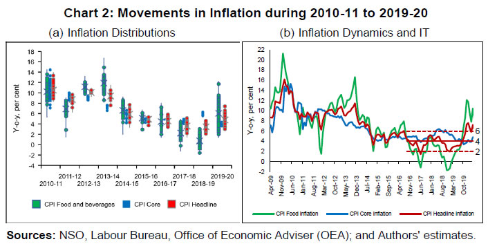 Given the high weight of food in the CPI basket, which is susceptible to adverse supply shocks, pressures in the food basket not only drives up the CPI headline inflation but also contributes substantially to its variance (Chart 3a and Chart 1). High levels of CPI inflation are often accompanied by higher volatility (Chart 3b). High inflation rates accentuate concerns about future inflation as they have the potential to influence long-term interest rates and generate uncertainty about the future value of the investment, savings, wages, tax rates, etc. In light of the fact that price stability is the primary objective of central banks, the volatility around the inflation path warrants the attention of the monetary authority. The asymmetry of distribution assumes greater importance given the fact that economic agents' expectations are influenced by the distribution of the realised inflation (RBI, 2021). III.2. Data and Summary Statistics This paper uses the monthly CPI-C inflation rate (y-o-y, per cent) from September 2009 to December 2019 (before 2011, CPI-IW (CPI Industrial Workers) is used). Table 1 presents the summary statistics of variables used in the paper. The CPI-C inflation averaged around 7 per cent during the sample. It remained above average during 2010-2012. It moderated subsequently to around 4 per cent with RBI’s formal adoption of the FIT framework in 2016, which was preceded by a transitional glide path from 2014-15. The one-year ahead median inflation expectations of households have been used as a proxy for a forward-looking measure of inflation expectations4 which averaged around 11.33 per cent during the sample. As households’ inflation expectations are observed quarterly, a cubic spline methodology has been employed to convert it into a monthly series (Stuart, 2018). Given the fact that the inflation expectations series is relatively persistent and stable, the above methodology might be a better approximation to obtain monthly frequency data. GDP growth at the constant market price has been used as a proxy for demand conditions in NKPC estimation (Banerjee et al., 2020). For real GDP growth, a similar methodology has been applied to adjust for the index of industrial production (IIP) and Purchasing Managers’ Index (PMI) composite indicator for India, which are observed every month and are coincident indicators of economic activities (see details of this interpolation in Appendix A2). In addition to these variables, NKPC estimation has been augmented with exchange rate, global commodity prices, financial conditions and global demand conditions to explain the inflation dynamics. On an average, the rupee has depreciated by 4 per cent vis-a-vis USD over the sample period with a very high degree of volatility. Commodity prices have been captured through Indian basket crude oil prices and global non-fuel commodity prices published by the IMF. To account for financial conditions, Citi financial conditions index (hereafter Citi FCI) for India has been used as a proxy for financial conditions, which has a relatively better forecasting power in predicting real economic activity (Hatzius et al., 2010). The Citi FCI consists of a weighted average of the following variables: corporate spreads, money supply, equity values, mortgage rates, the trade-weighted dollar, and energy prices. A higher value of Citi FCI indicates easy monetary conditions, and a lower value indicates a tight financial condition. To incorporate global demand, US real GDP growth has been considered. Moreover, we also analyse the importance given to inflation uncertainty and its distributional asymmetry in monetary policy formulation. For this purpose, the weighted average call rate (WACR) has been used as a proxy for the monetary policy rate. WACR is the operating target of the monetary policy, which is stable and symmetrically distributed at around 6.7 per cent. | Table 1: Summary Statistics | | Variables | N | Mean | Std. Dev. | Median | Kurtosis | Skewness | | CPI-C Headline Inflation | 124 | 6.99 | 3.36 | 5.92 | 2.51 | 0.52 | | 1-year Ahead Median Household Inflation Expectations | 124 | 11.33 | 2.47 | 11.18 | 1.8 | 0.25 | | Real GDP Growth Rate | 124 | 6.48 | 1.973 | 6.22 | 6.3 | 1.27 | | Exchange Rate Growth Rate | 124 | 3.99 | 7.47 | 3.36 | 2.87 | 0.52 | | Crude Oil Price Growth Rate | 124 | 5.81 | 32.45 | 3.2 | 2.82 | 0.3 | | Global non-fuel Price Index Growth Rate | 124 | 2.22 | 13.88 | -1.4 | 2.73 | 0.73 | | US Real GDP Growth Rate | 124 | 2.16 | 0.95 | 2.2 | 12.25 | -2.12 | | Citi FCI | 124 | -0.39 | 0.38 | -0.46 | 3.11 | 0.67 | | WACR | 124 | 6.76 | 1.43 | 6.72 | 3.34 | -0.51 | Notes: For definitions and sources, please see Appendix Table A1.
Source: Authors’ estimates. | III.3. Methodology The paper uses quantile regression to estimate the upper and lower tail risks. In a quantile regression, the quantiles of the dependent variable are explained by the set of explanatory variables. In an ordinary least square (OLS) regression, the estimated relationship is the average relationship between dependent and explanatory variables, whereas in the case of quantile regression the estimated relationship is for different specified quantiles. Thus, the benefit of using quantile regression is to estimate the role of explanatory variables in explaining extreme observations (or extreme quantiles) of the dependent variable. Since the study focuses on tail risks of inflation, quantile regression is an appropriate methodology to estimate the tail risks. Putting the quantile regression model more formally, for a dependent variable y explained by realised vector x, the quantile regression for pth quantile is given by,  In the later part of the paper, the conditional distribution has been estimated by minimising the sum of squares of the distance between the estimated quantiles from the quantile regression and quantiles derived from theoretical skewed distribution. The reason behind considering a skewed distribution is to provide space for the possible asymmetric feature of the conditional distribution. The paper considers a skewed normal distribution to estimate the smooth conditional distribution with asymmetric properties. The skewed normal distribution with parameters µ, δ, α, is given by IV. Results IV.1. Conditional Distribution and Tail Risks For analysing the tail risks, the paper considers four domestic factors: one-year ahead households’ inflation expectations based on the RBI survey; real GDP growth; exchange rate vis-à-vis US dollar; and crude oil prices. In addition to this, we have also examined the impact of financial conditions and the role of FIT on tail risks of inflation in the aftermath of its implementation. All the variables have been incorporated in the form of year-on-year percentage changes in the equations except inflation expectations (which already reflects y-o-y change) and Citi FCI. The FIT framework has been incorporated into the model through a dummy variable which takes the value of 1 after August 2016, and 0 otherwise5. The results of quantile regression are shown in Chart 4. The one-year ahead median household inflation expectations play a crucial role in CPI headline inflation dynamics. The impact of the inflation expectations is relatively less on lower tail risks and gradually increases for higher quantiles. The domestic real GDP growth has an impact on CPI headline inflation till the third quantile. The exchange rate has a positive effect on tail risks of inflation and a very limited effect at the median level though not significant. However, a time-varying plot of coefficients of exchange rate reveals that it broadly remained significant during 2015-2018 (Appendix Chart A4). The crude oil price has an impact on the median level and upper tail risks of inflation. Easy financial conditions have a positive influence on tail risks of inflation, and the sensitivity is relatively higher for upper tail risks. The introduction of the FIT dummy identifies the impact of FIT on CPI headline inflation tail risks. A negative coefficient of this dummy supports the success of the FIT framework. Since inflation was on a falling trend even before FIT adoption in India in 2016, the lower as well as the upper tail risks have come down by 3 percentage points. We estimate the tail risks of inflation based on the estimated parameters of domestic and global determinants of inflation. The tail risks are conditional on historical sample data with 5 per cent tails both in lower and upper tails. The lower tail risk (l(0.05)) is considered as a measure for downside risks to inflation, and the upper tail risk (u0.95) is considered to be upside inflation risks. The estimated tail risks are shown in Chart 5. The upper tail risks of CPI headline inflation fell to a level of around 7 per cent in 2019 from a level of 15 per cent in 2010. Similarly, the lower tail risks also went down to around 2 per cent in 2019 from 8 per cent in 2010. The downward shift in inflation tail risks could be partly attributed to the success of FIT and central bank credibility (Ayres et al., 2014). Importantly, the upper tail risks fell till 2016, and they remained around 7 per cent afterwards, whereas the lower tail risks continuously fell during the sample period. This means that during the FIT period, the downside risks were relatively higher compared to upside risks coming particularly from food reflecting successive years of bumper food grains and horticulture production. In the scenario analysis, we set preconditions on explanatory variables that influence the inflation dynamics. For simplicity, we assume data points of December 2019 as the preconditions. Next, we consider the standard deviation of the variables for one year before, i.e., January 2019 to December 2019. Then we provide one standard deviation shock to each explanatory variable and examine their impact on the conditional distribution of inflation one by one. 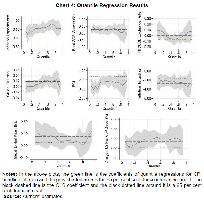 The reason for taking one standard deviation shock is to avoid extreme observation bias6. But in this case, we may consider extreme or rare events to study the impact on tail risks. So, we define the variables as of December 2019 as “before the shock”, and the variables that are considered for shock are added by a standard deviation to the values of December 2019 in the “after the shock” scenario. For instance, in the case of GDP growth shock, after the shock scenario will have all the variables the same as before the shock, and real GDP growth changes by one standard deviation of real GDP growth. In this way, we estimate the impact of different shocks on the conditional distribution of inflation. 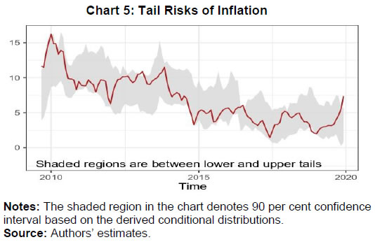 Domestic real GDP growth rate shock has a significant impact on the distribution and tails of CPI headline inflation as shown in Chart 6 and sign of their impact in Appendix Table A3. Median household inflation expectations have a uniform impact on the distribution of inflation as a rise in household inflation expectations lowers downside risks and increases upside risks. The exchange rate does not have any significant impact on the conditional distribution, but marginally reduces the lower tail risks. A one standard deviation shock in crude oil price increases risks on both sides and even the spread around mean inflation. Financial conditions shift the distribution of inflation asymmetrically with a relatively higher impact on upper tail risks. During loose financial conditions, the upside risks to inflation increase, while the downside risks to inflation decrease marginally. The previous section discussed shifts of conditional distribution for different shocks and their impact on the upside and downside risks of inflation. Besides this, it is also important to examine the expected value of inflation when it falls beyond the IaR. This is similar to the expected shortfall / conditional VaR in financial risk management. Here also, we define the similar notion, Here π0.05 and π0.95 are expected lower and upper tail inflation rates, respectively. These measures are coherent and spectral7. The IaR is a threshold value of tails for a given probability, while these measures are the average of inflation given that the inflation falls beyond the IaR threshold values. Therefore, this additional exercise provides estimates of the extent to which different shocks can impact the average tail values of inflation. The results of this estimation have been provided in Table 2. | Table 2: Expected Tail Inflation | | Shocks | π0.05 | π0.95 | | Baseline | 0.26 | 5.73 | | Real GDP growth | 0.54 | 5.91 | | Households’ inflation expectations (1-year ahead) | 0.48 | 5.85 | | Exchange rate | 0.11 | 5.51 | | Crude oil prices | 0.03 | 5.96 | | Citi FCI | 0.30 | 6.31 | | Global non-fuel inflation | 1.21 | 6.09 | | US real GDP growth | 0.73 | 6.69 | | Source: Authors’ estimates. | In the scenario analysis, before the shock refers to December 2019. At this point, the simulated results show that the lower expected value of CPI headline inflation is around 0.48 per cent, and the upper expected tail value is 6.04 per cent. In other words, given the domestic and global macroeconomic environment, if CPI headline inflation falls in the lower extreme regions, then it is expected to be around 0.48 per cent. Similarly, if the CPI headline inflation moves up unexpectedly due to some unforeseen events, then it is expected to be around 6.04 per cent. It is important to note that these values are based on a 90 per cent confidence interval and for a particular month. As mentioned in RBI (2021), the probability that inflation lies within the target is 80 per cent, which is also consistent with this analysis. IV.2. Inflation Target Range In the previous sub-sections, the paper estimated the tail risks of inflation for different kinds of macroeconomic shocks. In this sub-section, we discuss the ability of the above macroeconomic factors to predict breaching of the inflation target band, i.e., inflation above 6 per cent or below 2 per cent for the sample starting from January 2014, the starting phase of the glide path that proceeded the inflation targeting. To examine this, we estimate a simple probit model with dependent variables as a dichotomous variable which takes the value of 1 if inflation is above 6 per cent or below 2 per cent, otherwise takes the value of 0. For a more robust validation, we also consider the situation when the inflation does not fall in the 3 to 5 per cent category. The explanatory variables remain those considered in the quantile regression setup and based on the probit model, the breaching probability is estimated (shown in Charts 7a and 7b). To evaluate the efficacy of its prediction, the receiver operating characteristic (ROC) curve is utilised. The ROC curve plots the false positive rate (FPR or 1 − specificity) on the x-axis and the true positive rate (TPR or sensitivity) on the y-axis. The FPR represents the ratio of the total positive signal of breaching to total realised non-breaching cases. Similarly, TPR is the ratio of the total positive signal of breaching to the total realised cases of breaching. Hence, lower FPR and higher TPR imply better predictability of the model. In a graphical sense, the northwest direction is representing a better model. To quantify the above, area under the ROC curve (AUC) is used to identify a better model for classification. The AUC lies between 0 and 1. The AUC value of 0.5 indicates a random signal about the breaching, a value close to 0 indicates an inefficient model to correctly signal the breaching, and a value close to 1 indicates an efficient model that correctly predicts the breaching occurrence. The ROC curve is plotted in Chart 7c. Based on this Chart, when inflation breached the target range [2, 6], the model correctly predicts 94 per cent cases, while when it breached [3, 5] per cent, the model correctly predicts 74 per cent times. This directly measures the goodness of fit of the model and its predictability of tail risks about the inflation target range. Based on the evidence from the AUC value, this model can help in predicting the probability of inflation falling outside the comfort zone and thereby could be useful for inflation risk analysis. 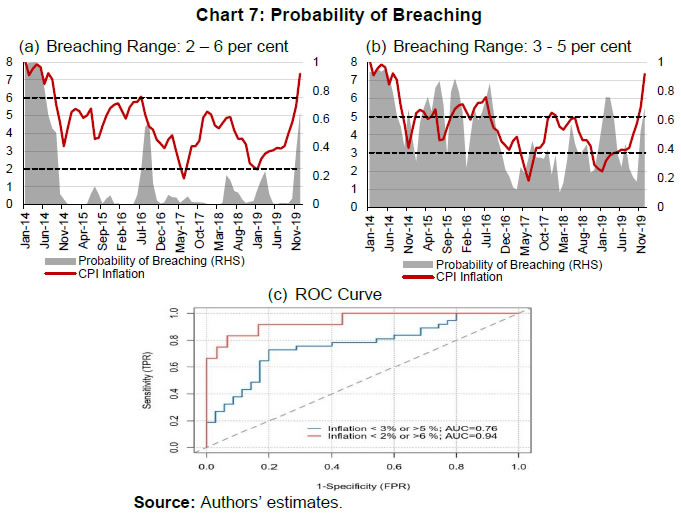 IV.3. Conditional Distribution of Inflation and the Monetary Policy After identifying and quantifying the tails risks emanating from key macroeconomic factors, it is pertinent to analyse their implications for monetary policy. In this regard, the literature has emphasised two aspects of inflation distribution - asymmetry and uncertainty – in the conduct of monetary policy (Andrade et al., 2012). Several studies assume a symmetric preference with a quadratic loss function with the dual objective of price stability and economic growth of the monetary authority. Therefore, the monetary authority reacts evenly to both positive and negative deviation of the inflation from the target. However, in contrast, few studies find an asymmetric reaction of monetary policy to the deviation of inflation from the target (Kilian & Manganelli, 2008; Ruge-Murcia, 2003). To examine the above asymmetric behaviour, this paper uses an asymmetry measure defined in the next section which indicates the skewness of the distribution. Similarly, the spread indicates the uncertainty of the random inflation values of the distribution and, therefore, the spread of inflation around its central tendency. In this analysis, first, we show the causal and instantaneous relationship between inflation and inflation uncertainty. Second, we investigate whether the monetary authority considers asymmetry and uncertainty surrounding inflation while framing the monetary policy. 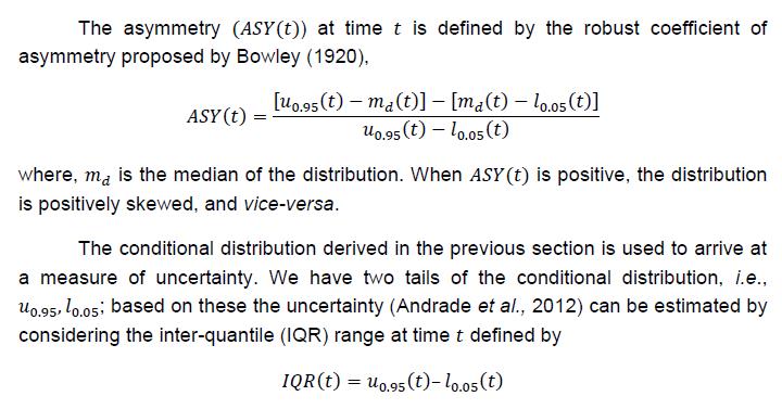
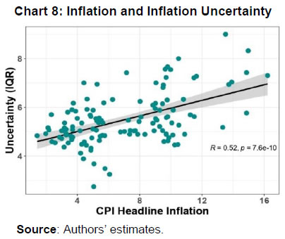 A scatter plot between inflation and inflation uncertainty shows a positive relationship between the two (Chart 8). This correlation, however, does not indicate causation. Therefore, we examine the relevance of two dominant hypotheses - Friedman-Ball hypothesis and Cukierman - Meltzer hypothesis - to identify the causal relationship between inflation and inflation uncertainty in India. Additionally, we also examine the instantaneous relationship as we consider the IQR of the conditional distribution as a measure of uncertainty instead of variance that depends on historical values. The above two hypotheses are generally based on the level and standard deviation of inflation. However, in this case, the uncertainty measure has been defined based on the prevailing macroeconomic conditions. For instance, there might be some kind of contemporary shock that may increase the spread and shift the distribution unevenly. Based on the Granger causality test, the CPI headline support only the Cukierman - Meltzer hypothesis, i.e., higher uncertainty is likely to result in higher inflation (Table 3). | Table 3: Results of Causal Relationships between Inflation and Inflation Uncertainty | | Null Hypothesis | Test | p-value | | Inflation does not cause uncertainty | Granger Causality | 0.19 | | Uncertainty does not cause inflation | Granger Causality | 0.03 | | No instantaneous relationship between inflation and uncertainty | Instantaneous | 0.07 | | Source: Authors’ estimates. | We now examine the role of distributional characteristics, i.e., asymmetry and uncertainty of inflation derived in the previous section in the monetary policy formulation. In a standard monetary policy rule, the policy rate is determined by the deviation of inflation from its target and output from its potential level. Since price stability is the primary objective of monetary policy, the measure of stability based on inflation uncertainty could also be a testable hypothesis in this context. Accordingly, two possible scenarios - low inflation with high volatility or high inflation with high volatility - can be introduced to the policy rule. As seen in the previous section, there is evidence of a positive instantaneous relationship between inflation and inflation uncertainty in India, and therefore, the first scenario is less likely to hold. Given the information content of uncertainty and asymmetry of inflation about realisations of future inflation, along with inflation, these two measures were augmented to estimate the monetary policy rule. We have considered the WACR, the operating target of the monetary policy as a proxy for the monetary policy rate, which is explained by CPI-C inflation, GDP growth, inflation uncertainty and asymmetry. Since there is an interdependence among policy rates, GDP growth, and inflation, the estimation using simple OLS may suffer from endogeneity issues leading to inconsistent estimates. Also, as there is evidence of a causal relationship between inflation and inflation uncertainty, this may lead to endogeneity for inflation uncertainty as well. To address the possible endogeneity problem, we have employed a generalised method of moments (GMM) instrumental variable regression with lags of explanatory variables as instruments. The results of the regression are shown in Table 4. The Hansen test based on J-statistics suggests the validity of the instruments used in the estimation, and robustness of estimation. | Table 4: Inflation Uncertainty, Asymmetry and the Monetary Policy | | | (1)
WACRt | (2)
WACRt | (3)
WACRt | | WACRt-1 | 0.953*** | 0.902*** | 0.889*** | | (0.0265) | (0.0277) | (0.0329) | | Real GDP Growtht-1 | 0.0248* | 0.0240* | 0.0188 | | (0.0138) | (0.0135) | (0.0148) | | Inflationt-1 | 0.0241*** | 0.0252*** | 0.0277*** | | (0.00814) | (0.00851) | (0.00918) | | Asymmetryt | 0.181 | - | -0.104 | | (0.180) | | (0.145) | | Uncertaintyt | - | 0.0860** | 0.0913** | | | (0.0369) | (0.0381) | | N | 117 | 117 | 117 | | R2 | 0.924 | 0.934 | 0.935 | | Hansen test p-value | 0.11 | 0.16 | 0.16 | Note: Standard errors in parentheses and * p < 0.1, ** p < 0.05, *** p < 0.01.
Source: Authors’ estimates. | The results show that WACR reacts positively to inflation uncertainty. A rise in uncertainty increases the policy rate by 9 basis points in the short run, and approximately by 90 basis points in the long run. On the other hand, results for asymmetry do not yield statistically significant results. V. Conclusions This paper investigates the tail risks of CPI-C inflation and their drivers. The paper derives the conditional distribution of inflation based on the current macroeconomic situation rather than depending on the past as in the case of a fan chart, which is the major contribution of this paper. The paper finds several insightful results that could be helpful in the proper assessment of inflationary conditions, particularly during uncertain times. The estimates suggest that tail risks of inflation have come down during the FIT framework. Further, the upside risks to CPI inflation have been relatively more volatile than the downside risks to inflation. In the FIT period, upside risks to CPI headline inflation have declined to a level of 6.5 per cent from a double-digit level preceding it and have remained stable. Since there is a downward shift in the conditional distribution, the downside risks to inflation have increased and have remained around 1.5 per cent. While examining the shift of the conditional distributions of inflation in response to various domestic and global shocks so as to analyse tail risks of CPI-C inflation, this study reveals that an increase in household inflation expectations, domestic real GDP growth, and global non-fuel price inflation uniformly shifts the distribution to right, leading to the higher upside and lower downside risks to inflation. Easy financial conditions have an asymmetric impact on the conditional distribution, particularly raising the upside risks to inflation. The exchange rate does not shift the conditional distribution significantly. Given the macroeconomic environment as of December 2019, the average lower and upper tail values of CPI headline inflation are 0.48 per cent and 6.04 per cent, respectively. Based on inflation and inflation uncertainty, proxied by the interquartile range of 95th and 5th quantile, the paper finds that inflation uncertainty causes higher CPI-C inflation, but not vice-versa, supporting the Cukierman - Meltzer hypothesis. The paper also finds a positive instantaneous relationship between inflation and inflation uncertainty. Furthermore, the paper concludes that the models based on the underlying macroeconomic factors fairly capture the tail risks to the inflation target band of 2 to 6 per cent in India.
References Alagidede, P., & Panagiotidis, T. (2012). Stock returns and inflation: Evidence from quantile regressions. Economics Letters, 117(1), 283–286. Andrade, P., Ghysels, E., & Idier, J. (2012). Tails of Inflation Forecasts and Tales of Monetary Policy. UNC Kenan-Flagler Research Paper No. 2013-17. Anguyo, F. L., Gupta, R., & Kotzé, K. (2020). Inflation dynamics in Uganda: a quantile regression approach. Macroeconomics and Finance in Emerging Market Economies, 13(2), 161–187. Auer, R., Borio, C. E. V, & Filardo, A. J. (2017). The globalisation of inflation: the growing importance of global value chains. BIS Working Papers No 602. Ayres, K., Belasen, A. R., & Kutan, A. M. (2014). Does inflation targeting lower inflation and spur growth? Journal of Policy Modeling, 36(2), 373–388. Ball, L. (1992). Why does high inflation raise inflation uncertainty? Journal of Monetary Economics, 29(3), 371–388. Banerjee, N., & Das, A. (2011). Fan chart: Methodology and its application to inflation forecasting in India. RBI Working Paper Series No. 05. Banerjee, R. N., Contreras, J., Mehrotra, A., & Zampolli, F. (2020). Inflation at risk in advanced and emerging economies. BIS Working Papers No 883. Banerjee, R. N., Mehrotra, A., & Zampolli, F. (2020). Inflation at risk from Covid-19. BIS Bulletin No 28. Barth III, M. J., & Ramey, V. A. (2001). The cost channel of monetary transmission. NBER Macroeconomics Annual, 16, 199–240. Behera, H., Wahi, G., & Kapur, M. (2018). Phillips curve relationship in an emerging economy: Evidence from India. Economic Analysis and Policy, 59, 116–126. Blanchard, O., Cerutti, E., & Summers, L. (2015). Inflation and activity--two explorations and their monetary policy implications. IMF Working Paper WP/15/230. Bowley, A. L. (1920). Elements of statistics (Issue 8). PS King. Chevalier, J., & Scharfstein, D. (1996). Capital-Market Imperfections and Countercyclical Markups: Theory and Evidence. American Economic Review, 86(4), 703–725. Chowdhury, A. (2014). Inflation and inflation-uncertainty in India: the policy implications of the relationship. Journal of Economic Studies. Christiano, L. J., Eichenbaum, M. S., & Trabandt, M. (2015). Understanding the great recession. American Economic Journal: Macroeconomics, 7(1), 110–167. Cukierman, A., & Meltzer, A. H. (1986). A theory of ambiguity, credibility, and inflation under discretion and asymmetric information. Econometrica: Journal of the Econometric Society, 1099–1128. Evans, C., Fisher, J., Gourio, F., & Krane, S. (2016). Risk management for monetary policy near the zero lower bound. Brookings Papers on Economic Activity, 2015(1), 141–219. Forbes, K. J. (2019). Has globalization changed the inflation process? BIS Working Papers No 791. Friedman, M. (1977). Nobel lecture: inflation and unemployment. Journal of Political Economy, 85(3), 451–472. Gan, P., Yee, K., Hadi, F., & Jalil, N. (2019). Monetary policy reaction function and external economic uncertainty: evidence from 30 selected countries. Management Science Letters, 9(8), 1207–1220. Gilchrist, S., Schoenle, R., Sim, J., & Zakrajšek, E. (2017). Inflation dynamics during the financial crisis. American Economic Review, 107(3), 785–823. Gupta, R., Jooste, C., & Ranjbar, O. (2017). South Africa’s inflation persistence: A quantile regression framework. Economic Change and Restructuring, 50(4), 367–386. Hatzius, J., Hooper, P., Mishkin, F. S., Schoenholtz, K. L., & Watson, M. W. (2010). Financial conditions indexes: A fresh look after the financial crisis. NBER Working Paper 16150. Holland, A. S. (1995). Inflation and uncertainty: tests for temporal ordering. Journal of Money, Credit and Banking, 27(3), 827–837. Hutchison, M. M., Sengupta, R., & Singh, N. (2010). Estimating a monetary policy rule for India. Economic and Political Weekly, 45(38), 67–69. Iddrisu, A.-A., & Alagidede, I. P. (2020). Monetary policy and food inflation in South Africa: A quantile regression analysis. Food Policy, 91, 101816. Kilian, L., & Manganelli, S. (2008). The central banker as a risk manager: Estimating the Federal Reserve’s preferences under Greenspan. Journal of Money, Credit and Banking, 40(6), 1103–1129. Kundu, S., Bhoi, B. B., & Kishore, V. (2018). Regional Inflation Dynamics in India. RBI Bulletin, 72(11), 57–66. Lahiani, A. (2019). Exploring the inflationary effect of oil price in the US: A quantile regression approach over 1876-2014. International Journal of Energy Sector Management. López-Salido, D., & Loria, F. (2020). Inflation at Risk. Finance and Economics Discussion Series 2020-013. Washington: Board of Governors of the Federal Reserve System, https://doi.org/10.17016/FEDS.2020.013. Mikolajun, I., & Lodge, D. (2016). Advanced economy inflation: the role of global factors. ECB Working Paper Series No 1948. Milgrom, P., & Roberts, J. (1982). Limit pricing and entry under incomplete information: An equilibrium analysis. Econometrica, 50(2), 443–459. Pourgerami, A., & Maskus, K. E. (1987). The effects of inflation on the predictability of price changes in Latin America: some estimates and policy implications. World Development, 15(2), 287–290. Prasad, A., Elekdag, S., Jeasakul, P., Lafarguette, R., Alter, A., Feng, A. X., & Wang, C. (2019). Growth at risk: Concept and application in IMF country surveillance. International Monetary Fund. Reserve Bank of India. (2021). Report on Currency and Finance. Rojas, E. R. (2019). Inflation and inflation uncertainty in selected Latin American countries. Problemas Del Desarrollo, 50(198), 113–144. Ruge-Murcia, F. J. (2003). Inflation targeting under asymmetric preferences. Journal of Money, Credit and Banking, 763–785. Salunkhe, B., & Patnaik, A. (2019). Inflation dynamics and monetary policy in India: A new Keynesian Phillips curve perspective. South Asian Journal of Macroeconomics and Public Finance, 8(2), 144–179. Sauer, C., & Bohara, A. K. (1995). Monetary policy and inflation uncertainty in the United States and Germany. Southern Economic Journal, 62(1), 139–163. Sharaf, M. F. (2015). Inflation and inflation uncertainty revisited: Evidence from Egypt. Economies, 3(3), 128–146. Sokol, A. (2021). Fan charts 2.0: flexible forecast distributions with expert judgement. ECB Working Paper No. 2624. Stuart, R. (2018). A quarterly Phillips curve for Switzerland using interpolated data, 1963--2016. Economic Modelling, 70, 78–86. Su, C.-W., Yu, H., Chang, H.-L., & Li, X.-L. (2017). How does inflation determine inflation uncertainty? A Chinese perspective. Quality \& Quantity, 51(3), 1417–1434. Tsong, C.-C., & Lee, C.-F. (2011). Asymmetric inflation dynamics: evidence from quantile regression analysis. Journal of Macroeconomics, 33(4), 668–680. Wolters, M. H., & Tillmann, P. (2015). The changing dynamics of US inflation persistence: A quantile regression approach. Studies in Nonlinear Dynamics \& Econometrics, 19(2), 161–182. Xu, Q., Niu, X., Jiang, C., & Huang, X. (2015). The Phillips curve in the US: A nonlinear quantile regression approach. Economic Modelling, 49, 186–197. Zhang, C. (2010). Inflation uncertainty and monetary policy in China. China & World Economy, 18(3), 40–55.
Appendix | Table A1. Variable Definition | Variables | Definitions | Data Source | | CPI Headline inflation | Year on year change in the consumer price index (CPI) | Ministry of Statistics and Programme Implementation and Labour Bureau, Ministry of Labour and Employment for data before 2011 | | 1-year ahead median household inflation expectations | A survey-based households’ inflation expectations measure based on different cities of India | Reserve Bank of India | | Global non-fuel commodities inflation | Year-on-year change in global non-fuel price index, which includes precious metal, food and beverages and industrial inputs price indices. | International Monetary Fund | | Real GDP growth rate | Year-on-year change in Gross Domestic Product (GDP) at constant market prices | Ministry of Statistics and Programme Implementation | | Exchange rate | The forex market exchange rate of rupee for one US dollar | Reserve Bank of India | | Crude oil price growth rate | The growth rate of crude oil (Indian Basket) prices | Petroleum Planning and Analysis Cell (PPAC), Government of India | | US real GDP growth rate | Year-on-year change in US real GDP at constant prices | U.S. Bureau of Economic Analysis | | Citi Financial Conditions Index | The weighted average of corporate spreads, money supply, equity values, mortgage rates, the trade-weighted dollar, and energy prices | Bloomberg | | Weighted Average Call Rate (WACR) | Short-term interbank market rate | Reserve Bank of India | A2. Interpolation of GDP Growth In India, the real GDP growth rates are observed quarterly. In the study, we need monthly series of real GDP growth. Note that quarterly GDP growth reflects the rise or fall of economic activity in the corresponding three months compared to the same three months in the previous year. A simple cubic spline interpolation of the quarterly GDP growth rate at time t, say gt (monthly) will reflect the change in economic activity in the time interval [t – 2, t] with respect to [t – 14, t – 12] in the previous year. The trend of this polynomial interpolated monthly GDP growth rate may deviate from the actual trend of economic activity that happened during the three months. To adjust for this trend, actual monthly proxies of economic activities during the month may be useful. The growth rate in the Index of Industrial Production (IIP) and Purchasing Managers’ Index (PMI) composite indicator has been considered to adjust the trend. The growth of IIPt and PMIt at the time reflects the increase in economic activity at time periods t and t – 12. The following steps are followed to obtain the monthly real GDP growth rate. 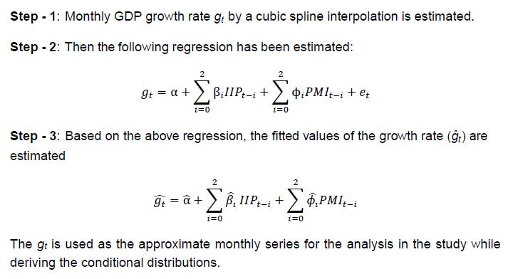
| Table A3. Impact of Different Explanatory Variables on Select Quantiles of Inflations | | Impact on CPI C Inflation | Lower Tail (0.05) | Median Quantile (0.5) | Upper Tail (0.95) | | 1 year ahead inflation expectations | + | + | + | | Domestic GDP | + | + | + | | Exchange rate (INR/USD) | + | - | + | | Crude oil | - | + | - | | FCI | + | + | + | | FIT | - | - | - | | Global non-fuel | + | + | + | | US GDP | + | + | + | | Source: Authors’ estimates. |
|