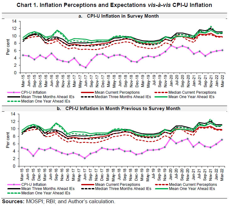
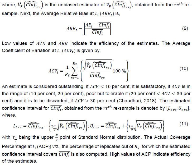
Press Release

RBI Working Paper Series No. 05

Reading Consumers’ Minds: An Analysis of Inflation Expectations

Purnima Shaw^@

Abstract

¹ The heterogeneity in the consumption baskets of households is often deemed responsible for the deviation of households’ inflation expectations from the headline inflation number. A novel approach is proposed in this paper to verify this by simulating heterogeneous population consumption baskets and estimating the mean inflation by sampling the baskets. The estimated mean inflation, treated as inflation sentiment, fails to display closeness with the survey numbers. Therefore, the paper proposes alternative logical methods for designing basket compositions and identifies the most suited method using which the estimated expectations are found to be close to and well-correlated with survey numbers. Such an attempt to find out the source(s) of disagreement in inflation expectations with respect to official inflation can be useful in understanding consumers’ inflationary expectations better for inflation analysis. The findings suggest that a sudden rise in inflation in items of regular use can explain the deviation in households’ inflation expectations from the official inflation. The deviation of survey expectations from the headline inflation can, thus, be explained effectively, over and above the other factors viz., demographic characteristics and exposure to media reports, which influence the formation of inflation expectations.

JEL Classification: D84, E20, E21, E30, E31

Keywords: Consumer price index, consumption basket, inflation, inflation expectations, sampling

Introduction

Inflation expectations are vital for monetary policy communication, as they affect the wage-setting behaviour, consumption, expenditure, investment, financial savings, etc. Hence, inflation targeting can be regarded as successful if the expectations of the economic agents are anchored effectively. Anchored inflation expectations reflect the trust of economic agents in central banks. The empirical measures of inflation expectations, therefore, form an important parameter in gauging the credibility of central banks. For this, the data on consumers sentiments need to be analysed carefully, including the shocks impacting households’ inflation expectations.

Variations in households’ consumption baskets are often deemed responsible for the deviation of their inflationary expectations from the official inflation numbers. However, this has not been verified empirically in the literature. It is anticipated that mean inflation in simulated heterogeneous consumer baskets should be well-correlated and close to the survey-based expectations. We design a novel approach to verify this empirically. A large number of heterogeneous consumption baskets are simulated. Treating this as the population, the mean inflation in the population baskets is estimated. The estimated mean inflation in the population baskets assumed as the simulated inflation sentiment fails to display a closeness with the survey numbers. Therefore, this paper explores alternative ways for simulating consumption baskets to find a logical method by which the simulated sentiments are closely related to the survey-based sentiments. The analysis helps to provide insights into the minds of consumers/ households as they form their expectations. This attempt to identify the source(s) of disagreement in inflation expectations with respect to the official inflation can help in better understanding and using the consumers’ inflationary expectations.

Section II of this paper provides a study of the existing literature on the disagreement in survey-based expectations with respect to the official inflation. Section III starts with the presumption that heterogeneous consumption baskets is the main reason for such a deviation. It develops a logical method to simulate heterogeneous consumption baskets to form a population of baskets, and then, sample the baskets from this simulated population. We then proceed to test the initial presumption empirically. On finding limited empirical evidence to support this presumption, we develop other logical methods of simulating the consumption baskets. The motive is to find the best logical method for simulating the consumption baskets such that the estimated inflation would be close in number bearing a high correlation with the survey-based sentiments. Section IV examines the proposed logics numerically using the Consumer Price Index (CPI) basket. Section V concludes.

II. Literature Review

Flexible inflation targeting critically hinges on measures to enhance agents’ confidence in central banks. Forward-looking monetary policies aim to study the future inflation dynamics by feeding forward-looking inflation expectations into the New Keynesian Phillips Curve (NKPC). However, expectations may not be perfectly rational, and hence, may not fit the NKPC. Hence, the empirical studies for most inflation targeting countries use a hybrid version of NKPC taking both forward and backward-looking components (Taylor, 1982; Gali and Gertlar, 1999 and Pattanaik et al., 2020). Another way of visualising the future price levels is using the well-known Dynamic Aggregate Demand – Surprise Aggregate Supply (DAD-SAS) model by which forward-looking (rational) inflation expectations assure an economy to reach the potential output level relatively faster than that of the backward-looking expectations through the wage channel (Alpanda et al., 2013 and Man and Peterson, 2019).

Inflation expectations of agents can be influenced by various factors. For instance, Murphy and Rohde (2018) opine that food prices are weighted more heavily by consumers than other consumer goods in the US. Zhao’s (2021) analysis brings out how inflation expectations of the US consumers is impacted by their sentiments on the prevailing economic conditions, their memory about news reports, and their social and demographic characteristics. Ciro and Zapata (2019) state that the disagreements in inflation expectations increase due to inflation volatility.

The Reserve Bank of India (RBI) has been tracking inflationary sentiments of households by conducting the Inflation Expectations Survey of Households (IESH) on a bimonthly basis in 19 cities in India. Generally, these expectations are in disagreement with the official CPI inflation. The correlations of households’ expectations for different lags (0, 1 and 2) and leads (0 and 1) of the CPI-Urban (CPI-U) inflation are shown in Table 1. The gap between households’ inflation expectations and the CPI-U inflation is also tabulated. A high and significant correlation is preferred. A significant gap between the CPI-U inflation and the expectations is not desirable. It is observed that although the correlations are significant, the gaps between actual and estimated sentiments are in the range of 3.5 to 5.1 percentage points (Table 1 and Chart 1).

India is not the only country showing a disagreement in survey-based inflation expectations with respect to the official inflation. It has been proven recently that such a disagreement exists in several other economies; India, in fact, is similar to Russia in this regard (Singh et al., 2022). Shaw (2019) took an empirical Bayesian approach to handle this disagreement for predicting the future inflation trajectory in the Indian case.

Considering the pattern of private final consumption expenditure (2011-12), it is observed that per capita consumption on health, transport services and education increased (Chart 2). However, these changes are not reflected in the consumption weights in official inflation. Changes in consumption pattern may also be one of the factors responsible for disagreement in households’ inflation expectations with respect to the official inflation.

Other factors, such as differences in consumption baskets, demography of consumers and exposure to media can also induce heterogeneity in households’ inflationary sentiments. Some of these factors are documented in the literature from other economies. For example, Souleles (2004) shows the systemic correlation between consumers’ inflation forecast errors and their demographic characteristics. About media exposure, Carroll (2003) is of the view that the stickiness in consumers’ inflation expectations is due to their infrequent attention to media reports. Ehrmann et al. (2015) identified socio-economic factors viz., income, age, gender and buying attitudes of consumers as crucial determinants of inflation expectations. This paper focuses on an important factor, as identified in the literature, namely, the differences in households’ consumption baskets in explaining the disagreement in inflation expectations with respect to the official inflation.

III. Methodology

In the following paragraphs, we propose different methods for simulating a population of consumption baskets; each one of these methods is based on different logic and set of assumptions.

III.1 Method 1

III.1.i Sampling and Estimation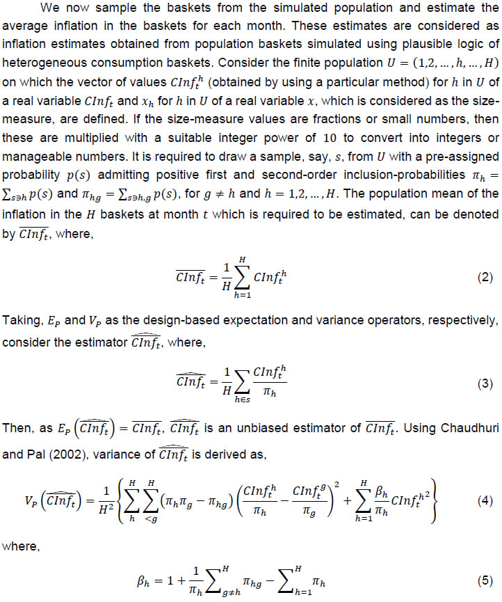

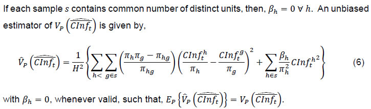In reality, while conducting the survey for estimating inflation perceptions and expectations of the households, it may be useful to sample the households using varying probability sampling schemes so as to make the sample more representative. However, the motive here is not to estimate representative inflation expectations, but to prove that the estimated inflation figures using simulated population baskets (following the logic of heterogeneity in the consumption baskets), deviate from the official inflation figures, i.e., they are close and well-correlated to the currently published households’ inflation expectations. Hence, the estimates that would be derived using the sample of consumption baskets drawn from the simulated population baskets would not be sampling-scheme specific. In fact, the motive here is to show that the disagreement in households’ inflation expectations with respect to the official inflation can be explained by estimating inflation from consumption baskets sampled by employing a general sampling scheme from a heterogenous population of consumption baskets simulated using a particular logic of select items.

III.1.ii Testing the Performance of Method 1

In order to demonstrate that huge variation in households’ consumption baskets is one of the crucial factors responsible for the deviation of their inflationary expectations from the official inflation numbers, the above simulation method is followed for 299 consumer items in the CPI basket.² However, due to the lack of continuous time series inflation data of 13 consumer items viz., “jackfruit”, “singara”, “mango”, “kharbooza”, “pears/ nashpati”, “berries”, “leechi”, “chips (gm)”, “sewing machine”, “electric iron, heater, toaster, oven and other electric heating appliances”, “VCD/ DVD hire (incl. instrument)”, “cinema: new release (normal day)” and “library charges”, 286 items are considered. The following steps³ are followed: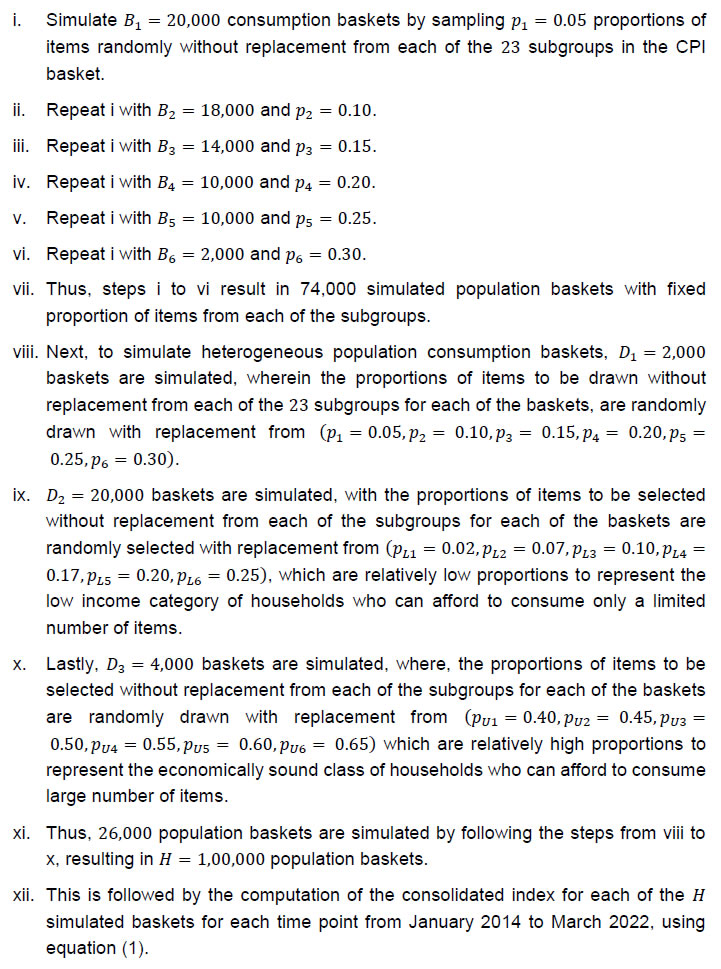

Next, a sample, say, s of baskets, of size n(≥2)=100⁵ is drawn from the population baskets using random sampling schemes viz., Simple Random Sampling with Replacement (SRSWR), Simple Random Sampling without Replacement (SRSWOR) and Midzuno (1952). In the first two schemes, equal probabilities are assigned for selection to each of the population baskets. In Midzuno (1952) sampling technique, varying probabilities are assigned to the baskets using auxiliary or size-measure variable, for sampling the baskets from the population. For this sampling schemes, the number of family members in each household (corresponding to each population basket) are simulated and considered as the size-measure for selection of baskets. The sampling procedures and their estimation methodologies are performed following Chaudhuri and Pal (2022). Once the samples are selected, the inflation figures in each of the baskets are transformed into ranges⁶ of ‘<1%’, ‘1−2%’, …, ‘15−16%’ and ‘≥16%’ following the response options provided in the IESH questionnaire. Mean inflation estimates for the sampled baskets are calculated.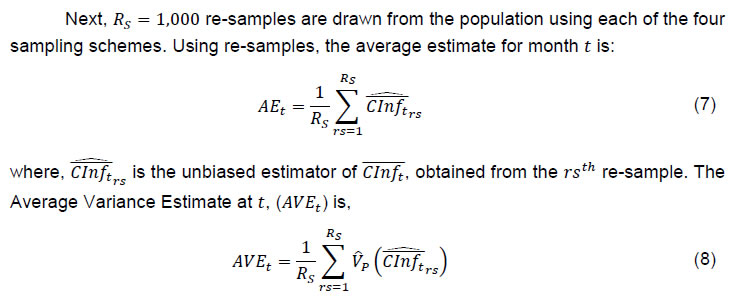

Next, it is intended to compare the households’ inflation perceptions and expectations in terms of both gap and correlation with the simulated baskets’ inflation of the survey month as well as of the month previous to the survey month (presuming households remember events of the immediate past). Table 2 shows the correlations of households’ expectations for different lags (0, 1 and 2) and leads (0 and 1) of the estimated inflation in the simulated baskets. The gap between households’ inflation expectations and estimated inflation is also tabulated. It is preferable to get high and significant correlation figures. In addition, there should not be enough evidence to support significant gap between the expectations and the estimated inflation in the simulated baskets.

The initial presumption was that if the survey expectations are close to and well-correlated with the inflation estimates obtained from the simulated baskets, then it would provide an empirical evidence to the general understanding that heterogeneity in the composition of consumption baskets is a crucial reason for the deviation of households’ inflation expectations from the official CPI-U inflation figures. From the findings of Method 1, it is understood that although the correlation figures are high and significant, the gaps with respect to the estimated inflation figures obtained from the simulated baskets, are significantly different from zero. Given this limitation of Method 1, we go on to design alternative logical methods as illustrated below.

III.2 Method 2

This method of basket simulation is based on the logic that the households while making expectations consider inflation of those items whose inflation figures are relatively higher than the other items in a particular month. Here, they do not consider their own consumption baskets at all; rather they look independently at the items that rank top with respect to the respective inflation figures. Thus, the items considered by the households are dynamic, i.e., they change over the months according to their inflation. Inflation in the CPI groups may display abrupt changes whose impact on households’ minds may be asymmetric and irrespective of the consumption weight.

A major disadvantage of Method 2 is that the consolidated indices corresponding to each of the baskets are not comparable across months or year, as the items may change. As a result, the year-on-year inflation figures do not actually represent the percentage change in a fixed basket of items.

III.3 Method 3

To overcome the above-noted limitation of Method 2, instead of computing the weighted index of the customised baskets, the inflation numbers of all the items in a basket are aggregated during each month under Method 3. This is done by calculating the following:

III.4 Method 4

This method goes a step ahead of Method 3. Here, it is presumed that households while making their inflation sentiments, not only consider those items whose inflation is among the highest in a month but also those items which they consume more frequently or in higher quantity than other items – identified by consumption weights. It is based on the understanding that if inflation in the items which are not in frequent use by most of the households rises, households will not be bothered much. Households may be bothered more about the rise in inflation of the necessary items of basic consumption. Given the skewed income distribution in India resulting in a skewed consumption pattern, this presumption seems logical.

III.5 Method 5

In this method, the consumption baskets are simulated following a procedure almost similar to the previous method. The main difference here is that, items considered for the baskets are filtered based on a threshold on the CPI inflation and a threshold on the consumption weight in each month. The thresholds are introduced here with an understanding that households remember items whose inflation outpaced more than the tolerance level and are of frequent use. These thresholds are not derived theoretically by optimisation method, but different permutations of various values are considered for performing this simulation.

IV. Numerical Illustrations to Test the Performance of the Alternative Methods

IV.1 Methods 2 and 3

The following are the steps involved in these two methods:

IV.2 Method 4

The following are the steps involved in this method:

IV.3 Method 5

The following steps are followed:

Table 3: Combinations of Consumption Weights and Inflation
Number	CW	CPIUI(in per cent)
1	0.50	4
2	0.60	4
3	0.40	5
4	0.50	5
5	0.60	5
6	0.40	6
7	0.50	6
8	0.60	6
9	0.40	7
10	0.50	7
11	0.60	7
12	‘Combined Population’, wherein 8,334 baskets are selected randomly from the first 4 populations and 8,333 baskets are selected randomly from the remaining populations, resulting in 1,00,000 baskets in this population. This is done to inject heterogeneity in the population baskets.
13

Tables 4 to 6 display correlation and gap figures for the estimates of inflation derived from baskets sampled from the population baskets simulated using Method 5, ‘Combined Population and ‘Logic Population’ as described in Table 3 above.⁹

The performance of the estimates derived from the ‘Combined Population’ is satisfactory. However, in the estimates obtained from samples drawn from the ‘Logic Population’; not only are the correlations high and significant, there is not much evidence to reject the null hypothesis of gaps equal to zero.

Thus, the results from the ‘Logic Population’ are the best in the lot of combinations studied here. These are also evident from Chart 3 below. Further, when these results are superimposed on the efficiency of the estimates measured by Average Variance Estimate (AVE), Average Relative Bias (ARB), Average Coefficient of Variation (ACV) and Actual Coverage Percentage (ACP) (Appendix), results reflect that irrespective of the sampling scheme, the ‘Logic Population’ produces inflation estimates which are found to be close, and significantly correlated with the survey-based inflation expectations.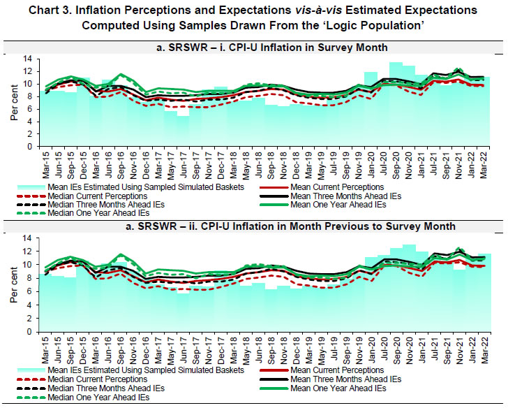

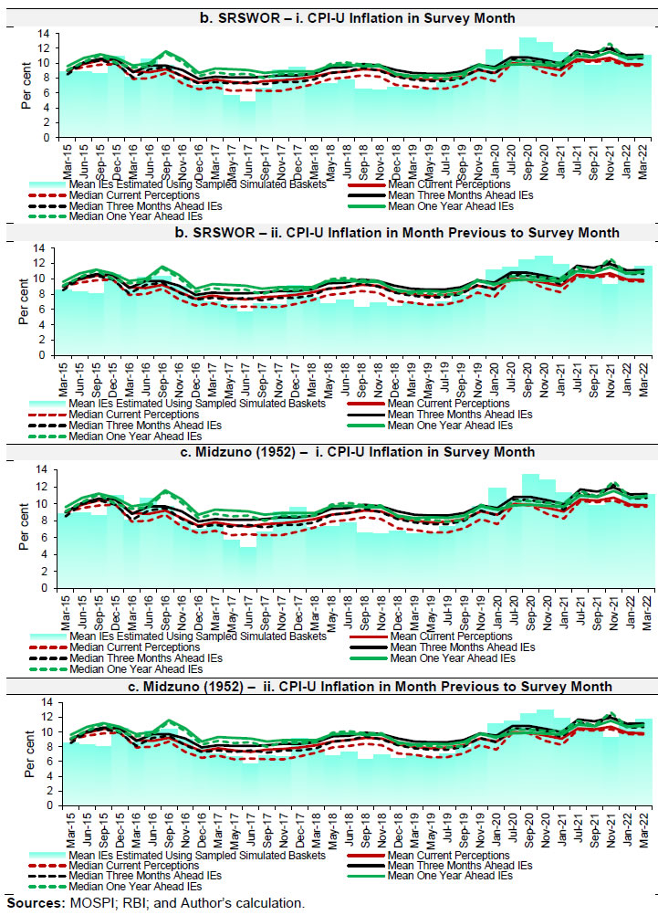Chart 4 provides an overview of select five items that rank top in inflation in the ‘Logic Population’ (list of items with consumption above the mean thresholds among items with inflation above the monthly thresholds). The major items of concern were pulses and vegetables from 2015 to 2016, vegetables, fuel and conveyance charges from 2017 to 2019 and vegetables (especially potato), refined oil and fuel during the COVID-19 pandemic.

Following are the key findings from the analysis in this section:

1. Households’ inflation expectations are largely dependent on the items that carry a high rank in inflation (more than the average inflation of items in a month) and among them, those which are consumed the most (more than the average consumption weight of items). The list of such items is dynamic and varies across months. This results in disagreement in households’ inflation expectations with respect to the official inflation figures. The results stand valid irrespective of the sampling scheme used for sampling the baskets from the simulated population baskets.

2. The inflation figures estimated using sampled baskets drawn from population consumption baskets simulated using a logic of considering items with high inflation and of regular consumption, are not only close to the survey-based expectations but also significantly correlated. Thus, a sudden rise in inflation in items of regular use can explain the deviation in households’ inflation expectations from the official inflation. These findings indicate that using a logical method for the selection of items in consumption baskets, the disagreement in survey-based expectations with respect to the official inflation can be explained.

V. Conclusions

It is generally argued in the literature that the deviation of households’ inflation expectations from the official inflation number can be the result of the diversity in households’ consumption baskets. Using data from the IESH conducted by the RBI, this paper attempts to provide empirical evidence to support this observation in the case of India. The paper takes a novel approach to verify this observation empirically. It simulates a large number of heterogeneous consumption baskets. Treating this as the population, it estimates the mean inflation in the population baskets by using sampled baskets from the simulated population. It is anticipated that the mean inflation in numerous simulated heterogeneous consumer baskets should be well-correlated and close to the survey-based expectations. Such a correlation would provide empirical support to the observation that the heterogeneity in the composition of consumption baskets is a crucial reason for the deviation of households’ inflation expectations from the official CPI-U inflation figures. This effort of finding the source(s) of disagreement in households’ inflation expectations with respect to the official inflation can assist in better understanding and using the inflationary expectations.

The paper, however, finds that although the estimated inflation figures obtained from the simulated baskets are significantly correlated with the survey-based expectations, the survey-based numbers bear significant gap with respect to the estimated inflation figures obtained from the simulated baskets.

As a result, we develop other alternative logical methods for simulating the baskets of consumption items which would provide a reason for the deviation of expectations from the CPI-U inflation. The motive is to find the best logical method for simulating the consumption baskets that would ensure that (a) the estimated inflation would deviate from the headline inflation figures; and (b) the estimated inflation would be close in number and display a high correlation with the survey-based expectations.

While most of the proposed methods do not result in satisfactory results, we obtain the desired results from the samples drawn from ‘Logic Population’ method (under Method 5 in the paper) wherein the items are considered if their respective inflation figures are more than the average inflation of items in a month and among them, those whose consumption weight is more than the average consumption weight.

The expectation estimates obtained from the ‘Logic Population’ are not only significantly correlated with the survey-based expectations but the gap between the two series is not found to be statistically significant. Irrespective of the sampling scheme used for sampling the baskets from the simulated population baskets, the ‘Logic Population’ method produces inflation estimates that are found to be close to and significantly correlated with the survey-based inflation expectation estimates.

We, therefore, conclude that households’ inflation expectations are largely dependent on the items carrying a high ranking in inflation (more than the average inflation of items in a month) and among these, the ones which carry a high weight in consumption (more than the average consumption weight of items). Evidently, the list of such items is dynamic and can vary across months.

These findings indicate that using a logical method for the selection of items in consumption baskets, the disagreement in survey-based expectations with respect to the official inflation can be explained.

^@ Purnima Shaw (pshaw@rbi.org.in) is Assistant Adviser in the Department of Statistics and Information Management (DSIM), Reserve Bank of India (RBI).

¹ Authors are thankful to Jayaraman Alur Raghavan, Sourajyoti Sardar, Pallavi Chavan, members of the DSIM Internal Advisory Group, participants of the Department of Economic and Policy Research (DEPR) Study Circle and the Editorial Board for providing useful comments which have enriched the content of this paper. The views and opinions expressed in this paper are those of the author and do not necessarily represent views of the RBI.

² State-wise analysis is not performed as CPI-inflation figures for items are unavailable for the states.

³ Here, the numbers of baskets to be simulated in the population and proportions of items to be drawn from each of the consumption subgroups of items at each step are indicative. Other values may be considered.

⁴ Item-wise CPI indices are unavailable for the months March to May 2020 due to the Covid-19 pandemic and the resulting restrictions.

⁵ The bimonthly IESH conducted by the RBI forms one of the important inputs to the bimonthly Monetary Policy. Given the limited time frame, it covers about 6,000 households (survey centre Jammu, which was added recently, is not considered for the analysis) out of the total 1,77,28,937 households (as per Census 2011) in the 18 survey centres considered for the survey. Keeping this in consideration, a small sampling fraction is considered here for the numerical illustration.

⁶ For the samples drawn from the population baskets simulated using Method 3 (to be described later in the paper), as all figures are above 16 per cent, these are not transformed into ranges.

⁷ Low fractions are considered here with the presumption that households can remember a limited number of items while making expectations.

⁸ Small percentages are considered here with a presumption that households may remember only a few items in mind while making their inflationary sentiments.

⁹ The Tables on performances of Methods 2 to 4 and of eleven combinations of CPIUI and CW for Method 5 are refrained from reporting here to conserve space, but available on request.

References

Alpanda, S., Honig, A., & Woglom, G. (2013). Extending the textbook dynamic AD-AS framework with flexible inflation expectations, optimal policy response to demand changes, and the zero-bound on the nominal interest rate. Modern Economy, 4, 145-160.

Carroll, C. (2003). Macroeconomic expectations of households and professional forecasters. The Quarterly Journal of Economics, 118(1), 269-298.

Chaudhuri, A. (2018). Survey sampling. Chapman and Hall: CRC Press, Taylor and Francis Group.

Chaudhuri, A., & Pal, S. (2002). On certain alternative mean square estimators in complex survey sampling. Journal of Statistical Planning and Inference, 104(2),363-375.

Chaudhuri, A., & Pal, S. (2022). A comprehensive textbook on sample surveys. Springer.

Ciro, J. C. G., & Zapata, J. C. A. (2019). Disagreement in inflation expectations: empirical evidence for Colombia. Applied Economics, 51(40), 4411-4424.

Ehrmann, M., Pfajfar, D., & Santoro, E. (2015). Consumers' attitudes and their inflation expectations. Finance and Economics Discussion Series 2015-015. Washington: Board of Governors of the Federal Reserve System, http://dx.doi.org/10.17016/FEDS.2015.015.

Galí, J., & Gertler, M. (1999). Inflation dynamics: a structural econometric analysis. Journal of Monetary Economics, 44, 195–222.

Man, C.H., & Peterson, M. (2019). How does inflation expectation explain the undershooting of inflation target in Japan? Time series analysis within the frame of hybrid Phillips Curve model. Jönköping University, Jönköping International Business School, Economics.

Midzuno, H. (1952). On the sampling system with probabilities proportionate to sum of sizes. Annals of the Institute of Statistical Mathematics, 3, 99–107.

Murphy, R., & Rohde, A. (2018). Rational bias in inflation expectations. Eastern Economic Journal, 44, 153–171.

Pattanaik, S., Muduli, S., & Ray, S. (2020). Inflation expectations of households: do they influence wage-price dynamics in India? Macroeconomics and Finance in Emerging Market Economies, 13(3), 244-263.

Shaw, P. (2019), Using rational expectations to predict inflation”, Reserve Bank of India Occasional Papers, 40(1), 85-104.

Singh, D. P., Mishra, A., & Shaw, P. (2022). Taking cognisance of households’ inflation expectations in India. Reserve Bank of India Working Paper Series No. 02.

Souleles, N. S. (2004). Expectations, heterogeneous forecast errors, and consumption: micro evidence from the Michigan Consumer Sentiment surveys. Journal of Money, Credit, and Banking, 36(1).

Taylor, J. B. (1982). The role of expectations in the choice of monetary policy. Monetary Policy Issues in the 1980s, Economic Symposium Conference Proceedings August 9-10, 1982, pages 47-76.

Zhao, Y. (2021). Uncertainty and disagreement of inflation expectations: evidence from household-level qualitative survey responses. Journal of Forecasting, 41(4), 810-828.

Appendix