Press Release

RBI Working Paper Series No. 06

Sourajyoti Sardar, Anirban Sanyal, Tushar B Das^@

Abstract

¹ Applying latent class analysis to unit-level data from the Consumer Confidence Survey, this paper brings out the heterogeneous impact of the first and the second wave of the COVID-19 pandemic on Indian households in terms of five parameters, namely their current perceptions and assessment of future outlook about economic conditions, employment, price level, income, and spending. There was a deterioration in the perception of consumers towards current economic conditions across all latent classes (grouped based on city, i.e., the survey centres; annual income of the households; occupation category of the respondents; and time, i.e., survey rounds relating to peak periods of the first two COVID-19 waves) during the pandemic period. There was a worsening of perception across all latent classes for current income and employment conditions as well as their future outlook.

JEL Codes: D31, E31, E37, E52, E62

Keywords: Consumer confidence, latent class analysis, heterogeneity, COVID-19, model selection, policy, economic situation

Introduction

Consumer confidence – a tachygraphic axiom for public opinions of economic situations – is a barometer of the health of the economy from the perspective of the consumers. It provides valuable information on the present economic conditions and their future direction by interacting with consumer behaviour. Macroeconomic expectations of individuals are influenced by their socioeconomic status (Das, 2017). As a result, heterogeneity in the socioeconomic conditions of individuals can create significant differential in their forecasts (Mankiw et al., 2003; Souleles, 2004; Puri and Robinson 2007; and Dominitz and Manski, 2007). Economic agents with higher income or secure employment conditions are usually more enthusiastic about future macroeconomic events. Interestingly, the heterogeneity in perception reduces considerably during economic downturns (Das, 2017).

The heterogeneity is typically associated with the differences in various socio-demographic traits of individuals. However, it may often be difficult to capture all relevant socio-demographic attributes of individuals (Hess, 2014). Hence, the literature talks about an underlying fixed personal characteristic, such as vulnerability to depression that can explain the general pessimism and poor economic choices made by individuals, ultimately leading to poor socio-economic outcomes (Puri and Robinson, 2007).

The COVID-19 pandemic has had significant repercussions on the global and the Indian economy. Anecdotal evidence suggests that the pandemic affected households differently. Using data from the Consumer Confidence Survey (CCS) of the Reserve Bank of India (RBI), this paper analyses the heterogeneity in the economic outlook across respondents during the first and the second wave of the pandemic. Given the category-wise responses on household characteristics, identification of heterogeneous classes of households becomes a challenging task. We therefore use latent class analysis (LCA) on the household characteristics to determine the class membership of responding households. The latent classes are identified separately for the pre-COVID (2019) period, the first wave of COVID (2020) and the second wave of COVID (2021). The posterior response probabilities of each latent class are analysed for each response category to unveil the heterogeneous outlook of respondents.

Policy makers collect information on consumer sentiments about the economy through consumer confidence/ sentiment/ expectation surveys. Survey of Consumers, University of Michigan; Joint Harmonised EU Programme of Business and Consumer Surveys; Fecomercio SP’s Consumer Expectation Index used by Banco Central Do Brasil, Consumer Survey, Bank Indonesia; FNB/BER Consumer Confidence Index, South Africa; Economic Conditions and Household Circumstances, Bank of Japan; Nielsen Global Survey of Consumer Confidence and Spending Intentions, Hong Kong; and Westpac-Melbourne Institute Survey of Consumer Sentiment are some of the notable examples of such surveys.

The RBI has been conducting the CCS since June 2010. Over time, the coverage of the survey has been extended; currently, the survey is conducted in 13 cities covering 5,400 households on bi-monthly basis to cater to monetary policy objectives. The CCS captures households' current perceptions (i.e., the current situation as compared to a year ago) and future expectations (i.e., one year ahead expectations), with respect to five parameters - economic condition, employment scenario, general price levels, income and spending of households.

The paper observes heterogeneity in the survey responses on general economic conditions and other parameters. LCA reveals the presence of four different latent classes among the respondents. These four classes reacted differently during the two waves of the pandemic. The optimism in current economic conditions declined during the first wave of the pandemic and turned highly pessimistic across the latent classes during the second wave. Likewise, the optimism about future economic conditions was shaded during the first wave of the pandemic, and three-fourth of the latent classes turned into negativity during the second wave.

The pessimism about current income and employment scenarios dragged the overall economic perception down, although the outlook remained positive for some of the latent classes. There was a decline in optimism in the perceptions about current spending during the first wave, which continued to be benign during the second wave. The future expectations about spending also waned across all latent classes, indicating a precautionary motive for savings among households. Price expectations were elevated during the second wave of pandemic, possibly on account of supply chain disruptions. The overall outlook on price level was inflationary.

The remaining part of the paper is organised as follows - Section II provides a review of the existing literature. Section III illustrates the data and presents the stylised facts. Section IV outlines the empirical framework, and Section V describes the empirical findings in detail. Possible economic implications are provided in Section VI, followed by concluding remarks in Section VII.

II. Literature Review

Central Banks consider household expectations about the current and future economic conditions while formulating monetary policy. The literature indicates that households adjust their expectations differently under uncertainty (Bertola et al., 2005). The empirical evidence of heterogeneous adjustments was first noticed by Lam (1991) using Panel Study of Income Dynamics (PSID) Data. He observed significant influence of liquidity constraints and market imperfections household income. Attanasio (2000) observed the role of triggers on consumers’ decisions to purchase cars from Consumer Expenditure Survey (CEX) Data.

The inherent adjustment costs, which influence household expectations about future economic conditions, are often influenced by economic uncertainty (Eberly 1994; and Hurst and Leahy, 2000). The adjustments in expectations tend to be heterogeneous among households and are driven by household characteristics. Such divergence in expectation adjustments, observed in Michigan Consumer Sentiment Survey, was classified as survey response bias, and raised questions about rationality of respondents. Indeed, rationality of households is found to share a positive but weak correlation with future expectations about income scenarios (Flavin, 1991; and Souleles, 2004). However, this hypothesis was rejected by Keane and Runkle (1990) who used the information theory to support heterogeneous response adjustments. According to the information theory, households differ in terms of information content, and they adjust their expectations gradually over a longer horizon.

Souleles (2004) observed household information set as a major factor fueling heterogeneity in expectations about future income from unit-level Michigan Survey data. In recent studies, Das et al. (2017) have highlighted that the heterogeneity in expectations is mainly due to the socio-economic characteristics of respondents. They observed that high-income and highly educated respondents were more optimistic in terms of their future expectations. Further, they found that the variation in expectation reduced during recessions, and widened during the economic upswings. The heterogeneity in response could be linked to psychological assessment by the households. Sturge-Apple et al. (2016) provided a neuro-scientific explanation behind heterogeneity in survey responses.

Studies have also analysed the heterogeneity among consumer expectations during the recent pandemic. The impact of the pandemic could be seen in many ways. There were labour market disruptions that translated into widespread income losses across countries (Khamis et al., 2021). A World Bank survey observed that the effect of COVID-19 was asymmetrically more among low education and low skilled working classes. A European Central Bank survey on consumer expectations revealed that the pandemic affected households at large but the effect was most significant for households with younger members, female members and low-income individuals Christelis et al., 2020).

Coibion et al. (2020) analysed the effect of the lockdown on income, consumption and future expectations of households in the US. They observed a 10 per cent increase in unemployment expectations and falling inflation expectations. They also observed that following uncertainty, households put on hold their large-ticket purchases of durables. Using New York Fed's Survey of Consumer Expectations, Armantier et al. (2021) observed staggered adjustment of inflation expectations. Further, they observed that the households were affected by the uncertainty caused by the pandemic, leading to wider variations in inflation-related perceptions among respondents. Similar pessimism was visible in the survey conducted by McKinsey (2021).

The effect of the pandemic and subsequent lockdowns also affected firms' pricing policies, as they were reluctant in changing prices in the face of supply chain disruptions and slump in aggregate demand. The heterogeneity in perceptions following the pandemic was also observed in survey-based studies conducted by the London School of Economics, Harvard and many other institutions. The effect lasted over a longer period, and magnitude among various classes of households. The latest round of the Survey of Consumer Expectations of the New York Fed revealed significant improvement of households’ expectations due to the financial support provided by the government (Armantier et al., 2021)².

India’s experience was not different from other countries. According to a report published by the Boston Consulting Group (BCG) in 2021, the consumption effect of the pandemic was severely felt by Indian households. They observed 10 to 20 per cent moderation of consumption demand during the pandemic, which would reach the pre-pandemic level only by 2022. Bertrand, Krishnan and Schofield (2020) analysed the Consumer Pyramids Data from CMIE and observed significant loss of income in India during the pandemic. Using the same survey, Sanyal et al. (2021) identified the heterogeneous impact of the lockdown on income and consumption levels across household categories. They also found differential severity of the impact over the first four months of lockdown on household income and consumption. Combining the heterogeneity of households’ expectations and recent experience of the lockdown in India, it is argued that the households altered their expectations on economic conditions differently based on their socio-economic status and other characteristics.

LCA, the methodology used in this paper, was first introduced by Lazarsfeld (1950). Later the framework was revised and enhanced by Clogg (1981;1995), Hagenaars (1990), Vermunt (1997), and Nylund-Gibson and Choi (2018). LCA is extensively used in social sciences. They are also used to validate data consistency in survey responses. Kumar et al. (2012) analyse the data consistency of Consumer Confidence Survey data using latent class analysis.

LCA falls under the broad class of mixture modeling techniques. Mixture modeling is extensively used in social and behavioral sciences to detect heterogeneity in the survey responses. Bucholz et al. (2000) analysed personality disorder using LCA models. Some notable examples where LCA was used for analysing behavioral data were eating disorder analysis (Keel, 2004), attention deficiency analysis (Rasmussen et al., 2002), and comorbidity study (Sullivan and Kessler, 1998).

Though LCA models were earlier used for analysing discrete data, their application was extended to continuous variables by Lubke and Muthén (2005), Muthén (2006), Muthén and Asparouhov (2006) and Muthén, Asparouhov, and Rebollo (2006). LCA was also used in longitudinal studies (Verbeke, Molenberghs, 2000), measurement error (Carroll et al., 2006), survival analysis (Hougaard, 2000), and market segmentation (Wedel and Kamakura, 2000).

The advantage of LCA is its distribution-free assumptions of indicators with assumption of local independence. However, the local independence assumption can be relaxed as proposed by Sinclair and Gastwirth (1996); Reboussin et al. (2008); and Bertrand and Hafner (2011).

In this context, the contribution of our paper to the literature can be understood in three major ways: first, the paper highlights possible heterogeneity in household responses about the current perceptions as well as future expectations. Secondly, it analyses the impact of COVID-19 on the response heterogeneity using households’ expectations data. Finally, the paper uses LCA to unveil the latent classes from unit level households’ expectations data. LCA is used for the pre-pandemic and pandemic responses to estimate latent classes, and check the rationality of responses using posterior probability estimates.

III. Data and Stylised Facts

The Consumer Confidence Survey is a useful source of information on consumer perceptions and expectations about various macroeconomic parameters. These perceptions indicate consumers’ confidence in the economy. The Survey also offers detailed information on socio-economic and demographic attributes of responding households.

As mentioned earlier, the RBI captures households' current perception as compared to a year ago, and their expectations a year-ahead for five macroeconomic parameters – general economic condition, employment scenario, general price level (and rate of change), income and spending of households (Chart 1).

The qualitative responses for each of the parameters are obtained on a three-point scale – improved/increased (current scenario) or will increase (future scenario); remain same (or will remain same) and worsened/ decreased (will decrease). The RBI further furnishes two consumer confidence indices – current situation index (CSI) and future expectation index (FEI) – based on the current perceptions and future expectations of the households respectively, on these five parameters.

Over time, the coverage of this Survey has been expanded; as of February 2022, the survey is conducted in 13 cities covering 5,400 households. Though started with a quarterly frequency, this survey is currently conducted on a bi-monthly basis to align it with the monetary policy timeline. Respondents are selected using a random sampling method.

For this paper, the respondent-level data of CCS has been used, which is publicly available in RBI’s Database on Indian Economy. May and July rounds for 2019, 2020, and 2021 have been used in this paper. Data for 2019 are used to construct the model as well as find out the appropriate number of classes which can support the model best. The same model is then applied to the data for 2020 and 2021 to examine how these classes reacted during the first and the second wave of the pandemic.

With respect to the COVID-19 timeline in India, the first wave, which was between April to November 2020, lasted longer than the second wave in 2021. Within the first phase, a nation-wide lockdown was imposed during April - May 2020, and the unlock period started from June 2020 and stretched up to November 2020. Therefore, the hardships suffered by the households were mostly during April – July 2020.

The second wave of the pandemic, well-known for the spread of Delta variant, started during the middle of March 2021 and its severity lasted up to the middle of July 2021, during which regional lockdowns were imposed. No major variations were observed in the demographic characteristics of respondents between the data for 2019, 2020 and 2021 (Table 1).

While macroeconomic conditions are explained well by the aggregated data, respondent-level data offers more insights (Lahiri, 2016). Household perceptions and expectations on economic indicators exhibit considerable heterogeneity. Expectations can be influenced by behavioural aspects, media, complexity of the macroeconomic parameter, understanding of both surveyors and respondents, etc.

The literature indicates that demographic factors play a crucial role in influencing household expectations (Dow, 2016). Household expectations on economic parameters are multi-dimensional in nature and depend on interactions of several demographic and socio-economic factors.

To understand the heterogeneity among household perceptions and expectations owing to demographic factors during the pandemic and pre-pandemic period, the combined CSI and FEI are plotted alongside the demography-specific CSI and FEI (Chart 2). Initially, households thought the first wave of the pandemic was transitory. Therefore, the extent of pessimism was lower in FEI as compared to CSI. Interestingly, a persistence of the pandemic reinforced the cynicism among households and a notable divergence between the FEI and CSI was observed thereafter.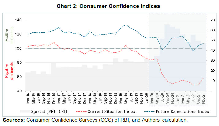

CSI and FEI varied across the socio-economic brackets indicating heterogeneity and suggesting that the pandemic affected these groups differently. The pandemic affected the low-income groups severely as compared to high-income groups. Besides, pessimism among the high-income groups bottomed out earlier than the low-income groups (Chart 3). A similar pattern was observed in future expectations. The outlook of the high-income groups was more optimistic during the recovery phase than low-income groups. This underlined heterogeneity in forward-looking economic assessment among respondents.

Similarly, households with stable income from the fixed employment were certainly less pessimistic than the self-employed or daily labourers. Retired respondents showed less pessimism possibly owing to their security of a steady pension income. Outlook of the self-employed/ business category, though improved after the first wave, weakened more rapidly during the second wave (Chart 4).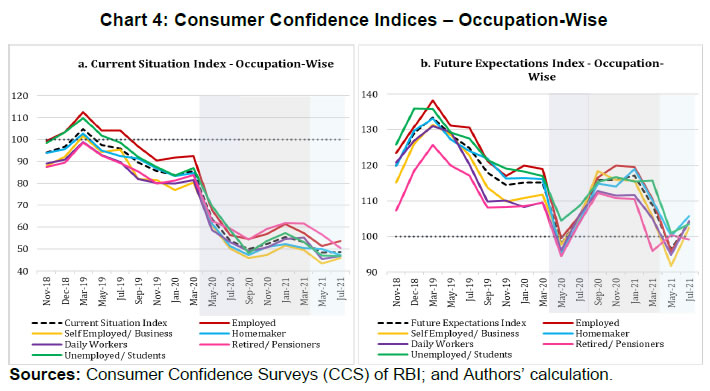

The perception also varied across cities covered in the Survey. We have shown Tier-I and Tier-II cities in Chart 5 to maintain the clarity in presentation.³ Negativity in confidence was lower in Tier-II cities than Tier-I cities for both current perception and future outlook. However, the pessimism was much less with regard to the future outlook than the current situation in Tier-II cities. Such variations were expected considering that cities experienced lockdowns at different points of time. The administrative measures to restrict movements differed not just across cities but also across the various waves of the pandemic.

Such heterogeneous distribution of responses underlined the possibility of latent classes owing to respondents’ characteristics and spatial locations. Such latent classes cannot be observed directly but are estimated from the unit-level data, as attempted in this paper.

IV. Methodological Framework

Latent class analysis has many advantages compared to conventional clustering techniques. The choice of classification in LCA is less arbitrary due to the underlying statistical model, and hence, offers various assiduous statistical tests to assess model fitness. It further lays out the conditions to make decisions about the suitable number of clusters. The probabilistic nature of cluster membership in latent class cluster analysis leads to less biased estimations of class-specific means, as each case only contributes to this mean weighted by its class membership probability (Karnowski, 2017).

The model can be estimated using a simplex algorithm, proposed by Dayton and Macready (1988). However, the standard error of estimates cannot be obtained using this approach. Following Bandeen-Roche et al. (1997), the model is estimated using the EM algorithm. The link function is assumed to be logistic in nature. Starting with an initial guess about the class probabilities and covariate effects, the estimation approach calculates the posterior class probabilities from the initial guess and then, it updates the class probabilities and regression coefficients by maximising the log likelihood function.

LCA involves various steps involving variable choice, class numbers and estimation before reaching the best-suited model for the data. Hence, a step-wise approach has been followed to determine the optimal choice of model.

Step 1: Identify grouping variables.

Step 2: Select the best model using suitable grouping variables.

Step 3: Select the optimal number of classes.

Step 4: Estimate the model parameters.

Step 5: Estimate posterior class probabilities.

Grouping of variables is used to identify the latent classes, following Biemer and Winsen (2002). Hui and Walter (1980) first suggested the grouping of respondents’ characteristics⁵ to improve the goodness of fit and reduce unexplained leftover heterogeneity. The underlying assumption behind grouping variables is that the grouping variable should be highly correlated with the latent classes. In this paper, different grouping variables are used to carve out the best of the breed model.

Models -

f1: Y ~ Time

f2: Y ~ Income + Time

f3: Y ~ Occupation + Time

f4: Y ~ City + Time

f5: Y ~ Income + City + Time

f6: Y ~ Occupation + City + Time

f7: Y ~ Income + Occupation + Time

f8: Y ~ City + Income + Occupation + Time

where, Y is the survey response across various categories. Here, Y = (A, B, C, D, E, F, K, L, M, N)⁶ and the variables imply the following:

'A' - perception on general economic situation - compared to one year ago;

'B' - outlook on general economic situation - one year ahead;

'C' - perception on household income - compared to one year ago;

'D' - outlook on household income - one year ahead;

'E' - perception on overall household spending - compared to one year ago;

'F' - outlook on overall household spending - one year ahead;

'K' - perception on employment scenario - compared to one year ago;

'L' - outlook on employment scenario - one year ahead;

'M' - perception on general prices - compared to one year ago;

'N' - outlook on general prices - one year ahead; and

time, income, occupation, and city are the grouping variables or covariates.

Among these specifications, the best model is selected using the goodness-of-fit measures. Currently, there is no consensus among researchers about the optimal goodness-of-fit criteria. The likelihood ratio test is not suitable for detecting optimal models due to lack of regularity conditions. Often, mixture modelling uses information criteria (AIC, BIC) along with subjective assessment to choose the best model. Lanza et al. (2002) proposed BIC as the optimal information criteria for the model selection. Yang (2006) proposed adjusted BIC as optimal information criteria.

In this paper, BIC is used to determine the optimal grouping variables. Beyond the information criteria, Wang (2017) proposed another criterion based on entropy⁷ measures for running model diagnostics. Entropy measures the goodness-of-fit in terms of class representations. Generally, a higher value of entropy is acceptable. Celeux and Soromenho (1996) suggested using entropy measures of 1 (at least higher than 0.8) for accepting a good model. However, the threshold value of entropy-based measures is not available. In this paper, an entropy estimate of at least 0.6 is used for identifying the optimal model.

After the grouping variables are decided, the optimal number of latent classes are analysed, given the responses. As the number of classes increases, the parameter space expands exponentially. Hence, it is decided to restrict the analysis with the number of latent classes as 2, 3 and 4.⁸ Further, the power of latent class models depends heavily on the sample size. Hence a pertinent question is: what is the optimal sample size to get a reliable estimate? While a higher number of data points is the obvious choice, Nylund - Gibson and Choi (2018) suggested using at least 300 observations to get consistent estimates of the covariates. Often, researchers use Monte Carlo simulations to determine optimal sample size. In this paper, large sample sizes (more than suggested) are used to estimate the model. In that sense, the model parameters are expected to be stable, and the estimation process is likely to converge.

Next, the posterior class probabilities are used across different outcome variables (i.e., income, price, economic conditions, etc.) to map the characteristics of the latent classes with response probabilities. Using these steps, the latent class models are estimated using unit level survey responses for pre-pandemic and pandemic periods (the first and the second wave). The latent classes and posterior probability estimates are available for each of these time spans.

In this paper, the latent class compositions are compared for these three episodes. The pandemic effect is reflected from the posterior probabilities of latent classes. The empirical findings are summarised by looking at the posterior probability estimates across different outcome variables and commenting on the respondents’ rationality in each outcome variable in each episode.

A series of robustness checks are carried out in each step of the process. The first round of checks was carried out using different combinations of grouping variables and estimating the information criteria for each choice of grouping variables. The choice of grouping variables was found to be robust among those choices. Besides, the stability of the grouping variable selection along with the choice of classes were carried out using bootstrapping. Using 80 per cent of the unit-level responses from the pre-pandemic period, the model selection criteria is analysed for each bootstrap round. Class-4 model estimates were found to be stable compared to Class-5 model results. The sensitivity of the latent class estimates was further checked using bootstrapping. An application named poLCA⁹ from the R software is used for the analytical work.

V. Empirical Findings

V.1 Model Selection

As indicated earlier, the grouping variables are determined in the empirical analysis. The competing models (f1-f8) are tested to identify the suitable grouping variables using data for May and July 2019.¹⁰ The models are validated using information criteria (AIC, cAIC, BIC and aBIC) and Chi-square. The AIC and cAIC estimates evaluate f8 (i.e., grouping variables city, income, occupation and time) as the best model. Though model f4 also exhibits better AIC estimates for class-2 and class-3 models, f8 is deemed as a suitable grouping model given the unit-level responses due to better in-sample fit criteria for higher class models (Table 2).

Additionally, the grouping variable selections are tested using BIC criteria and Chi-square estimates. The paper observes a similar selection of grouping variables using BIC, aBIC and Chi-Square estimates (Table 3).

V.2 Selection of Appropriate Number of Classes

We use city, income, occupation and time as grouping variables and the model is estimated once again to determine the optimal number of classes from the survey responses using information criteria and entropy measures. Table 4 represents estimates of AIC, BIC and entropy estimates for each class model.¹¹

The entropy estimates are greater than 0.7 for all classes of models which implies that the models are acceptable under the generally acceptable threshold of 0.6. Further, the BIC criteria indicate that Class-4 and Class-5 models are suitable candidate models for capturing the respondents’ heterogeneity in responses, whereas the BIC of Class-3 model is sufficiently higher than Class-4 model. Also, the BIC estimate of the Class-4 model is closer to the Class-5 model. Hence, the final choice of model is restricted to the Class-4 model with the choice of grouping variables.

Further, the same procedure is repeated using May and July responses for 2020 and 2021, corresponding with the peak of the pandemic. Class-4 appears to be the optimal choice for both the episodes (Chart 6).

V.3 Latent Class Characteristics

Next, the latent classes are characterised using the estimated coefficients of the income and occupation levels. Table 5 represents the coefficient estimates of each income and occupation category.¹²

Covariates are included in the latent class regression model through their effects on the priors P_r. In the basic latent class model, it is assumed that every individual has the same prior probabilities of latent class membership. The latent class regression model, in contrast, allows individuals' priors to vary depending upon their observed covariates.

It must be pointed here that these coefficients are reported as odds ratio with respect to the reference class (i.e., odds with respect to the reference class). The reference class represents equal representation from all income and occupation classes. The first coefficient value of 0.63 (class-1 in pre-pandemic) indicates odds of 0.63 of respondents having income between 1 lakh to 3 lakh to belong to class-1 compared to Class-4 (reference class). On the contrary, respondents of this income group are almost equally likely to be in Class-2 and Class-3 with respect to the reference class.

Comparing the coefficient values of all income classes in Class-1, respondents with Rs.1 lakh to Rs.3 lakh of income have a greater likelihood to belong to Class-1 among all income categories. Similar arguments can be drawn with respect to occupation categories also. Homemakers and unemployed/ students have equal odds to be part of latent Class-1, whereas latent Class-2 has similar odds of having employed, homemakers and unemployed. Moving on to the odds ratio estimates from the first wave of COVID-19, the income group of Rs.1 lakh to Rs.3 lakh and Rs.5 lakh and more have similar odds of being in Class-1 as compared to the reference class.

The likelihood of Class-2 membership is greater for medium income (i.e., Rs.3 lakh to Rs.5 lakh) and high income (i.e., Rs.5 lakh and more) groups. Among the occupational groups, self-employed, and business owners have greater likelihood to be part of Class-1 whereas retired/ pensioners are likely to be a part of Class-2. Lastly, unemployed/ students have greater odds of being in Class-3 during the first wave of pandemic.

With regard to the second wave, the odds of each income and occupational class started aligning to balanced representation across all latent classes. While low-income respondents had a greater representation in Class-1 during pre-pandemic period, the odds improved for high-income respondents of being in Class-1 during the second wave of the pandemic. However, the overall comparison of classes across these three episodes should not be done as the benchmark class differs across these time periods.

The “estimated class population shares” section of the output provides the estimated proportions corresponding to the share of observations belonging to each latent class (Linzer and Lewis, 2011). Therefore, in the case of the Class-4 model, the share of observations is estimated to be 21.43 per cent in latent Class 1, 28.36 per cent in latent Class 2, 20.54 per cent in latent Class 3 and 29.67 per cent in latent Class 4 (Table 6).

V.4 Conditional Item Response Probabilities/Posterior Response Probabilities

The conditional item response probabilities or posterior response probabilities are calculated using equation (4), by outcome variable, for each class. This output shows the probabilities of respondents in each latent class providing an optimistic (choice of option equal to increased/ improved/ will increase), neutral (choice of option equal to remained same/ will remain same) or pessimistic (choice of option equal to decreased/ worsened/ will decrease) response to the indicator variable in question. These choices are represented as Pr(1), Pr(2) and Pr(3), respectively. For example, the conditional item response probabilities for the ‘current general economic condition’ variable produced in Class-4 model for three distinct time frames i.e., pre-pandemic, the first wave, and the second wave of the pandemic are given in Table 7. For instance, the probability estimate of 0.6832 represents posterior probability of optimism for Class 1 respondents. The detailed results are given in the Annex.

The optimism about general economic conditions (before the pandemic) wore off rapidly during the first wave (May and July 2020) and continued to remain depressed during the second wave (May and July 2021). The first shock of the pandemic was less anticipated. The optimistic respondents from pre-pandemic time, adjusted their outlook to the worsening economic conditions. The impact of the second wave intensified the pessimism even further. Here, it must be remembered that the heterogeneous classes are differently estimated for each time period and hence are not exactly comparable in nature.

Contrary to their perception about current economic conditions, the outlook of the consumers about the economic conditions remained mostly positive during the first wave of COVID-19. The economic outlook remained upbeat across three of the four latent classes during the first wave. The optimism was revised downwards with the spread of the Delta variant (Table 7).

The conditional item response probabilities of the general economic situation for current perception and one year ahead outlook have already been explained. Now, a pictorial representation (Chart 7) of the Class-4 model combining all the survey parameters across three different time frames of our interest will provide a holistic understanding how the representation of these classes changed during the first and the second wave of the pandemic. It has been described as ‘posterior net response’ (PNR) by the authors.

V.5 Posterior Net Response

The posterior perception of latent classes about household income, spending, employment and general prices are analysed next. Using the posterior estimates of each latent class under each response category, the posterior net response (PNR) is defined by netting out the posterior probability of negative responses from posterior probability of positive response¹⁴, i.e., net pessimism or net optimism depending on its sign, which varies between (-1) to (+1). For instance, if the posterior probability of improvement in household income is 0.7 and posterior probability of deterioration of household income is 0.1 (i.e., probability of income remains same being 0.2), the net response of perception of household income will be 0.7 - 0.1 = 0.6. One can, therefore, interpret positive PNR as upbeat/ optimism about the response category.

With this background, the PNR for perception of current and outlook about future income across the four latent classes are derived.

The confidence among the consumers regarding the general economic situation weakened during the first wave of pandemic and worsened further during the second wave (Table 7 and Chart 8). On the other hand, the general economic outlook, though weakened a bit during the first wave, its weakening intensified further during the second wave.

The pessimism in household income intensified during the first wave of pandemic and remained at almost similar level during the second wave. The upbeat about future income from pre-pandemic time also ebbed across classes. However, unlike the current income scenario, some latent classes maintained their positive outlook about improvement in future income during the first wave. The optimism marginalised across the majority of latent classes during the second wave (Refer to Chart 9).

The perception about current household spending changed drastically during May – July, 2020 compared to the corresponding period in 2019. The unprecedented impact of the pandemic during its first wave restricted spending patterns across latent classes. As households were unprepared at the time of the first wave, the spending cut along with reduced income perception, plausibly indicated precautionary savings.

During the second wave, perception on spending somewhat improved for most classes. The precautionary saving by cutting spending was an optimal strategy for latent Class 3 (Chart 10).

Perception about employment conditions deteriorated during the first and the second wave as compared to the pre-pandemic period. The PNR remained negative across all latent classes during May-July 2020 and 2021. The marginal optimism about improvement in employment conditions turned into severe pessimism during the first wave period as lockdown restricted economic activities across places resulting in job losses.

The pessimism about employment perception persisted during the second wave. However, unlike the current perception, the outlook about future employment conditions remained mixed across latent classes during the first wave of the pandemic. Majority of latent classes anticipated improvement in employment conditions, indicating that the respondents viewed the pandemic to be transitory. However, during the second wave, most latent classes revised their future outlook downwards. This revision was a reflection that respondents began to realise that the pandemic was here to stay (Chart 11).

Lastly, we analyse the PNR about current and future price levels. Here, PNR is defined by netting out the posterior probability of positive responses from posterior probability of negative response as increase in prices is inflationary and considered as a negative sentiment. Besides, a negative net response about price level indicates inflationary outlook and hence is a concern for the monetary policy.

Households' inflation expectations indicate whether the long-term expectations are well-anchored to the inflation target. The perception about price level remained net negative before the pandemic. The perception about current price level did not change much during the first wave of pandemic but the inflationary perception from current price level elevated across all latent classes during the second wave. The outlook about future price level, however, remained mixed across latent classes during the first and the second wave. The change in the respondents’ perception about the current price level during the second wave of the pandemic and moderation of the future spending demand outlook mirror the effect of supply chain bottlenecks (Chart 12).

VI. Economic Implications

This pandemic was a once-in-a-lifetime event and took the households by surprise. During abnormal times, consumers’ perception becomes pessimistic regardless of their socioeconomic status. Multiple waves made consumers even more pessimistic leaving little room for policy to turn around such sentiments.

The paper observed heterogeneity in respondents’ assessment and expectations about the five macroeconomic parameters. Households from the optimistic latent classes had positive posterior net response (PNR) about the economic conditions, employment and income scenario during the pre-pandemic period. Latent Class-1 and 4 were optimistic about their assessment of overall economic conditions, whereas, Class-2 and 3 respondents had a pessimistic assessment during the pre-pandemic period (refer to first part of Table 8). Latent Class-2 represented homemakers with lower income level, whereas Class-3 represented unemployed/ students coming from lower tail of income distribution.

During the first wave, all latent classes experienced weakening in the current economic activities. Class-1 and 2 respondents showed greater pessimism in current economic assessment, while Class-3 and 4 respondents were less pessimistic. Class-1 mainly comprised homemakers and unemployed/ students from all income groups whereas Class-2 had pensioners/ retired respondents from all income groups. These respondents expressed concerns about deterioration in employment conditions and real income loss against the backdrop of rising price levels. Between these two classes, pensioners/ retired respondents possibly resorted to spending cuts to cope with the economic downturn. On the other hand, Class-3 respondents were salaried and students/ unemployed persons belonging to high-income brackets. These respondents expected less income employment conditions (refer to the middle part of Table 8).

Lastly, all latent classes expected an economic downturn during the second wave of the pandemic. However, unlike the first wave, all classes started aligning their assessment about current economic conditions during this wave. Class-2 and 3 demonstrated the worst slowdown in current economic conditions, whereas Class-1 and 4 respondents were relatively optimistic.

The estimates of odds ratio from this episode revealed that self-employed/ business owners at the lowest income level had a greater likelihood of being in Class-2. Class-3 composed of self-employed/ business owners, homemakers, and unemployed/ students with relatively higher income levels. Class-1 respondents are self-employed/ business owners with middle-income and higher-income levels.

The larger pessimism of Class-2 was driven by severe contraction in income and employment conditions with an increased spending and higher inflation assessment. Class-3 respondents expected greater income loss and loss of employment, but they were less inclined to spending cuts contrary to Class-2 respondents. The less pessimistic respondents from Class-1 and 4 expected lower income loss and relatively better employment conditions. All four latent classes expressed concerns about elevated price levels (Refer to last part of Table 8).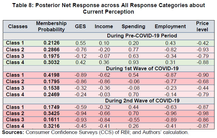

In general, households were seen to be optimistic about the future, despite a little distress in the present conditions. During the pre-pandemic period, the optimism about outlook was fueled by better employment and income conditions in the future. Most optimistic households, i.e., Class-1 and 4 were upbeat about the future economic conditions supported by better income, employment and spending. Hence, their outlook about price expectations was likely to have been driven both by the demand and cost factors (Refer to first part of Table 9).

As the pandemic started, around 42 per cent of households classified under Class-1 (comprising homemakers and unemployed/ students) became pessimistic about economic conditions mostly due to higher price expectations, and increased spending coupled with low income and weak employment conditions. The other latent classes remained upbeat about future economic recovery.

Class-2 and 4 respondents expected recovery in income and employment conditions to a greater extent. Lastly, Class-3 respondents demonstrated a moderate recovery in overall economic conditions fueled by improvement in income and employment along with maintaining their spending pattern. The price level outlook remained high for Class-1 and 4, whereas Class 2 and 3 expected relatively lower price rise (Refer to middle part of Table 9).

During the second wave, the expectations on economic recovery faded across all latent classes; 70 per cent of households turned pessimistic. Among these latent classes, Class-1 respondents displayed no improvement in overall economic conditions, and they remained indecisive about any improvement in employment conditions with elevated levels of future spending. Class-2 respondents faced greater threats from future employment conditions and higher spending levels with no significant increase in income level. Class-3 expected worsening of employment conditions with no income growth. Unlike the other three classes, Class-4 remained optimistic about future economic recovery, fueled by their outlook on better employment and better income with an increase in spending. The future price level remained a source of concern for all latent classes (Refer to last part of Table 9).

The gradual alignment of economic assessment and outlook across various latent classes suggested learning by households as the pandemic progressed. According to the concept of bounded rationality, economic agents use learning models for their expectations and hence, they insure themselves from future covariate shocks by cutting consumption spending and focusing on greater saving.

As the pandemic increased uncertainty about the future economic recovery, consumers resorted to spending cuts. In this situation, a sound forward guidance with a promise of a low yield environment - which also followed RBI's policy action in this matter – was expected to lower precautionary savings and enhance consumption driven growth (Acharya et al., 2020). Precautionary saving may lower the inflationary risk, providing better policy space for the central bank. However, elevated uncertainty can dampen the effectiveness of central bank’s forward guidance, leading to forward guidance puzzle (Negro et al., 2015).

Moreover, respondents’ perception about the duration of the pandemic also played a role in deciding their response. Following the Delta variant, consumers began to consider the pandemic shock to be a persistent one. Therefore, consumers maintained their stance on consumption patterns, and hence, timely forward guidance from the central bank towards a gradual and calibrated normalisation spurred economic recovery. Further, lower cost of borrowings was expected to spur investments and employment. Nonetheless, downside risks remained from supply chain bottlenecks. Households’ perception about current price level elevated inflation risk during the second wave. Higher inflation expectations and benign consumption demand can affect economic recovery. Coordinated and calibrated fiscal and monetary policy measures can help in achieving economic recovery at a faster pace.

VII. Conclusion

Forward-looking surveys provide important insights on households’ expectations about the future, and hence are useful to policy. However, these expectations, being influenced by the information available to individual households, are often found to be heterogeneous in nature.

In this paper, the hidden heterogeneity in household responses is unearthed using LCA. The paper classifies households into four latent classes using city, i.e., the survey centres; annual income of the households; occupation category of the respondents; and time, (i.e., survey rounds relating to peak periods of the first two COVID-19 waves), as grouping variables. Using these classes, the paper analyses the response pattern on overall economic situation, income, spending, employment, and general price level.

The perception about current economic conditions remained pessimistic whereas the outlook remained relatively upbeat across latent classes. The current income perception deteriorated across all latent classes, though, outlook about household income remained buoyant for some latent classes. The spending perception was influenced by generic price pressures and precautionary savings. The spending perception improved during the second wave of the pandemic but remained subdued compared to the pre-pandemic period. The outlook on future spending was similar.

The employment situation worsened over the first and second waves. The outlook about future employment remained positive for some latent classes during the first wave but moved to the pessimistic territory during the second wave. Lastly, the perception about prices suggested higher inflation expectations during the second wave, and for the year-ahead outlook.

^@ Sourajyoti Sardar and Anirban Sanyal are Assistant Advisers, Department of Statistics and Information Management, Reserve Bank of India (ssardar@rbi.org.in; asanyal@rbi.org.in). Tushar B Das is Director, Department of Statistics and Information Management, Reserve Bank of India (tbdas@rbi.org.in).

¹ The authors are thankful to Ravi Shankar, A R Jayaraman, Purnima Shaw, Ranjeeta Mishra, and seminar participants at the DEPR Study Circle. We are also grateful to Priyanka Upreti, DRG, DEPR. We acknowledge her help in revision of this paper. This paper has also benefitted from the comments of an anonymous external reviewer and authors place on record their sincere thanks for the same. However, we alone are responsible for any errors that may have remained in the paper. The views expressed in the paper are those of the authors and do not necessarily represent those of the institutions to which they belong.

² See https://libertystreeteconomics.newyorkfed.org/2020/08/the-disproportionate-effects-of-covid-19-on-households-with-children/

³ Ties 1 cities are Ahmedabad, Bengaluru, Chennai, Delhi, Hyderabad, Kolkata, and Mumbai; Ties 2 cities are Bhopal, Guwahati, Jaipur, Lucknow, Patna, and Thiruvananthapuram.

⁴ In case of continuous density, the model is called latent profile model.

⁵ Grouping variables and covariates are used interchangeably in this paper.

⁶ The other response variables are excluded due to inconsistency in responses observed by Kumar, Husain and Mukherjee (2012).

⁸ The paper also considers 5 latent classes. However, the estimates lack robustness due to data limitations.

⁹ The estimation of latent class models and latent class regression models in R (see Linger and Lewis, 2011; R Development Core Team, 2010) is based on this package.

¹⁰ The seasonal pattern in the aggregate response data is checked and the statistical tests do not find any significant seasonality in the response pattern.

¹¹ The information criteria estimates are used for selecting the model. LCA models are estimated iteratively for the determining optimal number of classes. The model fit estimates (coefficients and information criteria estimates) vary in each iteration due to the EM algorithm used for estimating the model and changes in the benchmark class (Nylund et. al. (2007)). However, the f8 model appears to be the robust model selection over different iterations of estimations and hence, f8 is considered the final model for the analysis. Further, the robustness of class selection was confirmed using bootstrap estimates of information criteria for 1000 iterations.

¹² Here, the spatial coefficients are not included to center the discussion on the income and occupation categories. Separate tables of coefficient estimates are provided in Appendix-I for completeness.

¹³ The above mathematical derivation is directly taken from the ';poLCA: Polytomous Variable Latent Class Analysis - Version 1.4'; authored by Drew A. Linzer and Jeffrey Lewis.

¹⁴ Here, the net response is not weighted as the posterior probabilities can be treated as perception of a representative household in each latent class. Hence, the posterior net response should be viewed as a net response of the representative household, rather than the response of all households belonging to the latent class.

References

Acharya, S., & Dogra, K. (2020). Understanding HANK: Insights from a PRANK. Econometrica, 88(3), 1113-1158.

Agresti, A., & Min, Y. (2002). Unconditional small‐sample confidence intervals for the odds ratio. Biostatistics, 3(3), 379-386.

Attanasio, O. P. (2000). Consumer durables and inertial behaviour: Estimation and aggregation of (S, s) rules for automobile purchases. The Review of Economic Studies, 67(4), 667-696.

Bertola, G., Guiso, L., & Pistaferri, L. (2005). Uncertainty and consumer durables adjustment. The Review of Economic Studies, 72(4), 973-1007.

Bertrand, A. M., & Hafner, C. M. (2014). On heterogeneous latent class models with applications to the analysis of rating scores. Computational Statistics, 29(1), 307-330.

Biemer, P. P., & Wiesen, C. (2002). Measurement error evaluation of self‐reported drug use: a latent class analysis of the US National Household Survey on Drug Abuse. Journal of the Royal Statistical Society: Series A (Statistics in Society), 165(1), 97-119.

Bucholz, K. K., Hesselbrock, V. M., Heath, A. C., Kramer, J. R., & Schuckit, M. A. (2000). A latent class analysis of antisocial personality disorder symptom data from a multi‐centre family study of alcoholism. Addiction, 95(4), 553-567.

Carroll, C. D., & Samwick, A. A. (1998). How important is precautionary saving?. Review of Economics and statistics, 80(3), 410-419.

Carroll, R. J., Ruppert, D., Stefanski, L. A., & Crainiceanu, C. M. (2006). Measurement error in nonlinear models: a modern perspective. Chapman and Hall/CRC.

Celeux, G., & Soromenho, G. (1996). An entropy criterion for assessing the number of clusters in a mixture model. Journal of classification, 13(2), 195-212.

Clogg, C. C. (1981). New developments in latent structure analysis. Factor analysis and measurement in sociological research.

Clogg, C. C. (1995). Latent class models. In Handbook of statistical modeling for the social and behavioral sciences (pp. 311-359). Springer, Boston, MA.

D'Amico, S., & King, T. B. (2015). What does anticipated monetary policy do?.

Das, A., Lahiri, K., & Zhao, Y. (2019). Inflation expectations in India: Learning from household tendency surveys. International Journal of Forecasting, 35(3), 980-993.

Dominitz, J., & Manski, C. F. (1997). Using expectations data to study subjective income expectations. Journal of the American statistical Association, 92(439), 855-867.

Dominitz, J., & Manski, C. F. (2007). Expected equity returns and portfolio choice: Evidence from the Health and Retirement Study. Journal of the European Economic Association, 5(2-3), 369-379.

Dow Jr, J. P. (2016). Demographic factors affecting macroeconomic expectations. Southwestern Economic Review, 43, 87-101.

Eberly, J. C. (1994). Adjustment of consumers' durables stocks: Evidence from automobile purchases. Journal of political Economy, 102(3), 403-436.

Flavin, M. (1991). The joint consumption/asset demand decision: a case study in robust estimation.

Foote, C., Hurst, E., & Leahy, J. (2000). Testing the (S, s) Model. American Economic Review, 90(2), 116-119.

Gollier, C., & Pratt, J. W. (1996). Risk vulnerability and the tempering effect of background risk. Econometrica: Journal of the Econometric Society, 1109-1123.

Hagenaars, J. A. (1998). Categorical causal modeling: Latent class analysis and directed log-linear models with latent variables. Sociological Methods & Research, 26(4), 436-486.

Hess, S. (2014). Latent class structures: taste heterogeneity and beyond. In Handbook of choice modelling. Edward Elgar Publishing.

Hougaard, P., & Hougaard, P. (2000). Analysis of multivariate survival data (Vol. 564). New York: Springer.

Hui, S. L., & Walter, S. D. (1980). Estimating the error rates of diagnostic tests. Biometrics, 167-171.

Karnowski, V. (2017). Latent class analysis. The international encyclopedia of communication research methods, 1-10.

Keane, M. P., & Runkle, D. E. (1990). Testing the rationality of price forecasts: New evidence from panel data. The American Economic Review, 714-735.

Keel, P. K., Fichter, M., Quadflieg, N., Bulik, C. M., Baxter, M. G., Thornton, L., Halmi, K.A., Kaplan, A.S., Strober, M., Woodside, D.B. and Crow, S.J. (2004). Application of a latent class analysis to empirically define EatingDisorder phenotypes. Archives of general psychiatry, 61(2), 192-200.

Khamis, M., Prinz, D., Newhouse, D., Palacios-Lopez, A., Pape, U., & Weber, M. (2021). The early labor market impacts of covid-19 in developing countries.

Kumar, S., Husain, Z., & Mukherjee, D. (2017). Assessing consistency of consumer confidence data using latent class analysis with time factor. Economic Analysis and Policy, 55, 35-46.

Lahiri, K., & Zhao, Y. (2016). Determinants of consumer sentiment over business cycles: Evidence from the US surveys of consumers. Journal of Business Cycle Research, 12(2), 187-215.

Lam, D., & Levison, D. (1991). Declining inequality in schooling in Brazil and its effects on inequality in earnings. Journal of Development Economics, 37(1-2), 199-225.

Lanza, S. T., Flaherty, B. P., & Collins, L. M. (2003). Latent class and latent transition analysis. Handbook of psychology, 663-685.

Lazarsfeld, P. F. (1950). The logical and mathematical foundation of latent structure analysis. Studies in Social Psychology in World War II Vol. IV: Measurement and Prediction, 362-412.

Linzer, D. A., & Lewis, J. B. (2011). poLCA: An R package for polytomous variable latent class analysis. Journal of statistical software, 42, 1-29.

Lubke, G. H., & Muthén, B. (2005). Investigating population heterogeneity with factor mixture models. Psychological methods, 10(1), 21.

Mankiw, N. G., Reis, R., & Wolfers, J. (2003). Disagreement about inflation expectations. NBER macroeconomics annual, 18, 209-248.

Muthén, B. (2006). The potential of growth mixture modelling. Infant and Child Development, 15(6), 623.

Muthen, B., & Asparouhov, T. (2006). Item response mixture modeling: Application to tobacco dependence criteria. Addictive behaviors, 31(6), 1050-1066.

Muthén, B., Asparouhov, T., & Rebollo, I. (2006). Advances in behavioral genetics modeling using Mplus: Applications of factor mixture modeling to twin data. Twin research and human genetics, 9(3), 313-324.

Nylund, K. L., Asparouhov, T., & Muthén, B. O. (2007). Deciding on the number of classes in latent class analysis and growth mixture modeling: A Monte Carlo simulation study. Structural equation modeling: A multidisciplinary Journal, 14(4), 535-569.

Nylund-Gibson, K., & Choi, A. Y. (2018). Ten frequently asked questions about latent class analysis. Translational Issues in Psychological Science, 4(4), 440.

Puri, M., & Robinson, D. T. (2007). Optimism and economic choice. Journal of financial economics, 86(1), 71-99.

Rasmussen, E. R., Neuman, R. J., Heath, A. C., Levy, F., Hay, D. A., & Todd, R. D. (2002). Replication of the latent class structure of attention‐deficit/hyperactivity disorder (ADHD) subtypes in a sample of Australian twins. Journal of Child Psychology and Psychiatry, 43(8), 1018-1028.

Reboussin, B. A., Ip, E. H., & Wolfson, M. (2008). Locally dependent latent class models with covariates: an application to under‐age drinking in the USA. Journal of the Royal Statistical Society: Series A (Statistics in Society), 171(4), 877-897.

Sanyal, A., Kapoor, R., & Singh, N. (2021). Impacts of the COVID Lockdown on Household Incomes: Evidence from India. Available at SSRN 3948266.

Sinclair, M. D., & Gastwirth, J. L. (1996). On procedures for evaluating the effectiveness of reinterview survey methods: application to labor force data. Journal of the American Statistical Association, 91(435), 961-969.

Souleles, N. S. (2004). Expectations, heterogeneous forecast errors, and consumption: Micro evidence from the Michigan consumer sentiment surveys. Journal of Money, Credit and Banking, 39-72.

Sullivan, P. F., Kessler, R. C., & Kendler, K. S. (1998). Latent class analysis of lifetime depressive symptoms in the national comorbidity survey. American Journal of Psychiatry, 155(10), 1398-1406.

Thijs, H., Molenberghs, G., & Verbeke, G. (2000). The milk protein trial: influence analysis of the dropout process. Biometrical Journal: Journal of Mathematical Methods in Biosciences, 42(5), 617-646.

Vermunt, J. K. (1997). LEM: A general program for the analysis of categorical data. Department of Methodology and Statistics, Tilburg University.

Wang, Z., & Jegelka, S. (2017, July). Max-value entropy search for efficient Bayesian optimization. In International Conference on Machine Learning (pp. 3627-3635). PMLR.

Wedel, M., & Kamakura, W. A. (2000). Market segmentation: Conceptual and methodological foundations. Springer Science & Business Media.

Yang, C. C. (2006). Evaluating latent class analysis models in qualitative phenotype identification. Computational statistics & data analysis, 50(4), 1090-1104.

Annex: Coefficient Estimates