Issued for Discussion DRG Studies Series Development Research Group (DRG) has been constituted in Reserve Bank of India in its Department of Economic and Policy Research. Its objective is to undertake quick and effective policy-oriented research backed by strong analytical and empirical basis, on subjects of current interest. The DRG studies are the outcome of collaborative efforts between experts from outside Reserve Bank of India and the pool of research talent within the Bank. These studies are released for wider circulation with a view to generating constructive discussion among the professional economists and policy makers. Responsibility for the views expressed and for the accuracy of statements contained in the contributions rests with the author(s). There is no objection to the study published herein being reproduced, provided an acknowledgement for the source is made that the study was funded by the Reserve Bank of India under the DRG Study Series. The reproduced study should not contradict the findings of the original DRG study. Further, the reproduced study may be published with the same set of authors as the original DRG study. DRG Studies are published in RBI website only and no printed copies will be made available. Director
Development Research Group |
Anatomy of Price Volatility Transmission in Indian
Vegetables Market By Puja Padhi
Himani Shekhar
Akanksha Handa1 Abstract The study investigates the horizontal and vertical volatility transmission in daily prices of three vegetables viz., tomato, potato and onion in India for the period from January 2011 to March 2021. The findings demonstrate the presence of horizontal price volatility transmission, particularly, from tomato to onion and to potato both in the retail and wholesale markets. Further, bidirectional price volatility transmission is seen for potato between the wholesale and retail markets, reflecting the vertical transmission mechanism. The study also brings out time-evolving interdependencies across the three vegetable prices in both retail and wholesale markets, but it does not find any differential impact of positive and negative price volatility shocks among these vegetables. The study can provide useful insights into the future inflation trajectory as and when any of these vegetables witness volatility in prices, and thereby help policymakers in planning supply-side measures to curb excess volatilities. JEL Classification: Q11, Q13, C32 Keywords: BEKK GARCH, DCC, DCA Vegetable price, Volatility transmission
Acknowledgement The authors are grateful to the Reserve Bank of India (RBI) for supporting the study through DRG Studies. The views expressed here are those of the authors and not of the organisations to which they belong. The authors are grateful to Dr. Jai Chander, Shri. Arvind Kumar Jha, Dr. Pallavi Chavan and her team members for their valuable support at the various stages of the completion of this study. The authors would also like to thank Shri Binod Bhoi and Dr. Joice John for their valuable suggestions in improvising the study. In addition, the authors would like to extend thanks to Shri Nalin Priyaranjan, Shri Bhanu Pratap and Ms Ipsita Sai Shree for their invaluable support in terms of data collation and processing. All remaining errors and omissions are the authors’ responsibility. Puja Padhi
Himani Shekhar
Akanksha Handa
Executive Summary The issue of food price volatility is at the core of management of the food inflation. It does not pose any major threat when it represents the underlying market fundamentals or displays seasonal patterns, but it becomes challenging when there are large unanticipated fluctuations in food prices that lead to higher uncertainty for producers, traders, consumers, and governments. These fluctuations have a disproportionate impact on the economically vulnerable groups who spend a major part of their expenditure on food as these groups can experience food insecurity in the event of such fluctuations. Therefore, food price volatility has implications for the overall socio-economic welfare of the country. In India, food price inflation has been a major concern primarily reflecting the food price fluctuations both on the upside and downside. Despite making up a small portion of the Consumer Price Index Combined (CPI-C) basket, tomato, onion, and potato (TOP) - is a major contributor to the volatility of headline inflation. Volatility in these vegetable prices may generally be high due to their high perishability and vulnerability to weather-related disturbances on the back of relatively less elastic demand as these are key vegetables for Indian households. The study measures price volatility transmission in tomato, onion, and potato at the all-India level by addressing the following three questions: First, how price volatility behaves in the key centres of each vegetable? Secondly, whether price volatility is transmitted across three vegetables (known as horizontal transmission) at the all-India level? Thirdly, whether there is price volatility transmission across the supply chain (known as vertical transmission), i.e., from wholesale prices to retail prices or vice versa at the all-India level. Vertical transmission is defined as the price linkages across the supply chain, whereas horizontal transmission symbolises the linkage between different vegetable markets. The price transmission mechanism is theoretically based on the Law of One Price (LOP) posited by Cournot (1927) which integrates markets vertically and horizontally. The study uses the Department of Consumer Affairs (DCA) data for the analysis covering a period from January 3, 2011 to March 31, 2021. This has been done keeping in view the appropriateness of the methodology for this data set and the co-movement of DCA TOP prices with the CPI TOP data. The study uses the Baba-Engle-Kraft-Kroner (BEKK) Generalised Autoregressive Conditional Heteroskedasticity (GARCH) model and Dynamic Conditional Correlation model (DCC) for analysing volatility transmission across vegetables and across their supply chains. The following are the conclusions from the study. First, there is horizontal volatility transmission across these three vegetables in both retail and wholesale markets. This transmission can be explained by the common driving factors leading to spillovers across the vegetable prices. These include common supply shocks, such as extreme weather shocks (cyclones, monsoon failure, unseasonal rains, droughts, heatwaves, etc.), hoarding, pest attacks, post-harvest losses and strikes/protests as well as an increase in input costs. In addition, some degree of substitutability and complementarity can also be seen among these vegetables. The empirical estimates indicate price volatility transmission from tomato to onion and potato, in both retail and wholesale markets. Second, the vertical transmission (i.e., from wholesale to retail prices or vice versa) can be seen in the case of all three vegetables. While the volatility transmission between the wholesale and retail prices is bidirectional in the case of potato, there is a unidirectional transmission from wholesale to retail prices in the case of onion and tomato. The bilateral price volatility transmission between the wholesale and retail prices of potato could be because potato is relatively more storable as compared to tomato and onion. Hence, when retail prices spike because of any issue in the supply chain, the stored wholesale potato prices also respond to that shock. Third, the three vegetables have a dynamic conditional correlation in the case of both retail and wholesale prices which demonstrates how correlations among their prices have changed over time. A higher degree of correlation among prices suggests better co-movement and price integration. Fourth, the study does not find any evidence of a significant differential impact of positive or negative price volatility shocks (asymmetric effects) across these three vegetables in both retail and wholesale markets. Given the perishable nature, limited substitutability, and increased susceptibility to supply shocks, vegetable prices have historically tended to be highly volatile imparting volatility to the overall inflation. The results of this study, therefore, have important policy implications. As volatility in vegetable prices is driven by recurrent supply shocks, supply management measures by the government, such as strengthening the supply chain, placing stockholding limits on traders, wholesalers and retailers, developing cold storages, reducing post-harvest losses and integrating all the participants in the value chain, can help in ensuring domestic availability and stable prices. The findings of the study hold implications for the management of overall inflation. Given the objective of price stability of the central bank, it becomes imperative to not just anchor inflation within targeted levels but also sustain inflation at those levels. This would require curtailing the primary sources of volatility. The prevalence of significant volatility transmission across the three vegetables demonstrates that when there is a shock in tomato prices, it is possible to estimate the magnitude of the influence on the prices of onion and potato using the transmission mechanism shown in the study.
Anatomy of Price Volatility Transmission
in Indian Vegetables Market Introduction A low and stable inflation is important for economic efficiency. The costs associated with inflation arise mainly from its uncertainty. High inflation leads to an increase in inflation volatility and vice versa (Kim and Lin, 2013). Inflation distorts the allocation of resources and, therefore, high and volatile inflation rates create an environment of uncertainty with significant economic costs. In short, it is the level of inflation as well as the volatility and the risks associated with it, which are the causes of concern for policymakers. Volatility is defined as variation in economic variables over time. Volatility in prices is not a concern when it represents the underlying market fundamentals. However, it may become challenging when there are large unanticipated fluctuations in prices that can create uncertainty for producers, traders, consumers, and governments. Such fluctuations in prices can have serious macroeconomic implications. The degree of volatility is typically high for food prices. Movements in food prices can have implications for inflation (considering the high weight of food in the CPI basket) and growth along with welfare implications, particularly for the poorer sections of the society (Sekhar et al., 2017). Even though these concepts of inflation and volatility are inter-related, there are important distinctions between the two. An increase in inflation may lead to increased variability in inflation. The problem with high inflation and related higher volatility is that the volatility is often contagious, i.e., volatility may spill over from one market to another, one commodity to another and also across the supply chain, which may result in the generalisation of inflation. Broadly, the transmission of volatility may be categorised into vertical and horizontal based on the concept of market integration. While vertical transmission is defined as the price transmission along a certain supply chain, horizontal or spatial price transmission examines the connection across several markets having the same position in a given supply chain. The prevalence of volatility transmission also determines market integration, or the extent to which prices transmit from one market to another. Market integration plays a significant role in the efficiency of markets. It can help policymakers in implementing reforms that would strengthen the transmission of price signals across the value chain or geographically dispersed markets, thereby enhancing market performance. This transmission process is influenced by a host of factors, such as transportation and transaction costs, and substitutability or complementarity among the commodities. Further, volatility transmission is also impacted by market structure, product characteristics, and country conditions (Cinar, 2018). This underlines the fact that policymakers have to be watchful of not only high price inflation and its volatility but also of the manner in which it feeds into other commodities and markets. Volatility in food prices could be explained by three fundamental factors. First, extreme weather shocks may lead to considerable variation in agricultural produce across periods which may feed into food prices leading to higher volatility. Second, the demand and supply may be less responsive to changes in prices in the short run. Third, in some cases as in the case of India, supply is responsive to prices with a lag, also referred to as the cobweb phenomenon which can lead to sudden fluctuations in agricultural prices. Given these factors, food price inflation and volatility are closely linked yet distinct concepts that jointly influence the headline inflation trajectory along with food security (Gilbert and Morgan, 2010a and Burman et al., 2018). The supply-side factors that influence food price volatility include weather shocks, depleting stocks, and speculation. On the demand side, population growth, income changes, and changing food consumption habits impact food prices. The high volatility in one of the agricultural products may feed into others depending on factors such as transportation and transaction costs and relative substitutability or complementarity among the commodities. The price transmission mechanism theoretically based on the Law of One Price (LOP) posited by Cournot (1927), integrates markets vertically and horizontally. The extent and speed of information flow between markets increase with the degree of integration. It provides insights into how shocks might spread to other markets, thus serving as a barometer of market efficiency (Conforti, 2004). The food group, including vegetables, has been the major contributor to the volatility in headline inflation (Raj et al., 2019). In the CPI basket, food and fuel are the most volatile components with food and beverages having almost half of the total weight (46 per cent). This implies that the volatility associated with food inflation can get reflected in headline inflation. Food price inflation measured by year-on-year change in CPI-food and beverages index, rose sharply in 2019-20 and 2020-21, primarily due to the supply-side disruptions from weather-related factors and rising international prices of certain commodities that contributed to a sharp increase in the prices of vegetables, pulses, and edible oils. This increase in food inflation has been accompanied by an increase in volatility. Vegetable inflation is a significant contributor to overall food inflation given their high weight in the CPI-food and beverages index. Furthermore, among vegetables, the prices of the three key vegetables viz., tomato, onion and potato (TOP) are highly volatile. Volatility in TOP prices can often be attributed to supply-side shocks, particularly weather-related. These supply disruptions in vegetables may sometimes push the headline inflation above the upper threshold of the inflation target. High variability in TOP prices also holds implications for the generation of reliable inflation forecasts. Additionally, the relative demand inelasticity of these vegetables has distributional implications because of their mass consumption. It may be noted that volatility in the prices of one such vegetable may transmit to those of other vegetables on account of certain common driving factors (such as extreme weather events) as well as the close substitutability or complementarity prevalent among these vegetables. In the case of a particular vegetable, the volatility in prices may also transmit from wholesale to retail prices or vice versa affecting the value chain participants. Such transmission of volatility may make the management of inflation a difficult task thereby holding implications for the food security in India. Against this backdrop of consequences of vegetable price volatility as well as its transmission, this study examines the integration across key vegetable markets-tomato, onion and potato. In particular, it addresses three questions: (a) how for each vegetable, volatility behaves in the case of key centres; (b) whether volatility is transmitted across the key vegetables at the all-India level; and (c) whether there is any volatility transmission across the supply chain that is from wholesale prices to retail prices or vice versa at the all-India level. To the best of our knowledge, studies measuring the volatility transmission across these vegetables displaying high price volatility are not available in the Indian context. The study is structured as follows: section 2 discusses the extant literature, followed by a discussion of some stylised facts for India in section 3. Sections 4 and 5 lay out the data description along with the methodology used in the study, while section 6 discusses the empirical findings and estimated results. Section 7 offers the conclusions and policy implications. 2. Literature Review 2.1 Food Price Inflation and Food Price Volatility During the last few years, global food prices have increased rapidly. However, if one looks at the trajectory of food prices over a longer period from 2003-2022, price changes have mostly been cyclical with recurring episodes of ups and downs. Food prices rose dramatically from late 2006 through to mid-2008 and declined significantly in the second half of 2008. The food prices again spiked in 2010 although with a less severity (Gilbert and Morgan, 2010 and Gilbert, 2012). This has ignited a renewed interest in the area of food security and management of food prices. The study of food price volatility has gained importance over the years due to its deleterious impact, especially on the poor, for whom food expenditure comprises a large portion of the total spending. Developing countries often bear a greater brunt of such volatility because a larger section of their population is the net buyer of food. Volatility also influences domestic prices in the economy (Gilbert and Morgan, 2010) through imported consumer inflation and activating price-wage spirals. Thus, it creates uncertainty in the short run (Bloch et al., 2007). Various papers in the literature have described common macroeconomic causes for an increase in food price volatility, such as the promotion of biofuels, disruptions in the supply chain, and weather shocks (Serra and Gil, 2013). Variation in agricultural commodity prices is often the result of recurring variability in the production and consumption side. Thus, volatility in food prices can be described by both demand- and supply-side shocks, especially by lower short-run demand and supply elasticity coefficients. On the production side, these shocks arise primarily on account of yield or weather shocks. While on the contrary, consumption volatility is driven by changes in preferences, changes in the prices of substitutes, and income changes. On the demand side, a population-led and income-induced demand shock along with changing food consumption patterns is a decisive factor determining the volatility. Inter-state variations in production, frequent changes in weather, unpredictability in international prices, exchange rate volatility, poor infrastructure facility, and some of the policies by the government are some of the commonly known factors that can affect domestic price variations (Gilbert and Morgan, 2010). According to Tadesse et al. (2014), factors that contribute to volatility can be divided into three groups, including conditional causes, internal drivers, and exogenous shocks (also known as root causes). Root causes may be events like oil price shocks, production shocks, extreme weather events, and demand shocks that are exogenous factors causing food price changes. These shocks are expected to increase food prices and volatility. Timmer (2008) and Gilbert (2010) listed possible factors to understand the causes of high food prices. The demand-side drivers include, biofuel demands, U.S. dollar appreciation, private stock holdings, public stock holdings, food prices, and speculation in agri-commodity market. The list of supply factors is not so long, but these factors might not be easy to interpret and quantify like yield growth, area expansion, weather variability, and climate change. In the Indian context, several factors affecting food price inflation and volatility are at play. Food price inflation is contributed heavily by weather shocks and other supply-side bottlenecks besides certain other regulatory factors such as high taxes on commodities, mandi fees, and other fees charged by commission agents (Ganguly and Gulati, 2013). Sekhar et al. (2017) also reaffirmed that supply-side factors, such as wage rate, Minimum Support Price (MSP), and production explained most of the increase in prices for majority of the groups, particularly for commodities like pulses, edible oils, and cereals. On the other hand, demand-side factors were found to be more important in the case of fruits, vegetables, and milk. In their analysis of three states viz., Bihar, Andhra Pradesh, and Gujarat, Sekhar et al. (2017) also discovered that fruits and vegetable prices were highly volatile, demanding higher attention from policymakers. Mittal et al. (2018) studied the volatility of rice and wheat prices domestically and internationally, noting that domestic factors were mainly responsible for the volatility in their prices. It is pertinent to note that amongst the food price and vegetable price volatility, the TOP prices are generally the most volatile (Kishore and Shekhar, 2022 and Pratap et al., 2022) This issue of volatility in TOP prices has been examined by various studies (Gulati et al., 2022a; Birthal et al., 2019; Areef et al.2020 and Rakshit et al., 2021). Volatility in vegetable prices may occur due to reasons like ineffective value chains and over-reliance on traditional marketing channels. Gulati et al., 2022 have noted that the variations in tomato price volatility are mostly driven by supply-side factors. Another study by Birthal et al. (2019) examined the causes of onion price volatility and established that uncertainty in market arrivals, inelasticity of demand for onion, and adoption of speculative behaviour (e.g., hoarding) are some of the major factors that affect onion price volatility. As a result of onion markets' spatial integration, they observed that any changes in production caused feedback effects on other markets. It has been observed that vegetable prices contribute more than non-food items to headline inflation volatility because of shorter crop cycles, high perishability, inadequate storage infrastructure, and traditional pre-and post-harvest practices (Mukherjee et al., 2022). Regional concentration of production of vegetables in a few states only worsens the problem. Weather shocks may harm not only the current yield thereby contributing to lower storage but may also have an effect on the current storage because of the moisture content. Nevertheless, the impact of intense weather shocks is not durable and lasts only for a short time (Kishore and Shekhar, 2022). The problem with high inflation and related volatility in these vegetables is that the volatility is often contagious, i.e., volatility may spill over from one vegetable market to another, and also across the supply chain which may result in the generalisation of inflation. The idea of volatility transmission is linked with the idea of market integration. 2.2 Market Integration and Volatility Transmission Markets are perceived as well integrated if changes in prices get completely channelised through the domestic markets. If not, then markets are considered to be weakly integrated. A number of factors influence market integration out of which price support mechanism, market structure, and transport costs are some of the main factors affecting price transmission (Zorya et al., 2014). This is on account of the high transportation costs and non-competitive market structure that hinder the process of full and complete price transmission (Ozturk, 2020). Apart from these, external factors, such as exchange rate and border policies, particularly non-tariff and domestic policies, have a major role to play in the spatial price transmission (Conforti, 2004). Market consolidation is defined in operational terms as the Law of One Price (LOP) propounded by Cournot (1927) which implies that similar products are sold at consistent prices throughout various markets. In order to validate the concept of integrated markets, LOP has to hold for products in all types of markets. Market integration can happen both vertically and horizontally. While the vertical transmission is defined as the price linkages along with a given supply chain, horizontal price transmission (also called spatial price transmission) represents a linkage among various markets having the same position in the supply chain. Several authors (e.g., Kinnucan and Forker, 1987; Goodwin and Holt, 1999; Apergis and Rezitis, 2003; Buguk et al., 2003; Vavra and Goodwin, 2005; Rezitis and Stavropoulos, 2011; Serra, 2011; Brosig et al., 2011; Fousekis et al., 2016; and Hassouneh et al., 2017) have studied the vertical price transmission along the supply chain. Some of these studies have concentrated on analysing spatial price transmission from the worldto the domestic prices (e.g., Sharma, 2002; Baquedano et al., 2011; Sekhar, 2012 and Baquedano et al., 2014). Understanding whether retail prices are causing backward transmission in the case of vertical transmission or whether wholesale prices are pushing prices towards the extremes of the spectrum is crucial. A major feature of the market integration is that if two supply chains are interconnected and there exists significant vertical price transmission, then all the supply chain can also be connected (Asche et al., 2007). Abdulai (2007) emphasised that studies of price transmission explore the inter-dependence among prices across the supply chain or markets distinguished spatially. This transmission may take place all across agricultural commodities or from non-agricultural to agricultural commodities (Serra, 2011 and Hassouneh et al., 2011). In these circumstances, an important factor that impacts the spatial price transmission is substitutability or complementarity among the commodities (Listorti and Esposti, 2012). The transmission may also occur from non-agricultural to agricultural goods, because of the built-in production technology, expectations, speculative behaviour in financial markets (indicating linkages among future and spot prices), and cost structure. Regardless of the underlying differences in terms of background theories, the empirical framework concerning spatial price transmission continues to be the same. A central theoretical idea that governs horizontal price transmission is the concept of spatial arbitrage. On account of this, price differentials among different markets will be similar to the transaction costs. Markets can also be linked vertically which refers to price interconnectedness across a given supply chain (Listorti and Esposti, 2012). Various authors have examined vertical transmission in the case of agricultural commodities and food prices. Sidhoum and Serra (2016) investigated vertical volatility transmission in the Spanish tomato market across the producer, wholesaler, and retailer tomato prices. They established evidence of volatility transmission across the tomato marketing chain emphasising a stronger upward transmission from consumer to producer to wholesale market level. By using BEKK-GARCH, they also demonstrated that producer price volatility is induced by the previous volatility in producer prices and consumer prices. This led them to conclude that stabilisation of prices at one market level is required to ensure stability throughout the chain. Zheng, et al. (2020) analysed volatility transmission in Chinese lychee markets and observed price volatility clustering in farm and retail markets. Hassouneh et al. (2017) concluded bi-directional volatility transmission across the supply chain of wheat in Slovenia even though with a higher effect on producer prices. Concerning the spatial transmission, Cinar (2018) analysed the price transmission across wheat, barley, and corn markets in Turkey which were used as substitutes in Turkish livestock market. With the help of BEKK-GARCH methodology, he detected that there was one-way volatility transmission from the barley and corn market to the wheat market. On the other hand, there was a two-way transmission across the barley and corn markets. In a similar manner, Gardebroek et al. (2016) observed volatility spillovers throughout commodities, such as wheat, corn, and soybean. Lahiani et al. (2013) found a similar result on volatility transmission among the four major agricultural commodities viz. wheat, sugar, cotton, and corn. Asche et al. (2007) established the prevalence of both vertical and horizontal price transmission in the case of salmons. Some studies also probed volatility transmission among various types of edible oils because they act as imperfect substitutes. So, there is a greater chance of shocks channelising from one edible oil to the other. In this aspect, Bergmann et al. (2016) observed substantial grounds of volatility transmission from crude oil to Oceania butter and palm oil. On similar lines, Saghaian et al. (2018) established the presence of asymmetric spillovers of volatility between ethanol and corn prices, however, the results varied for the different frequency prices in addition to different price changes. In the Indian context, there are limited studies that have analysed volatility transmission at the horizontal or vertical level. Conforti (2004) debated that domestic price transmission between the wholesale and retail price is fairly complete for India. This aspect was reinforced by Acharya et al. (2012) in his analysis of domestic market integration for agricultural commodities (e.g., rice and wheat). In a similar analysis of market integration among three kinds of commodities - one with liberal regional trade regime (e.g., tea, coffee, gram, oilcakes, castor oil), second with comparatively higher regulation (e.g., edible oil), and third with strict regulation (e.g., rice) - Sekhar (2012) established that markets of all commodities were integrated except rice because of inter-state trade restrictions. In India, policy instruments govern price transmission in agricultural markets. Some of the important policy instruments which affect price transmission in India are MSPs, imposition of stocking limits for traders and consumers, trade policy instruments like import duties and quantitative restrictions, maintenance of buffer stocks and food security reserves (Acharya et al., 2012; Sekhar, 2012 and Sekhar et al., 2017). Several legislations, such as the Essential Commodities Act, 1955 and Agricultural Produce Market Committee (APMC) Act, 2003 can also have an impact on the price transmission process (Sekhar, 2012). For most commodities, inter-state trade restrictions are also prevalent; state agencies, such as the Food Corporation of India (FCI) are chiefly responsible for foodgrain procurement, thereby impacting market integration. This brings about a greater role of private trade in foodgrains (Landes, 2008; and Rashid et al., 2008). The state intervention, of course, may be required to lessen the risk arising from volatility in international foodgrain markets (Nayyar and Sen, 1994; and Sekhar, 2003). The studies conducted on the three key vegetables (TOP) are limited in the Indian context. While some of the studies have analysed the value chain of these three vegetables (Gulati et al., 2022a; Gulati 2022b and Setiya, 2018) a plethora of studies have assessed the role of extreme weather events and news-based indicators in determining TOP inflation (Kishore and Shekhar, 2022 and Pratap et al., 2022). A few studies have even attempted to see the price transmission (Narendra et al. 2014; Saha et al., 2019; Andrle and Blagrave, 2020 and Saha et al., 2021) and volatility transmission (Saxena et al., 2020 and Sinha et al., 2018) across the major TOP markets in India. However, these studies are limited to price transmission across markets and have not captured the volatility transmission across the prices of the three vegetables (TOP) or across their supply chains (between wholesale and retail prices) as attempted in this study. To fill this research gap, the study analyses volatility transmission across three vegetables at the all-India level (known as horizontal transmission). It also investigates whether there is volatility transmission across the supply chain, i.e., from wholesale prices to retail prices or vice versa at the all-India level (known as vertical transmission). 3. Stylised Facts: Vegetable Prices The adoption of Flexible Inflation Targeting (FIT) in India since 2016 and projected inflation becoming the policy guide, predicting inflation with least error has become the priority. Food group, especially perishables such as vegetables has been the major contributor to the error (Raj et al., 2019). In the CPI basket, food and fuel are the most volatile components with food and beverages having almost half of the total weight (46 per cent). This implies that the volatility associated with food inflation can mirror in headline inflation. Food price inflation measured by year-on-year change in CPI-food and beverages index, rose sharply in 2019-20 and 2020-21, primarily due to the supply-side disruptions from weather-related factors and rising international prices of certain commodities that contributed to a sharp increase in the prices of vegetables, pulses, and edible oils. This increase in food inflation has been accompanied by an increase in volatility. Although TOP forms a small part of the CPI basket, the volatility in headline inflation is significantly driven by the volatility of TOP (Chart 1.a and Chart 1.b). In the CPI food group, vegetables being the most perishable have witnessed the maximum volatility. TOP are the three key vegetables based on their weight in CPI vegetables, which are also the staple vegetables of India. The production of these vegetables is typically more than their consumption. However, whenever there is any adverse supply shock, their demand-supply balance is disturbed leading to price rise, which gets reflected in CPI headline inflation. 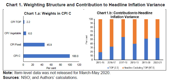 In India, food price inflation followed a downward trajectory till 2018-19 on the back of bumper foodgrains and horticultural production. However, it has started picking up in the following years primarily owing to a rise in vegetable prices. The increase in the incidence of extreme rain events has led to spikes in prices of onions, tomatoes, and potatoes. Vegetables with a weight of 13.2 per cent in CPI-Food and beverages baskets have historically remained one of the major drivers of food inflation (Chart 2). Most of the phases of a pick-up in food prices as well as the subsequent moderations have been led by vegetables. 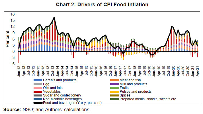 Among vegetables, onions, tomatoes, and potatoes (combined weight of 2.2 per cent in CPI-C and 36.5 per cent in CPI-Vegetables) are the three vegetables consumed commonly in India and are also very vulnerable to supply-side disturbances. These three vegetables have been broadly driving the overall vegetables inflation (Chart 3). The supply disturbances can be natural, such as excess rains, cyclone and drought or man-made namely, strikes, hoarding and speculation. The problem becomes more severe given the relative inelasticity of demand for these key vegetables. Onion price inflation due to its non-substitutability has been the most volatile of the three vegetables in the CPI (Table 1). Another noticeable point is that the volatility in CPI TOP is almost four times the volatility in CPI vegetables excluding TOP underlining the importance of these three vegetables for this study. These three vegetables have contributed significantly to the volatility in vegetable inflation. Consequently, TOP prices have also remained the major driver of volatility in food and beverages inflation. | Table 1: Summary Statistics: CPI Food Inflation (January 2015 to March 2021) | | | Onion | Potato | Tomato | TOP | Vegetables | Veg ex TOP | Food and Beverages | Food Ex TOP | | Mean | 20.0 | 10.2 | 11.6 | 8.0 | 5.3 | 4.0 | 4.4 | 4.2 | | Median | -0.7 | 1.1 | 10.0 | 0.7 | 4.7 | 3.9 | 4.3 | 4.5 | | Maximum | 327.4 | 107.0 | 118.7 | 132.0 | 60.5 | 22.4 | 12.2 | 7.9 | | Minimum | -67.0 | -45.8 | -52.2 | -31.3 | -16.5 | -9.5 | -1.7 | -0.1 | | Std. Dev. | 71.3 | 39.5 | 37.6 | 31.4 | 14.9 | 7.7 | 3.2 | 2.4 | | Skewness | 1.9 | 0.5 | 0.3 | 1.5 | 1.1 | 0.2 | 0.3 | -0.1 | | Kurtosis | 7.5 | 2.4 | 2.8 | 6.1 | 4.9 | 2.5 | 2.5 | 1.6 | | Observations | 71.0 | 71.0 | 71.0 | 71.0 | 75.0 | 71.0 | 75.0 | 71.0 | | Sources: NSO; and Authors’ estimates. | Apart from retail price indices from the CPI data for these vegetables, we also have daily data at retail as well as wholesale level from the Department of Consumer Affairs (DCA), which correlates closely with the CPI data (Chart 4). While CPI data is released at a monthly frequency and comes with a lag, the prices from DCA enable daily tracking of these vegetable prices. All three vegetable prices have their own pattern of seasonality depending on their cropping pattern and arrivals in the market. For instance, tomato prices usually peak during the months of June-July even though its production is reasonably distributed throughout the country and year. Onion production has three seasons - rabi, kharif and late kharif while potato is mainly a rabi crop. The damage to standing or stored crops of these vegetables owing to delayed or extended monsoons, floods, cyclones, and pest attacks can cause demand-supply mismatches leading to a spike in prices. During 2020-21, production deficit in the case of potatoes was caused by unseasonal rains in Uttar Pradesh in March 2020 and cyclone-related damage to the crop in West Bengal in May 2020. This led to a sharp surge in CPI potato inflation from 2.3 per cent in November 2019 to 107.0 per cent in November 2020. Similarly, there was a steep increase in CPI onion inflation to 327.4 per cent in December 2019 due to unseasonal rains during September-October 2019 that damaged the kharif crop in major producing states along with damage to transplantation of the late kharif crop. The data trends reveal that potato prices follow a pattern that is repeated every two years (Chart 4.a). In the case of onion, four peaks can be seen with a gap of around 2.5 years reflecting disturbances from supply-side factors like excess rains (Chart 4.b). Tomato is most perishable and witnesses a greater frequency of such spikes. However, the pickup seen in 2020-21 was quite sharp. Tomato prices usually pick up during summer months (June-July) (Chart 4.c). Further, the impact of any supply shock becomes visible quite quickly. Notably, for all these three vegetables, the correlation between CPI and DCA retail prices is more than 90 per cent. The production of all these three crops has been consistently greater than their estimated demand and yet, there have been spikes in inflation (Chart 5). This points towards supply-side disturbances in these markets. 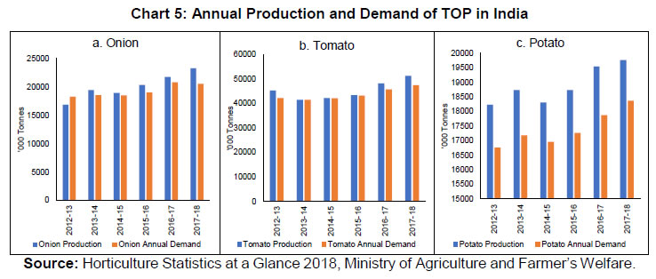 Having analysed the existence of high levels of inflation as well as high volatility associated with these vegetables, the next question is whether there is transmission of volatility from one vegetable to another or across the markets, as the theory of LOP suggests. There could be common driving factors leading to simultaneous spikes, such as increase in input costs, monsoon failures, cyclones and excess rains along with some degree of substitutability and complementarity. Other factors could be hoarding, pest attacks, post-harvest losses and strikes/protests. A cursory look at the DCA price movements indicates that a spike in the price of one vegetable often spreads to another at the retail as well as wholesale level, more so in the case of onion and tomato (Chart 6). Some impact is also seen in the case of potatoes. This kind of co-movement warrants an in-depth analysis of any transmission of volatility from one commodity to another as well as its magnitude. 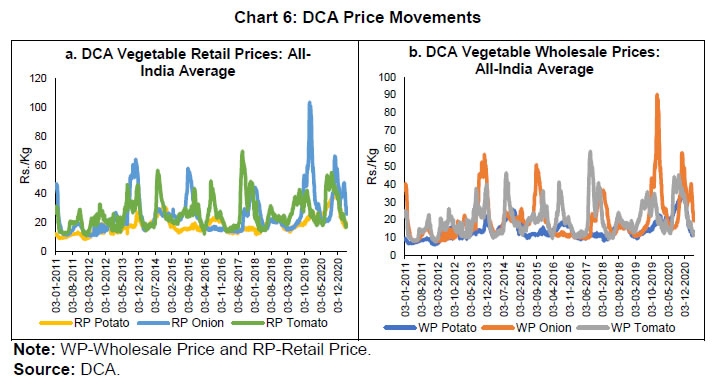 Any spike in prices of the vegetables at the wholesale level gets transmitted to the retail prices or vice versa reflecting vertical integration of the market which depends on costs associated with transportation, retail margins depending on market power, etc. (Chart 7a, 7b, 7c). The direction as well as the speed of transmission warrants a clear understanding so that timely measures can be taken up to contain any inflationary pressures given the sensitivity of headline inflation to vegetable prices as well as the sensitivity of the price of one vegetable to another. 4. Data Description For analysing volatility transmission across the commodities and supply chain, the study uses daily prices data released by the DCA. The sample period of the study spans from January 3, 2011 to March 31, 2021 comprising 3142 data points. The data has been transformed into return series (LnPt - LnPt-1) for estimation purposes. Instead of using CPI data directly, the study uses DCA data mainly due to three reasons. Firstly, the methodology of ARCH/GARCH is more suitable for prices data rather than indices which average out the price levels. Secondly, there are gaps in the item level CPI data during the lockdown period, while DCA data is available even during the period of lockdown, i.e., from March 24, 2020 till May 31, 2020. Finally, DCA data tracks CPI data pretty well in the case of vegetables, giving a strong reason for using DCA data (Chart 4). The Price Monitoring Cell of the DCA collects and monitors daily prices of 22 essential food items from different urban centres spread across the country both at the retail and wholesale level to protect consumers’ interest. Chart 8 reports the commodities currently monitored under DCA. 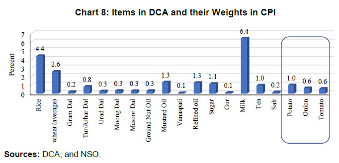 The DCA centres are spread across the North, West, East, South and North-Eastern regions of the country (Appendix Table A1). DCA monitors spot and future prices of selected essential commodities on a daily basis. The prices are reported daily on the website. This study uses spot price data at the all-India level (average of centre-wise data) in the case of vegetables, to analyse the transmission of volatility across the three vegetables (potato, onion, tomato) and across the supply chain, i.e., the transmission mechanism between wholesale and retail prices for each vegetable. The price reporting is not continuous for all the centres. The study uses an average of daily centre-wise prices, which provides an aggregate picture of price movements across vegetables as well as supply chain. The return series of these DCA all-India prices clearly shows the patterns of volatility clustering as large changes are accompanied by large changes and small changes are accompanied by small (Chart 9). Such data characteristics indicate the presence of heteroscedasticity and subsequently ARCH effect in the data. Further, the presence of higher values of kurtosis implies fat tails and that the return series does not follow a normal distribution (Appendix Chart A1). 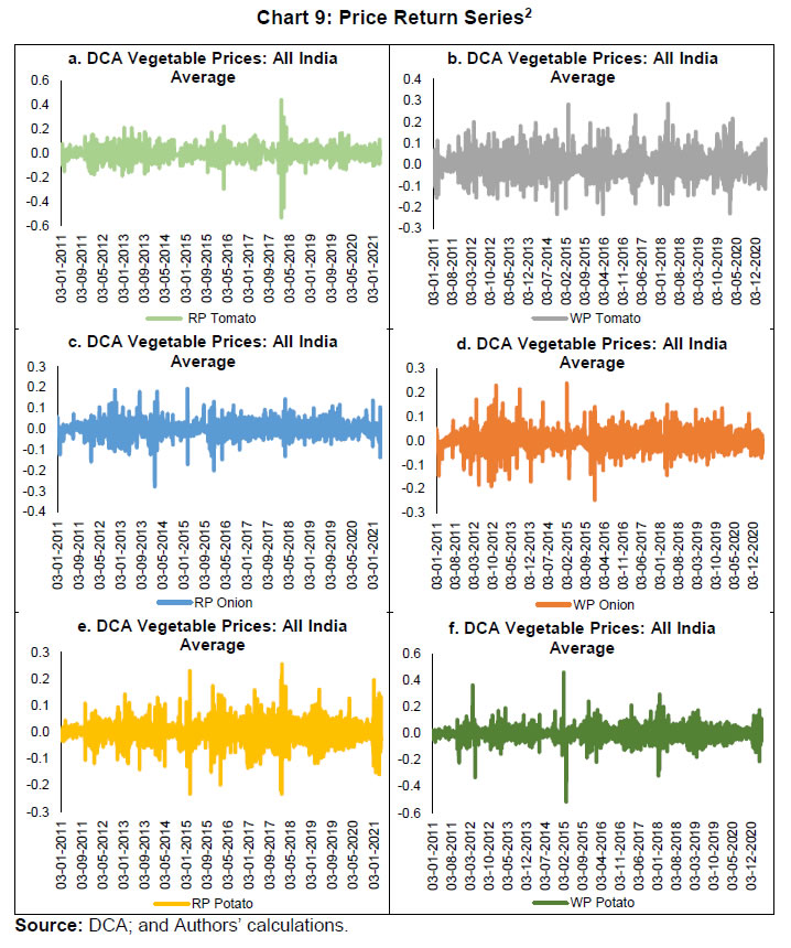 The DCC for each vegetable pair resulting from the Student’s t-DCC (TDCC) model is shown in Chart 10 in terms of retail prices in Panel A and wholesale prices in Panel B. The conditional correlation between retail and wholesale prices reveals a similar pattern of variations. Conditional correlations between vegetables prices (paired) suggest a dynamic relationship. As data for all centres are not reported every day, a few centres have been selected to study the centre-wise volatility patterns. Centres that have reported data for more than 85 per cent of the sample and for which the data gap is not more than 10 days have been considered (Table 2). These data gaps have been filled by taking the average of the last and next observations. | Table 2: Centres Selected | | | Onion | Potato | Tomato | | 1 | Ahmedabad | Ahmedabad | Ahmedabad | | 2 | Bhopal | Bhopal | Bhopal | | 3 | Bhubaneshwar | Bhubaneshwar | Bhubaneshwar | | 4 | Chennai | Chennai | Chennai | | 5 | Delhi | Delhi | Delhi | | 6 | Guwahati | Guwahati | Guwahati | | 7 | Hyderabad | Hyderabad | Hyderabad | | 8 | Jaipur | Jaipur | Kolkata | | 9 | Kolkata | Kolkata | Lucknow | | 10 | Lucknow | Lucknow | Mumbai | | 11 | Mumbai | Mumbai | Shimla | | 12 | Shimla | Shimla | | | Source: DCA. | 5. Methodology 5.1 Volatility Background Volatility is not problematic if prices react to fundamentals like changes in production, stocks and use. Volatility, on the other hand, is harmful when prices fluctuate beyond the underlying fundamentals. Excessive volatility makes resource allocation difficult for stakeholders, namely policymakers, businesses, producers, and consumers. The three most common factors influencing prices are: (1) information flow that varies seasonally depending upon crop productivity; (2) economic factors related to developments on the supply and demand side; and (3) market structure that is influenced by the activities of the speculators, hedgers, and traders in the futures market (Streeter and Tomek, 1992). Regardless of the variations in the underlying theories, the empirical framework and econometric applications for many situations of horizontal price transmission are the same (Listorti and Esposti, 2012). A brief literature review would shed some light on the common methodologies used by researchers for analysing price and volatility transmission. Balcombe and Morrison (2002) and Rapsomanikis et al. (2003) provide a comprehensive analytical framework for the econometric approach to volatility transmission. The findings from these studies suggest that when the cointegration approach and Error Correction Model (ECM) are applied to price series, prices behave differently in the short horizon but converge in the long horizon. Most of the studies have approached market integration from the lens of econometric analysis rather than examining the role of the factors such as transportation systems, interviews with traders, shipment tracking, and exploring unexploited arbitrage opportunities (Baulch, 1997). Volatility and price transmission are linked in the sense that moments of euphoria can cause a momentary rise in volatility (also known as volatility clustering) rather than a temporary or permanent shift in price formation and transmission processes. When analysing the first point, volatility may be viewed as a variation of the residuals of the stochastic process that generated the price series in question. When dealing with the second feature of multivariate GARCH (MGARCH) models (Bollerslev, 1990), we see multivariate stochastic processes, such as those seen in price transmission models, and time-varying variance of one series to transcend to another series. Applying the MGARCH models in price transmission brings out the distinction between market interdependence and contagion more explicitly. Interdependence denotes the regular temporal coupling of processes, whereas contagion denotes the transient increase of this interdependence following a big shock (in tumultuous times) (Bukug et al., 2003). Furthermore, MGARCH models have gained appeal due to their adaptability and ability to provide a concise depiction of the generation and transmission of time-varying volatility across the markets. Abdulai (2007), in his study, emphasised that studies of price transmission largely focus on the nature of the link between prices for different points in the supply chain or marketplaces separated spatially. Spatial transmission is reflected when prices between spatially separated markets tend to be related. The price transmission phenomenon integrates markets vertically and horizontally. Such studies give a great idea about how shocks can be transmitted among one another and act as an indicator of market efficiency. Further research to understand the level of adjustment and speed of shock propagation across producer, wholesale, and retail market prices is critical, as it represents the activities of market actors along the supply chain. 5.2 BEKK Methodology An important observation regarding daily DCA, retail and wholesale price movements is their apparent high level of co-movement which is in line with expectations. Prices of various agricultural commodities fluctuate together on a regular basis (Gilbert, 2010), yet the reasons for the price rises (and volatility) may differ. Several studies have examined the volatility transmission mechanism across two or more financial variables in the past. Most research tools for understanding time-varying variances and covariances are borrowed from a class of models known as Generalised Autoregressive Conditional Heteroscedasticity or GARCH models. GARCH models and their variants are commonly used to measure market price volatility (Kalkuhl et al., 2016). While standard deviation and coefficient of variation are common volatility measurements, their ability to adequately represent price volatility is restricted because they assume price series variance is constant across time. Economists have used numerous thorough and complicated ways to describe price volatility, the most well-known of which are the Autoregressive Conditional Heteroskedasticity (ARCH) model (Engle, 1982) and the Generalised ARCH (GARCH) model (Bollerslev, 1986). ARCH models allow recent shocks to have a favourable impact on present volatility. GARCH models, which expand the ARCH model, presume that earlier shocks and volatilities influence present fluctuations. Equation (1) reports the GARCH (p, q) model as follows: The exponential GARCH (EGARCH) model is an extension of the GARCH model that offers a few benefits over the GARCH model. The most crucial is its logarithmic specification, which permits the positive limitations among the parameters to be relaxed. The EGARCH model also contains asymmetries in return volatilities and effectively captures the permanence of volatility shocks. Equation (2) reports the EGARCH model as follows: The advantage of the GARCH models lies in specifying the equations regarding the movements of the variances and further, MGARCH models are quite successful in predicting the co-movements. Engle and Kroner (1995) developed the Baba-Engle-Kraft-Kroner (BEKK) version of the MGARCH model which has been used in this study to investigate the volatility transmission between the wholesale and retail price changes of vegetables as well as across the vegetables in India. This study employs the full BEKK model from the GARCH family to assess the volatility transmission among the returns of three vegetables (TOP) in one group. Engle and Kroner (1995) developed this model to overcome the limitations of the diagonal VECH models and diagonal BEKK models to enforce positive-definiteness and allow for complicated interactions among the variables. In the diagonal VECH and diagonal BEKK model, the only thing that determines the variance of one series is its past shocks. The BEKK model is the most intuitive technique to handle multivariate matrix operations. In this study, the model is applied to the series residual under the following conditions. The BEKK recursion for Ht is commonly represented as follows: Since our empirical exercise deals with three variables in an equation at a time, we have illustrated a representation of the system BEKK equation with N=3. For such an equation, 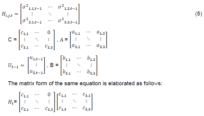
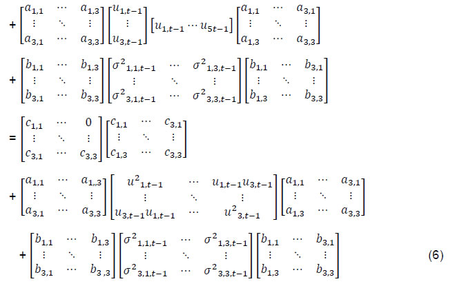 Here C is an N × N lower triangular matrix, and A and B are general N × N matrices that need not be necessarily symmetric. By construction, this is positive semi-definite regardless of the values of the parameters and will maintain positive definiteness, if B or C is a full rank matrix. Considering the above description in equation (6), the BEKK (p,q) model with the aforementioned conditional covariance matrix Ht may be expressed as follows: C is a (3×3) upper triangular matrix of constants with elements of cij, U are the squared lagged errors, A is a (3×3) matrix of aij coefficients that captures the degree of innovation (ARCH Effects), and B is a (3×3) matrix of bij coefficients that represents the volatility persistence and volatility interactions across markets i and j. The BEKK parameterisation of the multivariate GARCH is calculated by maximising the conditional nonlinear log-likelihood function, as described by Engle and Kroner (1995). The Berndt, Hall, and Hausman algorithm was employed for numerical maximisation. The MGARCH models are estimated using the Broyden-Fletcher-Goldfarb-Shanno (BFGS) algorithm using quasi-maximum likelihood estimation (QMLE). In the study, two MGARCH models have been estimated. The estimate of two independent models was done to answer two different questions: one model deals with the volatility dynamics and the temporal evolution of interdependencies (conditional correlations) across tomato, potato, and onion price returns. The BEKK model, in particular, allows for the characterisation of volatility transmission across markets since it is flexible enough to account for own- and cross-volatility spillovers as well as market persistence. Thus, in addition to dealing with the influence of news (both good and negative) in each market on its own volatility, we may also assess how news in one market (for example, potato or tomato) may cause more (lower) volatility in other markets (say onion). Another type of model, DCC and ADCC, generates a Dynamic Conditional Correlation matrix, which allows researchers to examine if the amount of dependency across markets has evolved over time. It solely includes its own symmetric and asymmetric market impacts. 5.3 DCC Methodology Price volatility in a market can be transmitted to other markets. However, the extent and direction may differ subject to the product characteristics, market structure, and country situations impacting volatility dynamics. To understand the dependencies between vegetable price returns, co-movement between the level and second order plays an important role. Correlation (or rolling) analysis is one of the most basic approaches for investigating vegetable market co-movement. A higher degree of correlation between markets suggests better co-movement and market integration. Engle and Sheppard (2001) and Engle (2002) presented the DCC model, a family of multivariate models that is particularly well adapted to studying correlation dynamics among price returns. The fundamental benefit of the DCC model over the BEKK model is that it does not suffer from dimension impediments and may be used in any dimension. This is due to the fact that the estimate may be divided into two steps: first, estimating the univariate GARCH and then creating a maximum likelihood function with just two parameters, the specifics of which are explained in the following paragraphs. The multivariate DCC method combines the flexibility of univariate GARCH with the intricacy of broad multivariate GARCH. Because the parameters to be estimated in the correlation process are independent of the number of series to be correlated, the authors begin the empirical specification by assuming that vegetable returns from the k series are multivariate, normally distributed with zero mean, and have the Ht conditional variance-covariance matrix. The multivariate DCC-GARCH model is illustrated below:
where, D represents a (k×k) diagonal matrix of the conditional volatility of the returns on each asset in the sample, and Rt is the (k×k) conditional correlation matrix. The DCC-GARCH model estimates conditional volatilities and correlations in two steps: Step-1: the mean equation of each asset in the sample, nested in a univariate GARCH model of its conditional variance, is estimated. Hence, Dt can be defined as follows: where, hiit, the conditional variance of each asset, is assumed to follow a univariate GARCH (p, q) process, given by the following equation: However, some constraints as follows, should be enforced to assure non-negativity and stationarity: These univariate variance estimates are then utilised to normalise each asset’s zero mean return innovations. The standardised zero mean return innovations are assumed to follow a multivariate GARCH (m, n) process in the Step-2. To demonstrate the evolution of the time-varying correlation matrix Rt, consider the following: Finally, equation 12 reports the conditional correlation coefficient pij,t between two assets i and j: According to several authors (e.g., Engle and Sheppard, 2001 and Engle, 2002) the T- DCC model can be estimated using a two-stage approach to maximise the log-likelihood function. Let θ denote the parameters in Dt and Φ the parameters in Rt, and then the log-likelihood process can be reported as: 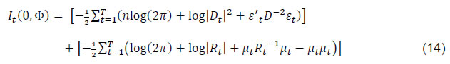 The volatility component of the likelihood function in Equation (14) is the sum of individual GARCH likelihoods. In the first step, the log-likelihood function can be maximised over the parameter in Dt. Considering the estimated parameters from this step, the correlation component of the likelihood function (the second portion of Equation 14) may be maximised in the Step two to estimate the correlation coefficients. In particular, the conditional variance of returns is determined only by previous squared returns, which might lead to the exclusion of volatility transmission. Similarly, the DCC model drastically limits the feedback impact of prior volatilities or squared returns on correlations. This method permits cross-border transmission to fluctuate over time. The Engle and Korner (1995) model is used in this work to capture volatility transmission, while the DCC model is used to assess the dynamic conditional correlation. Employing both BEKK GARCH and multivariate DCC GARCH models in a study provides a greater informational advantage. First, the estimates of BEKK GARCH reveal the magnitude of volatility transmission between the two series. Second, the estimates confirm the direction of volatility transmission, i.e., unidirectional or bi-directional. This also gives us the source of volatility transmission, in terms of net transmitter and net receiver of volatility. Even though the results of BEKK give us the estimates of the transmission of volatility (covariance) and the persistence of volatility, the time-varying strength of the relation between the two series (correlation) is given by the estimates of DCC GARCH. The strength of association between two or more vegetable prices is time varying. The result of multivariate DCC estimates gives us a detailed idea about the same, while the specifics like direction and source are given by estimates of BEKK. Both models, when used simultaneously can offer a comprehensive assessment of the degree of integration of two or more price series. We also study conditional correlation dynamics into a time varying asymmetric framework, applying the technique of AG-DCC model developed by Cappiello et al. (2006) to provide a more robust analysis of spillover. 6. Empirical Analysis The study assesses the interdependence of TOP (Tomato, Onion and Potato) price returns using the approach described in the preceding section. The study employs the complete T-BEKK model and Dynamic Conditional Correlation (T-DCC) specification to explain market interrelationships, volatility transmission, and time changing dependencies across these key vegetable markets utilising daily data frequencies. The long sample period from January 2011 to March 2021 allows us to investigate if the patterns of volatility between vegetable markets have changed in the recent years. The BEKK GARCH approach is used to examine the dependency among TOP prices. This methodology is used to answer two questions. First, whether there is evidence of volatility transmission among TOP price returns, and second, whether there is volatility transmission between retail and wholesale prices for all three vegetables, as well as the direction of volatility transmission. Furthermore, the study used DCC models to study the temporal development of interdependencies (conditional correlations) and volatility dynamics among TOP price returns in both wholesale and retail markets. The methodology used in this study is consistent with a few recent studies, viz., Hernandez et al., 2014 and Gardebroek and Hernandez, 2013. Gardebroek and Hernandez (2013) used typical complete BEKK and DCC models to examine volatility interactions among weekly, ethanol, crude oil and US maize prices and studied if volatility in energy markets increases price volatility in corn markets. In line with our objectives, we present the estimated results in the following manner: first, the centre-wise volatility behaviour for the three vegetables, followed by the cross-vegetable volatility spill over analysis and the transmission of volatility across the supply chain, and finally, we check for time varying correlation structure and asymmetric transmissions, if any. 6.1 Centre-wise Analysis Since the all-India prices are an aggregate of centre-specific prices, we begin by examining volatility behaviour in some of the centres as specified in the preceding section. We examine the centre-wise return of retail prices for each of the three vegetables. In the case of onion and potato, the mean for each centre is close to zero, indicating that there is variability on both sides (Tables 3, 4 and 5). We fitted GARCH models for each centre to describe its volatility since there is evidence of volatility clustering and fat tails in the distribution of all-India return series (which is the average of the centre-wise prices), showing the presence of heteroscedasticity. The total of ARCH and GARCH terms (α and β) in all three vegetables is closer to one for majority of the centres, demonstrating volatility persistence. For onion, the ARCH and GARCH terms are significant in all of the centres. This means that the current volatility of monthly retail price returns may be explained by long-term volatility. As positive and negative shocks may not always have the same influence on prices, we used EGARCH models to describe the centre-wise volatility. | Table 3: Onion Retail Prices Return Series | | | Ahmedabad | Bhopal | Bhubaneswar | Chennai | Delhi | Guwahati | Hyderabad | Jaipur | Kolkata | Lucknow | Mumbai | Shimla | | Mean | 0.000 | 0.000 | 0.000 | 0.000 | 0.000 | 0.000 | 0.000 | 0.000 | 0.000 | 0.000 | 0.000 | 0.000 | | Median | 0.000 | 0.000 | 0.000 | 0.000 | 0.000 | 0.000 | 0.000 | 0.000 | 0.000 | 0.000 | 0.000 | 0.000 | | Maximum | 0.820 | 0.610 | 0.330 | 0.690 | 0.310 | 0.330 | 0.470 | 0.690 | 0.410 | 0.630 | 0.490 | 0.510 | | Minimum | -0.590 | -0.610 | -0.360 | -0.510 | -0.210 | -0.470 | -0.580 | -0.760 | -0.430 | -0.560 | -0.520 | -0.510 | | Std. Dev. | 0.040 | 0.060 | 0.040 | 0.080 | 0.030 | 0.040 | 0.050 | 0.070 | 0.050 | 0.050 | 0.050 | 0.060 | | Skewness | 2.840 | 1.510 | 0.250 | 0.260 | 0.860 | -0.230 | -0.400 | -0.050 | -0.080 | 0.110 | 0.060 | 0.600 | | Kurtosis | 99.540 | 35.550 | 14.720 | 9.550 | 14.120 | 27.920 | 29.190 | 29.580 | 17.260 | 37.400 | 17.170 | 23.360 | | Jarque-Bera | 1224503 | 139904 | 18027 | 5658 | 16588 | 81326 | 89848 | 92492 | 26608 | 154964 | 26306 | 54472 | | Probability | 0.000 | 0.000 | 0.000 | 0.000 | 0.000 | 0.000 | 0.000 | 0.000 | 0.000 | 0.000 | 0.000 | 0.000 | | Sum | -0.130 | -0.300 | -0.740 | -0.820 | -0.730 | -0.360 | -0.640 | -0.980 | -0.510 | -0.460 | -0.710 | -0.760 | | Sum Sq. Dev. | 5.730 | 11.290 | 4.630 | 18.640 | 3.210 | 4.750 | 9.060 | 17.270 | 8.210 | 7.220 | 8.120 | 9.900 | | Observations | 3142 | 3142 | 3142 | 3142 | 3142 | 3142 | 3142 | 3142 | 3142 | 3142 | 3142 | 3142 | | GARCH | | Cst(M) | 0.000 | 0.002 | 0.000 | 0.000 | 0.000 | 0.000 | 0.000 | 0.000 | 0.000 | 0.001 | 0.000 | 0.000 | | P value | 0.000 | 0.000 | 0.000 | 0.000 | 0.000 | 0.000 | 0.000 | 0.000 | 0.000 | 0.000 | 0.000 | 0.000 | | ARCH (α) | 0.017 | 0.044 | 0.038 | 0.042 | 0.075 | 0.021 | 0.019 | 0.050 | 0.029 | 0.097 | 0.127 | 0.039 | | P value | 0.000 | 0.000 | 0.000 | 0.000 | 0.000 | 0.000 | 0.000 | 0.000 | 0.000 | 0.000 | 0.000 | 0.000 | | GARCH (β) | 0.980 | 0.436 | 0.923 | 0.930 | 0.906 | 0.946 | 0.978 | 0.919 | 0.933 | 0.622 | 0.853 | 0.907 | | P value | 0.000 | 0.000 | 0.000 | 0.000 | 0.000 | 0.000 | 0.000 | 0.000 | 0.000 | 0.000 | 0.000 | 0.000 | | EGARCH | | Cst(M) | -0.103 | -2.457 | -0.206 | -0.331 | -0.071 | -6.495 | -0.079 | -0.243 | -0.178 | -1.908 | -0.586 | -0.374 | | P value | 0.000 | 0.000 | 0.000 | 0.000 | 0.000 | -0.010 | 0.000 | 0.000 | 0.000 | 0.000 | 0.000 | 0.000 | | ARCH (α) | 0.074 | 0.119 | 0.071 | 0.102 | 0.031 | 0.010 | 0.063 | 0.116 | 0.064 | 0.255 | 0.230 | 0.121 | | P value | 0.000 | 0.000 | 0.000 | 0.000 | 0.000 | -0.380 | 0.000 | 0.000 | 0.000 | 0.000 | 0.000 | 0.000 | | EGARCH (θ1) | 0.159 | 0.030 | 0.107 | -0.046 | 0.232 | 0.010 | 0.042 | 0.004 | -0.075 | -0.081 | 0.080 | 0.005 | | P value | 0.000 | -0.030 | 0.000 | -0.010 | 0.000 | -0.380 | 0.000 | -0.440 | 0.000 | 0.000 | 0.000 | -0.600 | | EGARCH (θ2) | -0.100 | 0.026 | -0.093 | 0.015 | -0.199 | 0.010 | -0.012 | 0.033 | 0.105 | 0.246 | -0.137 | 0.011 | | P value | 0.000 | -0.030 | 0.000 | -0.040 | 0.000 | -0.190 | 0.000 | 0.000 | 0.000 | 0.000 | 0.000 | -0.260 | | GARCH (β) | 0.987 | 0.570 | 0.973 | 0.947 | 0.992 | 0.010 | 0.990 | 0.962 | 0.974 | 0.702 | 0.927 | 0.943 | | P value | 0.000 | 0.000 | 0.000 | 0.000 | 0.000 | -0.980 | 0.000 | 0.000 | 0.000 | 0.000 | 0.000 | 0.000 | | Source: Authors’ calculations. | For onion, potato, and tomato, the majority of the GARCH factors are significant, showing a dependency on prior volatility, and hence, the persistence in conditional volatility. ARCH coefficients are also substantial, emphasising the effect of previous shocks. The EGARCH coefficient is statistically significant, indicating the presence of asymmetry in majority of the onion, potato, and tomato centres. The asymmetry coefficient (θ1) is positive, indicating that positive residuals increase the variance more than negative residuals, showing that positive price shocks are more disruptive than the negative ones. | Table 4: Potato Retail Prices Return Series | | | Ahmedabad | Bhopal | Bhubaneswar | Chennai | Delhi | Guwahati | Hyderabad | Jaipur | Kolkata | Lucknow | Mumbai | Shimla | | Mean | 0.001 | 0.001 | 0.001 | 0.003 | 0.001 | 0.001 | 0.001 | 0.002 | 0.001 | 0.001 | 0.001 | 0.003 | | Median | 0.000 | 0.000 | 0.000 | 0.000 | 0.000 | 0.000 | 0.000 | 0.000 | 0.000 | 0.000 | 0.000 | 0.000 | | Maximum | 1.060 | 0.667 | 0.670 | 0.670 | 0.410 | 0.880 | 0.780 | 0.670 | 0.440 | 0.880 | 0.380 | 1.000 | | Minimum | -0.640 | -0.500 | -0.500 | -0.440 | -0.200 | -0.390 | -0.480 | -0.380 | -0.430 | -0.560 | -0.390 | -0.550 | | Std. Dev. | 0.040 | 0.050 | 0.050 | 0.070 | 0.030 | 0.040 | 0.050 | 0.050 | 0.040 | 0.050 | 0.040 | 0.070 | | Skewness | 6.170 | 3.730 | 1.760 | 1.190 | 1.460 | 5.390 | 2.800 | 2.670 | 1.200 | 3.310 | 0.380 | 3.790 | | Kurtosis | 170.500 | 59.720 | 41.860 | 14.740 | 25.270 | 110.950 | 61.320 | 39.420 | 39.370 | 77.140 | 15.890 | 52.790 | | Jarque-Bera | 3690799 | 428115 | 199207 | 18784 | 65977 | 1539923 | 449147 | 177249 | 173837 | 724909 | 21830 | 331826 | | Probability | 0.000 | 0.000 | 0.000 | 0.000 | 0.000 | 0.000 | 0.000 | 0.000 | 0.000 | 0.000 | 0.000 | 0.000 | | Sum | 3.310 | 4.320 | 3.830 | 7.890 | 2.030 | 3.230 | 3.560 | 4.850 | 2.860 | 3.930 | 2.640 | 8.280 | | Sum Sq. Dev. | 6.540 | 7.640 | 7.030 | 15.580 | 3.240 | 5.850 | 7.270 | 9.150 | 4.610 | 7.220 | 4.690 | 16.620 | | Observations | 3140 | 3140 | 3140 | 3140 | 3140 | 3140 | 3140 | 3140 | 3140 | 3140 | 3140 | 3140 | | GARCH | | Cst(M) | 0.000 | 0.002 | 0.002 | 0.002 | 0.000 | 0.002 | 0.000 | 0.002 | 0.000 | 0.001 | 0.000 | 0.003 | | P value | -0.260 | 0.001 | -0.006 | -0.026 | -0.070 | -0.010 | -0.320 | -0.010 | -0.200 | -0.060 | -0.250 | 0.000 | | ARCH (α) | 0.093 | 0.047 | 0.076 | 0.015 | 0.050 | 0.033 | 0.044 | 0.103 | 0.036 | 0.049 | 0.073 | 0.107 | | P value | -0.020 | -0.290 | -0.020 | 0.000 | 0.000 | -0.180 | 0.000 | 0.000 | 0.000 | -0.190 | -0.030 | 0.000 | | GARCH (β) | 0.813 | 0.850 | 0.811 | 0.979 | 0.923 | 0.892 | 0.949 | 0.764 | 0.952 | 0.554 | 0.911 | 0.684 | | P value | 0.000 | 0.000 | 0.000 | 0.000 | 0.000 | 0.000 | 0.000 | 0.000 | 0.000 | -0.040 | 0.000 | 0.000 | | EGARCH | | Cst(M) | -0.173 | 0.002 | 0.002 | 0.006 | -0.456 | 0.008 | 0.005 | 0.005 | 0.001 | 0.001 | 0.002 | 0.005 | | P value | 0.000 | -0.050 | -0.010 | 0.000 | 0.00 | -0.130 | -0.150 | -0.030 | -0.190 | -0.030 | 0.000 | -0.040 | | ARCH (α) | 0.0831 | -0.110 | -0.194 | -0.302 | 0.1632 | -0.548 | -0.271 | -0.486 | 0.054 | -1.850 | -0.478 | 1.035 | | P value | 0.000 | -0.820 | -0.660 | -0.315 | 0.00 | -0.158 | -0.235 | 0.000 | -0.940 | -0.430 | 0.000 | -0.570 | | EGARCH (θ1) | 0.161 | 0.030 | 0.053 | -0.068 | -0.079 | -0.273 | -0.106 | -0.154 | 0.036 | -0.116 | -0.014 | -0.115 | | P value | 0.000 | -0.710 | -0.320 | -0.120 | 0.00 | -0.380 | -0.080 | -0.050 | -0.610 | -0.410 | -0.740 | -0.350 | | EGARCH (θ2) | -0.210 | 0.168 | 0.165 | 0.141 | 0.0836 | 0.233 | 0.181 | 0.265 | 0.166 | -0.008 | 0.272 | 0.059 | | P value | 0.000 | -0.160 | 0.000 | 0.000 | 0.00 | -0.440 | 0.000 | 0.000 | 0.000 | -0.930 | 0.000 | -0.370 | | GARCH (β) | 0.976 | 0.671 | 0.825 | 0.948 | 0.943 | 0.955 | 0.976 | 0.871 | 0.658 | 0.485 | 0.944 | 0.867 | | P value | 0.000 | -0.020 | 0.000 | 0.000 | 0.00 | 0.000 | 0.000 | 0.000 | -0.110 | 0.000 | 0.000 | 0.000 | | Source: Authors’ calculations. |
| Table 5: Tomato Retail Prices Return Series | | | Ahmedabad | Bhopal | Bhubaneswar | Chennai | Delhi | Guwahati | Hyderabad | Kolkata | Lucknow | Mumbai | Shimla | | Mean | 0.00 | 0.00 | 0.00 | 0.00 | 0.00 | 0.00 | 0.00 | 0.00 | 0.00 | 0.00 | 0.00 | | Median | 0.00 | 0.00 | 0.00 | 0.00 | 0.00 | 0.00 | 0.00 | 0.00 | 0.00 | 0.00 | 0.00 | | Maximum | 1.25 | 1.07 | 1.14 | 1.16 | 0.93 | 0.72 | 0.92 | 0.85 | 0.85 | 0.57 | 0.69 | | Minimum | -1.02 | -0.62 | -0.69 | -0.92 | -0.36 | -0.47 | -0.69 | -0.63 | -0.63 | -0.29 | -0.79 | | Std. Dev. | 0.06 | 0.08 | 0.12 | 0.12 | 0.05 | 0.05 | 0.08 | 0.08 | 0.08 | 0.06 | 0.11 | | Skewness | 3.94 | 2.04 | 0.59 | 0.49 | 2.65 | 1.69 | 0.70 | 0.60 | 0.60 | 0.80 | 0.19 | | Kurtosis | 185.50 | 40.74 | 10.47 | 10.65 | 44.41 | 64.55 | 27.45 | 21.48 | 21.48 | 11.81 | 12.39 | | Jarque-Bera | 4367262 | 188539 | 7492.74 | 7793.34 | 228155.40 | 497351 | 78504.73 | 44897.24 | 44897.24 | 10501.2 | 11555.33 | | Probability | 0.00 | 0.00 | 0.00 | 0.00 | 0.00 | 0.00 | 0.00 | 0.00 | 0.00 | 0.00 | 0.00 | | Sum | -0.44 | -0.43 | -0.57 | -0.59 | -0.36 | 0.69 | -1.20 | 0.86 | 0.86 | 0.51 | -0.36 | | Sum Sq. Dev. | 10.11 | 21.37 | 43.53 | 48.51 | 9.14 | 7.724006 | 19.14 | 19.61 | 19.61 | 12.04 | 37.97 | | Observations | 3142 | 3142 | 3142 | 3142 | 3142 | 3142 | 3142 | 3142 | 3142 | 3142 | 3142 | | GARCH | | Cst(M) | 0.00 | 0.00 | 0.00 | 0.00 | 0.00 | 0.00 | 0.00 | 0.006 | 0.001 | 0.001 | 0.00 | | P value | 0.00 | 0.00 | 0.00 | 0.00 | 0.00 | 0.00 | 0.00 | 0.00 | 0.00 | 0.00 | 0.00 | | ARCH (α) | 0.0451 | 0.0257 | 0.028 | 0.032 | 0.116 | 0.126 | 0.046 | 0.03 | 0.103 | 0.959 | 0.061 | | P value | 0.00 | 0.00 | 0.00 | 0.00 | 0.00 | 0.00 | 0.00 | 0.00 | 0.00 | 0.00 | 0.00 | | GARCH (β) | 0.727 | 0.95 | 0.933 | 0.962 | 0.671 | 0.593 | 0.94 | 0.86 | 0.706 | 0.25 | 0.93 | | P value | 0.00 | 0.00 | 0.00 | 0.00 | 0.00 | 0.00 | 0.00 | 0.00 | 0.00 | 0.00 | 0.00 | | EGARCH | | Cst(M) | -1.171 | -0.125 | -0.451 | -0.166 | -1.476 | -0.432 | 0.007 | -0.24 | -0.262 | -0.302 | -0.335 | | P value | 0.00 | 0.00 | 0.00 | 0.00 | 0.00 | 0.00 | 0.00 | 0.00 | 0.00 | 0.00 | 0.00 | | ARCH (α) | 0.081 | 0.072 | 0.092 | -0.087 | 0.214 | 0.003 | 0 | 0.068 | 0.105 | 0.116 | 0.185 | | P value | 0.00 | 0.00 | 0.00 | 0.00 | 0.00 | 0.00 | 0.00 | 0.00 | 0.00 | 0.00 | 0.00 | | EGARCH (θ1) | 0.0205 | 0.08 | -0.1 | -0.01 | 0.12 | -0.12 | 0.009 | 0.089 | 0.009 | 0.008 | 0.03 | | P value | 0.10 | 0.14 | 0.00 | 0.40 | 0.00 | 0.00 | 0.00 | 0.00 | 0.02 | 0.00 | 0.054 | | EGARCH (θ2) | -0.131 | -0.035 | 0.047 | -0.008 | -0.0731 | 0.049 | 0.008 | -0.048 | 0.0123 | 0.041 | 0.056 | | P value | 0.00 | 0.00 | 0.00 | 0.00 | 0.00 | 0.00 | 0.00 | 0.00 | 0.0159 | 0.00 | 0.0171 | | GARCH (β) | 0.802 | 0.979 | 0.905 | 0.973 | 0.768 | 0.924 | 0.95 | 0.957 | 0.958 | 0.714 | 0.945 | | P value | 0.00 | 0.00 | 0.00 | 0.00 | 0.00 | 0.00 | 0.00 | 0.00 | 0.00 | 0.00 | 0.00 | | Source: Authors’ calculations. | 6.2 Horizontal Price Transmission across the three Vegetable Prices (Tomato, Onion and Potato) 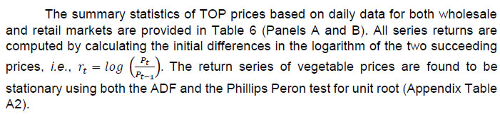 | Table 6A: Summary and Diagnostic Statistics for DCA Vegetable Retail Prices | | DCA Retail Prices | Onion | Potato | Tomato | | Mean | 25.77 | 18.98 | 26.64 | | Median | 21.05 | 17.52 | 23.74 | | Maximum | 103.67 | 46.31 | 69.65 | | Minimum | 10.86 | 8.50 | 11.03 | | No. of Observations | 3167 | 3167 | 3167 | | Price Return Series (D Ln) | | Std. Dev. | 0.03 | 0.04 | 0.05 | | Skewness | 0.01 | 0.12 | -0.29 | | Kurtosis | 10.12 | 9.36 | 17.01 | | Sum | -0.53 | 0.39 | -0.57 | | Sum Sq. Dev. | 2.89 | 3.91 | 6.64 | | Jarque-Bera | 6695.75*** | 5335.448*** | 25933.7*** | | ADF TEST | -7.91*** | -8.05*** | -9.16*** | | Heteroskedasticity Test: ARCH | | F-statistic | 149.7355*** | 355.2837*** | 622.6090*** | | Obs*R-squared | 143.0559*** | 319.5982*** | 520.5122*** | | Correlogram of Residuals | | AC (Lag=1) | 0.000 | -0.07*** | -0.022 | | AC (Lag=2) | 0.021 | -0.215*** | -0.065*** | | Q stat/ Ljung-Box (5) | 105.69*** | 181.41*** | 58.935*** | | Q stat/ Ljung-Box (10) | 387.72*** | 410.61*** | 221.48*** | | Correlogram of Residuals Squared | | AC (Lag=1) | 0.213*** | 0.318*** | 0.406*** | | AC (Lag=2) | 0.1*** | 0.152*** | 0.037*** | | Q stat/ Ljung-Box (5) | 186.21*** | 395.96*** | 529.39*** | | Q stat/ Ljung-Box (10) | 199.69*** | 486.54*** | 546.77*** | | Source: Authors’ calculations. |
| Table 6B: Summary and Diagnostic Statistics for DCA Vegetable Wholesale Prices | | DCA Wholesale Prices | Onion | Potato | Tomato | | Mean | 20.67 | 14.77 | 20.63 | | Median | 16.18 | 13.45 | 18.00 | | Maximum | 90.50 | 40.04 | 58.55 | | Minimum | 7.86 | 6.05 | 7.65 | | No. of Observations | 3167 | 3167 | 3167 | | Price Return Series (D Ln) | | Std. Dev. | 0.03 | 0.04 | 0.05 | | Skewness | 0.19 | -0.04 | 0.27 | | Kurtosis | 8.98 | 18.56 | 6.45 | | Sum | -0.63 | 0.30 | -0.71 | | Sum Sq. Dev. | 3.71 | 6.27 | 7.00 | | Jarque-Bera | 4743.228*** | 31922.69*** | 1606.394*** | | ADF TEST | -7.93*** | -11.89*** | -9.60*** | | Heteroskedasticity Test: ARCH | | F-statistic | 107.3886*** | 36.15329*** | 151.2641*** | | Obs*R-squared | 103.9269*** | 35.76721*** | 144.4496*** | | Correlogram of Residuals | | AC (Lag=1) | -0.005 | -0.050** | -0.009 | | AC (Lag=2) | -0.018 | -0.181*** | -0.038* | | Q stat/ Ljung-Box (5) | 65.105*** | 126.15*** | 43.795*** | | Q stat/ Ljung-Box (10) | 340.34*** | 283.87*** | 285.39*** | | Correlogram of Residuals Squared | | AC (Lag=1) | 0.181*** | 0.106*** | 0.214*** | | AC (Lag=2) | 0.117*** | 0.035*** | 0.059*** | | Q stat/ Ljung-Box (5) | 152.22*** | 39.675*** | 160.88*** | | Q stat/ Ljung-Box (10) | 164.53*** | 45.873*** | 220.71*** | | Source: Authors’ calculations. | Tables 7A and 7B show the BEKK model's estimation results for TOP retail and wholesale prices, respectively. The variance-covariance matrix formulation allows us to examine the direction, size, and persistence of volatility transmission across prices. In matrix notation, the volatility of onion prices is 1, potato price volatility is 2, and tomato price volatility is 3. Thus, price volatility transmission from onion to potato is (1, 2), price volatility transmission from potato to tomato is (2, 3), and price volatility transmission from onion to tomato is (1, 3). The conditional mean equation coefficients are represented by the symbol Yi in Table 7. Both retail and wholesale vegetable prices are statistically significant. The parametric matrix C represents the statistically relevant constant conditional variance-covariance coefficients for TOP markets. For all three vegetables, the impacts of lagged innovation on own return volatility and cross volatility, are substantial at the one per cent level of significance, showing the ARCH effects. At the same time, the diagonal coefficients represent volatility persistence, i.e., the reliance of volatility in market i on previous swings. It demonstrates the GARCH effects. 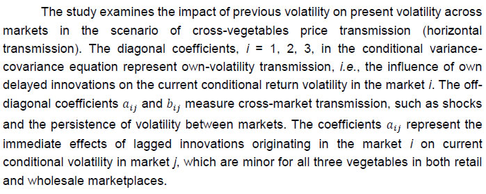
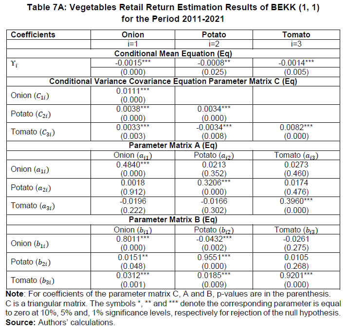
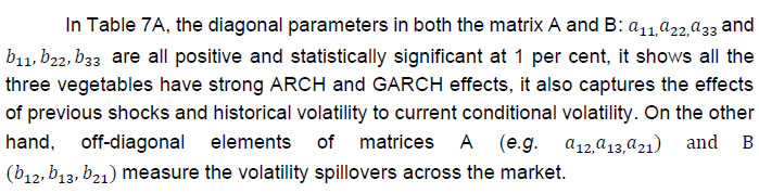 There is no cross transmission of innovations originating in any one vegetable retail prices to other two retail vegetable prices as shown in Table 7A in parameter matrix A. In the case of retail prices, the shock spill over is not statistically significant. Thus, it shows that there is no spill over of return shocks in the case of retail prices except own return shocks. Additionally, when compared to GARCH coefficients, the stated ARCH coefficients are rather small in magnitude. This shows that the conditional volatility of retail prices fluctuates gradually over time rather than changing quickly in response to a shock. It implies that, in contrast to their own shocks, their historical volatility values have a more significant influence in predicting their future volatility. According to the GARCH parameters reported in Table 7A in parameter matrix B, these shocks have a high persistence. These markets may be linked directly by conditional variance and indirectly through conditional covariance. To adequately analyse price interactions, we must account for both direct and indirect impacts. As is typical in these models, the estimated cross effects are often less than the own lag effects. There is bidirectional volatility spillover in the daily retail prices of onion to the potato prices and vice versa. The magnitude of volatility transmission from the onion price to the potato price is (−) 4.32 per cent, whereas the volatility transmission from potato to onion is 1.51 per cent. So, the empirical estimates indicate that the magnitude of volatility spillover from potato prices to onion prices is higher than onion prices to potato prices. The transmission from tomato to potato retail prices and tomato to onion retail prices is unidirectional (Table 7A). A one-per cent increase in the conditional volatility of tomato retail prices appears to result in a 3.12 per cent rise in the volatility of onion retail prices but only a 1.85 per cent increase in potato retail prices. So, the inference from the empirical analysis is that magnitude of tomato retail prices volatility spill over have more impact in the case of onion retail prices compared to potato retail prices as inferred from Table 7A. 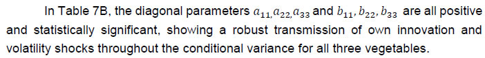 As shown in Table 7B in Parameter matrix A, in the wholesale prices, the impact of shock spill over from tomato to onion prices is unidirectional and negatively significant. This implies that a 1 per cent increase in shock in tomato returns results in a 5.46 per cent decrease in wholesale onion price return volatility (Table 7B). There is no transmission of innovations originating in any of the other two vegetable wholesale prices except tomato wholesale prices to onion wholesale prices. The insignificant spillover effects between the returns of the potato and onion wholesale prices suggests weak integration of the above prices. 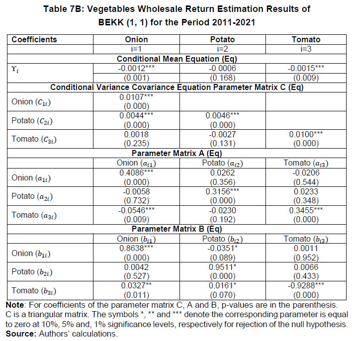 The diagonal coefficients bii in the parameter matrix reported in Table 7B represents the reliance of volatility in prices i on its historical volatility, and the estimates imply that own innovations (information shocks) have a significant direct influence on the associated conditional return volatility in the vegetable prices, as implied by the coefficients' statistical significance. Concerning the dynamics of cross-volatility transmission across the vegetable prices, the off-diagonal coefficients bij represent the direct dependency of volatility in price j on volatility in price i. There is unidirectional volatility spillover in the daily wholesale prices of onion to the potato price. The magnitude of volatility transmission from the onion price to the potato price is (−) 3.51 per cent. The volatility spill over from tomato wholesale price to onion wholesale price is 3.27 per cent. A one-per cent increase in the conditional volatility of tomato wholesale prices appears to result in a 3.27 per cent rise in the volatility of onion wholesale prices. A one-per cent increase in the conditional volatility of tomato wholesale prices appears to result in a 1.61 per cent rise in the volatility of potato wholesale prices. Positive sign of the coefficients indicates that a higher tomato wholesale prices will boost the markets of onion wholesale prices. The findings indicate the prevalence of volatility transmission among TOP prices in India reflecting the role of common driving factors and some degree of substitutability and complimentary among these vegetables. These common factors include common supply shocks- extreme weather shocks (viz. cyclones, monsoon failure, unseasonal rains, droughts, heatwaves etc), hoarding, pest attacks, post-harvest losses and strikes/protests as well as increase in input costs. The TOP prices are essentially interrelated because these vegetables have similar input costs, compete for limited natural resources, and share common market information because of which all the three crops face similar issues with respect to price volatility. The presence of this volatility transmission among TOP prices in India demonstrates the necessity to reduce volatility in the prices of these vegetables and undertake targeted policy intervention. 6.3 Vertical Transmission (Wholesale and Retail Prices) in case of Tomato, Onion and Tomato Tables 8A, 8B and 8C represent the bivariate GARCH estimates for market linkages across the supply chain (wholesale and retail prices) to assess vertical transmission of volatility in the case of onion, potato and tomato prices, respectively. The connection between the retail and wholesale prices can be explained in terms of the magnitude and persistence of shock originating in one market and transmitting to the other market known as vertical price transmission. The diagonal coefficients capture own volatility transmission for each vegetable prices, while the off-diagonal coefficients capture the effect of lagged innovation in the retail prices on the wholesale prices, which is found to be significant in the case of all three vegetables prices. In the case of onion prices, while the transmission of volatility from wholesale to the retail prices is significant, lagged innovation in wholesale prices does not transcend to the retail prices. The potato prices show the transmission of volatility from retail to wholesale prices and vice versa. Potato is relatively more storable compared to tomato and onion. Whenever wholesale price increases, it usually spills over to retail prices. But when retail price spikes because of any issue in the supply chain, the stored potato prices also respond to that shock. It could be because of the storability of potato that we see this bidirectional relation between its retail and wholesale prices. In the case of tomato, the transmission of volatility from wholesale to the retail market is significant, but negative as evident from GARCH coefficients. However, from the significant ARCH coefficients, it is observed that lagged innovations in both retail and wholesale prices for both potato and tomato prices impact each other’s returns in the short run. Interestingly, the strong significance of both ARCH and GARCH coefficients for potato prices show that the returns of retail and wholesale prices are not only affected by their own lagged innovations but also by each other’s lagged volatility fluctuations. As a group, potato retail and wholesale prices show the maximum covariance both in short- and long- run. In fact, the magnitude of covariance, is the highest for potato wholesale prices.
6.4 Time Varying Dynamic Conditional Correlation Analysis (DCC and ADCC) The analysis of dynamic conditional correlation of vegetable returns is another goal of this study. To allow for a time-varying correlation structure, the multivariate DCC model is applied to all three vegetables. The mean equation is represented by parameter ϒ0, whereas the conditional variance of the above-mentioned vegetables is represented by parameters α1, β1 and ω1. All the variables are highly significant and positive. The importance of mean equation parameter ϒ0 demonstrates the dependency of current returns on delayed returns. The conditional heteroskedasticity in the time series is shown by the variance equation parameters α1, β1 and ω1 from the multivariate DCC analysis. The GARCH (1, 1) parameters are extremely significant, supporting the time-varying variance-covariance process and bolstering the DCC model utilised in the analysis. 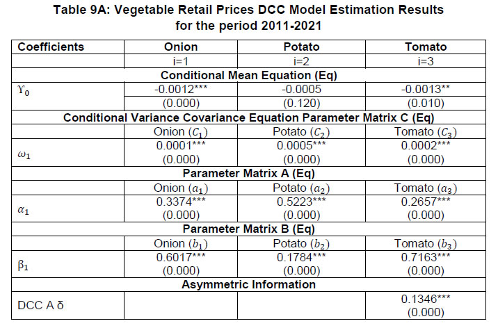 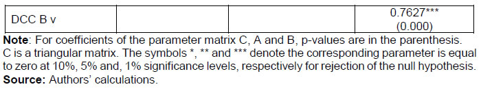
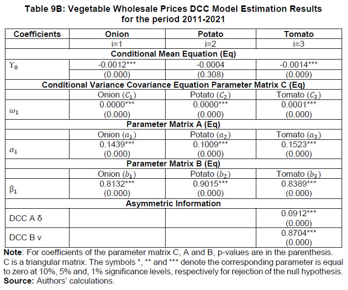 In the case of vegetables retail and wholesale returns, all of the coefficients in a DCC model are important (Table 9A and 9B). The Wald test rejects the null hypothesis that the adjustment parameters are equal to zero at 95 per cent confidence level for the estimated conditional variance and covariances defined in the preceding equations. The coefficient values in Tables 9A and 9B show that volatility persists strongly throughout all series. The computed GARCH coefficients for wholesale price return series are substantial and near to one, showing that wholesale prices are more persistent than retail prices. All (α+β) coefficients are smaller than one, indicating that the unconditional variance is limited. The ARCH parameter DCCAδ in the conditional correlation equation yields modest, positive, and significant estimates, just as the parameters derived from the estimation of the conditional variance process. The GARCH parameters DCCBʋ are big and near to one, suggesting that time-varying correlation is persistent. Finally, the importance of DCC-GARCH estimates (DCCAδ and DCCBʋ) explains why conditional correlations between the three vegetables retail and wholesale prices are dynamic and time-varying. It demonstrates the presence of dynamic conditional connection among the three vegetables prices and is also explored below in detail. 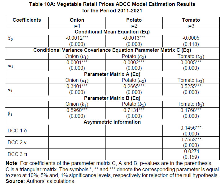
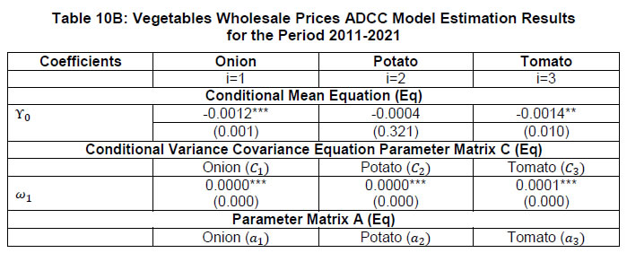 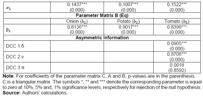 The study also estimates an Asymmetric DCC (ADCC) model, which allows the asymmetric effects of positive and negative shocks. Specifically, a DCC model is calculated under the assumption that the conditional variance follows Nelson's suggested exponential GARCH model (1991). As shown in Tables 10A and 10B, there is no indication of asymmetries in conditional volatility at the conventional level, as the parameter associated with asymmetry or leverage effects DCC 3 π is not statistically significant in the series. So, the study does not find any evidence of a significant differential impact of positive or negative price volatility shocks (asymmetric effects) across these three vegetables in both retail and wholesale markets. 7. Conclusions and Policy Implications This study attempts to comprehend the dynamics of vegetable price volatility in India in the context of three key vegetables- tomato, onion and potato. Firstly, it analyses how volatility behaves in some of the key centres for each selected vegetable. Secondly, it investigates the transmission of volatility across these three vegetables known as horizontal volatility transmission. Thirdly, it aims to understand the volatility transmission between wholesale and retail prices of these three vegetables, called vertical volatility transmission. The study is based on daily DCA data covering the period from January 2011 to March 2021. For testing the robustness of results of BEKK GARCH volatility spill over, DCC methodology has been applied in this study. The centre-wise estimation indicates dependency on prior volatility as well as persistence in the volatility of retail prices in most centres. Further, the estimates indicate the effect of previous shocks and presence of asymmetry in transmission of positive and negative shocks in majority of the onion, potato, and tomato centres. The horizontal price transmission of these three vegetables may be analysed using conditional variance and conditional covariance. In both retail and wholesale markets, there is a unidirectional volatility transmission from tomato prices to those of onions and potatoes. This suggests that knowledge about tomato price variations is passed along to the pricing of potatoes and onions. Further, the magnitude of volatility spillover is greater in the case of tomato to onion prices compared to tomato to potato prices reflecting the greater perishability of onions compared to potatoes. Additionally, there is an evidence of bidirectional transmission of volatility in the case of potato and onion retail prices, demonstrating that the prices of both these commodities interact with each other. The wholesale market volatility transmission from potato to onion prices is unidirectional. The prevalence of volatility transmission in our analysis is the result of market integration. The degree of integration between the tomato, onion, and potato markets also determines the volatility transmission across these three markets. The extent and speed of information flow between prices increase with the degree of integration. This essentially is Cournot's (1927) Law of One Price. TOP prices are also interrelated because they are substitutes in demand to some extent, have similar input costs, compete for limited natural resources, and share common market information. Due to this, all the three crops face similar issues with respect to price volatility. These vegetables are also susceptible to common supply shocks. With respect to the vertical transmission, the potato prices exhibit bidirectional volatility spillovers i.e., from wholesale to retail prices and vice versa. The spillovers from retail to wholesale prices of potato could be attributed to the storability of potato as compared to tomato or onion. As a result, volatility in potato retail prices would also transcend to potato wholesale prices. In the case of tomato and onion, transmission is observed to be unidirectional from wholesale to retail prices. Due to seasonal production, weather disturbances and the inelastic nature of demand, onion wholesale prices volatility continue to transmit to retail prices despite high onion production. Even in the case of tomato where production is well-distributed throughout the year and diversified across states, wholesale price fluctuations are passed on to retail prices since tomatoes are highly perishable and have insufficient storage facilities. Lastly, the study demonstrates a time evolution of dependencies across these vegetables. The level of dependencies between retail and wholesale prices of these three vegetables is dynamic and time-varying. Furthermore, there is no evidence of a differential impact of positive and negative volatility shocks across these three vegetables and hence, there is no indication of asymmetric or leverage effects between retail and wholesale prices of these vegetables. While this study is one of the first few studies to understand the volatility transmission in the case of tomato, onion and potato, there are certain limitations to this study which can be addressed in future research. This study does not look at the factors affecting volatility transmission in the TOP prices which can be undertaken as a part of future research. The potential research for the future could also examine volatility transmission in the case of other agricultural commodities like pulses, vegetable oils, etc. The results of the study can be beneficial for policymakers in various ways. The prevalence of volatility transmission among TOP prices in India demonstrates the necessity to reduce volatility in the prices of these vegetables and undertake targeted policy interventions. This would entail the implementation of various supply-side measures like strengthening of the supply chain, integration of the participants of the value chain, development of ample storage facilities and better post-harvest loss management. Adoption of climate-smart agriculture practices would also help in stabilising prices in the case of supply disruptions due to extreme weather shocks. The understanding of the volatility dynamics in TOP prices would also help in managing price stability.
References Abdulai, A. (2007). Spatial and Vertical price transmission in food staples market chains in Eastern and Southern Africa: What is the evidence. In FAO trade and markets division workshop on staple food trade and market policy options for promoting development in Eastern and Southern Africa, Rome (pp. 1-2). Acharya, S. S., Chand, R., Birthal, P. S., Kumar, S., & Negi, D. S. (2012). Market integration and price transmission in India: A case of rice and wheat with special reference to the world food crisis of 2007/08. Rome: Food and Agriculture Organization, 447-456. Ait Sidhoum, A., & Serra, T. (2016). Volatility spillovers in the Spanish food marketing chain: the case of tomato. Agribusiness, 32(1), 45-63. Andrle, M., & Blagrave, P. (2020). Agricultural Market Integration in India. International Monetary Fund. Areef, M., Rajeswari, S., Vani, N., & Naidu, G. M. (2020). Price Behaviour and Forecasting of Onion Prices in Kurnool Market, Andhra Pradesh State. Economic Affairs, 65(1), 43-50. Apergis, N., & Rezitis, A. (2003). Agricultural price volatility spillover effects: the case of Greece. European Review of Agricultural Economics, 30(3), 389-406 Asche, F., Jaffry, S., & Hartmann, J. (2007). Price transmission and market integration: vertical and horizontal price linkages for salmon. Applied Economics, 39(19), 2535-2545. Balcombe, K. G., & Morrison, J. (2002). Commodity price transmission: A critical review of techniques and an application to selected export commodities. A study for the Food and Agricultural Organization (ESCR) of the United Nations, Rome, Italy. Baquedano, F. G., & Liefert, W. M. (2014). Market integration and price transmission in consumer markets of developing countries. Food Policy, 44, 103-114. Baquedano, F. G., Liefert, W., & Shapouri, S. (2011). World market integration for export and food crops in developing countries: a case study for Mali and Nicaragua. Agricultural Economics, 42(5), 619-630. Baulch, B. (1997). Transfer costs, spatial arbitrage, and testing for food market integration. American Journal of Agricultural Economics, 79(2), 477-487. Bergmann, D., O’Connor, D., & Thümmel, A. (2016). An analysis of price and volatility transmission in butter, palm oil and crude oil markets. Agricultural and Food Economics, 4(1), 1-23. Birthal, P., Negi, A., & Joshi, P. K. (2019). Understanding causes of volatility in onion prices in India. Journal of Agribusiness in Developing and Emerging Economies. Bloch, H., Dockery, A. M., Morgan, C. W., & Sapsford, D. (2007). Growth, commodity prices, inflation and the distribution of income. Metroeconomica, 58(1), 3-44. Bollerslev, T. (1986). Generalized autoregressive conditional heteroskedasticity. Journal of econometrics, 31(3), 307-327. ---(1990). Modelling the coherence in short-run nominal exchange rates: a multivariate generalized ARCH model. The review of economics and statistics, 498-505. Brosig, S., Glauben, T., Götz, L., Weitzel, E. B., & Bayaner, A. (2011). The Turkish wheat market: spatial price transmission and the impact of transaction costs. Agribusiness, 27(2), 147-161. Buguk, C., Hudson, D., & Hanson, T. (2003). Price volatility spillover in agricultural markets: an examination of US catfish markets. Journal of Agricultural and Resource Economics, 86-99. Burman, A., Roy, S., Shah, A., & Patnaik, I. (2018). Diagnosing and overcoming sustained food price volatility: Enabling a National Market for Food. Cappiello, L., Engle, R. F., & Sheppard, K. (2006). Asymmetric dynamics in the correlations of global equity and bond returns. Journal of Financial econometrics, 4(4), 537-572. Cinar, G. (2018). Price volatility transmission among cereal markets. The evidences for Turkey. New Medit, 17(3), 93-104. Conforti, P. (2004). Price transmission in selected agricultural markets. FAO Commodity and trade policy research working paper, 7. Cournot, A. (1927). Researches into the mathematical principles of the theory of wealth, trans. Nathaniel T. Bacon, New York: Macmillan. Dawe, D. (2012). Price Stabilization for Staple Foods: Costs and Benefits, Implications for Modeling, and Using Trade Policy as a Safety Net. Global Uncertainty and the Volatility of Agricultural Commodities Prices, 135. Engle III, R. F., & Sheppard, K. (2001). Theoretical and empirical properties of dynamic conditional correlation multivariate GARCH. Engle, R. F. (1982). Autoregressive conditional heteroscedasticity with estimates of the variance of United Kingdom inflation. Econometrica: Journal of the econometric society, 987-1007. Engle, R. (2002). Dynamic conditional correlation: A simple class of multivariate generalized autoregressive conditional heteroskedasticity models. Journal of Business & Economic Statistics, 20(3), 339-350. Engle, R. F., & Kroner, K. F. (1995). Multivariate simultaneous generalized ARCH. Econometric theory, 11(1), 122-150. Fousekis, P., Katrakilidis, C., & Trachanas, E. (2016). Vertical price transmission in the US beef sector: Evidence from the nonlinear ARDL model. Economic Modelling, 52, 499-506. Ganguly, K., & Gulati, A. (2013). The political economy of food price policy: The case study of India (No. 2013/034). WIDER Working Paper. Gardebroek, C., & Hernandez, M. A. (2013). Do energy prices stimulate food price volatility? Examining volatility transmission between US oil, ethanol and corn markets. Energy economics, 40, 119-129. Gardebroek, C., Hernandez, M. A., & Robles, M. (2016). Market interdependence and volatility transmission among major crops. Agricultural Economics, 47(2), 141-155. Gilbert, C. L. (2010). How to understand high food prices. Journal of agricultural economics, 61(2), 398-425. -- (2010a). Speculative influences on commodity futures prices 2006-2008. Geneva, Switzerland: United Nations Conference on Trade and Development. -- (2012) International agreements to manage food price volatility. Global Food Security, 1(2), 134–142. https://doi.org/10.1016/j.gfs.2012.10.001 Gilbert, C. L., & Morgan, C. W. (2010). Food price volatility. Philosophical Transactions of the Royal Society B: Biological Sciences, 365(1554), 3023-3034. (2010a). Has food price volatility risen. In Technological Studies Workshop on Methods to Analyse Price Volatility. Seville (pp. 28-29). Goodwin, B. K., & Holt, M. T. (1999). Price Transmission and Asymmetric adjustment in the US beef sector. American Journal of Agricultural Economics, 81(3), 630-637. Gulati, A., Wardhan, H., & Sharma, P. (2022a). Tomato, Onion and Potato (TOP) value chains. Agricultural Value Chains in India: Ensuring Competitiveness, Inclusiveness, Sustainability, Scalability, and Improved Finance, 33-97. Gulati, A., Ganguly, K., & Wardhan, H. (2022b). Agricultural Value Chains in India: Ensuring Competitiveness, Inclusiveness, Sustainability, Scalability, and Improved Finance (p. 298). Springer Nature. Hassouneh, I., Serra, T., Bojnec, Š., & Gil, J. M. (2017). Modelling price transmission and volatility spillover in the Slovenian wheat market. Applied Economics, 49(41), 4116-4126. Hernandez, M. A., Ibarra, R., & Trupkin, D. R. (2014). How far do shocks move across borders? Examining volatility transmission in major agricultural futures markets. European Review of Agricultural Economics, 41(2), 301-325. Kalkuhl, M., Von Braun, J., & Torero, M. (2016). Food price volatility and its implications for food security and policy (p. 626). Springer Nature. Kim, D. H., & Lin, S. C. (2012). Inflation and inflation volatility revisited. International finance, 15(3), 327-345. Kinnucan, H. W., & Forker, O. D. (1987). Asymmetry in farm‐retail price transmission for major dairy products. American journal of agricultural economics, 69(2), 285-292. Kishore, V., & Shekhar, H. (2022). Extreme Weather Events and Vegetable Inflation in India. And more..., 65. Lahiani, A., Nguyen, D. K., & Vo, T. (2013). Understanding return and volatility spillovers among major agricultural commodities. Journal of Applied Business Research (JABR), 29(6), 1781-1790. Landes, M. (2008). Indian agriculture and policy in transition. Food for Policy-Reforming Agriculture. Cambridge University. Listorti, G., & Esposti, R. (2012). Horizontal price transmission in agricultural markets: Fundamental concepts and open empirical issues. Bio-Based and Applied Economics, 1(1), 81–108. https://doi.org/10.13128/BAE-10769 Mittal, S., Hariharan, V. K., & Subash, S. P. (2018). Price volatility trends and price transmission for major staples in India. Agricultural Economics Research Review, 31(347-2018-3190), 65-74. Mukherjee, A., Bajaj, P., Kumar, R. & Sebastian, J. (2022). Indian Agriculture: Achievements and Challenges. RBI Bulletin, 2022. Narendra, S. (2014). A study of integration of markets for onion and potato in South Gujarat. International Research Journal of Agricultural Economics and Statistics, 5(2), 241-244. Nayyar, D., & Sen, A. (1994). International trade and the agricultural sector in India. Economic and Political Weekly, 1187-1203. Ozturk, O. (2020). Market integration and spatial price transmission in grain markets of Turkey. Applied Economics, 52(18), 1936–1948. https://doi.org/10.1080/00036846.2020.1726862 Pratap, B., Ranjan, A., Kishore, V., & Bhoi, B. B. (2022). Forecasting Food Inflation using News-based Sentiment Indicators. Reserve Bank of India Occasional Papers, 42(2). Quiroz, J. A., & Soto, R. (1995). International Price Signals in Agricultural Markets: Do Governments Care? Raj, J., Kapur, M., Das, P., George, A. T., Wahi, G., & Kumar, P. (2019). Inflation forecasts: Recent experience in India and a cross-country assessment. The Reserve Bank of India Mint Street Memo No, 19. Rakshit, D., Paul, R. K., & Panwar, S. (2021). Asymmetric price volatility of onion in India. Indian Journal of Agricultural Economics, 76(2), 245-260. Rapsomanikis, G. (2011). Price transmission and volatility spillovers in food markets. Safeguarding food security in volatile global markets, 149-168. Rashid, S., Gulati, A., & Cummings Jr, R. W. (2008). From parastatals to private trade: Lessons from Asian agriculture (Vol. 50). Intl Food Policy Res Inst. Rezitis, A. N., & Stavropoulos, K. S. (2011). Price transmission and volatility in the Greek broiler sector: a threshold cointegration analysis. Journal of Agricultural & Food Industrial Organization, 9(1). Saghaian, S., Nemati, M., Walters, C., & Chen, B. (2018). Asymmetric price volatility transmission between US biofuel, corn, and oil markets. Journal of Agricultural and Resource Economics, 43(1), 46. Saha, N., Kar, A., Jha, G. K., Kumar, P., & Venkatesh, P. (2019). A Study of Market Integration of Tomato in Four Major Markets in India. Indian Journal of Extension Education, 55(4), 128-132. Saha, N., Kar, A., Jha, G.K., Kumar, P., Venkatesh, P., & Kumar, R. R. (2021). Integration of prices in major markets of onion and potato in India. Saxena, R., Paul, R. K., & Kumar, R. (2020). Transmission of price shocks and volatility spillovers across major onion markets in India. Agricultural Economics Research Review, 33(347-2020-1414). Sekhar, C. S. C. (2003). Price formation in world wheat markets—implications for policy. Journal of Policy Modeling, 25(1), 85-106. -- (2012). Agricultural market integration in India: An analysis of select commodities. Food Policy, 37(3), 309–322. https://doi.org/10.1016/j.foodpol.2012.03.002 Sekhar, C. S. C., Roy, D., & Bhatt, Y. (2017). Food inflation and food price volatility in India: Trends and determinants (Vol. 1640). Intl Food Policy Res Inst. --(2018). Food inflation and volatility in India: trends and determinants. Indian Economic Review, 53(1–2), 65–91. https://doi.org/10.1007/s41775-018-0017-z Serra, T. (2011). Food scare crises and price volatility: The case of the BSE in Spain. Food policy, 36(2), 179-185. Serra, T., & Gil, J. M. (2013). Price volatility in food markets: Can stock building mitigate price fluctuations? European Review of Agricultural Economics, 40(3), 507–528. https://doi.org/10.1093/erae/jbs041 Setiya, P., & Muthuselvan, E. R. (2018). A Report on the study of Onion Value Chain. College Of Agricultural Banking. Sharma, R. (2002). The transmission of world price signals: concepts, issues and some evidence from Asian cereal markets. Paper submitted to the OECD Global Forum on Agriculture. OECD CCNM/GF/AGR (2002) 10. Sinha, K., Panwar, S., Alam, W., Singh, K. N., Gurung, B., Paul, R. K., & Mukherjee, A. (2018). Price volatility spillover of Indian onion markets: A comparative study. Streeter, D. H., & Tomek, W. G. (1992). Variability in soybean futures prices: An integrated framework. The Journal of Futures Markets (1986-1998), 12(6), 705. Tadesse, G., Algieri, B., Kalkuhl, M., & von Braun, J. (2014). Drivers and triggers of international food price spikes and volatility. Food Policy, 47, 117–128. https://doi.org/10.1016/j.foodpol.2013.08.014 Timmer, C. P. (1989). Food price policy: The rationale for government intervention. Food Policy, 14(1), 17-27. -- (2008). Causes of high food prices (No. 128). ADB Economics Working Paper Series. Vavra, P., & Goodwin, B. K. (2005). Analysis of price transmission along the food chain. Zorya, S., Cramon-Taubadel, S. V., Greb, F., Jamora, N., Mengel, C., & Würriehausen, N. (2014). Price transmission from world to local grain markets in developing countries: Why it matters, how it works, and how it should be enhanced. Zheng, X., Pan, Z., & Zhuang, L. (2020). Price volatility and price transmission in perishable commodity markets: evidence from Chinese lychee markets. Applied Economics Letters, 27(9), 748-752.
Appendix | Table A1: List of Centres3 | | NORTH ZONE | WEST ZONE | EAST ZONE | SOUTH ZONE | NORTH-EAST ZONE | | Chandigarh | Raipur | Patna | Port Blair | Itanagar | | Delhi | Durg | Bhagalpur | Mayabunder | Guwahati | | Hisar | Ambikapur | Purnia | Vijaywada | Imphal | | Karnal | Bilaspur-cg | Darbhanga | Visakhapatnam | Shillong | | Panchkula | Jagdalpur | Gaya | Kurnool | Tura | | Gurgaon | Panaji | Muzzafarpur | Tirupathi | Jowai | | Shimla | Ahmedabad | Saran | Bengaluru | Aizawl | | Mandi | Rajkot | Munger | Dharwad | Dimapur | | Dharamshala | Surat | Saharsa | Mangalore | Gangtok | | Solan | Bhuj | Madhubani | Mysore | Agartala | | Una | Bhopal | Rohtas (Sasaram) | Bengaluru (east range) | | | Bilaspur-hp | Indore | Motihari | Belagavi | | | Srinagar | Gwalior | Samastipur | Kalaburagi | | | Jammu | Jabalpur | Katihar | Tumakuru | | | Poonch | Rewa | Araria | Bellary | | | Amritsar | Sagar | Nawada | Dhavanagere | | | Ludhiana | Jhabua | Khagaria | Shivamogga | | | Bathinda | Hoshangabad | Ranchi | Vijayapur | | | Lucknow | Shahdol | Gumla | T. Puram | | | Kanpur | Ujjain | Sahibganj | Ernakulam | | | Varanasi | Morena | Bokaro | Kozhikode | | | Agra | Mumbai | Lohardaga | Thrissur | | | Jhansi | Nagpur | Simdega | Palakkad | | | Meerut | Pune | Bhubaneshwar | Wayanad | | | Allahabad | Nashik | Cuttack | Puducherry | | | Gorakhpur | Jaipur | Sambalpur | Chennai | | | Saharanpur | Jodhpur | Rourkela | Dindigul | | | Bareilly | Kota | Berhampur | Thiruchirapalli | | | Ayodhya | Udaipur | Jeypore | Coimbatore | | | Moradabad | Bharatpur | Balasore | Tirunelveli | | | Aligarh | Ajmer | Baripada | Cuddalore | | | Mirzapur (Vindhyanchal) | Bikaner | Balangir | Dharmapuri | | | Dehradun | | Kolkata | Vellore | | | Haldwani | | Siliguri | Ramanathapuram | | | Rudrapur | | Purulia | Hyderabad | | | Haridwar | | Kharagpur | Karimnagar | | | | | Rampurhat | Warangal | | | | | Malda | Adilabad | | | | | Raiganj | Suryapet | | | | | | Jadcherla | | | Source: DCA. |

| Table A2: Unit Root Test Results | | Retail Price Levels | | | Level | Diff | Level | Diff | | | Intercept | Trend and Intercept | | | T stats | P value | T stats | P value | T stats | P value | T stats | P value | | ADF Test | | Onion | -7.64 | 0.00 | -8.14 | 0.00 | -4.96 | 0.00 | -8.12 | 0.00 | | Potato | -3.18 | 0.02 | -7.46 | 0.00 | -3.54 | 0.04 | -7.48 | 0.00 | | Tomato | -5.14 | 0.00 | -11.92 | 0.00 | -5.39 | 0.00 | -11.92 | 0.00 | | Phillips-Perron Test | | Onion | -3.58 | 0.01 | -65.74 | 0.00 | -3.93 | 0.01 | -65.73 | 0.00 | | Potato | -2.53 | 0.11 | -77.25 | 0.00 | -2.93 | 0.15 | -77.26 | 0.00 | | Tomato | -4.39 | 0.00 | -70.73 | 0.00 | -4.62 | 0.00 | -70.72 | 0.00 |
| Wholesale Price Levels | | | Level | Diff | Level | Diff | | | Intercept | Trend and Intercept | | | T stats | P value | T stats | P value | T stats | P value | T stats | P value | | ADF Test | | Onion | -4.69 | 0.00 | -8.33 | 0.00 | -4.87 | 0.00 | -8.32 | 0.00 | | Potato | -2.87 | 0.05 | -11.15 | 0.00 | -3.07 | 0.11 | -11.16 | 0.00 | | Tomato | -5.66 | 0.00 | -9.96 | 0.00 | -5.96 | 0.00 | -9.95 | 0.00 | | Phillips-Perron Test | | Onion | -3.57 | 0.01 | -63.81 | 0.00 | -3.86 | 0.01 | -63.79 | 0.00 | | Potato | -2.78 | 0.06 | -73.94 | 0.00 | -3.07 | 0.11 | -73.95 | 0.00 | | Tomato | -4.40 | 0.00 | -70.04 | 0.00 | -4.61 | 0.00 | -70.03 | 0.00 |
| Retail Price Return Series | | | Level | Diff | Level | Diff | | | Intercept | Trend and Intercept | | | T stats | P value | T stats | P value | T stats | P value | T stats | P value | | ADF Test | | Onion | -7.91 | 0.00 | -20.96 | 0.00 | -7.87 | 0.00 | -20.97 | 0.00 | | Potato | -8.05 | 0.00 | -16.76 | 0.00 | -8.09 | 0.00 | -16.76 | 0.00 | | Tomato | -9.16 | 0.00 | -16.36 | 0.00 | -9.17 | 0.00 | -16.37 | 0.00 | | Phillips-Perron Test | | Onion | -72.71 | 0.00 | -419.62 | 0.00 | -72.67 | 0.00 | -419.46 | 0.00 | | Potato | -82.47 | 0.00 | -462.39 | 0.00 | -82.52 | 0.00 | -462.32 | 0.00 | | Tomato | -71.92 | 0.00 | -436.21 | 0.00 | -71.92 | 0.00 | -436.17 | 0.00 |
| Wholesale Price Return Series | | | Level | Diff | Level | Diff | | | Intercept | Trend and Intercept | | | T stats | P value | T stats | P value | T stats | P value | T stats | P value | | ADF Test | | Onion | -7.93 | 0.00 | -21.25 | 0.00 | -7.89 | 0.00 | -21.27 | 0.00 | | Potato | -11.89 | 0.00 | -17.66 | 0.00 | -11.91 | 0.00 | -17.66 | 0.00 | | Tomato | -9.60 | 0.00 | -18.96 | 0.00 | -9.61 | 0.00 | -18.96 | 0.00 | | Phillips-Perron Test | | Onion | -69.96 | 0.00 | -368.26 | 0.00 | -69.92 | 0.00 | -368.16 | 0.00 | | Potato | -79.57 | 0.00 | -335.63 | 0.00 | -79.60 | 0.00 | -335.56 | 0.00 | | Tomato | -69.55 | 0.00 | -166.89 | 0.00 | -69.54 | 0.00 | -166.86 | 0.00 | | Source: Authors’ estimates. |
|