1. Introduction 2.1 The improvement in State finances achieved in 2021-22 was sustained in 2022-23 by containing gross fiscal deficits (GFDs) within the budget estimates (BE) for the second consecutive year. This consolidation was achieved mainly through reduction in revenue deficits, even as capital outlays remained strong. Budget estimates indicate that prudent fiscal management is also envisaged for 2023-24, with near elimination of revenue deficits. 2.2 The rest of this chapter is divided into seven sections. Section 2 highlights key fiscal indicators of States. Sections 3 and 4 focus on their revenue and expenditure patterns, respectively. Section 5 discusses actual fiscal outcomes during 2023-24 so far and the outlook for the rest of the year. Section 6 details financing of the consolidated fiscal deficit of States. Section 7 provides an overview of their debt position, including contingent liabilities. Section 8 sets out some concluding observations. 2. Key Fiscal Indicators 2.3 States’ consolidated gross fiscal deficit to gross domestic product (GFD-GDP) ratio declined from 4.1 per cent in 2020-21 to 2.8 per cent in 2021-22, led by a moderation in revenue expenditure, coupled with an increase in revenue collection (Table II.1). 2.4 As per the provisional accounts (PA) available from the Comptroller and Auditor General of India (CAG), States GFD-GDP ratio at 2.8 per cent in 2022-23 was below the budget estimate of 3.2 per cent and the Centre’s limit of 4 per cent (Chart II.1a and b). While there was a sharp decline in the revenue deficit, the primary deficit remained sizeable. | Table II.1: Major Deficit Indicators - All States and Union Territories with Legislature | | (₹ lakh crore) | | Item | 2017-18 | 2018-19 | 2019-20 | 2020-21 | 2021-22 | 2022-23 (BE) | 2022-23 (RE) | 2022-23 (PA) | 2023-24 (BE) | | 1 | 2 | 3 | 4 | 5 | 6 | 7 | 8 | 9 | 10 | | Gross Fiscal Deficit | 4.10 | 4.63 | 5.25 | 8.05 | 6.55 | 8.83 | 9.24 | 7.53 | 9.48 | | (Per cent of GDP) | (2.4) | (2.4) | (2.6) | (4.1) | (2.8) | (3.2) | (3.4) | (2.8) | (3.1) | | Revenue Deficit | 0.19 | 0.18 | 1.21 | 3.71 | 1.02 | 0.84 | 1.25 | 0.80 | 0.35 | | (Per cent of GDP) | (0.1) | (0.1) | (0.6) | (1.9) | (0.4) | (0.3) | (0.5) | (0.3) | (0.1) | | Primary Deficit | 1.17 | 1.44 | 1.73 | 4.18 | 2.27 | 4.12 | 4.51 | 3.35 | 4.29 | | (Per cent of GDP) | (0.7) | (0.8) | (0.9) | (2.1) | (1.0) | (1.5) | (1.7) | (1.2) | (1.4) | BE: Budget Estimates. RE: Revised Estimates. PA: Provisional Accounts.
Sources: Budget documents of State governments; and Comptroller and Auditor General of India (CAG). |
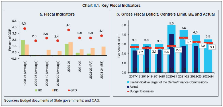 2.5 States have budgeted a GFD-GDP ratio of 3.1 per cent in 2023-24, below the Centre’s limit of 3.5 per cent for the year. At a disaggregated level, 19 States and UTs have budgeted a GFD-GSDP ratio exceeding the FRL1 limit of 3 per cent (Chart II.2; Annex I.1). 3. Receipts 2.6 During 2021-22, States’ revenue receipts increased sharply, following the relaxation of lockdown measures and the rebound in economic activity (Table II.2). The surge in revenue collections was driven by increase in tax revenue - both own taxes and tax devolution - as well as non-tax revenue, offsetting reduced grants from the Centre. 2.7 Within own tax revenue, stamp duty and registration fees, sales tax, and State Goods and Services Tax (SGST) contributed positively to revenue increment (Chart II.3). The strong growth in SGST has been instrumental in reducing the vertical fiscal imbalance between the Centre and the States in recent years (Box II.1). In contrast, States witnessed a fall in revenue from excise duties and taxes and duties related to electricity. Higher non-tax revenue resulted from renewal of existing mining leases and auction of new mines. Within the category of Finance Commission grants, only post-devolution revenue deficit grants witnessed an increase. 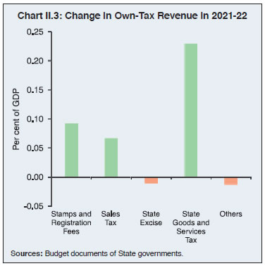
| Table II.2: Aggregate Receipts of State Governments and UTs | | (₹ lakh crore) | | Item | 2018-19 | 2019-20 | 2020-21 | 2021-22 | 2022-23 (RE) | 2022-23 (PA) | 2023-24 (BE) | | 1 | 2 | 3 | 4 | 5 | 6 | 7 | 8 | | 1. Revenue Receipts (a+b) | 26.20 | 26.70 | 25.87 | 32.25 | 39.12 | 36.04 | 43.09 | | | (13.9) | (13.3) | (13.0) | (13.7) | (14.4) | (13.2) | (14.3) | | a. States’ Own Revenue (i+ii) | 14.34 | 14.85 | 13.48 | 17.19 | 20.86 | - | 24.79 | | | (7.6) | (7.4) | (6.8) | (7.3) | (7.7) | - | (8.2) | | i. States’ Own Tax | 12.15 | 12.24 | 11.72 | 14.73 | 18.02 | - | 21.23 | | | (6.4) | (6.1) | (5.9) | (6.3) | (6.6) | - | (7.0) | | ii. States’ Own Non-Tax | 2.19 | 2.61 | 1.76 | 2.47 | 2.84 | 2.78 | 3.56 | | | (1.2) | (1.3) | (0.9) | (1.1) | (1.0) | (1.0) | (1.2) | | b. Central Transfers (i+ii) | 11.87 | 11.85 | 12.39 | 15.06 | 18.26 | - | 18.30 | | | (6.3) | (5.9) | (6.2) | (6.4) | (6.7) | - | (6.1) | | i. Shareable Taxes | 7.47 | 6.51 | 5.95 | 8.83 | 9.48 | - | 10.24 | | | (4.0) | (3.2) | (3.0) | (3.8) | (3.5) | - | (3.4) | | ii. Grants-in Aid | 4.40 | 5.35 | 6.44 | 6.23 | 8.78 | 6.57 | 8.06 | | | (2.3) | (2.7) | (3.2) | (2.7) | (3.2) | (2.4) | (2.7) | | 2. Non-Debt Capital Receipts (i+ii) | 0.42 | 0.57 | 0.23 | 0.22 | 0.14 | 0.09 | 0.43 | | | (0.2) | (0.3) | (0.1) | (0.1) | (0.1) | (0.0) | (0.1) | | i. Recovery of Loans and Advances | 0.41 | 0.57 | 0.13 | 0.20 | 0.11 | 0.09 | 0.20 | | | (0.2) | (0.3) | (0.1) | (0.1) | (0.1) | (0.0) | (0.1) | | ii. Miscellaneous Capital Receipts | 0.01 | 0.00 | 0.10 | 0.02 | 0.03 | 0.00 | 0.24 | | | (0.0) | (0.0) | (0.0) | (0.0) | (0.0) | (0.0) | (0.1) | RE: Revised Estimates. PA: Provisional Accounts. BE: Budget Estimates.
Note: 1. Figures in parentheses are per cent of GDP.
2. -: not available.
Source: Budget documents of State governments; and CAG. |
Box II.1:
Vertical Fiscal Imbalance in India - Changing Dynamics Vertical fiscal imbalance (VFI) - the fiscal gap arising due to the disparity between the revenue generation capacities and expenditure responsibilities across different tiers of government within a federation - impacts government debt and deficits (Aldasoro and Seiferling, 2014; Koley and Mandal, 2019). During periods of increasing imbalances, subnational governments resort to excessive borrowings or neglect the quality of expenditure (Rodden, 2003). It also has a negative effect on gross dometic product (GDP) (Eyruad and Lusiyan, 2013). In India, VFI finds its roots in the asymmetry of revenue-raising authority vested in different tiers of government by the Constitution, with the Centre authorised to levy major taxes while States have higher spending responsibilities (Kelkar, 2019). The Constitution of India empowered the Finance Commissions to suggest transfer of resources from the upper tiers of government to the lower ones to address this imbalance. The implementation of the Goods and Services Tax (GST) could have further impacted VFI, with the States losing control over the value added tax (VAT) which used to be their major source of indirect tax before GST. Following Eyraud and Lusinyan (2013), the VFI is calculated as the share of sub-national own spending2 not financed through own revenues3. 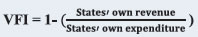 The results indicate that there was no major increase in VFI after the implementation of GST in 2017-18. The VFI moved in a narrow range of 0.48-0.51 during 2017-18 to 2019-20. While there was a spike in VFI in the COVID year (2020-21) due to the widening of gap between the State governments’ own revenue and expenditure, it has declined steadily in the last two years although there are wide variations across States (Charts II.1.1a and II.1.1b). The improvement in the VFI at the aggregate level can be attributed to an increase in own revenue collections by States through SGST which has witnessed a sharp rebound since 2021-22. Thus, contrary to expectations, the introduction of GST has reduced the VFI between the Centre and the States thereby upholding the spirit of fiscal federalism in India. References Aldasoro, I., and Seiferling, M. M. (2014). “Vertical Fiscal Imbalances and the Accumulation of Government Debt”. International Monetary Fund Working Paper 14/29. Eyraud, L., and Lusinyan, L. (2013). “Vertical fiscal imbalances and fiscal performance in advanced economics”. Journal of Monetary Economics, 60(5), 571-587. Kelkar, V. (2019). “Towards India’s new fiscal federalism”. Journal of Quantitative Economics, 17, 237-248. Koley, M., and Mandal, K. (2019). “Vertical fiscal imbalances and its impact on fiscal performance: A case for Indian states”. Opportunities and Challenges in Development: Essays for Sarmila Banerjee, 243-282. Rodden, J. (2003). “Reviving leviathan: fiscal federalism and the growth of government”. International organization, 57(4), 695-729. | 2.8 Provisional accounts indicate that States’ revenue receipts (as a per cent of GDP) fell in 2022-23 due to lower tax revenues and grants from the Centre (Table II.2). For 2023-24, States have budgeted a sharp rise in revenue receipts over 2022-23 (PA), anticipating a broad-based recovery in all major components (Table II.2). SGST, sales tax and States’ excise duties constitute around 79 per cent of the States’ own tax revenue collection (Chart II.4a). The States have budgeted for an acceleration in the growth of sales tax and State excise duty collections. In contrast, the growth in SGST is projected to moderate from a high base (Chart II.4b). Non-tax revenue is budgeted to rise on account of higher collections from renewal of existing mining leases and auction of mines, reforms in power sector, as well as from interest earnings and general services. States need to improve forecast accuracy of revenue estimates, including tax buoyancy, for better fiscal management (Box II.2). 2.9 Several State governments are implementing measures to augment their revenues. For instance, Kerala and Karnataka are aiming to reduce disparities between property guidance values and market values to increase tax collection from registration and stamp duties. Himachal Pradesh’s Sadbhavna Yojana addresses pending cases under different tax Acts. Maharashtra and Rajasthan are contemplating continuation of amnesty programs to resolve pending cases, which in turn is expected to unlock tax arrears receivables. States are also introducing cesses to generate additional revenue. The examples are Kerala’s Social Security cess on Indian Made Foreign Liquor (IMFL) and fuel sales, Goa’s Green cess on non-Goan vehicles, and Himachal Pradesh’s water and milk cess. Delhi will also set up a dedicated Tax Policy and Revenue Augmentation Unit which will use advanced technologies, including data analytics, to boost tax collections. In order to augment non-tax revenues, Kerala is revising mineral royalties. 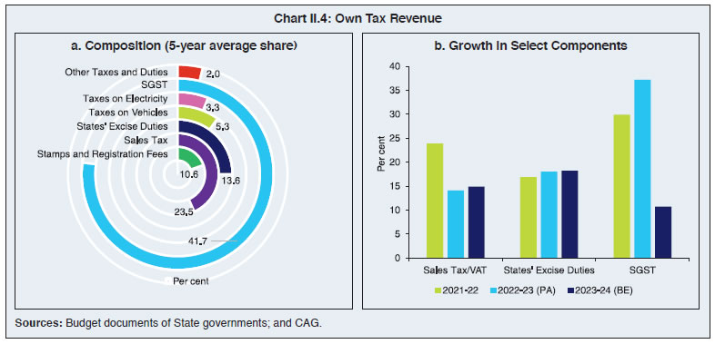
Box II.2:
States’ Own Tax Revenue Buoyancy - Forecasts versus Realisation Robust forecasting of tax buoyancy, a measure of responsiveness of tax revenue to changes in economic activity, is essential for effective budget execution and resource allocation. Large disparities between predicted and actual tax buoyancy can result in inefficient macroeconomic outcomes. For instance, a lower realised revenue relative to estimates would require unforeseen deficit financing, while excess of revenue over the estimates can result in underutilisation of resources and output losses. To examine the forecasting performance of States’ own tax revenue buoyancy, the budgeted and realised buoyancies are calculated with data from 2016-17 to 2022-23 for 13 major States4. The average budgeted buoyancy for the entire sample is 0.74, while the realised buoyancy is lower at 0.55. As the sample period includes two large exogeneous shocks – COVID-19 and Russia-Ukraine conflict - the analysis is also undertaken for two sub-periods –2016-17 to 2019-20 and the period of elevated uncertainty (2020-21 to 2022-23). During the first period (2016-20), the budgeted tax buoyancy was 0.89 (close to unity), while during the period of uncertainty it declined sharply to 0.52. In both cases, however, the realized buoyancy was lower vis-à-vis the forecasts (Chart II.2.1). Forecast errors (actual buoyancy minus budgeted buoyancy) rose during periods of uncertainty (Table II.2.1). In view of this evidence, States would benefit from putting in place appropriate mechanisms to strengthen their forecasting capacity for own revenues for an efficient and optimal use of their budgetary resources. 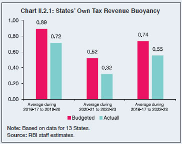
| Table II.2.1: Forecast Errors | | Sample Period | Mean Error | Mean Absolute Error | Root Mean Square Error | U Theil Statistic | | Full Sample | -0.18 | 1.09 | 1.35 | 0.56 | | 2016-17 to 2019-20 | -0.18 | 0.94 | 1.14 | 0.46 | | 2020-21 to 2022-23 | -0.19 | 1.33 | 1.48 | 0.67 | | Source: RBI staff estimates. | | 4. Expenditure Revenue Expenditure 2.10 States’ revenue expenditure (as a per cent of GDP) declined in 2021-22 from the pandemic peak of 2020-21, reflecting fiscal consolidation efforts and reduced needs for COVID-19 related spending (Table II.3). 2.11 Under development expenditure, the allocations for education, sports, art and culture, relief on account of natural calamities, urban development, agriculture and allied activities, and rural development were reduced (Chart II.5a). On the other hand, spending on the power sector and medical and public health increased, the latter reflecting States’ response to the second wave of COVID-19. The decline in non-developmental expenditure was largely broad-based (Chart II.5b). | Table II.3: Expenditure Pattern of State Governments and UTs | | (₹ lakh crore) | | Item | 2018-19 | 2019-20 | 2020-21 | 2021-22 | 2022-23 (RE) | 2022-23 (PA) | 2023-24 (BE) | | 1 | 2 | 3 | 4 | 5 | 6 | 7 | 8 | | Aggregate Expenditure (1+2 or 3+4+5) | 31.25 | 32.52 | 34.15 | 39.02 | 48.50 | 43.66 | 53.01 | | | (16.5) | (16.2) | (17.2) | (16.6) | (17.8) | (16.0) | (17.6) | | 1. Revenue Expenditure | 26.38 | 27.92 | 29.58 | 33.27 | 40.38 | 36.84 | 43.44 | | of which: | (14.0) | (13.9) | (14.9) | (14.2) | (14.8) | (13.5) | (14.4) | | Interest Payments | 3.19 | 3.51 | 3.87 | 4.27 | 4.72 | 4.19 | 5.19 | | | (1.7) | (1.8) | (2.0) | (1.8) | (1.7) | (1.5) | (1.7) | | 2. Capital Expenditure | 4.87 | 4.60 | 4.57 | 5.75 | 8.12 | 6.82 | 9.57 | | of which: | (2.6) | (2.3) | (2.3) | (2.4) | (3.0) | (2.5) | (3.2) | | Capital Outlay | 4.40 | 4.18 | 4.14 | 5.32 | 7.32 | 6.08 | 8.68 | | | (2.3) | (2.1) | (2.1) | (2.3) | (2.7) | (2.2) | (2.9) | | 3. Development Expenditure | 21.01 | 21.63 | 22.64 | 25.99 | 33.22 | - | 36.02 | | | (11.1) | (10.8) | (11.4) | (11.1) | (12.2) | - | (11.9) | | 4. Non-Development Expenditure | 9.44 | 10.05 | 10.64 | 12.04 | 14.13 | - | 15.71 | | | (5.0) | (5.0) | (5.4) | (5.1) | (5.2) | - | (5.2) | | 5. Others* | 0.80 | 0.83 | 0.89 | 0.99 | 1.15 | - | 1.28 | | | (0.4) | (0.4) | (0.4) | (0.4) | (0.4) | - | (0.4) | RE: Revised Estimates. PA: Provisional Accounts. BE: Budget Estimates.
*: Includes grants-in-aid and contributions including compensation and assignments to local bodies.
Notes: 1. Figures in parentheses are per cent of GDP.
2. Capital expenditure includes capital outlay and loans and advances by the State governments.
3. -: not available.
Source: Budget documents of State governments. | 2.12 While revised estimates for 2022-23 suggest higher revenue expenditure by States as per cent of GDP, provisional data5 indicate sharp moderation in spending (Table II.3). In 2023-24, the revenue expenditure of the States is budgeted at 14.4 per cent of GDP with social sector expenditure6 at 8.0 per cent of GDP (Chart II.6a). Committed expenditure, which includes interest payments, administrative services and pensions, declined marginally to 4.5 per cent of GDP in 2022-23 and is expected to remain at the same level in 2023-24 (BE) (Chart II.6b).
Capital Expenditure 2.13 Capital outlay7 of States recorded a robust growth of 28.7 per cent in 2021-22. Strong growth in tax and non-tax revenues and the advancement of payment by the Centre for tax devolution and GST compensation provided the necessary fiscal space to accelerate capital outlay towards agriculture and allied activities, particularly food storage, and warehousing (Chart II.7). Services related to water supply and sanitation, urban development and energy and transport sectors also received higher allocations. As per the provisional accounts, capital outlay of the States increased by 14.3 per cent in 2022-23. Excluding central transfers of ₹0.81 lakh crore under the Scheme for Special Assistance to States for Capital Investment, capital outlay of the States in 2022-23 (PA) at 1.9 per cent of GDP would have been much lower than 2.3 per cent in 2021-22. 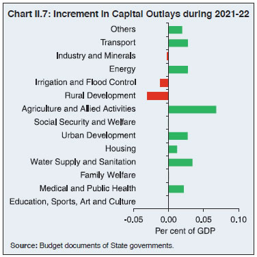 2.14 After a subdued outturn in 2022-23, the capital outlay of the States is budgeted to increase sharply by 42.6 per cent in 2023-24 to 2.9 per cent of GDP. To incentivise States to undertake higher capital expenditure in 2023-24, the Centre has extended the Scheme for Special Assistance to States for Capital Investment with an enhanced loan allocation of ₹1.3 lakh crore (an increase of 30 per cent over a year ago). Expenditure on Research and Development 2.15 Available data for 10 States and UTs8 suggest that their consolidated expenditure on research and development (R&D) rose marginally from 0.07 per cent of their combined GSDP in 2020-21 to 0.10 per cent in 2022-23 (RE), albeit with wide spatial variations (Annex I.2). These States have budgeted R&D expenditure at 0.09 per cent of GSDP for 2023-24. These expenditures are primarily dominated by medical, health, family welfare, sanitation and agricultural research. Over time, the proportion of health-related R&D spending has increased, while spending on agricultural research has declined (Chart II.8). 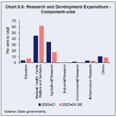 2.16 The overall expenditure quality of the States has improved in the post-pandemic period. The ratio of revenue expenditure to capital outlay (RECO) of the States is budgeted to fall to 5.0 in 2023-24 from 6.0 in 2022-23 (PA). Moreover, the Centre and the States are gradually modernising their banking arrangements, cash management practices and funds transfer mechanisms through adoption of a Single Nodal Agency (SNA) system which would strengthen the public funds disbursal system in India (Box II.3). Box II.3:
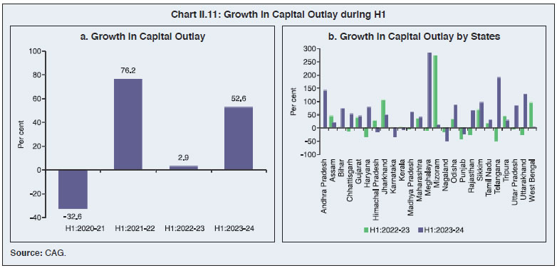
Streamlining Fund Transfers for Efficient Governance - Government’s Cash Management Reforms Efficient banking arrangements and cash management practices are essential for an effective utilisation of government’s financial resources and timely execution of payment obligations. Fragmented banking arrangements - multiple accounts maintained by numerous revenue collecting and spending agencies (including autonomous and statutory bodies) - can result in inefficient cash management practices, with idle cash balance held by some agencies while other agencies facing payment difficulties due to shortage of funds. To fund these cash deficient agencies, the governments resort to short-term borrowings incurring additional interest burden in the process. The Expenditure Management Commission (2015) had recommended that to minimise borrowing costs and to enhance efficiency in fund flows, the government should gradually bring autonomous bodies (ABs) under a consolidated framework of government bank accounts. Such a system, known as Treasury Single Account (TSA), helps to establish comprehensive oversight and centralised control over government’s financial resources and an efficient use of these resources. An effective TSA system is founded on three key principles: (i) unified banking arrangement to promote consolidation of government funds and enable real-time tracking of cash resources; (ii) exclusive treasury oversight, i.e., no government agency other than the Finance Ministry should maintain bank accounts independently; and (iii) comprehensive coverage for complete inclusion of cash balances from all government entities to provide a holistic view of the government’s cash position (IMF, 2011). In India, the TSA system has been adopted in a phased manner, beginning with autonomous bodies and the States and implementing agencies receiving funds under the Central Sector and Centrally Sponsored Schemes (Chart 1). Treasury Single Account (TSA) System for Autonomous Bodies In the first step, various ABs were brought under the TSA system. A TSA for ABs is an assignment bank account opened in the Reserve Bank to receive grants-in-aid from the Centre. More than 200 ABs receive funds through this route (Yadav, 2022). Central Nodal Agency (CNA) System for Central Sector (CS) Schemes The CS schemes are 100 per cent funded by the Union government and implemented by the Central Government machinery. For CS schemes with annual outlays exceeding ₹500 crore, the Centre has made it mandatory that fund transfer should be through the TSA model. Under this, the concerned Ministry designates an agency as the Central Nodal Agency (CNA) for each scheme, with other agencies down the ladder as sub-agencies of the CNA. Each CNA and its sub-agencies open accounts directly with the Reserve Bank, which functions as the primary banker to the Ministry without the involvement of any agency bank. These accounts with the Reserve Bank are assignment accounts wherein an upper limit on expenditure is preassigned. Unutilised assignments lapse to the Centre at the close of the fiscal year and hence are not available to the CNA in the next year. During 2022-23, ₹2.75 lakh crore was allocated to schemes being implemented through the CNA route (Yadav, 2022). In the earlier system, this amount would have moved out of the Centre’s account at the Reserve Bank at the beginning of the fiscal year. For CS Schemes with annual outlays of less than ₹500 crore or schemes being implemented by the agencies of the State governments, the CNAs can open the central nodal account in a commercial bank. Over time, these accounts are expected to migrate to the Reserve Bank as well. 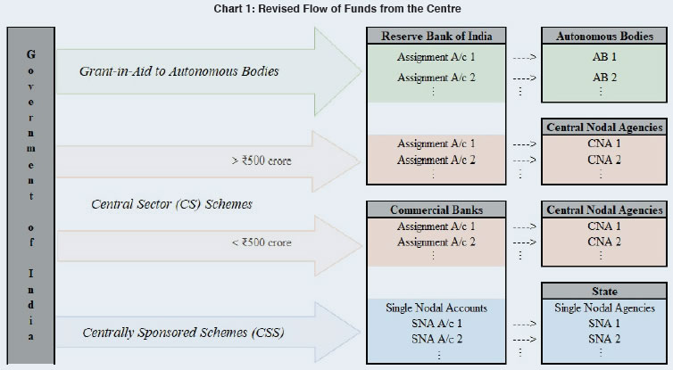 Single Nodal Agency (SNA) Model for Centrally Sponsored Schemes (CSS) The Centre has also notified a new procedure for release of funds under the Centrally Sponsored Schemes (CSS) in which a certain percentage of the funding is borne by the States and the implementation responsibility also lies with the State Governments. Under the new procedure, known as the Single Nodal Agency (SNA) Model, each State designates an SNA to implement a CSS which opens a single nodal account at the State level with a commercial bank. The implementing agencies down the ladder use the SNA’s account through zero balance subsidiary accounts, with predefined drawing limits. The Ministry releases the Centre’s share for each CSS to States’ account with the RBI, which transfers funds to the SNA’s account. Interest earned is remitted to respective governments on a pro-rata basis. Zero balance accounts have eliminated delays, enabling ‘just in time’ payments. More than 3000 SNAs have been onboarded and over eight lakh implementing agencies are now part of this system (GoI, 2023a). For both CS Schemes and CSSs, funds are promptly released from Central Ministries to CNA/SNA and the float in the account is kept at a minimum. The Ministries release only a quarter of the budgeted amount at a time, and the additional funds release is contingent upon utilisation of 75 per cent of the earlier funds. End-year release is avoided to prevent accumulation of unspent balances with the CNAs/ SNAs (GoI, 2023b). Further, the SNA Dashboard launched by the Centre in June 2022 provides comprehensive and real time insights into release, expenditure, account balance and interest earned for each account (GoI, 2022). The dashboard makes the system more transparent while promoting data-driven and better-informed decision-making. This new system of cash management has reduced the number of accounts containing CSS funds from 18 lakh to 3,300 (Yadav, 2022). Estimates suggest that the Centre has saved around ₹10,000 crore through SNA in 2022-23 (Roychoudhury, 2022). The States also benefit from this new system through several ways. First, since expenditure on a CSS in a State is being made from a single account, the submission of utilisation certificates has become easier. Second, by providing data on unspent balances, the government can now see the State-wise float available for a CSS before initiating the proposal for the fund release. Third, the States can also monitor and prioritise the release of new instalments of funds to districts, blocks, and gram panchayats based on their utilisation of the previously allocated funds. Fourth, the States can now monitor the interest credited by the banks and can transfer the States’ share into the consolidated fund of the State. Overall, the ability to see the transaction process end-to-end improves the efficiency of the delivery mechanism. References Department of Expenditure OMs relating to SNA, CNA and TSA: https://doe.gov.in/. GoI (2022). “Union finance minister Smt. Nirmala Sitharaman launches single nodal agency (SNA) dashboard as a part of the azadi ka amrit mahotsav (AKAM) celebrations by ministry of finance in New Delhi.” PIB press release dated June 7, 2022. Available at: https://pib.gov.in/PressReleseDetail.aspx?PRID=1831876. GoI (2023a). “Annual Report 2022-23”, Ministry of Finance. GoI, (2023b). “Compendium of instructions on the new procedure for release of funds under centrally sponsored schemes”, Department of Expenditure, Ministry of Finance. IMF (2011). “Treasury Single Account: An Essential Tool for Government Cash Management”. Prepared by Pattanayak S. and Fainboim I. Fiscal Affairs Department. August. PFMS, Controller General of Accounts (CGA): https://pfms.nic.in/. Roychoudhury, A. (2022). “Govt saved Rs 10,000 crore in interest costs in FY22, says Somanathan”. Business Standard, June 8. Yadav, Sajjan S. (2022). “Financemin’s central nodal agency model: Best value realisation of taxpayers’ money”. The Economic Times, December 3. | 5. Actual Outcome in 2023-24 So Far and Outlook 2.17 During H1:2023-24, States’ consolidated GFD remained higher on a year-on-year (y-o-y) basis, primarily due to lower growth in revenue receipts and robust growth in capital expenditure, even as revenue expenditure growth moderated. Within revenue receipts, growth in tax revenue and non-tax revenue decelerated from a high base. Grants from the Centre contracted sharply with the cessation of GST compensation cess (Chart II.9a). SGST witnessed a robust y-o-y growth of 19.7 per cent, benefitting from the improvement in GST compliance and resilient economic activity (Chart II.9b). Tax devolution from the Centre was buoyant due to high growth in income tax and GST collections and an increase in advance payment of tax devolution of ₹1.18 lakh crore in June 2023 vis-a-vis the normal monthly devolution of ₹0.59 lakh crore. 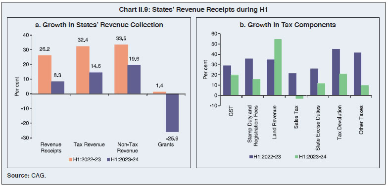 2.18 States’ revenue expenditure growth decelerated to 8.9 per cent in H1:2023-24 (Chart II.10). A similar pattern was observed in revenue expenditure minus interest payments. 2.19 Capital outlay increased by 52.6 per cent during H1:2023-24, driven by support from the Union Government’s Scheme for Special Assistance to States for Capital Investment (Chart II.11 a and b). By end-October, 2023 the Union government had approved expenditure amounting to ₹96,206 crore (accounting for 74.0 per cent of the ₹1.3 lakh crore budgeted for 2023-24) under the scheme, out of which ₹58,494 crore has already been disbursed to the States9. 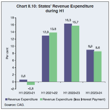
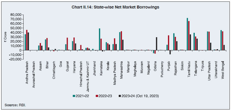
2.20 States’ fiscal outlook remains favourable in view of the resilient domestic economic activity as well as their consolidation efforts. On the revenue side, even though the growth in tax revenue during H1:2023-24 at 14.6 per cent is marginally lower than the budgeted 17.9 per cent, it is expected to improve during H2:2023-24 due to a favourable base and continued robust GST collection. On the expenditure side, growth in the revenue expenditure during the year so far (H1:2023-24) at 8.9 per cent is much lower than the full year budget estimate of 18 per cent and provides space for undertaking higher capex, while persevering with fiscal consolidation. 6. Financing of GFD and Market Borrowings by State Governments and UTs GFD Financing 2.21 On average, net market borrowings financed more than half of the consolidated fiscal deficit of States till 2016-17. Since then, States’ dependence on market borrowings has increased significantly following the recommendation of the Fourteenth Finance Commission (FC-XIV) to exclude States from the National Small Savings Fund (NSSF) financing facility (barring Delhi, Madhya Pradesh, Kerala and Arunachal Pradesh). The reliance on net market borrowings rose to more than 90 per cent in 2019-20. Thereafter, the States’ dependency on net market borrowing has declined and that of loans from the Centre has increased. During 2023-24, States have budgeted to finance 76 per cent of GFD through net market borrowing. Market Borrowings 2.22 The gross market borrowings of States/UTs increased by 8.1 per cent to ₹7.58 lakh crore during 2022-23 from ₹7.02 lakh crore a year ago. The amount borrowed by the States in March 2023 was the highest in the last 5 years (Chart II.12). 2.23 Some States and UTs reduced their gross market borrowings in each of the last two years (Chart II.13a). The consolidated actual borrowings of all States in 2022-23 were 24 per cent lower than the indicative calendar (Chart II.13b). In 2023-24 (till October 19, 2023), their gross market borrowings were 26.4 per cent higher than in the corresponding period of last year, partly due to the base effect (the borrowings had contracted by 7.6 per cent during corresponding period of the last year). 2.24 States’ net market borrowings increased by 5.4 per cent to ₹5.19 lakh crore in 2022-23 from ₹4.92 lakh crore in 2021-22. This increase was concentrated in a few States like Andhra Pradesh, Gujarat, Himachal Pradesh, Madhya Pradesh Haryana and Assam (Chart II.14). 2.25 There were 605 issuances in 2022-23, of which 45 were re-issuances (7.4 per cent) as compared with 608 issuances in 2021-22 and 60 re-issuances (9.9 per cent). Madhya Pradesh, Maharashtra, Puducherry, Punjab, Rajasthan, and Tamil Nadu undertook re-issuances during the year, in line with the policy of passive consolidation10. Out of 350 issuances undertaken by States till October 19, 2023, 30 were re-issuances (Table II.4). 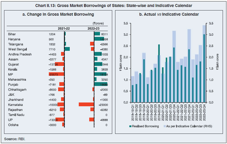
| Table II.4: Market Borrowings of State Governments | | (₹ crore) | | Item | 2019-20 | 2020-21 | 2021-22 | 2022-23 | 2023-24* | | 1 | 2 | 3 | 4 | 5 | 6 | | 1. Maturities during the year | 1,47,067 | 1,47,039 | 2,09,143 | 2,39,562 | 2,89,918# | | 2. Gross sanction under Article 293(3) | 7,12,744 | 9,69,525 | 8,95,166 | 880779 | 7,04,101 | | 3. Gross amount raised during the year | 6,34,521 | 7,98,816 | 7,01,626 | 758392 | 4,06,506 | | 4. Net amount raised during the year | 4,87,454 | 6,51,777 | 4,92,483 | 518830 | 2,68,070 | | 5. Amount raised during the year to total Sanctions (per cent) | 89 | 82 | 78 | 86 | 58 | | 6. Weighted average yield of SGSs (per cent) | 7.24 | 6.55 | 6.98 | 7.71 | 7.44 | | 7. Weighted average spread over corresponding G-Sec (bps) | 55 | 53 | 41 | 31 | 24 | | 8. Average inter- state spread (bps)$ | 6 | 10 | 4 | 3 | 2 | *: As on October 19, 2023.
#: Data for maturity pertain to full year.
$: Based on the cut-off of 10 year fresh issuances.
Source: RBI. |
Table II.5: Maturity Profile of Outstanding State Government Securities
(As at end-March 2023) | | (Per cent) | | State/UT | (Per cent of Total Amount Outstanding) | | less than 1Y | 1 to 5Y | 5 to 10Y | 10 to 20Y | Above 20Y | | 1 | 2 | 3 | 4 | 5 | 6 | | Andhra Pradesh | 4.1 | 29.3 | 28.5 | 38.1 | - | | Arunachal Pradesh | 3.8 | 41.7 | 54.4 | - | - | | Assam | 3.0 | 41.1 | 55.9 | - | - | | Bihar | 9.5 | 47.8 | 42.7 | - | - | | Chhattisgarh | 9.6 | 74.1 | 16.3 | - | - | | Goa | 5.5 | 43.2 | 49.1 | 2.2 | - | | Gujarat | 6.6 | 51.5 | 40.4 | 1.6 | - | | Haryana | 8.1 | 39.0 | 32.8 | 20.1 | - | | Himachal Pradesh | 4.6 | 34.8 | 39.5 | 21.2 | - | | Jammu and Kashmir | 4.2 | 36.0 | 34.3 | 25.5 | - | | Jharkhand | 5.8 | 44.4 | 35.0 | 14.8 | - | | Karnataka | 5.3 | 38.5 | 35.4 | 20.8 | - | | Kerala | 7.9 | 40.9 | 24.7 | 17.1 | 9.3 | | Madhya Pradesh | 6.0 | 38.3 | 27.7 | 26.4 | 1.5 | | Maharashtra | 7.2 | 41.1 | 49.1 | 2.6 | - | | Manipur | 3.7 | 33.6 | 55.7 | 7.1 | - | | Meghalaya | 4.0 | 54.5 | 35.4 | 6.1 | - | | Mizoram | 5.0 | 21.1 | 45.7 | 28.2 | - | | Nagaland | 4.7 | 40.1 | 55.2 | - | - | | Odisha | 22.1 | 38.0 | 25.6 | 14.2 | - | | Puducherry | 7.5 | 44.8 | 37.5 | 10.2 | - | | Punjab | 6.0 | 30.9 | 24.9 | 35.2 | 3.0 | | Rajasthan | 7.2 | 46.1 | 33.0 | 9.3 | 4.4 | | Sikkim | 2.4 | 41.6 | 56.0 | - | 0.0 | | Tamil Nādu | 6.9 | 38.5 | 28.6 | 9.7 | 16.4 | | Telangana | 3.6 | 26.5 | 11.5 | 37.5 | 21.0 | | Tripura | 5.5 | 43.6 | 36.0 | 15.0 | - | | Uttar Pradesh | 2.6 | 41.1 | 48.9 | 7.5 | - | | Uttarakhand | 5.6 | 55.0 | 39.4 | - | - | | West Bengal | 4.9 | 30.4 | 27.4 | 36.9 | 0.4 | | All States and UTs | 5.9 | 39.1 | 34.1 | 17.1 | 3.9 | -: Nil.
Source: RBI. | 2.26 The issuance of 10-year maturity securities constituted 27.9 per cent of the total amount of issuances in 2022-23 as compared with 35.1 per cent in the previous year. The rest 72.1 per cent was spread across maturities, ranging between 2 and 35 years. Reflecting debt consolidation efforts, 55.1 per cent of the outstanding State government securities (SGSs) was in the residual maturity bucket of five years and above as at end-March 2023 (Table II.5). Around 79 per cent of SGS are getting matured during next 10 years, implying higher rollover risk for State governments (Chart II.15a). 2.27 SGS yields traded with an upward bias during 2022-23, reflecting, inter alia, the hike in the policy repo rate by the Reserve Bank and the hardening of the US bond yields (Chart II.15b). Overall, the weighted average cut-off yield (WAY) of SGS issuances rose during 2022-23 to 7.71 per cent from 6.98 per cent in the previous year. The weighted average spread (WAS) of SGS issuances over Central government securities of comparable maturity moderated to 31 bps in 2022-23 from 41 bps in the previous year. Financial Accommodation to States 2.28 As recommended by the Advisory Committee on Ways and Means Advances (WMA) to State Governments, 2021 (Chairman: Shri Sudhir Shrivastava), effective from April 1, 2022, the WMA limit for State governments/UTs was fixed at ₹47,010 crore. State governments/UTs can avail overdraft (OD) on 14 consecutive days and can be in OD for a maximum number of 36 days in a quarter. During 2022-23, 17 States/UTs availed Special Drawing Facility (SDF)11, 12 States/UTs resorted to WMA and 11 States/UTs availed OD. Cash Management of State Governments 2.29 In recent years, States have been accumulating sizeable cash surpluses in intermediate treasury bills (ITBs) and auction treasury bills (ATBs). Although positive cash balances indicate low intra-year fiscal pressure, they involve a negative carry of interest rates, warranting improvement in cash management practices. States’ surplus cash balances declined during 2022-23 as against a sustained increase in 2020-21 and 2021-22 (Table II.6). As on October 18, 2023 States’ consolidated investment in ITBs and ATBs fell to ₹2.03 lakh crore from ₹2.72 lakh crore as at end-March 2023. Table II.6: Investment of Surplus Cash Balance of State Governments/UTs
(Outstanding as on March 31) | | (₹ crore) | | Item | 2020 | 2021 | 2022 | 2023 | 2023* | | 1 | 2 | 3 | 4 | 5 | 6 | | 14-Day (ITBs) | 1,54,757 | 2,05,230 | 2,16,272 | 2,12,758 | 1,08,397 | | ATBs | 33,504 | 41,293 | 87,400 | 58,913 | 95,013 | | Total | 1,88,261 | 2,46,523 | 3,03,672 | 2,71,671 | 2,03,410 | *As on October 18, 2023.
Source: RBI. | States’ Reserve Funds 2.30 Given the increasing borrowing requirements of States and mounting contingent liabilities, they maintain the Consolidated Sinking Fund (CSF) and the Guarantee Redemption Fund (GRF) with the Reserve Bank as a buffer for repayment of future liabilities. States can also avail SDF at a discounted rate from the Reserve Bank against incremental funds invested in CSF and GRF. So far, 24 States and one UT, i.e., Puducherry, have set up CSF and 19 States are members of the GRF (Table II.7). Outstanding investments in CSF and GRF stood at ₹1.8 lakh crore and ₹10,839 crore, respectively, at end-March 2023, as against ₹1.5 lakh crore and ₹9,399 crore, respectively, at end-March 2022. Table II.7: Investment in CSF/GRF by States
(As on March 31, 2023) | | (₹ crore) | | State/UT | CSF | GRF | CSF as per cent of Outstanding Liabilities | | 1 | 2 | 3 | 4 | | Andhra Pradesh | 10,143 | 996 | 2.4 | | Arunachal Pradesh | 2,260 | 4 | 12.0 | | Assam | 5,150 | 78 | 4.1 | | Bihar | 8,164 | - | 2.8 | | Chhattisgarh | 6,447 | - | 5.9 | | Goa | 833 | 401 | 2.7 | | Gujarat | 9,790 | 585 | 2.3 | | Haryana | 1,787 | 1,486 | 0.6 | | Himachal Pradesh | - | - | - | | Jammu & Kashmir UT | - | - | - | | Jharkhand | 1,053 | - | 0.9 | | Karnataka | 14,217 | 313 | 2.7 | | Kerala | 2,613 | - | 0.7 | | Madhya Pradesh | - | 1,119 | - | | Maharashtra | 58,404 | 1,230 | 8.9 | | Manipur | 61 | 123 | 0.4 | | Meghalaya | 1,032 | 82 | 5.5 | | Mizoram | 372 | 66 | 2.9 | | Nagaland | 1,562 | 41 | 9.1 | | Odisha | 15,914 | 1,789 | 12.3 | | Puducherry | 473 | - | 3.8 | | Punjab | 6,437 | 0 | 2.0 | | Rajasthan | - | - | - | | Tamil Nadu | 8,173 | - | 1.1 | | Telangana | 6,915 | 1,512 | 2.0 | | Tripura | 982 | 21 | 4.2 | | Uttar Pradesh | 5,756 | - | 0.8 | | Uttarakhand | 4,305 | 177 | 5.4 | | West Bengal | 11,186 | 816 | 1.9 | | Total | 1,84,029 | 10,839 | 2.5 | ‘-’ : Indicates no fund is maintained.
Source: RBI. | 7. Outstanding Liabilities 2.31 The debt-GDP ratio of States peaked at 31 per cent at end-March 2021 and declined to 27.5 per cent by end-March 2023, supported by fiscal consolidation (Table II.8). At a disaggregated level, the debt to GDP ratio could exceed 25 per cent12 as at end-March 2024 (BE) for 25 States/UTs (Statement 20 and Chart II.16). | Table II.8: Outstanding Liabilities of State Governments and UTs | | Year | Amount | Annual Growth | Debt /GDP | | (End-March) | (₹ lakh crore) | (Per cent) | | 1 | 2 | 3 | 4 | | 2014 | 25.10 | 11.8 | 22.3 | | 2015 | 27.43 | 9.3 | 22.0 | | 2016 | 32.59 | 18.8 | 23.7 | | 2017 | 38.59 | 18.4 | 25.1 | | 2018 | 42.92 | 11.2 | 25.1 | | 2019 | 47.87 | 11.5 | 25.3 | | 2020 | 53.51 | 11.8 | 26.6 | | 2021 | 61.55 | 15.0 | 31.0 | | 2022 | 68.76 | 11.7 | 29.3 | | 2023 (RE) | 74.96 | 9.0 | 27.5 | | 2024 (BE) | 83.32 | 11.2 | 27.6 | RE: Revised Estimates. BE: Budget Estimates.
Sources: 1. Budget documents of State governments.
2. Combined finance and revenue accounts of the Union and the State governments in India, Comptroller and Auditor General (CAG) of India.
3. Ministry of Finance, Government of India.
4. Reserve Bank of India.
5. Finance accounts of the Union government, Government of India. | 2.32 The debt service ratio, measured in terms of interest payment to revenue receipts (IP-RR), saw a sharp increase in 2020-21, but it has gradually moderated thereafter, mainly due to robust revenue receipts (Chart II.17). Composition of Outstanding Liabilities 2.33 The share of outstanding market loans in total debt has been on an upward path in the post-COVID period and is estimated to increase to 66 per cent by end-March 2024 (Table II.9). Similarly, loans from the Centre have also moved higher due to back-to-back loans given to States in lieu of GST Compensation and 50-year interest-free loans distributed under the scheme for Special Assistance to the States for Capital investment as stated earlier. On the other hand, the shares of special securities issued to National Small Saving Funds (NSSF)13, loans from banks and financial institutions and public accounts have witnessed a steady decline. 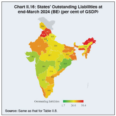
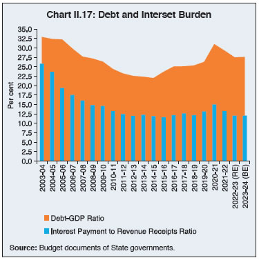
Table II.9: Composition of Outstanding Liabilities of State Governments and UTs
(As at end-March) | | (Per cent) | | Item | 2018 | 2019 | 2020 | 2021 | 2022 | 2023 RE | 2024 BE | | 1 | 2 | 3 | 4 | 5 | 6 | 7 | 8 | | Total Liabilities (1 to 4) | 100.0 | 100.0 | 100.0 | 100.0 | 100.0 | 100.0 | 100.0 | | 1. Internal Debt | 72.7 | 72.2 | 73.5 | 74.0 | 73.0 | 73.4 | 74.5 | | of which: | | | | | | | | | (i) Market Loans | 51.4 | 53.5 | 57.2 | 60.5 | 61.6 | 63.7 | 66.0 | | (ii) Special Securities Issued to NSSF | 11.1 | 9.2 | 7.7 | 6.1 | 5.1 | 4.2 | 3.4 | | (iii) Loans from Banks and Financial Institutions | 4.9 | 4.8 | 4.8 | 4.2 | 3.8 | 3.8 | 3.9 | | 2. Loans and Advances from the Centre | 3.8 | 3.6 | 3.0 | 5.1 | 7.2 | 7.9 | 8.6 | | 3. Public Account (i to iii) | 23.5 | 24.1 | 23.4 | 20.8 | 19.7 | 18.5 | 16.8 | | (i) State PF, etc. | 10.3 | 10.2 | 9.8 | 8.8 | 8.4 | 8.2 | 7.8 | | (ii) Reserve Funds | 4.1 | 4.2 | 3.8 | 3.4 | 3.4 | 3.1 | 2.8 | | (iii) Deposits & Advances | 9.1 | 9.7 | 9.7 | 8.6 | 7.9 | 7.3 | 6.2 | | 4. Contingency Fund | 0.1 | 0.1 | 0.1 | 0.1 | 0.1 | 0.1 | 0.1 | RE: Revised Estimate. BE: Budget Estimate.
Source: Same as that for Table II.8. | Contingent Liabilities of States 2.34 After declining to 2 per cent of GDP by March 2017, State government guarantees gradually rose to 3.8 per cent by end-March 2021. They remained at an elevated level till end March 2022, with adverse implications for debt sustainability (Table II.10). Data available for 18 States and UTs indicate that outstanding guarantees decreased by around 16 per cent during 2022-23. | Table II.10: Guarantees Issued by State Governments | Year
(End-March) | Guarantees Outstanding | | ₹ lakh crore | As per cent of GDP | | 1 | 2 | 3 | | 2014 | 3.79 | 3.4 | | 2015 | 4.28 | 3.4 | | 2016 | 3.64 | 2.6 | | 2017 | 3.12 | 2.0 | | 2018 | 4.30 | 2.5 | | 2019 | 5.38 | 2.8 | | 2020 | 5.93 | 3.0 | | 2021 | 7.60 | 3.8 | | 2022 | 8.90 | 3.8 | | Source: State governments and CAG. | 8. Conclusion 2.35 The debt-GDP ratio of States declined to 27.5 per cent as at end-March 2023 from the peak of 31 per cent at end-March 2021. At the individual level, however, the debt-GDP ratio for some States remains high. The support received from the Centre in the form of 50-year interest free capex loans has helped in reducing States’ interest burden. The overall fiscal outlook for States remains favourable in 2023-24, with adequate fiscal space for undertaking higher capex.
Annex I.1
Deficit Indicators - State-wise | | (Per cent of GSDP) | | State | GFD | RD | PD | | 2021-22 | 2022-23 (RE) | 2023-24 (BE) | 2021-22 | 2022-23 (RE) | 2023-24 (BE) | 2021-22 | 2022-23 (RE) | 2023-24 (BE) | | 1 | 2 | 3 | 4 | 5 | 6 | 7 | 8 | 9 | 10 | | 1 | Andhra Pradesh | 2.2 | 3.6 | 3.8 | 0.8 | 2.2 | 1.5 | 0.3 | 1.7 | 1.8 | | 2 | Arunachal Pradesh | 3.1 | 7.5 | 5.9 | -15.3 | -14.6 | -7.1 | 0.9 | 5.2 | 3.7 | | 3 | Assam | 4.4 | 8.1 | 3.7 | 0.2 | 3.0 | -0.5 | 2.9 | 6.6 | 2.1 | | 4 | Bihar | 3.9 | 9.2 | 3.0 | 0.1 | 3.8 | -0.5 | 1.8 | 7.1 | 0.8 | | 5 | Chhattisgarh | 1.5 | 3.2 | 3.0 | -1.1 | -0.6 | -0.7 | 0.0 | 1.6 | 1.6 | | 6 | Goa | 3.2 | 5.1 | 4.7 | -0.1 | -0.6 | -0.7 | 1.0 | 2.9 | 2.5 | | 7 | Gujarat | 1.2 | 1.5 | 1.8 | -0.3 | -0.3 | -0.4 | -0.1 | 0.3 | 0.6 | | 8 | Haryana | 3.6 | 3.3 | 3.0 | 2.3 | 1.8 | 1.5 | 1.5 | 1.2 | 1.1 | | 9 | Himachal Pradesh | 3.0 | 6.4 | 4.6 | -0.6 | 3.2 | 2.2 | 0.3 | 3.9 | 2.0 | | 10 | Jharkhand | 0.7 | 2.2 | 2.7 | -1.9 | -2.4 | -3.1 | -1.0 | 0.5 | 1.1 | | 11 | Karnataka | 3.3 | 2.7 | 2.5 | 0.7 | 0.3 | 0.5 | 2.1 | 1.4 | 1.2 | | 12 | Kerala | 4.9 | 3.5 | 3.4 | 3.2 | 1.9 | 2.1 | 2.4 | 1.1 | 1.2 | | 13 | Madhya Pradesh | 3.3 | 3.6 | 3.8 | -0.4 | -0.1 | 0.0 | 1.7 | 2.0 | 2.3 | | 14 | Maharashtra | 2.1 | 2.7 | 2.5 | 0.5 | 0.6 | 0.4 | 0.8 | 1.4 | 1.2 | | 15 | Manipur | 4.9 | 6.4 | 5.7 | -4.0 | -15.0 | -14.9 | 3.0 | 4.2 | 3.7 | | 16 | Meghalaya | 5.6 | 4.4 | 3.3 | -1.7 | -3.5 | -4.7 | 3.1 | 1.9 | 0.9 | | 17 | Mizoram | 1.3 | 7.0 | 3.2 | -2.2 | -1.3 | -1.1 | -0.3 | 5.2 | 1.5 | | 18 | Nagaland | 0.8 | 6.3 | 2.7 | -5.1 | -3.3 | -1.7 | -2.1 | 3.2 | -0.1 | | 19 | Odisha | -3.1 | 2.8 | 3.0 | -6.5 | -2.3 | -3.1 | -4.0 | 1.9 | 2.1 | | 20 | Punjab | 4.5 | 4.9 | 4.7 | 3.0 | 3.5 | 3.3 | 1.4 | 1.9 | 1.7 | | 21 | Rajasthan | 4.0 | 4.3 | 4.0 | 2.1 | 2.3 | 1.6 | 1.7 | 2.2 | 1.9 | | 22 | Sikkim | 2.4 | 4.4 | 4.3 | -1.1 | -2.0 | -0.1 | 0.7 | 2.7 | 2.5 | | 23 | Tamil Nadu | 4.0 | 3.2 | 3.4 | 2.2 | 1.3 | 1.4 | 1.9 | 1.2 | 1.4 | | 24 | Telangana | 4.1 | 3.8 | 4.0 | 0.8 | -0.2 | -0.3 | 2.4 | 2.4 | 2.4 | | 25 | Tripura | -0.1 | 4.0 | 5.3 | -2.4 | -0.6 | 0.0 | -2.3 | 2.0 | 3.5 | | 26 | Uttar Pradesh | 2.0 | 3.6 | 3.2 | -1.7 | -2.4 | -2.6 | -0.2 | 1.6 | 1.3 | | 27 | Uttarakhand | 1.4 | 2.7 | 2.7 | -1.5 | -0.8 | -1.3 | -0.4 | 0.7 | 0.9 | | 28 | West Bengal | 3.7 | 4.0 | 3.8 | 2.3 | 2.6 | 1.8 | 1.0 | 1.4 | 1.3 | | 29 | Jammu and Kashmir | 5.6 | 3.1 | 4.7 | 0.0 | -8.6 | -8.3 | 1.9 | -0.9 | 1.0 | | 30 | NCT Delhi | 0.8 | 0.4 | 0.9 | -0.4 | -0.9 | -0.5 | 0.4 | 0.1 | 0.6 | | 31 | Puducherry | -0.1 | 0.0 | 1.8 | -0.5 | -1.0 | 0.2 | -2.1 | -1.9 | -0.2 | | | All States and UTs | 2.8 | 3.4 | 3.1 | 0.4 | 0.5 | 0.1 | 1.0 | 1.7 | 1.4 | RE: Revised Estimates. BE: Budget Estimates. RD: Revenue Deficit. GFD: Gross Fiscal Deficit.
PD: Primary Deficit.
Note: Negative (-) sign in deficit indicators indicates surplus.
Source: Budget documents of State governments. |
Annex I.2
States' Expenditure on Research and Development (R&D) | | (₹ Crore) | | | 2019-20 | 2020-21 | 2021-22 | 2022-23 (RE) | 2023-24 (BE) | | Bihar | | Total R&D (a to g) | 14.9 | 15.3 | 30.5 | 62.8 | 114.3 | | | (0.00) | (0.00) | (0.00) | (0.01) | (0.01) | | a. Education | | | | | | | b. Medical, Health, Family Welfare and Sanitation | | | | | | | c. Agricultural Research | 2.5 | 2.0 | 1.4 | 4.1 | 12.6 | | d. Industrial Research | | | | | | | e. Environmental Research | | | | | | | f. Infrastructure Research | | | | | | | g. Others | 12.4 | 13.3 | 29.1 | 58.8 | 101.8 | | Haryana | | Total R&D (a to g) | 513.5 | 561.8 | 647.2 | 717.2 | 297.6 | | | (0.07) | (0.08) | (0.07) | (0.07) | (0.03) | | a. Education | 18.5 | 13.0 | 14.6 | 25.7 | 18.5 | | b. Medical, Health, Family Welfare and Sanitation | 0.0 | 0.8 | 1.0 | 0.4 | 0.5 | | c. Agricultural Research | 434.7 | 504.9 | 602.4 | 654.3 | 227.5 | | d. Industrial Research | | | | | | | e. Environmental Research | 4.0 | 3.7 | 5.7 | 2.9 | 0.6 | | f. Infrastructure Research | 55.2 | 38.7 | 22.3 | 28.9 | 50.0 | | g. Others | 1.1 | 0.8 | 1.2 | 5.1 | 0.4 | | Jammu and Kashmir | | Total R&D (a to g) | 65.2 | 68.1 | 77.2 | 115.6 | 79.7 | | | (0.04) | (0.04) | (0.04) | (0.05) | (0.03) | | a. Education | 0.0 | 10.8 | 2.0 | 3.8 | 26.9 | | b. Medical, Health, Family Welfare and Sanitation | 2.3 | 3.0 | 3.2 | 6.9 | 5.3 | | c. Agricultural Research | 55.4 | 46.7 | 60.3 | 76.5 | 44.5 | | d. Industrial Research | 0.0 | 0.0 | 0.0 | 0.0 | 0.0 | | e. Environmental Research | 0.0 | 0.0 | 0.0 | 0.0 | 0.0 | | f. Infrastructure Research | 7.6 | 7.5 | 7.3 | 25.3 | 3.0 | | g. Others | 0.0 | 0.1 | 4.6 | 3.1 | 0.0 | | Karnataka | | Total R&D (a to g) | 2061.4 | 1798.7 | 1826.9 | 1903.7 | 2051.6 | | | (0.13) | (0.11) | (0.09) | (0.08) | (0.08) | | a. Education | 48.3 | 40.5 | 41.5 | 50.1 | 51.7 | | b. Medical, Health, Family Welfare and Sanitation | 623.2 | 636.4 | 647.3 | 888.3 | 956.7 | | c. Agricultural Research | 957.7 | 652.4 | 647.3 | 573.6 | 637.4 | | d. Industrial Research | 6.5 | 4.6 | 4.8 | 0.9 | 0.8 | | e. Environmental Research | 36.3 | 62.9 | 59.8 | 22.0 | 18.4 | | f. Infrastructure Research | | | | | | | g. Others | 389.4 | 401.8 | 426.2 | 368.9 | 386.5 | | Odisha | | Total R&D (a to g) | | 388.8 | 550.7 | 937.5 | 1216.3 | | | | (0.07) | (0.08) | (0.12) | (0.14) | | a. Education | | 125.5 | 195.3 | 298.4 | 500.1 | | b. Medical, Health, Family Welfare and Sanitation | | 25.7 | 29.8 | 73.7 | 105.8 | | c. Agricultural Research | | 24.6 | 96.6 | 175.7 | 199.2 | | d. Industrial Research | | 2.2 | 2.0 | 3.0 | 22.7 | | e. Environmental Research | | 15.6 | 12.9 | 20.3 | 17.9 | | f. Infrastructure Research | | 38.8 | 56.9 | 90.1 | 81.1 | | g. Others | | 156.3 | 157.3 | 276.5 | 289.6 | | Rajasthan | | Total R&D (a to g) | 2268.0 | 2356.2 | 2993.1 | 6309.4 | 6143.1 | | | (0.23) | (0.23) | (0.25) | (0.45) | (0.39) | | a. Education | 10.2 | 20.9 | 16.8 | 73.3 | 83.9 | | b. Medical, Health, Family Welfare and Sanitation | 1800.7 | 1977.5 | 2571.8 | 5746.2 | 5438.7 | | c. Agricultural Research | 305.7 | 284.0 | 303.8 | 350.4 | 435.3 | | d. Industrial Research | 0.0 | 0.0 | 0.2 | 0.8 | 0.5 | | e. Environmental Research | 3.6 | 3.2 | 5.0 | 8.3 | 5.5 | | f. Infrastructure Research | 77.8 | 41.7 | 45.4 | 49.7 | 72.4 | | g. Others | 69.9 | 28.9 | 50.1 | 80.7 | 106.8 | | Sikkim | | Total R&D (a to g) | 4.1 | 4.4 | 3.6 | 11.1 | 14.7 | | | (0.01) | (0.01) | (0.01) | (0.03) | (0.03) | | a. Education | 0.1 | 0.3 | 0.3 | 0.7 | 1.0 | | b. Medical, Health, Family Welfare and Sanitation | 0.3 | 0.0 | 0.0 | 0.1 | 0.7 | | c. Agricultural Research | 0.0 | 0.1 | 0.1 | 0.2 | 0.2 | | d. Industrial Research | | | | | 0.6 | | e. Environmental Research | 3.6 | 3.8 | 3.0 | 9.5 | 11.1 | | f. Infrastructure Research | | | | | | | g. Others | 0.1 | 0.2 | 0.2 | 0.6 | 1.2 | | Tamil Nadu | | Total R&D (a to g) | 176.2 | 530.1 | 428.0 | 411.1 | 407.4 | | | (0.01) | (0.03) | (0.02) | (0.02) | (0.02) | | a. Education | 12.9 | 11.0 | 8.8 | 17.5 | 74.9 | | b. Medical, Health, Family Welfare and Sanitation | 4.3 | 4.6 | 4.4 | 5.3 | 5.3 | | c. Agricultural Research | 80.3 | 425.2 | 331.7 | 249.8 | 167.6 | | d. Industrial Research | 3.5 | 1.7 | 1.5 | 11.5 | 1.5 | | e. Environmental Research | 7.8 | 7.3 | 9.4 | 12.4 | 14.3 | | f. Infrastructure Research | 56.0 | 70.2 | 61.7 | 97.8 | 128.5 | | g. Others | 11.6 | 10.1 | 10.5 | 16.8 | 15.3 | | West Bengal | | Total R&D (a to g) | 145.7 | 151.4 | 156.1 | 177.6 | 222.4 | | | (0.01) | (0.01) | (0.01) | (0.01) | (0.01) | | a. Education | 1.8 | 1.8 | 1.9 | 3.3 | 5.4 | | b. Medical, Health, Family Welfare and Sanitation | 7.7 | 4.7 | 3.3 | 8.9 | 9.3 | | c. Agricultural Research | 96.1 | 111.0 | 108.8 | 118.6 | 130.4 | | d. Industrial Research | 18.4 | 14.1 | 21.3 | 23.4 | 49.4 | | e. Environmental Research | 6.1 | 2.2 | 2.2 | 3.0 | 6.3 | | f. Infrastructure Research | 5.0 | 5.8 | 6.6 | 7.0 | 7.3 | | g. Others | 10.6 | 11.9 | 12.1 | 13.5 | 14.4 | | Puducherry | | Total R&D (a to g) | 1.2 | 1.7 | 2.1 | 1.7 | 1.5 | | | (0.00) | (0.00) | (0.00) | (0.00) | (0.00) | | a. Education | 0.2 | 0.3 | 0.3 | 0.2 | 0.0 | | b. Medical, Health, Family Welfare and Sanitation | 0.0 | 0.0 | 0.0 | 0.0 | 0.0 | | c. Agricultural Research | 0.0 | 0.0 | 0.0 | 0.0 | 0.0 | | d. Industrial Research | 0.0 | 0.0 | 0.0 | 0.0 | 0.0 | | e. Environmental Research | 0.0 | 0.0 | 0.0 | 0.0 | 0.0 | | f. Infrastructure Research | 0.0 | 0.0 | 0.0 | 0.1 | 0.1 | | g. Others | 1.0 | 1.3 | 1.8 | 1.4 | 1.4 | Note: Figures in parentheses are per cent of GSDP.
Source: State governments. |
|