State governments contained their consolidated gross fiscal deficit within 3 per cent of GDP during 2021-22 to 2023-24 and maintained the revenue deficit at 0.2 per cent of GDP. Persistently high debt levels, contingent liabilities, and the rising subsidy burden emphasise the need for further fiscal prudence while prioritising growth-enhancing capital spending. 1. Introduction 2.1 In 2023-24, States contained their gross fiscal deficit (GFD) at 2.91 per cent of gross domestic product (GDP), within the Fiscal Responsibility Legislation (FRL) limit of 3 per cent.2 Expenditure quality improved further with capital outlay increasing to 2.6 per cent of GDP in 2023-24 from 2.2 per cent in 2022-23. In 2024-25, States are expected to maintain fiscal discipline with the GFD budgeted at 3.2 per cent of GDP, while continuing to improve expenditure quality. 2.2 This chapter evaluates the fiscal performance of States in 2022-23 and 2023-24, which serves as a backdrop for assessing their budget estimates (BE) for 2024-25. The remainder of this chapter is structured into seven sections. Section 2 presents key fiscal indicators. Sections 3 and 4 analyse receipts and expenditure patterns, respectively. Section 5 examines fiscal outcomes in 2024-25 so far and presents the outlook for the rest of the year. Section 6 discusses the financing pattern of the consolidated fiscal deficit. Section 7 reviews debt positions, including contingent liabilities. Section 8 puts forth the concluding observations. 2. Key Fiscal Indicators 2.3 States’ GFD-GDP ratio declined to 2.7 per cent in 2022-23, 10 basis points lower than its level in 2021-22 (Table II.1 and Chart II.1). This consolidation was achieved through a reduction in the revenue deficit, while maintaining the quality of expenditure. The primary deficit remained unchanged at 1 per cent of GDP. 2.4 The compression of revenue expenditure in 2022-23 outweighed the decline in revenue receipts and increase in capital expenditure (Chart II.2). 2.5 In 2023-24, States’ GFD at 2.9 per cent of GDP was below their budget estimates (3.2 per cent), albeit marginally higher than a year ago (2.7 per cent). The quality of expenditure was augmented, with increased allocation towards capital outlay and curtailment of revenue expenditure (Chart II.3). The primary deficit (PD-GDP) increased, whereas the overall revenue deficit was maintained at the same level as in the previous year. | Table II.1: Major Deficit Indicators – All States and Union Territories with Legislature | | (₹ lakh crore) | | Item | 2018-19 | 2019-20 | 2020-21 | 2021-22 | 2022-23 | 2023-24
(BE)$ | 2023-24
(RE) | 2023-24
(PA) | 2024-25
(BE) | | 1 | 2 | 3 | 4 | 5 | 6 | 7 | 8 | 9 | 10 | | Gross Fiscal Deficit | 4.6 | 5.3 | 8.1 | 6.6 | 7.2 | 9.5 | 10.4 | 8.7 | 10.4 | | (Per cent of GDP) | (2.4) | (2.6) | (4.1) | (2.8) | (2.7) | (3.2) | (3.5) | (2.9) | (3.2) | | Revenue Deficit | 0.2 | 1.2 | 3.7 | 1.0 | 0.6 | 0.4 | 1.4 | 0.7 | 0.8 | | (Per cent of GDP) | (0.1) | (0.6) | (1.9) | (0.4) | (0.2) | (0.1) | (0.5) | (0.2) | (0.2) | | Primary Deficit | 1.4 | 1.7 | 4.2 | 2.3 | 2.6 | 4.3 | 5.2 | 4.0 | 4.8 | | (Per cent of GDP) | (0.8) | (0.9) | (2.1) | (1.0) | (1.0) | (1.5) | (1.8) | (1.4) | (1.5) | BE: Budget Estimates. RE: Revised Estimates. PA: Provisional Accounts. $: Based on latest GDP.
Notes: GDP at current market prices is based on the National Statistical Office (NSO)’s National Accounts 2011-12 series.
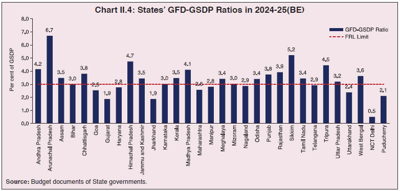
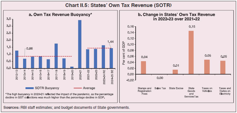
Sources: Budget documents of State governments; and Comptroller and Auditor General of India (CAG). | 2.6 States have budgeted for a GFD-GDP ratio of 3.2 per cent for 2024-25, a marginal increase from the level witnessed a year ago, with substantial inter-State variations (Chart II.4; Annex II.1). 3. Receipts 2.7 States’ revenue receipts (per cent of GDP) declined marginally in 2022-23, primarily due to lower tax devolution and grants-in-aid from the Centre (Table II.2). States registered a robust growth in their own tax revenue, driven by buoyant collections from stamp and registration fees, States’ goods and services tax (SGST), taxes on vehicles and taxes and duties on electricity.
2.8 The average buoyancy of own tax revenue of States increased to 1.44 in the post-pandemic period up from the pre-pandemic average of 0.86 during 2012-13 to 2019-20 (Chart II.5a). Revenue from sales tax and excise duties remained largely unchanged from the previous year (Chart II.5 b). The lower receipts under grants-in-aid from the Centre were mainly attributed to a decline in post-devolution revenue deficit grants. Non-tax revenue collections remained broadly stable in 2022-23. 2.9 In 2023-24, provisional accounts (PA) indicate that States’ revenue receipts moderated by 0.30 percentage points to 13.3 per cent of GDP, primarily due to a sharp dip in grants-in-aid from the Centre. Tax collections improved due to an increase in both own tax revenue and tax transfers from the Centre. Within States’ own tax revenues, SGST registered robust growth, supported by higher economic activity and improved compliance. States with a history of a low tax-GSDP ratios have witnessed considerable improvement in revenue mobilisation since the implementation of GST, leading to a reduction in inter-State disparities in tax collection (Box II.1). Sales tax collections remained muted. 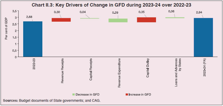
| Table II.2: Aggregate Receipts of State Governments and UTs | | (₹ lakh crore) | | Item | 2019-20 | 2020-21 | 2021-22 | 2022-23 | 2023-24
(RE) | 2023-24
(PA) | 2024-25
(BE) | | 1 | 2 | 3 | 4 | 5 | 6 | 7 | 8 | | 1. Revenue Receipts (a+b) | 26.7 | 25.9 | 32.3 | 36.5 | 42.1 | 39.2 | 46.7 | | | (13.3) | (13.0) | (13.7) | (13.6) | (14.3) | (13.3) | (14.3) | | a. States’ Own Revenue (i+ii) | 14.9 | 13.5 | 17.2 | 20.4 | 23.7 | - | 27.3 | | | (7.4) | (6.8) | (7.3) | (7.6) | (8.0) | - | (8.4) | | i. States’ Own Tax | 12.2 | 11.7 | 14.7 | 17.6 | 20.3 | - | 23.3 | | | (6.1) | (5.9) | (6.2) | (6.5) | (6.9) | - | (7.2) | | ii. States’ Own Non-Tax | 2.6 | 1.8 | 2.5 | 2.8 | 3.4 | 3.2 | 3.9 | | | (1.3) | (0.9) | (1.0) | (1.0) | (1.1) | (1.1) | (1.2) | | b. Central Transfers (i+ii) | 11.9 | 12.4 | 15.1 | 16.1 | 18.4 | - | 19.4 | | | (5.9) | (6.2) | (6.4) | (6.0) | (6.2) | - | (6.0) | | i. Shareable Taxes | 6.5 | 6.0 | 8.8 | 9.5 | 11.0 | - | 12.2 | | | (3.2) | (3.0) | (3.7) | (3.5) | (3.7) | - | (3.8) | | ii. Grants-in-Aid | 5.4 | 6.4 | 6.2 | 6.6 | 7.4 | 5.2 | 7.2 | | | (2.7) | (3.2) | (2.6) | (2.5) | (2.5) | (1.8) | (2.2) | | 2. Non-Debt Capital Receipts (i+ii) | 0.6 | 0.2 | 0.2 | 0.1 | 0.4 | 0.2 | 0.4 | | | (0.3) | (0.1) | (0.1) | (0.0) | (0.1) | (0.1) | (0.2) | | i. Recovery of Loans and Advances | 0.6 | 0.1 | 0.2 | 0.1 | 0.4 | 0.2 | 0.2 | | | (0.3) | (0.1) | (0.1) | (0.0) | (0.1) | (0.1) | (0.1) | | ii. Miscellaneous Capital Receipts | 0.0 | 0.1 | 0.0 | 0.0 | 0.0 | 0.0 | 0.2 | | | (0.0) | (0.0) | (0.0) | (0.0) | (0.0) | (0.0) | (0.1) | RE: Revised Estimates. PA: Provisional Accounts. BE: Budget Estimates.
Note: 1. Figures in parentheses are per cent of GDP.
2. ‘-’ : not available.
Sources: Budget documents of State governments; and CAG. |
Box II.1: GST and Convergence in the Tax-GSDP Ratios of States The introduction of the goods and services tax (GST) in India in 2017 simplified the indirect tax system by merging various State and Central taxes into a unified framework. It has played a crucial role in enhancing economic efficiency, benefiting consumers, and fostering sectoral growth (GoI, 2024). Statistical measures – Gini coefficient and coefficient of variation (CV) – show a decline in inter-State disparities in own tax-GSDP ratios after the implementation of GST (Chart 1). Beta-convergence is examined through a random-effects generalised least squares regression on a panel of 28 Indian States covering the period from 2001-02 to 2022-233 (Islam, 1995). The beta-convergence model tests whether States with initially lower ratios of SOTR-GSDP improved at a faster rate than those with higher ratios. The change in the SOTR-GSDP ratio is regressed on its initial level: yit–yi0 = α + β1 yi0 + β2 GST DUMMY + β3 GST DUMMY * yi0 + ui Where yi0 is SOTR-GSDP ratio of ith State in the initial time period (t=2001-02). Convergence is indicated if the coefficient of the initial level of SOTR-GSDP ratio (i.e., β1) is negative and statistically significant. An interaction variable is introduced to capture the impact of the GST reform.
| Table 1: Results of Beta-Convergence Test | | | Dependent Variable: Change in SOTR-GSDP ratio from initial base period | | Independent Variable | Coefficient | Standard error | Z-Value | | Initial SOTR-GSDP Ratio | -0.15*** | 0.64 | -2.33 | | GST Dummy | 2.54*** | 0.16 | 16.14 | | GST Dummy x Initial SOTR-GSDP Ratio (Interaction variable) | -0.47*** | 0.03 | -14.95 | | Intercept | 1.35*** | 0.32 | 4.24 | | Observations : 588 | Sigma_e : 0.66 | | | | Number of Groups : 28 | Rho : 0.47 | | | | R-squared (overall) : 0.3844 | Wald Chi2 (3) : 280.33 | | | | Sigma_u : 0.63 | | | | *** represent levels of significance at 1 per cent.
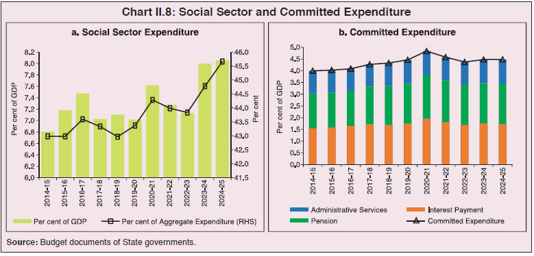
Source: RBI staff estimates. | The results indicate that GST positively impacted the growth of SOTR-GSDP ratios, particularly benefiting States with lower initial ratios (Table 1). The positive and statistically significant coefficient for the GST dummy suggests that GST improved tax performance across States. Moreover, the negative interaction term reveals that States with lower initial SOTR-GSDP ratios experienced stronger growth in tax revenues post-GST. The analysis thus suggests that GST has helped the low-performing States to catch up, fostering fiscal convergence in the post-GST period. Reference: Islam, N. (1995). “Growth Empirics: A Panel Data Approach”. The Quarterly Journal of Economics, 110(4), 1127-1170. GoI (2024). “Celebrating GST Day: A Milestone in Economic Reform”. July 4, 2024. https://pib.gov.in/PressNoteDetails.aspx?NoteId=151915&ModuleId=3®=3&lang=1. | 2.10 Non-tax revenues rose in 2023-24 on the back of higher collections from the renewal of existing mining leases and mining auctions. The sharp decline in grants from the Centre can be attributed to the cessation of GST compensation and the tapering of Finance Commission grants. 2.11 In 2024-25, the States have budgeted an increase in revenue receipts by 1 percentage point to 14.3 per cent of GDP, driven by both tax and non-tax sources. In the Union Budget, the devolution of States’ share in taxes is projected to grow by 10.4 per cent in 2024-25 (BE) over 2023-24 (PA). Within States’ own tax revenue, all major taxes – SGST, excise duties, and sales tax – are expected to increase (Chart II.6a). These key taxes account for over 75 per cent of total own tax revenue (Chart II.6b). 2.12 State governments are undertaking various initiatives to boost revenue collection, streamline compliance, and enhance transparency. Gujarat has established GST Seva Kendras to simplify registration and prevent documentation misuse, while Haryana plans to create facilitation cells to assist startups and MSMEs with GST compliance. Several States are leveraging technology to improve transparency. For instance, Haryana has implemented a QR code-based track-and-trace system to prevent diversion of alcohol, while Assam has implemented a similar system for its alcohol supply chain, alongside the introduction of e-tendering to ensure transparency in the issuances of wine licenses. Data analytics are being increasingly harnessed to track, monitor and simplify the refund process, with Delhi aiming to develop a faceless GST tax administration using data analytics and automation software, and Tamil Nadu and Karnataka using AI-driven analytics for real-time monitoring. Amnesty schemes have been introduced in States like Kerala and Rajasthan to waive penalties on tax arrears, aiding businesses for transition to the GST regime. States like Karnataka and Odisha are using advanced technologies, including drone surveys and satellite imaging, to monitor mining operations, prevent illegal activities, and enhance mining revenue.  2.13 The July 25, 2024 verdict given by the Supreme Court has granted States the authority to impose taxes on minerals and land containing minerals as well as to claim royalty payments retrospectively from April 1, 2005. These tax payments will be spread over 12 years starting from April 2026, with interest and penalties accrued before the judgment date being waived. This is likely to significantly benefit mineral-rich States such as Andhra Pradesh, Chhattisgarh, Jharkhand, Karnataka, Odisha, Madhya Pradesh, Maharashtra, Tamil Nadu, and Telangana. Jharkhand was the first State to levy taxes following the order, proposing a cess of ₹100 per tonne for coal and iron ore, ₹70 for bauxite, and ₹50 for manganese ore and other minerals. 4. Expenditure Revenue Expenditure 2.14 In 2022-23, States’ revenue expenditure (per cent of GDP) declined for the second consecutive year, falling close to its pre-pandemic ratio, with moderation in both developmental and non-developmental categories (Table II.3). 2.15 Within developmental expenditure, spending on medical and public health, natural calamity relief and the agriculture sector declined sharply with the ebbing of the pandemic, while that on housing and social security increased (Chart II.7a). The fall in non-developmental expenditure was mainly driven by lower outgoes on committed expenditure components like interest payments, administrative services, and pensions (Chart II.7b). 2.16 States’ revenue expenditure declined by a further 0.3 percentage points to 13.5 per cent of GDP in 2023-24 (PA). This declining trend is expected to reverse in 2024-25, with revenue expenditure budgeted to increase to 14.6 per cent of GDP. Social sector and committed expenditure are budgeted to remain broadly unchanged (Chart II.8a and II.8b). | Table II.3: Expenditure Pattern of State Governments and UTs | | (₹ lakh crore) | | Item | 2019-20 | 2020-21 | 2021-22 | 2022-23 | 2023-24
(RE) | 2023-24
(PA) | 2024-25
(BE) | | 1 | 2 | 3 | 4 | 5 | 6 | 7 | 8 | | Aggregate Expenditure (1+2 or 3+4+5) | 32.5 | 34.2 | 39.0 | 43.9 | 52.9 | 48.2 | 57.6 | | | (16.2) | (17.2) | (16.5) | (16.3) | (17.9) | (16.3) | (17.6) | | 1. Revenue Expenditure | 27.9 | 29.6 | 33.3 | 37.1 | 43.5 | 39.9 | 47.5 | | of which: | (13.9) | (14.9) | (14.1) | (13.8) | (14.7) | (13.5) | (14.6) | | Interest Payments | 3.5 | 3.9 | 4.3 | 4.6 | 5.2 | 4.7 | 5.6 | | | (1.8) | (2.0) | (1.8) | (1.7) | (1.8) | (1.6) | (1.7) | | 2. Capital Expenditure | 4.6 | 4.6 | 5.8 | 6.7 | 9.3 | 8.2 | 10.0 | | of which: | (2.3) | (2.3) | (2.4) | (2.5) | (3.2) | (2.8) | (3.1) | | Capital Outlay | 4.2 | 4.1 | 5.3 | 6.0 | 8.7 | 7.6 | 9.2 | | | (2.1) | (2.1) | (2.3) | (2.2) | (2.9) | (2.6) | (2.8) | | 3. Development Expenditure | 21.6 | 22.6 | 26.0 | 29.5 | 36.3 | - | 39.3 | | | (10.8) | (11.4) | (11.0) | (10.9) | (12.3) | - | (12.0) | | 4. Non-Development Expenditure | 10.1 | 10.6 | 12.0 | 13.3 | 15.3 | - | 16.9 | | | (5.0) | (5.4) | (5.1) | (4.9) | (5.2) | - | (5.2) | | 5. Others* | 0.8 | 0.9 | 1.0 | 1.1 | 1.3 | - | 1.4 | | | (0.4) | (0.4) | (0.4) | (0.4) | (0.4) | | (0.4) | RE: Revised Estimates. PA: Provisional Accounts. BE: Budget Estimates.
*: Includes grants-in-aid and contributions including compensation and assignments to local bodies.
Notes: 1. Figures in parentheses are per cent of GDP.
2. Capital expenditure includes capital outlay and loans and advances by the State governments.
3. ‘-’ : not available.
Sources: Budget documents of State governments; and CAG. | Capital Expenditure 2.17 States’ capital expenditure4 (per cent of GDP) increased marginally in 2022-23, primarily due to higher loans and advances extended by them for asset creation purposes. Capital outlays witnessed a marginal decline due to lower spending under economic services. Within developmental capital outlay, spending on water supply and sanitation, irrigation and flood control and energy fell, while allocations for urban and rural development increased (Chart II.9). 
 2.18 Capital expenditure increased to 2.8 per cent of GDP in 2023-24 (PA) from 2.5 per cent in 2022-23, facilitated inter alia by advance payment of tax devolution and enhanced allocation under the Centre’s scheme for Special Assistance to States for Capital Expenditure. The disbursement under the Centre’s scheme, which ranged between ₹11,000 – ₹15,000 crore in the initial two years of 2020-21 and 2021-22, surged to ₹81,195 crore in 2022-23 and further to ₹1,09,554 crore in 2023-24. These loans accounted for 14.4 per cent of the consolidated States’ capital outlay in 2023-24. Even after excluding these interest-free loans from the Centre, there has been a steady increase in capital outlays of the States since 2021-22 (Chart II.10).
2.19 The share of these loans in total capital outlay of States over the period 2022-23 to 2023-24 varied from 3.9 per cent (Odisha) to 50.6 per cent (Andhra Pradesh) (Chart II.11). 2.20 States’ have budgeted to increase their capital expenditure by another 0.3 percentage point to 3.1 per cent of GDP in 2024-25. Higher capital outlay has the tendency to increase medium-term growth prospects (Box II.2). Box II.2: Expenditure Multipliers of Indian States State governments have made commendable progress towards fiscal consolidation through higher revenue mobilisation and curtailment of revenue expenditure, while enhancing capital outlays. Although the moderation in revenue expenditure may have a negative impact on GDP growth in the short-term, the higher capital outlay is expected to boost economic growth in the medium term. The impact multiplier of revenue expenditure ranges between 0.60 and 1.74 (Jain and Kumar, 2013; Swaroop, 2022). Since its impact lasts for only one year, this is also the peak multiplier. In contrast, capital outlay has a long-lasting impact. Its impact multiplier is estimated between 2.13 and 2.71, with the peak multiplier ranging from 5.32 to 7.61. The net benefit of this trade-off depends on the relative size of the revenue expenditure and the capital outlay multiplier (Marjit et al., 2020). The revenue expenditure and capital outlay multipliers of States are estimated in a structural vector autoregressive (SVAR) model5 over the period from 1990-91 to 2023-24 with consolidated data of 31 States and Union Territories. In the SVAR model, the endogenous variables include the log differences of GDP, State government expenditure, and State government tax revenue. All the variables are taken in real terms. Exogenous variables such as the real call rate, output gap6 and global real growth account for monetary policy, economic conditions, and external factors, respectively. The model also includes dummy variables7 for GST reform, global financial crisis (2009-10), and the COVID year (2020-21). Following the methodology of Blanchard and Perotti (2002), the variables are ordered as government spending, GDP, and tax revenue, with a lower triangular matrix structure8. The results indicate that: (i) the cumulative revenue expenditure multipliers are almost a third of those for capital outlay (1.43 versus 3.84); (ii) the effects of revenue spending shocks last for only one year, while those of capital outlay shocks persist for a relatively longer period (5 years); and (iii) the multiplier values are broadly comparable with the ranges suggested in the literature (Table 1). Overall, the empirical analysis confirms the hypothesis that the short-term loss in growth from moderation in revenue expenditure is outweighed by the medium-term gains from higher capital outlay. | Table 1: Spending Multiplier* | | Government Expenditure Variable | Impact Multiplier | Peak Multiplier (Cumulative) | Peak Year | | Revenue Expenditure (less Interest Payment) | 1.43 | 1.43 | 1 | | Capital Outlay | 2.77 | 3.84 | 3 | *A value of ‘x’ for multiplier implies that an increase in expenditure of the government by ₹1 would raise the GDP by ₹‘x’.
Source: RBI staff estimates. | References Blanchard, O., and Perotti, R. (2002). “An Empirical Characterization of the Dynamic Effects of Changes in Government Spending and Taxes on Output”. Quarterly Journal of Economics. Vol. 117. pp. 1329–68. Jain, R., and Kumar, P. (2013). “Size of government expenditure multipliers in India: A structural VAR analysis”. RBI Working Paper No 7. Marjit, S., Sasmal, R. and Sasmal, J. (2020). “Composition of public expenditure and growth of per capita income in Indian states: a political perspective”. Journal of Social and Economic Development. 22. (1). 1-17. Swaroop, E. (2022). “Estimation of Expenditure Multiplier for India”. Working Paper. Retrieved from: https://www.ies.gov.in/working-paper.php | 2.21 With an increasing focus on capital expenditure, the ratio of revenue expenditure to capital outlay (RECO) of the States has seen a welcome decline from 6.3 in 2021-22 to 5.2 in 2024-25 (BE). There is, however, significant inter-state variation with the ratio moving in a range of 2.4 (Manipur) to 17.1 (Punjab) across States and exceeding 10 in some States in 2024-25 (BE) (Chart II.12). 2.22 The Union Budget for 2024-25 has increased allocation under the long-term interest-free loans to support States to ₹1.5 lakh crore in 2024-25 from ₹1.3 lakh crore in the previous year. Additionally, the Centre has proposed to introduce the Purvodaya plan aimed at all-round development of the eastern States – Bihar, Jharkhand, West Bengal, Odisha, and Andhra Pradesh. This initiative will focus on human resource development, infrastructure enhancement, and economic opportunity creation, with the goal of transforming the region into a significant driver of Viksit Bharat. The Centre will work with States and the private sector to develop ‘plug and play’ industrial parks equipped with complete infrastructure in or near 100 cities, using town planning schemes. States will be incentivised for advancing business reforms action plans and digitalisation efforts. Expenditure on Research and Development 2.23 Available data for 10 States and an UT9 indicate that their consolidated expenditure on research and development (R&D) is placed at around 0.1 per cent of GDP in the recent years (2022-23 to 2024-25), with wide spatial variations (Annex II.2). The R&D expenditures of States are primarily dominated by medical, health, family welfare, sanitation and agricultural research. Over time, the proportions of health and education related R&D spending have increased, while that of agricultural research has declined (Chart II.13).
5. Actual Outcome in 2024-25 So Far and Outlook 2.24 According to the provisional data for April-October 2024-25, States’ GFD increased to 54.6 per cent of BE from 48.7 per cent in the corresponding period of the previous year. The growth in tax revenues remained stable while there was a contraction in non-tax revenue and grants from the Centre (Chart II.14a). The pace of expansion in SGST – the largest driver of tax revenue – softened. While stamp and registration fees witnessed robust growth, sales tax displayed signs of recovery (Chart II.14b). 2.25 States’ revenue expenditure growth accelerated to 15.0 per cent during April-October 2024-25 (Chart II.15a). In contrast, capital expenditure declined during this period, mainly due to a high base effect and possibly reflecting the impact of the model code of conduct implemented during the general elections (Chart II.15a). Capital expenditure, however, showed signs of recovery in October 2024 (Chart II.15b).
2.26 States’ fiscal outlook remains favourable in view of resilient domestic economic activity, which is expected to support revenue buoyancy. On the expenditure side, States have contained the growth in revenue expenditure to 15.0 per cent during April-October 2024-25, below the full-year budget estimate of 19.2 per cent. Capital outlay of the States is expected to gain pace in the second half of the year, aided by the Centre’s 50-year interest free loans. 6. Financing of GFD and Market Borrowings by State Governments and UTs GFD Financing 2.27 On average, market borrowings financed slightly more than half of the consolidated gross fiscal deficit of States till 2016-17. States’ dependence on market borrowing has increased since then and is budgeted at 79 per cent in 2024-25, following the recommendation of the Fourteenth Finance Commission (FC-XIV) to exclude States from the National Small Saving Fund (NSSF) financing facility (barring Delhi, Madhya Pradesh, and Kerala). Market Borrowings 2.28 In 2023-24, the gross market borrowings of States and UTs surged by 32.8 per cent to ₹10.07 lakh crore, in line with their higher GFD (Chart II.16). 2.29 At a disaggregated level, all major States except Gujarat, Jharkhand, Madhya Pradesh, and Punjab saw an increase in market borrowings in 2023-24 (Table II.4). Chhattisgarh, Karnataka, Rajasthan, Goa, and Uttar Pradesh, which reduced their borrowings in the preceding two years, together contributed over 50 per cent of the incremental gross borrowings in 2023-24. There has been a consistent decline in market borrowings by Jharkhand over the past three years. North-Eastern and hilly States along with UTs contributed 5.9 per cent to the total gross borrowings. 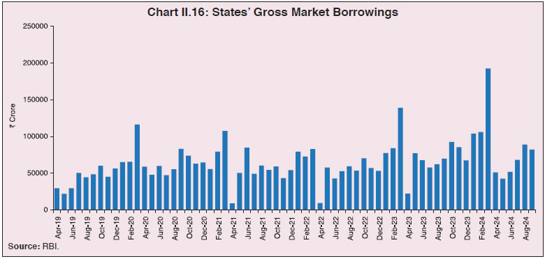 2.30 For 2024-25, States have budgeted gross market borrowings at ₹11.17 lakh crore. During April-September 2024, their gross market borrowings increased by 7.7 per cent over the same period last year, accounting for 35 per cent of the budget estimates. The consolidated actual borrowings by all the States generally remained lower than the indicative calendar (Chart II.17). States are expected to borrow ₹3.20 lakh crore in the quarter ending December 2024.
2.31 Net market borrowings of States rose by 38.2 per cent to ₹7.17 lakh crore in 2023-24, with Uttar Pradesh, Maharashtra, Tamil Nadu, Karnataka, Andhra Pradesh, Rajasthan, West Bengal and Telangana amongst the major borrowing States (Chart II.18 and Table II.5). 2.32 There were 782 issuances in 2023-24, of which 49 were re-issuances (6.3 per cent) as compared with 605 issuances in 2022-23 with 45 re-issuances (7.4 per cent). States such as Madhya Pradesh, Maharashtra, Puducherry, Punjab, Rajasthan, Tamil Nadu and Uttar Pradesh undertook re-issuances during the year. There were 16 re-issuances out of 329 total issuances during 2024-25 (April-September 2024). 2.33 State government securities (SGSs) with 10-year maturity accounted for 18.6 per cent of the total amount of issuances in 2023-24, down from 27.9 per cent in the previous year. The remaining 81.4 per cent was spread across maturities ranging between 2 and 40 years, and 57.6 per cent of outstanding SGSs were in the residual maturity bucket of five years and above (Table II.6 and Chart II.19a). | Table II.5: Market Borrowings of State Governments | | (₹ Crore) | | Item | 2020-21 | 2021-22 | 2022-23 | 2023-24 | 2024-25* | | 1 | 2 | 3 | 4 | 5 | 6 | | Maturities during the year | 1,47,039 | 2,09,143 | 2,39,562 | 2,89,918 | 3,19,965# | | Gross sanction under Article 293(3) | 9,69,525 | 8,95,166 | 8,80,779 | 11,29,295 | 6,99,396 | | Gross amount raised during the year | 7,98,816 | 7,01,626 | 7,58,392 | 10,07,058 | 3,85,636 | | Net amount raised during the year | 6,51,777 | 4,92,483 | 5,18,830 | 7,17,140 | 2,63,271 | | Amount raised during the year to total sanctions (per cent) | 82 | 78 | 86 | 89 | 44 | | Weighted average yield of SGSs (per cent) | 6.55 | 6.98 | 7.71 | 7.52 | 7.30 | | Weighted average spread over corresponding G-Sec (bps) | 53 | 41 | 31 | 31 | 31 | | Average inter-State spread (bps) | 10 | 4 | 3 | 3 | 2 | *: As at end-September 2024.
#: Data for maturity pertain to the full year.
Source: RBI. | 2.34 The weighted average cut-off yield (WAY) of SGSs fell to 7.52 per cent in 2023-24 from 7.71 per cent in the previous year (Chart II.19b). The weighted average spread (WAS) over comparable central government securities remained unchanged at 31 basis points, while the inter-State spread on 10-year tenor securities also stayed steady at 3 basis points (Table II.5). In H1:2024-25, yeilds softened due to both domestic and global factors. Financial Accommodation to States 2.35 Based on the recommendations made by the Group (consisting of select States Finance Secretaries) constituted by the Reserve Bank, the ways and means advances (WMA) limits of the State Governments/ UTs were revised up from July 01, 2024, to ₹60,118 crore from ₹47,010 crore. State governments/ UTs can avail overdraft (OD) for 14 consecutive days and can be in OD for a maximum number of 36 days in a quarter. During 2023-24, 15 States/UTs availed special drawing facility (SDF), 14 States/UTs resorted to WMA, and 11 States/UTs availed OD. 2.36 SDF availed by State governments/UTs shall continue to be linked to the quantum of their investments in marketable securities, issued by the central government, including auction treasury bills (ATBs). For investments held in ATBs, the maximum limit of SDF shall be 50 per cent of the lower of: (i) outstanding balance in ATBs (91/182/364 days) as on the last date of the second preceding quarter, and (ii) the current ATB balance. The maximum limit of SDF that can be availed by the States/ UTs against the investments held under Consolidated Sinking Fund (CSF)/ Guarantee Redemption Fund (GRF) shall be 50 per cent of the lower of: (i) outstanding balance of the funds as on the last date of the second preceding quarter, and (ii) the current balance held in CSF/ GRF. | Table II.6: Maturity Profile of Outstanding State Government Securities | | (As at end-March 2024) | | | (Per cent of Total Amount Outstanding) | | State/UT | less than 1Y | 1 to 5Y | 5 to 10Y | 10 to 20Y | Above 20Y | | 1 | 2 | 3 | 4 | 5 | 6 | | Andhra Pradesh | 5.6 | 25.0 | 27.8 | 41.7 | 0.0 | | Arunachal Pradesh | 4.6 | 53.4 | 42.0 | 0.0 | 0.0 | | Assam | 5.2 | 42.8 | 51.9 | 0.0 | 0.0 | | Bihar | 7.7 | 44.1 | 35.4 | 12.8 | 0.0 | | Chhattisgarh | 8.8 | 56.5 | 34.7 | 0.0 | 0.0 | | Goa | 4.1 | 48.9 | 43.2 | 3.8 | 0.0 | | Gujarat | 7.4 | 57.7 | 34.4 | 0.5 | 0.0 | | Haryana | 6.7 | 35.7 | 34.6 | 23.0 | 0.0 | | Himachal Pradesh | 4.8 | 33.9 | 35.4 | 25.8 | 0.0 | | Jammu and Kashmir | 2.4 | 38.0 | 20.2 | 23.5 | 15.9 | | Jharkhand | 9.5 | 43.8 | 35.4 | 11.3 | 0.0 | | Karnataka | 5.1 | 34.9 | 34.2 | 25.7 | 0.0 | | Kerala | 7.0 | 37.1 | 17.9 | 23.1 | 14.9 | | Madhya Pradesh | 7.1 | 32.6 | 25.1 | 33.4 | 1.8 | | Maharashtra | 6.4 | 37.0 | 48.7 | 8.0 | 0.0 | | Manipur | 4.4 | 42.4 | 39.7 | 13.5 | 0.0 | | Meghalaya | 7.2 | 54.3 | 32.9 | 5.7 | 0.0 | | Mizoram | 3.9 | 30.3 | 32.3 | 33.4 | 0.0 | | Nagaland | 4.5 | 37.1 | 58.5 | 0.0 | 0.0 | | Odisha | 18.3 | 39.6 | 23.8 | 18.3 | 0.0 | | Puducherry | 8.2 | 46.5 | 31.7 | 13.6 | 0.0 | | Punjab | 3.4 | 29.5 | 23.8 | 39.4 | 3.9 | | Rajasthan | 6.7 | 40.4 | 31.1 | 15.7 | 6.1 | | Sikkim | 3.1 | 39.5 | 57.4 | 0.0 | 0.0 | | Tamil Nadu | 5.5 | 34.1 | 29.2 | 11.5 | 19.7 | | Telangana | 4.4 | 20.2 | 14.0 | 38.0 | 23.5 | | Tripura | 1.6 | 75.2 | 7.3 | 15.9 | 0.0 | | Uttar Pradesh | 3.9 | 44.3 | 41.3 | 10.6 | 0.0 | | Uttarakhand | 4.9 | 58.3 | 36.7 | 0.0 | 0.0 | | West Bengal | 4.6 | 29.4 | 23.1 | 42.4 | 0.5 | | All States and UTs | 5.7 | 36.7 | 31.8 | 20.8 | 5.0 | | Source: RBI. |
 Cash Management of State Governments 2.37 As on March 31, 2024, States/UTs on an aggregate basis maintained a surplus cash balance that was invested in intermediate treasury bills (ITBs) and ATBs (Table II.7). Although positive cash balances indicate low intra-year fiscal pressure, they involve a negative cost of carry. States’ Reserve Funds 2.38 Given the increasing borrowing requirements by the States and mounting contingent liabilities, it is desirable to keep adequate buffers to minimise the potential fiscal stress that could arise from redemption pressures and unforeseen liabilities. State governments maintain the CSF and GRF with the Reserve Bank as a buffer for repayment of their future liabilities. States can also avail SDF at a discounted rate from the Reserve Bank against funds invested in CSF and GRF. So far, 25 States and two UTs, i.e., Jammu and Kashmir and Puducherry, have set up CSF. Similarly, 20 States and the UT of Jammu and Kashmir are currently members of GRF (Table II.8). Outstanding investments in CSF and GRF stood at ₹2,06,441 crore and ₹12,259 crore, respectively, at end-March 2024, as against ₹1,84,029 crore and ₹10,839 crore, respectively, at end-March 2023. | Table II.7: State Governments’ Investments in Treasury Bills | | (Outstanding as on March 31) | | (₹ Crore) | | Item | 2020 | 2021 | 2022 | 2023 | 2024 | | 1 | 2 | 3 | 4 | 5 | 6 | | 14-Day (ITBs) | 1,54,757 | 2,05,230 | 2,16,272 | 2,12,758 | 2,66,805 | | ATBs | 33,504 | 41,293 | 87,400 | 58,913 | 51,258 | | Total | 1,88,261 | 2,46,523 | 3,03,672 | 2,71,671 | 3,18,063 | | Source: RBI. |
| Table II.8: Investment in CSF/GRF by States/UTs (March 31, 2024) | | (₹ Crore) | | State/UT | CSF | GRF | CSF as per cent of Outstanding Liabilities | | 1 | 2 | 3 | 4 | | Andhra Pradesh | 10,901 | 1,072 | 2.2 | | Arunachal Pradesh | 2,495 | 6.0 | 11.4 | | Assam | 5,881 | 85 | 3.8 | | Bihar | 10,279 | - | 3.1 | | Chhattisgarh | 7,323 | 15.0 | 5.1 | | Goa | 926 | 431 | 2.8 | | Gujarat | 12,549 | 628 | 2.8 | | Haryana | 2,206 | 1,608 | 0.7 | | Himachal Pradesh | - | - | - | | Jammu & Kashmir | - | - | - | | Jharkhand | 1,691 | - | 1.4 | | Karnataka | 17,288 | 518 | 2.7 | | Kerala | 2,934 | - | 0.7 | | Madhya Pradesh | - | 1,202 | - | | Maharashtra | 65,876 | 1,648 | 8.9 | | Manipur | 65.0 | 132 | 0.4 | | Meghalaya | 1,200 | 102 | 5.7 | | Mizoram | 432 | 60 | 3.4 | | Nagaland | 1,681 | 44 | 9.0 | | Odisha | 17,136 | 1,927 | 12.6 | | Puducherry | 547 | - | 4.2 | | Punjab | 8,637 | - | 2.5 | | Rajasthan | - | - | - | | Tamil Nadu | 3,226 | - | 0.4 | | Telangana | 7,453 | 1,630 | 1.9 | | Tripura | 1,154 | 25 | 4.9 | | Uttar Pradesh | 7,687 | - | 1.0 | | Uttarakhand | 4,726 | 199 | 5.5 | | West Bengal | 12,211 | 926 | 1.9 | | Total | 2,06,441 | 12,259 | 2.5 | ‘-’ : Indicates no fund is maintained.
Note.: 1. UT of J&K became a member to CSF/GRF post March 31, 2024.
2. Rajasthan became a member to CSF post March 31, 2024.
3. Total may not add due to rounding off.
Source: RBI. | 7. Outstanding Liabilities 2.39 States’ total outstanding liabilities declined to 28.2 per cent of GDP by end-March 2023 from the pandemic peak of 31 per cent at end-March 2021, driven by sustained fiscal consolidation (Table II.9). The ratio is, however, budgeted to increase marginally to 28.8 per cent by end-March 2025. | Table II.9: Outstanding Liabilities of State Governments and UTs | | Year | Amount | Annual Growth | Debt /GDP | | (End-March) | (₹ lakh crore) | (Per cent) | | 1 | 2 | 3 | 4 | | 2016 | 32.59 | 18.8 | 23.7 | | 2017 | 38.59 | 18.4 | 25.1 | | 2018 | 42.92 | 11.2 | 25.1 | | 2019 | 47.87 | 11.5 | 25.3 | | 2020 | 53.51 | 11.8 | 26.6 | | 2021 | 61.55 | 15.0 | 31.0 | | 2022 | 68.76 | 11.7 | 29.1 | | 2023 | 75.93 | 10.4 | 28.2 | | 2024 (RE) | 84.20 | 10.9 | 28.5 | | 2025 (BE) | 93.93 | 11.6 | 28.8 | RE: Revised Estimates. BE: Budget Estimates.
Sources: 1. Budget documents of State governments.
2. Combined finance and revenue accounts of the Union and the State governments in India, Comptroller and Auditor General (CAG) of India.
3. Ministry of Finance, Government of India.
4. Reserve Bank records.
5. Finance accounts of the Union government, Government of India. |
2.40 At a disaggregated level, the debt-GSDP ratio is budgeted higher than 25 per cent10 for 26 States and UTs at end-March 2025 (Statement 20 and Chart II.20). 2.41 The debt-service ratio, measured by the interest payment to revenue receipts (IP-RR), has been declining gradually since 2020-21 (Chart II.21). 2.42 The share of market borrowings in total outstanding liabilities is budgeted to rise to 68.8 per cent by end-March 2025 (Table II.10). Similarly, the share of loans from the Centre is budgeted to increase to 8.9 per cent by end-March 2025 from 3 per cent at end-March 2020, primarily due to back-to-back loans in lieu of GST compensation and 50-year interest-free loans under the scheme for ‘Special Assistance to the States for Capital Expenditure’. On the other hand, the shares of the NSSF, loans from banks and financial institutions, and public accounts in total outstanding liabilities have decreased over time. 
| Table II.10: Composition of Outstanding Liabilities of State Governments and UTs | | (As at end-March) | | (Per cent) | | Item | 2019 | 2020 | 2021 | 2022 | 2023 | 2024 RE | 2025 BE | | 1 | 2 | 3 | 4 | 5 | 6 | 7 | 8 | | Total Liabilities (1 to 4) | 100.0 | 100.0 | 100.0 | 100.0 | 100.0 | 100.0 | 100.0 | | 1. Internal Debt | 72.2 | 73.5 | 74.0 | 73.0 | 72.5 | 73.7 | 74.5 | | of which: | | | | | | | | | (i) Market Loans | 58.0 | 61.0 | 63.7 | 64.1 | 64.9 | 67.1 | 68.8 | | (ii) Special Securities Issued to NSSF | 9.2 | 7.7 | 6.1 | 5.1 | 4.1 | 3.3 | 2.6 | | (iii) Loans from Banks and Financial Institutions | 4.8 | 4.8 | 4.2 | 3.8 | 3.5 | 3.7 | 3.7 | | 2. Loans and Advances from the Centre | 3.6 | 3.0 | 5.1 | 7.2 | 7.7 | 8.3 | 8.9 | | 3. Public Account (i to iii) | 24.1 | 23.4 | 20.8 | 19.7 | 19.7 | 17.9 | 16.5 | | (i) State PF, etc. | 10.2 | 9.8 | 8.8 | 8.4 | 7.9 | 7.5 | 7.1 | | (ii) Reserve Funds | 4.2 | 3.8 | 3.4 | 3.4 | 3.8 | 3.4 | 3.1 | | (iii) Deposits & Advances | 9.7 | 9.7 | 8.6 | 7.9 | 8.0 | 6.9 | 6.3 | | 4. Contingency Fund | 0.1 | 0.1 | 0.1 | 0.1 | 0.1 | 0.1 | 0.1 | RE: Revised Estimate. BE: Budget Estimate.
Sources: 1. Budget documents of State governments.
2. Combined finance and revenue accounts of the Union and the State governments in India, Comptroller and Auditor General (CAG) of India.
3. Ministry of Finance, Government of India.
4. Reserve Bank records.
5. Finance accounts of the Union government, Government of India. | Contingent Liabilities 2.43 Outstanding guarantees of States increased from 2 per cent of GDP at end-March 2017 to 3.9 per cent at end-March 2021, with a marginal dip to 3.8 per cent at end-March 2023 (Table II.11). Data from 20 States and UTs indicate that outstanding guarantees increased by 10.6 per cent by end-March 2024. States need to put in place a robust system of monitoring and reporting of guarantees to avoid unforeseen fiscal stress. In line with the recommendations of the Working Group on State Government Guarantees (2024), States may adopt ceilings on guarantees and strengthen frameworks for their management (Box II.3). | Table II.11: Guarantees Issued by State Governments | | Year (End-March) | Guarantees Outstanding | | ₹ lakh crore | As per cent of GDP | | 1 | 2 | 3 | | 2015 | 4.28 | 3.4 | | 2016 | 3.64 | 2.6 | | 2017 | 3.12 | 2.0 | | 2018 | 4.29 | 2.5 | | 2019 | 5.38 | 2.8 | | 2020 | 6.33 | 3.1 | | 2021 | 7.79 | 3.9 | | 2022 | 9.21 | 3.9 | | 2023 | 10.31 | 3.8 | | Sources: State governments; and CAG. |
Box II.3: Working Group on State Government Guarantees – Major Recommendations Government guarantee is a potential future liability contingent upon the occurrence of an unforeseen future event. If these liabilities get crystallised without adequate buffer, it would lead to increase in expenditure, budgetary deficits, and debt levels for the issuing government. In view of such risks, the 32nd Conference of the State Finance Secretaries held on July 7, 2022 set up a Working Group comprising members from the Ministry of Finance, Government of India; Comptroller and Auditor General of India; and select State governments to review the framework of State government guarantees. The major recommendations of the report of the Working Group, placed on the Reserve Bank’s website on January 16, 2024, are: -
No distinction should be made between conditional/ unconditional/ financial/ performance guarantees as far as assessment of fiscal risk is concerned as all of these are contingent liabilities that might get crystallised on a future date. -
The word ‘guarantee’ should be used in a broader sense and may include instruments by whatever name they are called if they create obligations on the part of the guarantor (State government) for making payment on behalf of the borrower (State enterprise) at a future date, contingent or otherwise. -
State governments may be guided by the broad guidelines issued by the Government of India (GoI, 2022)11 while formulating their own guarantee policy. -
The purpose for which government guarantees may be issued should be clearly defined in line with Rule 276 of General Financial Rules, 201712. Government guarantees should, however, not be used to obtain finance through State owned entities. Government guarantees should not be allowed for creating direct liability/de-facto liability on the State. -
States should classify projects/ activities as high, medium and low-risk and assign appropriate risk weights before extending guarantees. Such risk categorisation should also take into consideration past records of defaults. -
The ceiling for incremental guarantees issued during a year should be 5 per cent of revenue receipts or 0.5 per cent of GSDP, whichever is less. -
The guarantee fee charged should reflect the riskiness of the borrowers / projects / activities. A minimum of 0.25 per cent per annum may be considered as the base or minimum guarantee fee. Additional risk premium, based on risk assessment by the State government, may be charged to each risk category of issuances. The guarantee fee should also be linked to the tenor of the underlying loan. -
States which are currently not members of the guarantee redemption fund (GRF) should consider becoming members at the earliest. -
States should continue with their contributions towards building up the GRF to a desirable level of five per cent of their total outstanding guarantees over a period of five years from the date of constitution of the fund. The corpus may be maintained on a rolling basis thereafter. -
The borrowing state enterprises should set up escrow accounts with pre-determined and regular contributions from project earnings. In case revenue from the project suffers for any reason, repayments could be made from these accounts before resorting to State government guarantees. -
A unit responsible for tracking all the guarantees may be designated at the State level (preferably, within the Department of Finance). The unit would be responsible for compilation, consolidation, maintenance of the database on guarantees and monitoring the same on a continuous basis. -
To ensure uniformity and consistency, the State governments may publish/ disclose data relating to guarantees as per the Indian Government Accounting Standard recommended by Government of India13. Reference RBI (2024). “Working Group on State Government Guarantees”. | 8. Conclusion 2.44 State governments have made commendable progress towards fiscal consolidation by containing their aggregate gross fiscal deficit within 3 per cent of GDP for three consecutive years (2021-22 to 2023-24), while restricting revenue deficit at 0.2 per cent of GDP in 2022-23 and 2023-24. This has allowed the States to scale up their capital spending and improve the quality of expenditure. However, the RECO ratio exceeds 10 in some States, constraining their scope for capital expenditure. 2.45 Several States have announced sops pertaining to farm loan waiver, free electricity to agriculture and households, free transport, allowances to unemployed youth and monetary assistance to women in their Budget for 2024-25. Such spending could crowd out the resources available with them and hamper their capacity to build critical social and economic infrastructure. High debt-GDP ratio, outstanding guarantees and the increasing subsidy burden require States to persevere with fiscal consolidation while laying greater emphasis on developmental and capital spending.
| Annex II.1: Deficit Indicators - State-wise | | (Per cent of GSDP) | | State/UT | GFD | RD | PD | | 2022-23 | 2023-24
(RE) | 2024-25
(BE) | 2022-23 | 2023-24
(RE) | 2024-25
(BE) | 2022-23 | 2023-24
(RE) | 2024-25
(BE) | | 1 | 2 | 3 | 4 | 5 | 6 | 7 | 8 | 9 | 10 | | 1. Andhra Pradesh | 4.0 | 4.4 | 4.2 | 3.3 | 2.7 | 2.1 | 2.1 | 2.3 | 2.5 | | 2. Arunachal Pradesh | 5.0 | 9.6 | 6.7 | -18.1 | -14.7 | -11.9 | 2.6 | 7.3 | 4.6 | | 3. Assam | 5.9 | 5.2 | 3.5 | 2.5 | 0.2 | -0.3 | 4.5 | 3.7 | 2.0 | | 4. Bihar | 6.0 | 8.9 | 3.0 | 1.5 | 4.2 | -0.1 | 4.0 | 6.8 | 0.9 | | 5. Chhattisgarh | 1.0 | 7.3 | 3.8 | -1.9 | 3.1 | -0.2 | -0.4 | 5.9 | 2.4 | | 6. Goa | 1.2 | 3.9 | 2.5 | -2.7 | -0.9 | -1.6 | -0.9 | 1.9 | 0.8 | | 7. Gujarat | 0.8 | 1.7 | 1.9 | -0.9 | -0.8 | -0.4 | -0.4 | 0.6 | 0.8 | | 8. Haryana | 3.2 | 2.8 | 2.8 | 1.7 | 1.2 | 1.5 | 1.1 | 0.8 | 0.7 | | 9. Himachal Pradesh | 6.5 | 6.1 | 4.7 | 3.3 | 2.8 | 2.0 | 3.9 | 3.4 | 2.0 | | 10. Jammu and Kashmir | 2.2 | 5.9 | 3.5 | -2.7 | -3.1 | -6.3 | -1.7 | 2.0 | -0.5 | | 11. Jharkhand | 1.1 | 2.5 | 1.9 | -3.2 | -1.5 | -3.7 | -0.4 | 0.9 | 0.5 | | 12. Karnataka | 2.1 | 2.7 | 3.0 | -0.6 | 0.6 | 1.0 | 0.8 | 1.5 | 1.6 | | 13. Kerala | 2.5 | 3.5 | 3.5 | 0.9 | 2.1 | 2.2 | 0.0 | 1.2 | 1.2 | | 14. Madhya Pradesh | 3.3 | 4.0 | 4.1 | -0.3 | 0.0 | -0.1 | 1.7 | 2.2 | 2.3 | | 15. Maharashtra | 1.9 | 2.8 | 2.6 | 0.1 | 0.5 | 0.5 | 0.7 | 1.6 | 1.3 | | 16. Manipur | 4.4 | 4.5 | 2.8 | -4.3 | -10.2 | -13.1 | 2.2 | 2.6 | 0.8 | | 17. Meghalaya | 6.0 | 3.5 | 3.4 | 0.1 | -7.3 | -6.5 | 3.8 | 1.3 | 1.3 | | 18. Mizoram | 3.6 | 5.2 | 3.0 | -0.6 | -0.6 | -1.3 | 2.0 | 3.4 | 1.7 | | 19. Nagaland | 4.2 | 5.8 | 2.9 | -1.9 | -0.9 | -2.3 | 1.5 | 3.1 | 0.2 | | 20. Odisha | 2.0 | 2.9 | 3.4 | -2.6 | -2.6 | -2.9 | 1.3 | 2.1 | 2.8 | | 21. Punjab | 5.0 | 4.1 | 3.8 | 3.8 | 3.2 | 2.9 | 2.1 | 1.0 | 0.8 | | 22. Rajasthan | 3.8 | 4.3 | 3.9 | 2.3 | 2.0 | 1.4 | 1.5 | 2.0 | 1.8 | | 23. Sikkim | 4.5 | 5.2 | 5.2 | -1.1 | -1.9 | -0.9 | 2.8 | 3.5 | 3.5 | | 24. Tamil Nadu | 3.4 | 3.5 | 3.4 | 1.5 | 1.7 | 1.6 | 1.5 | 1.4 | 1.5 | | 25. Telangana | 2.5 | 3.3 | 2.9 | -0.5 | -0.1 | 0.0 | 0.8 | 1.7 | 1.9 | | 26. Tripura | 2.1 | 4.1 | 4.5 | -0.8 | -1.3 | -1.9 | 0.2 | 2.4 | 2.9 | | 27. Uttar Pradesh | 2.8 | 3.2 | 3.2 | -1.6 | -2.8 | -2.7 | 0.9 | 1.3 | 1.2 | | 28. Uttarakhand | 1.0 | 2.2 | 2.4 | -1.7 | -0.9 | -1.2 | -0.7 | 0.4 | 0.7 | | 29. West Bengal | 3.3 | 3.5 | 3.6 | 1.8 | 1.7 | 1.7 | 0.6 | 1.0 | 1.2 | | 30. NCT Delhi | -0.4 | 0.7 | 0.5 | -1.4 | -0.4 | -0.3 | -0.8 | 0.4 | 0.3 | | 31. Puducherry | -0.8 | 1.6 | 2.1 | -1.5 | 0.4 | 0.6 | -2.5 | -0.1 | 0.6 | | All States and UTs | 2.7 | 3.5 | 3.2 | 0.2 | 0.5 | 0.2 | 1.0 | 1.8 | 1.5 | RE: Revised Estimates. BE: Budget Estimates. RD: Revenue Deficit. GFD: Gross Fiscal Deficit. PD: Primary Deficit.
Note: Negative (-) sign in deficit indicators indicates surplus.
Source: Budget documents of State governments. |
| Annex II.2: States’ Expenditure on Research and Development (R&D) | | (₹ Crore) | | Item | 2020-21 | 2021-22 | 2022-23 | 2023-24
(RE) | 2024-25
(BE) | | 1 | 2 | 3 | 4 | 5 | 6 | | Andhra Pradesh | | Total R&D (a to g) | 143.1 | 98.8 | 23.5 | 45.7 | – | | | (0.01) | (0.01) | (0.00) | (0.00) | – | | a. Education | 2.9 | 3.4 | 5.2 | 4.8 | – | | b. Medical, Health, Family Welfare and Sanitation | – | 10.7 | 13.9 | 35.0 | – | | c. Agricultural Research | – | – | 1.0 | 0.4 | – | | d. Industrial Research | 135.6 | 79.8 | – | – | – | | e. Environmental Research | 2.97 | 3.5 | 1.6 | 3.5 | – | | f. Infrastructure Research | 1.7 | 1.5 | 1.8 | 2.0 | – | | g. Others | – | – | – | – | – | | Bihar | | Total R&D (a to g) | 15.3 | 30.5 | 6.6 | 8.5 | 7.0 | | | (0.00) | (0.00) | (0.00) | (0.00) | (0.00) | | a. Education | – | – | – | – | – | | b. Medical, Health, Family Welfare and Sanitation | – | – | 5.2 | 5.7 | 6.2 | | c. Agricultural Research | 2.0 | 1.4 | – | – | – | | d. Industrial Research | – | – | – | – | – | | e. Environmental Research | – | – | 0.0 | 0.1 | 0.1 | | f. Infrastructure Research | – | – | – | – | – | | g. Others | 13.3 | 29.1 | 1.4 | 2.7 | 0.7 | | Haryana | | Total R&D (a to g) | 561.8 | 647.2 | 729.8 | 808.3 | 351.1 | | | (0.08) | (0.07) | (0.07) | (0.07) | (0.03) | | a. Education | 13.0 | 14.6 | 25.7 | 29.3 | 7.6 | | b. Medical, Health, Family Welfare and Sanitation | 0.8 | 1.0 | 0.4 | 0.6 | 0.1 | | c. Agricultural Research | 504.9 | 602.4 | 666.9 | 631.8 | 313.4 | | d. Industrial Research | – | – | – | – | – | | e. Environmental Research | 3.7 | 5.7 | 2.9 | 0.7 | 0.5 | | f. Infrastructure Research | 38.7 | 22.3 | 28.9 | 134.8 | 9.5 | | g. Others | 0.8 | 1.2 | 5.1 | 11.2 | 20.0 | | Karnataka | | Total R&D (a to g) | 1798.7 | 1826.9 | 1769.8 | 2106.9 | 2057.5 | | | (0.11) | (0.09) | (0.08) | (0.08) | (0.07) | | a. Education | 40.5 | 41.5 | 46.8 | 53.3 | 51.3 | | b. Medical, Health, Family Welfare and Sanitation | 636.4 | 647.4 | 768.3 | 975.7 | 945.1 | | c. Agricultural Research | 652.4 | 647.3 | 573.5 | 641.1 | 601.1 | | d. Industrial Research | 4.6 | 4.8 | 0.9 | 0.8 | 0.5 | | e. Environmental Research | 62.9 | 59.8 | 21.7 | 18.5 | 18.3 | | f. Infrastructure Research | – | – | – | – | – | | g. Others | 401.8 | 426.2 | 358.5 | 417.7 | 441.2 | | Kerala | | Total R&D (a to g) | – | – | – | 3482.4 | 3678.5 | | | – | – | – | (0.30) | (0.28) | | a. Education | – | – | – | 1611.7 | 1706.4 | | b. Medical, Health, Family Welfare and Sanitation | – | – | – | 802.1 | 871.0 | | c. Agricultural Research | – | – | – | 510.1 | 541.0 | | d. Industrial Research | – | – | – | 276.2 | 344.4 | | e. Environmental Research | – | – | – | 19.4 | 14.3 | | f. Infrastructure Research | – | – | – | 56.1 | 64.6 | | g. Others | – | – | – | 206.9 | 136.8 | | Madhya Pradesh | | Total R&D (a to g) | – | – | – | – | 8.0 | | | – | – | – | – | (0.00) | | a. Education | – | – | – | – | – | | b. Medical, Health, Family Welfare and Sanitation | – | – | – | – | – | | c. Agricultural Research | – | – | – | – | 8.0 | | d. Industrial Research | – | – | – | – | – | | e. Environmental Research | – | – | – | – | – | | f. Infrastructure Research | – | – | – | – | – | | g. Others | – | – | – | – | – | | Meghalaya | | Total R&D (a to g) | 77.8 | 150.7 | 103.1 | 103.3 | 123.5 | | | (0.23) | (0.39) | (0.24) | (0.22) | (0.23) | | a. Education | 37.0 | 97.2 | 63.1 | 59.4 | 65.3 | | b. Medical, Health, Family Welfare and Sanitation | 0.1 | 5.3 | 3.9 | 0.0 | 0.0 | | c. Agricultural Research | 29.8 | 38.4 | 30.3 | 33.6 | 38.1 | | d. Industrial Research | – | – | – | – | – | | e. Environmental Research | 0.7 | 0.0 | 0.0 | 0.0 | 0.0 | | f. Infrastructure Research | 10.1 | 3.5 | 4.8 | 0.0 | 0.0 | | g. Others | 0.0 | 6.4 | 1.1 | 10.3 | 20.1 | | Nagaland | | Total R&D (a to g) | 30.6 | 32.8 | 30.4 | 38.0 | 39.7 | | | (0.10) | (0.10) | (0.09) | (0.08) | (0.08) | | a. Education | 10.3 | 11.4 | 10.2 | 11.3 | 11.4 | | b. Medical, Health, Family Welfare and Sanitation | 1.7 | 2.0 | 3.0 | 2.4 | 2.4 | | c. Agricultural Research | 14.8 | 13.7 | 11.5 | 19.6 | 20.2 | | d. Industrial Research | 0.0 | 0.0 | 0.0 | 0.0 | 0.0 | | e. Environmental Research | 0.0 | 0.1 | 0.1 | 0.0 | 0.0 | | f. Infrastructure Research | 2.2 | 2.3 | 2.7 | 2.8 | 3.0 | | g. Others | 1.6 | 3.3 | 3.0 | 2.0 | 2.8 | | Odisha | | Total R&D (a to g) | 388.8 | 550.7 | 879.4 | 1900.0 | 2294.9 | | | (0.02) | (0.03) | (0.04) | (0.10) | (0.12) | | a. Education | 125.5 | 195.3 | 296.7 | 853.3 | 1142.1 | | b. Medical, Health, Family Welfare and Sanitation | 25.7 | 29.8 | 69.2 | 113.8 | 110.0 | | c. Agricultural Research | 24.6 | 96.6 | 123.8 | 229.5 | 220.4 | | d. Industrial Research | 2.3 | 2.0 | 3.1 | 13.7 | 97.2 | | e. Environmental Research | 15.6 | 12.9 | 29.8 | 37.4 | 67.4 | | f. Infrastructure Research | 38.8 | 56.9 | 79.4 | 240.3 | 169.8 | | g. Others | 156.3 | 157.3 | 277.5 | 411.9 | 488.1 | | Puducherry | | Total R&D (a to g) | 1.64 | 2.08 | 1.73 | 1.56 | 1.97 | | | (0.00) | (0.00) | (0.00) | (0.00) | (0.00) | | a. Education | 0.3 | 0.3 | 0.2 | 0.1 | 0.0 | | b. Medical, Health, Family Welfare and Sanitation | 0.0 | 0.0 | – | – | – | | c. Agricultural Research | 0.0 | 0.0 | – | – | – | | d. Industrial Research | 0.0 | 0.0 | – | – | – | | e. Environmental Research | 0.0 | 0.0 | – | – | – | | f. Infrastructure Research | 0.0 | 0.0 | 0.1 | 0.0 | 0.1 | | g. Others | 1.3 | 1.8 | 1.4 | 1.4 | 1.9 | | Punjab | | Total R&D (a to g) | 499.8 | 520.8 | 546.3 | 591.2 | 879.4 | | | (0.09) | (0.08) | (0.08) | (0.08) | (0.11) | | a. Education | 83.9 | 102.2 | 112.6 | 89.8 | 425.1 | | b. Medical, Health, Family Welfare and Sanitation | 0.0 | 0.6 | 0.3 | 0.7 | 1.1 | | c. Agricultural Research | 397.9 | 403.8 | 414.5 | 489.1 | 436.6 | | d. Industrial Research | - | 0.0 | 0.7 | 0.3 | 0.6 | | e. Environmental Research | 2.9 | 4.3 | 4.5 | 3.8 | 6.8 | | f. Infrastructure Research | - | - | 0.0 | - | - | | g. Others | 15.1 | 9.9 | 13.6 | 7.5 | 9.2 | | Rajasthan | | Total R&D (a to g) | 2831.6 | 3554.8 | 5109.2 | 6422.4 | 7488.2 | | | (0.28) | (0.29) | (0.38) | (0.42) | (0.42) | | a. Education | 20.9 | 16.8 | 52.3 | 59.4 | 83.0 | | b. Medical, Health, Family Welfare and Sanitation | 1977.5 | 2571.8 | 4012.2 | 4973.7 | 5773.9 | | c. Agricultural Research | 309.8 | 318.6 | 393.6 | 460.1 | 417.2 | | d. Industrial Research | 0.0 | 0.2 | 0.8 | 0.3 | 0.3 | | e. Environmental Research | 3.2 | 5.0 | 8.0 | 3.4 | 5.7 | | f. Infrastructure Research | 182.0 | 214.9 | 213.2 | 210.2 | 447.4 | | g. Others | 338.1 | 427.4 | 429.1 | 715.2 | 760.8 | | Tamil Nadu | | Total R&D (a to g) | 530.2 | 428.0 | 391.0 | 311.6 | 350.2 | | | (0.03) | (0.02) | (0.02) | (0.01) | (0.01) | | a. Education | 11.0 | 8.8 | 11.5 | 67.6 | 76.5 | | b. Medical, Health, Family Welfare and Sanitation | 4.6 | 4.4 | 4.6 | 4.9 | 5.2 | | c. Agricultural Research | 425.2 | 331.7 | 261.9 | 112.4 | 137.9 | | d. Industrial Research | 1.7 | 1.5 | 9.4 | 2.3 | 1.5 | | e. Environmental Research | 7.3 | 9.4 | 10.0 | 13.5 | 11.8 | | f. Infrastructure Research | 70.2 | 61.7 | 83.1 | 95.7 | 103.5 | | g. Others | 10.1 | 10.5 | 10.7 | 15.4 | 13.8 | | West Bengal | | Total R&D (a to g) | 151.4 | 156.1 | 128.4 | 168.4 | 198.1 | | | (0.01) | (0.01) | (0.01) | (0.01) | (0.01) | | a. Education | 1.8 | 1.9 | 1.3 | 2.1 | 6.0 | | b. Medical, Health, Family Welfare and Sanitation | 4.7 | 3.3 | 3.7 | 6.3 | 7.1 | | c. Agricultural Research | 117.8 | 115.2 | 103.8 | 110.6 | 117.2 | | d. Industrial Research | 6.4 | 13.6 | 10.7 | 20.2 | 34.8 | | e. Environmental Research | 3.0 | 3.3 | -7.8 | 3.0 | 6.7 | | f. Infrastructure Research | 5.4 | 6.1 | 5.6 | 12.3 | 9.8 | | g. Others | 12.4 | 12.8 | 11.3 | 14.0 | 16.5 | ‘-’: Not available.
Note: Figures in parentheses are per cent of GSDP.
Source: State governments. |
|