Janak Raj and Sarat Dhal¹

Abstract

This study addresses some applied issues pertaining to the two alternative indicators of wholesale price inflation rate, i.e. the month-over-month inflation rate and the year-on-year or the annual inflation rate in the Indian context. Based on various empirical exercises pertaining to the relationship of inflation with money, output growth, interest rate and asset price variation, the study finds evidence that the standard year-on-year inflation rate could be more meaningful than the monthly inflation rate.

JEL Classification : E31, E310
Keywords             :  Inflation, Price Level.

Introduction

Economists’ interest on how to construct the appropriate aggregate price index and measure the inflation rate has the history of a century long period. Over this period, paradigm shifts are evident from the literature moving across the spectrum of views. The early literature shows that Irving Fisher (1906) was in favour of a broad transaction price metric or the aggregate price index, comprising prices of goods, services and assets in order to reflect on the price level as implied by the broader equation of exchange and guide the authorities in determining the price of monetary unit. However, Fisher maintained that the appropriateness of any price index could be contextual; different problems necessitating different indices due to differences in the comparative places or comparative times under investigation (Bryan, et.al. 2002). Deriving from Fisher (1906) and Samuelson (1961), Alchian and Klein (1973) and Shubiya (1992) worked on the dynamic price index consistent with inter-temporal consumption optimization by the households. The dynamic price index did not receive general support due to various practical problems (Goodhart and Hofmann, 2000, Shiratsuka, 1999). During the 1980s and the 1990s, economists developed two variants of the core inflation indicator; one was consistent with the long-run supply curve (Eckstein, 1981) and the other better connected with monetary aggregates (Bryan and Cecchetti,1993,1994). The threshold inflation rate, owing to Tobin (1965), came into prominence with the works of Barro (1992), Sarel (1999) and Clark (1995). Some economists brought the concept of ‘hedonic prices’ to account for the impact of changes in product quality (Rosen,1974, Shiratsuka,1995). In the wake of low commodity price inflation condition and the surge in asset prices supported by technology stocks and the housing market during the second half of the 1990s through the first half of the current decade, economists again turned skeptical about the existing aggregate price indices with the argument that these indicators did not include services and assets. Thus, the large literature evolved on asset prices and their implications for policy (Saxton, 2003, Roubini,2006).

In the Indian context also, economists have addressed various conceptual and measurement issues pertaining to the general price index such as the choice of commodities, the relative importance accorded to them, the method of aggregation and the quality of price data (Srinivasan,2008, Raipuria,2003). Samanta and Mitra (1998) addressed the issue of divergence between wholesale and consumer price indices. Mohanty, et.al.(2000) estimated the ‘core’ inflation rate excluding sensitive commodities using the statistical trimmed mean methodology. Jalan (2003) made a reflection on policy implications of the core inflation [1]. The ‘threshold’ inflation rate (Vasudevan, 1998, Vasudevan, Bhoi and Dhal, 1999, Kannan and Joshi, 1999) became popular in an environment of increasing focus on price stability during the reform period. Later, the threshold inflation rate became associated with the ‘informal inflation target’ (Reddy, 2007). Of late, economists are less concerned with services, assets prices, product quality and money induced inflation in an environment of declining housing and equity markets and the rapid developments in global commodity prices. Instead, they are concerned with data mining aspects, i.e., whether to measure the inflation rate weekly, monthly, quarterly or annual basis from the existing price indices. Some economists including Bhattacharya, Patnaik and Shah (2008) have argued that the month-over-month inflation rate (the rate of increase in the existing wholesale price index between two consecutive months) could be a better indicator than the year-on-year (y-o-y) inflation rate, i.e., the percentage increase in the price index between the current month and the corresponding period of the previous year[3].

In this context, several pertinent questions arise. What should be the standard approach for deriving the inflation rate indicator from the general price index? Should the standard approach be the one which produces low inflation rate? Whether the statistical approach to derive the inflation rate from the aggregate price index should be isolated from applied issues in monetary economics? Thus, the major motivation for the study is to address some applied issues relating to alternative inflation indicators in the Indian context. In what follows, the study comprises four sections. Section I provides a brief discussion on the conceptual and measurement issues. Section II addresses various applied issues for policy analysis. Section III provides empirical evidence. Section IV concludes.

Section I Conceptual and Measurement Issues

The concept of inflation is defined variously. General purpose dictionaries such as the one published by Orient Longman defines inflation as ‘ a fall in the value of money’; not as a rise in the consumer price index as remarked by Goodhart (2000). According to the Merriam-Webster dictionary, inflation is ‘a continuing rise in the general price level usually attributed to an increase in the volume of money and credit relative to available goods and services’. According to online economics dictionaries such as ‘investopedia.com’, inflation is defined as a sustained increase in the general level of prices for goods and services. It is measured as an annual percentage increase. It also reflects on the declining purchasing power of money. Deriving from various macroeconomic textbooks, the wikepedia.com states that the term inflation refers to the persistent increase in the average price level, as reflected in the general price index such as the consumer price index or the wholesale price index in the economy over time[4]. This does not mean that prices of all commodities constituting the general price index increase the same and that all prices necessarily increase. Some prices might increase a lot, others a little and still other prices decrease or remain unchanged. This modern definition differs from the original definition propounded by classical economists, according to which inflation means increase of the money supply.

From a generalised perspective, the inflation rate is not directly observed. It could be defined as the rate of increase in the observed general price index between two time periods. As such there can be several ways of deriving the inflation rate from the general price index data available with different frequencies. In practice, the inflation rate is usually expressed as the annual percentage change of the general price index [5]. According to the Bank of England, “the inflation rate is a measure of the average change in prices across the economy over a specified period, most commonly 12 months -the annual rate of inflation. If, say, the annual rate of inflation in January this year was 3 per cent, then prices overall would be 3 per cent higher than in January last year. So a typical basket of goods and services costing, say, GBP 100 last January would cost GBP 103 this January”[6]. A similar definition of inflation rate is provided by the European Central Bank, Bank of Canada [7] and several other central banks.

Generally, information is available for prices of various commodities, constituting the basket for the general price index. The latter is constructed as the weighted average of prices of various commodities. In this regard, measurement issues pertain to (i) the construction of aggregate price index and (ii) the derivation of inflation rate from the general price index. For the price index, there are broadly four issues: choice of commodities, the relative importance (weight) accorded to them, the method of aggregation, a la, Laspeyrs and Paschee Indices, and the quality of price data (Lebow and Rudd,2006, Srinivasan,2008). Once the price index is constructed, then the issue arises how to measure the rate of increase in the price index. For elucidation, we begin with the Indian context. The wholesale price index data are available on weekly basis, from which monthly, quarterly and annual price indices are constructed. Statistically, it is possible to derive the inflation rate at various frequencies. Let the aggregate price index, after natural logarithm transformation, is denoted as ‘p’. The inflation rate indicator, generally defined as the percentage increase in the price index between two time periods, can be derived in following ways from weekly, monthly and quarterly price index data:

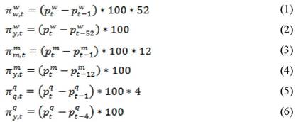Taking into account the seasonal effect on commodity prices, studies prefer monthly and quarterly price indices. This study deals with the monthly wholesale price index series. For the latter, there are two measures of the inflation rate: (i) the annual inflation rate (p_y) defined as the increase in the price index in the current month of the current year over the corresponding period of the previous year as shown in the equation 4 and (ii) the monthly inflation rate (p_m) defined as the increase in the price index between two consecutive months (the current month and the adjacent previous month), which is then multiplied by 1200 to arrive at the annualised inflation rate, as shown in the equation 3. Illustratively, the annual or the y-o-y inflation rate for the January 2008 would be estimated as the rate of increase in the price index for the month of January 2008 over the price index prevailing in January 2007. On the other hand, the monthly inflation rate for January 2008 would be estimated as the rate of increase in the price index for January 2008 over December 2007, which would then be multiplied by 12 to arrive at the annualised inflation rate. The monthly inflation rate shares an interesting relationship with the annual inflation rate, when the former is presented in terms of its moving average. Illustratively, for any point of time (or any month), let us take the moving average of the monthly inflation rate over 12 adjacent previous months:

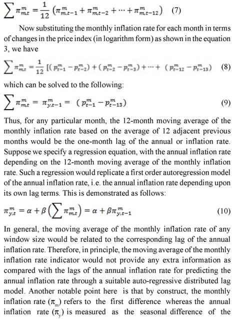logarithm transformed aggregate price index. Therefore, these two inflation rate indicators are likely to be different in terms of their stochastic properties. Now the pertinent question arises: Should pm be preferred to py? In what follows, we address various applied issues before taking up statistical exercises.

Section II

Some Applied Issues

From the perspective of policy objectives such as price stability, sustained growth and financial stability, authorities have to manage inflation expectations and inflation risks for various reasons. First, a low and stable price inflation environment is regarded as an essential condition for improving the growth and productive potential of the economy (Rangarajan,1997). Second, for risk pricing of financial products, the inflation expectation and the inflation risk premium form crucial components. According to the popular Fisher’s interest parity condition, the nominal return on a financial asset should equal to the sum of the real return and the expected inflation. The expectation of higher inflation and risks would be reflected in higher nominal interest rates (Berument,1999). Okun (1971) and Friedman (1977) argue that inflation is positively associated with inflation uncertainty, which is confirmed by a large body of empirical literature (Berument and Yuksel,2002, Ball, et.al.1992). As regards alternative inflation indicators, they may be associated with varying expectation and risk components, and thus, have implications for the volatility in financial markets. Moreover, a particular inflation rate indicator associated with greater expectation and risk than others may require frequent adjustment of policy instruments. Such a strategy may exacerbate uncertainties further with adverse consequences for investment and productive activities. According to Rangarajan (1997), volatility in prices creates uncertainty in decision making. Rising prices adversely affect savings while they make speculative investments more attractive. Second, the relationship of inflation rate with policy instruments and intermediate target variables such as monetary aggregates assumes critical importance. For authorities would be interested in knowing whether and to what extent the inflation condition is a monetary phenomenon. In this regard, deriving from Friedman’s view that ‘inflation is a monetary phenomenon’, price stability is understood in terms of monetary stability (Issing, 2000, Rangarajan, 1997). From the latter perspective, there are two important applied issues. One, whether alternative inflation rate indicators would show differential relationship with monetary variables? Second, the choice pertaining to a particular inflation rate indicator is two dimensional with respect to alternative inflation indicators and alternative monetary aggregates. Illustratively, inflation indicators may show differential correlation with narrow money than broad money aggregates. The narrow money comprising currency and demand deposit components reflects upon the transaction demand for money (Gauge, 1992). On the other hand, the broad money aggregate, apart from transaction demand, includes interest sensitive time deposits. Some researchers use the broad money aggregate to account for the wealth effect on consumption demand, apart from the transaction demand for money (Bredin and Cuthbertson, 2001). Third, the structural aspect of the inflation rate indicator, particularly, the inflation persistence, relating to the flexibility or the rigidity in the price setting behavior of producing sectors could also be another key issue for policy purposes. More persistent inflation may require more aggressive policy (Cecchetti and Debelle, 2004). Fuhrer and Moore (1995) show that when inflation is persistent, the output loss associated with disinflation is larger than when there is no persistence. Bordo and Haubrich (2004) find that the key factor in the yield curve’s ability to predict output growth is the persistence of inflation. They provide theoretical and empirical evidence that the yield curve has better predictive ability in regimes with high inflation persistence. According to Bilke and Stracca (2007), given the medium term perspective, authorities should put more emphasis on the more lasting movements and disregard the shocks that are likely to be soon reverted. Putting this idea into practice, this would imply excluding or giving less weight to the less persistent inflation processes. Blinder (1997) stated that it is important for policy to consider “what part of each monthly observation on inflation is durable and what part is fleeting”. Thus, the choice between alternative inflation rate indicators in terms of variance and persistence measures becomes extremely complex (Bilke and Stracca, 2007). A key lesson arising from the literature is that it is not the inflation variance and persistence, per se, which are important. Rather the implications of inflation persistence for economic fundamentals relating to financial markets, aggregate demand and growth are relevant. These considerations may entail that an inflation rate indicator which is smooth and less volatile be preferred to a more volatile indicator.

On the empirical plane, several stylised facts and time series properties of alternative inflation indicators could be exploited for policy analysis. First, for measuring inflation expectation and risks, a mute question here is how economic agents form expectations about future inflation condition. Before formal models such as adaptive expectation (Friedman, 1968) and rational expectation (Lucas, 1972) models were developed, economists believed in agents forming expectations based on the historical mean of the inflation rate observed over a sample period of medium-longer time horizon consistent with the maturity of benchmark financial instrument such as the ten-year treasury bond or the length of a typical business cycle. In recent years, economists use a variety of time series models to measure time varying inflation expectations in line with the alternative expectation models. Illustratively, the auto regressive integrated moving average (ARIMA) model is used widely to measure adaptive expectation component of the inflation rate. Second, as regards the measure of inflation risk, a commonly adopted measure of inflation risk is the unconditional standard deviation of inflation rate over a sample period preferably over medium-longer horizon. Since economic agents engage in dynamic financial risk pricing in a modern financial environment, the conditional or time varying inflation risks based on generalised auto regressive conditional heteroscedacity (GARCH) models for the inflation rate are becoming popular. Third, for gauging the inflation persistence, empirical studies have adopted various approaches such as lagged correlation of inflation, the correlation of inflation with the growth rate of monetary variables, Box-Jenkin’s ARIMA model and Granger’s spectral density analysis.

The following section dwells on empirical exercises based on the above time series models.

Section III

Empirical Evidence

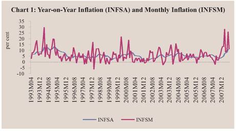
Chart 1 shows the two measures of inflation rate i.e., annual inflation rate (INFSA) and the monthly inflation rate (INFSM), derived from the seasonal adjusted (using X12 method) wholesale price index over the sample April 1993 to July 2008. It is evident that the annual inflation rate is smoother than the monthly inflation rate series. The latter is more or less symmetrically distributed around the former. This is evident from the monthly inflation rate being lower than the annual inflation rate for 97 months or 53 per cent of the sample period comprising 184 months data. At the same time, the monthly inflation rate was above the annual inflation rate for 87 months or 47 per cent of the sample. The monthly inflation rate is highly volatile; at times, it could be higher than 20-30 per cent on annualised basis and such high rates generally being followed by low or negative values. The monthly inflation rate was negative for 18 months during the sample period; the lowest was at -6.4 per cent in February 1998. But the annual inflation rate was never negative during the same period. The monthly inflation rate was above 10 per cent for 44 months out of 184 months. On the other hand, the annual inflation rate was above 10 per cent for 17 months out of 184 months. The monthly inflation rate was above 6 per cent for 80 months whereas the annual inflation rate was above 6 per cent for 70 months. However, the two inflation indicators had a contemporaneous correlation at 0.44, implying that they did not move perfectly in tandem with each other.

III.1 Stylised Facts

III.2 Inflation Expectation and Persistence

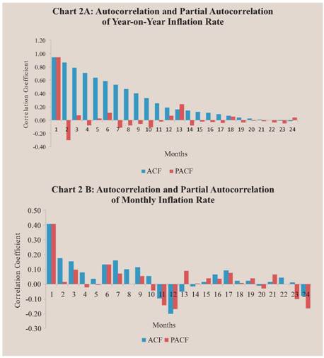
The persistence of an economic indicator, prima facie, is gauged from its auto-correlation (ACF) and partial auto correlation (PACF) functions, which form a part of identification of a suitable ARIMA model. Chart 2 shows the autocorrelation of two inflation rate indicators over 24 months. The auto correlation of annual inflation indicator is statistically significant up to 13 lags, as it remains away from 2 asymptotic standard errors band. The partial auto correlation of annual inflation rate could be statistically significant only for two lags. The behavior of ACF and PACF of the annual inflation indicator suggests that the variable could be modeled with a first order ARIMA model. On the other hand, for the monthly inflation rate, the auto-correlation is significant up to 3-lags while the partial auto correlation is significant for 1-lag (Chart 2). Moreover, the lagged correlations of the monthly inflation rate are significantly low as compared with the lagged correlations of the annual inflation rate. Thus, the correlogram of annual inflation and monthly inflation rates suggests that the former could be more persistent than the latter. However, such inference about the nature of persistence in two inflation indicators could be erroneous without consideration of stochastic properties of the variables (Cochrane, 1988).

Is the Inflation Rate a Stationary Process?

Nelson and Plosser (1981) showed that the behavior of an economic variable in response to various shocks depend critically on its stochastic nature, which is reflected in the random walk component and analysed through the unit root test. They showed that unanticipated shocks do not affect the permanent or long-run trend component of a stationary economic variable, and thus, such a variable would be least persistent. According to Cochrane (1988), the long-range forecast for a stationary series tends to converge with its historical mean. Of particular interest to the inflation rate, research shows that the measures of expectation, persistence and permanent components cannot be analysed without first-hand knowledge whether the inflation rate is a stationary series. Table 3 presents result of the unit root for the two inflation indicators under investigation. It is evident from various unit root tests that the monthly inflation rate, which is the first difference of log-transformed price index, is a stationary process, a finding most common to the empirical literature. On the other hand, various unit root tests do not provide a unique answer to whether the annual inflation rate is a stationary process. The Kwzatkowkz, Phillips, Schmidt and Shin (KPSS) and Eliot, Rothenberg and Stock - Dicxey - Fuller generalised least square (GLS) tests suggest that annual inflation rate is a stationary process while the conventional Augmented Dicxey - Fuller (ADF ) and Phillips-Perron (PP) tests provide the contrasting evidence. An interesting observation here is that the choice of the sample period could play an important role for the existence of unit root in the annual inflation rate. Illustratively, the ADF test rejects the annual inflation rate as a stationary variable for the sample April 1993 to July 2008. However, the same test could prove the annual inflation rate as a stationary process for the sample period April 1995 to July 2008 (up to July), excluding the episodes of high inflation rates during April 1993-March 1995.

At a formal level, inflation persistence can be measured in various ways. First, as shown by Levin and Pinger (2004) and Cecchetti and Debelle (2005), the measure of persistence (s) in the inflation rate can be estimated from the auto-regressive distributed lag model such as the following:

Second, Campbell and Mankiew (1988) suggested that the popular ARMA (p, q) model can also be used to estimate the persistence parameter (s). Illustratively, from the first order ARMA (1, 1) model, the persistence measure can be estimated as higher the autoregressive coefficient, higher the persistence and higher the moving average parameter, lower the persistence. Table 4 presents the estimated first order ARMA (1, 1) model for two inflation indicators. The coefficients of AR and MA terms suggest that the annual inflation is more persistent than the monthly inflation rate. The intercept term in the ARMA model suggests more or less similar mean for both the inflation rates. However, it is evident from the coefficient of determination R2 that the ARMA (1, 1) model fits well with the annual inflation rate but not the monthly inflation rate. Also, in terms of inflation forecasts out of sample for 7 months during January-July 2008, the ARMA model performs better for the annual inflation rate than the monthly inflation rate, which is evident from various forecast error statistics reported in the Table 4. Thus, inflation expectation can be gauged better with the annual inflation rate than the monthly inflation rate. Tables 5a and 5b present the results of the ARDL model for analysing persistence in the annual and monthly inflation rates respectively. The coefficient of the first order autoregressive component of the inflation rate, which reflects on persistence, for the annual inflation rate is twice that of the monthly inflation rate. The Wald test suggested that null hypothesis of unity persistence coefficient for the annual inflation rate could be rejected at five per cent level of significance. Interestingly, both the equations in Table 5a and 5b suggest similar long-run expected inflation for the annual and the monthly inflation rates at 5.6 per cent.

Power Spectrum of Inflation Rates

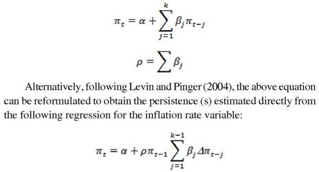
Following Granger’s (1966) work on spectral density function of economic variables, several empirical studies have used this methodology to measure persistence (Levy and Dezhbakhsh, 2003) According to Granger (1966), “the long -term fluctuations in economic variables, if decomposed into frequency components, are such that the amplitude of the components decreases smoothly with decreasing period”Cochrane (1988) suggested that the persistence of a stationary series can be measured by the power spectrum at zero frequency. 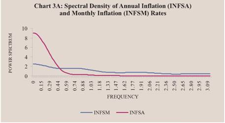In other words, if the spectral density function for an inflation rate indicator were to follow a downward sloping curve, then the behavior of inflation rate would be driven by long-term economic fundamentals. In such a situation, inflation would be less volatile and highly persistent. Otherwise, for an upward sloping spectral density curve, the inflation rate would be driven by various short-term factors and it would be highly volatile and less persistent, with little role for economic fundamentals. Chart 3A shows the spectral density function of annual and monthly inflation rates, based on Bartlet’s window. The SDF of both annual and monthly inflation rates falls through low to high frequencies or long to shorter time horizons. However, at zero frequency, the estimated power spectrum of the annual inflation rate is three times larger than that of the monthly inflation rate. For business cycle and shorter period frequencies (above >=0.8), the estimate of power spectra for the monthly inflation is much larger than the annual inflation rate. Thus, it can be inferred that the permanent or the long-term component could be larger for the annual inflation rate than the monthly inflation rate. Interestingly, if the annual inflation rate were to be considered a stationary process in the first difference form (DINFSA), then its spectral density function would show the power spectrum at zero frequency lower than the monthly inflation rate (Chart 3B).

III.3 Inflation Volatility

III.4 Inflation and Money Growth Relationship

Table 7 presents the contemporaneous correlation of inflation rate (INFSA) with growth rates of reserve money (GRMSA), narrow money (GM1SA) and broad money (GM3SA) aggregates in the hierarchy of liquidity. There are a couple of interesting insights emerging from the correlation analysis. First, it is evident that the annualised inflation rate has significant correlation with the annual growth rates of reserve money, narrow money and broad money aggregates. However, the monthly inflation rate does not have significant contemporaneous correlation with the monthly growth rates of monetary aggregates.

Recognising the transmission lags, Table 8 presents the correlation of inflation rate with lags in the growth rate of monetary aggregates. It is evident that the correlation of annual inflation rate with lags of growth rates of reserve money and narrow money are significant up to 13 months. The correlation of annual inflation with the lags of the growth rate of broad money is significant up to eight months and in terms of magnitude, it is weaker than the narrow money aggregate. On the other hand, the monthly inflation rate does not show significant correlation with lags of the growth rate of narrow and broad monetary aggregates.

Beyond correlation analysis, it is useful to study the formal Granger causality between inflation rate and money growth indicators (Table 9). The causal relationship between inflation rate and money growth indicators is shown for various lags in line with various lag selection criteria. Illustratively, in the two-variable VAR framework, the Swarzt-Bayes and the Hannan-Quinn criteria suggested 1-2 lags. On the other hand, the final prediction error, Akaike information and modified likelihood ratio criteria suggested for higher order lags up to 12 or 13 months. First, for lower order lag model such as 1-month lag, the annual inflation significantly Granger causes narrow money growth rate at 5 per cent level of significance and the narrow money growth could Granger cause annual inflation rate vice versa but at a higher 10 per cent level of significance. For the same lag order, there is no causal relationship between annual inflation and reserve money growth rates. The broad money growth rate Granger causes the annual inflation rate albeit, at higher 10 per cent level of significance, but the annual inflation rate does not Granger cause the broad money growth rate. On the other hand, the monthly inflation does not have causal relation with monthly growth of reserve money and narrow money indicators. Only the monthly growth rate of broad money could Granger cause the monthly inflation rate but at higher 10 per cent level of significance. As we increase the lag length to 2 to 3 months, there is a significant change in the causal nexus between inflation and narrow money growth indicator. For 2-3 lags, the annual growth rate of narrow money significantly Granger causes the annual inflation rate, not vice versa, which was observed in the case of 1-month lag case. However, in terms of monthly variation, both narrow money growth and inflation rate Granger cause each other. On the other hand, the causal relationship between the broad money growth and the inflation rate remains more or less similar for lower order lags of 1-3 months. Reserve money growth does not cause inflation for similar lower order lags. Second, for higher order lags such as 12 to 13-months, annual narrow money growth and inflation rates show simultaneous granger causal relationship. In terms of monthly variation, however, it is the narrow money growth which causes the inflation rate. On the other hand, both monthly and annual variations in broad money Granger cause the inflation rate and the latter does not cause the former.

Though the causal analysis shown in the Table 9 provides some useful information, it cannot substantiate the strength of the relationship between inflation and monetary aggregates, especially with respect to the models involving monthly and annual inflation rates. In this regard, we engage in two more statistical analyses as follows. First, we examine the coefficient of determination of inflation and money growth equations arising from the VAR models underlying the Granger causal analysis (Table 10). A key finding in terms of coefficient of determination is that the VAR model involving annual inflation and money growth indicators significantly outweighs the similar model involving monthly inflation and money growth indicators. Second, as shown in Reddy (1998), we undertake non-nested regression analysis to know whether it is the narrow money or the broad money growth indicators which is more informative for explaining the monthly or annual inflation rates. The results of nested regression analysis are presented in Table 11. Two crucial findings emerge. One, the monthly growth of broad money could be preferred to the monthly growth of narrow money for predicting monthly inflation rate. Two, the annual growth rate of narrow money could be preferred to the annual growth rate of broad money for predicting the annual inflation rate. Thus, it can be inferred that annual inflation has better correlation with annual growth of monetary variable, especially, the narrow money aggregate, which reflects upon the transaction balance relation of money with inflation.

III.5 Inflation and Growth Causal Nexus

How do alternative measures of the inflation rate affect economic growth? In this regard, Tables 12(a) and (b) present the results of Granger causality between inflation rate and the growth of industrial production (seasonally adjusted) based on two-variable VAR model. It is evident that for 1-lag model, the annual inflation rate Granger causes the annual and the monthly growth rates of industrial production but not vice versa (Table 12a). For 12-month lag model, the annual inflation rate Granger causes the annual industrial production growth but not vice versa (Table 12b). However, there exists no Granger causal relationship between the monthly inflation rate and the monthly growth of industrial production for both 1-lag and 12-lag models. Such empirical findings were also evident for various other lags.

III.6 Inflation and Financial Markets

Table 14 presents the correlation of annual and monthly inflation rates with annual and monthly variation in equity prices respectively. The lags in annual inflation rate do not have significant correlation with the annual variation in equity prices. On the contrary, the correlation of lags in annual variation in equity prices with the annual inflation rate becomes significant after 3 months and this continues up to about a year. Thus, the annual inflation rate and the annual variation in equity prices share Granger causal relationship. However, the monthly inflation rate and the monthly variation in asset prices do not have significant correlation and Granger causal relationship.

Section IV
Conclusion

The inflation rate indicator is not directly observed; it is derived as the percentage increase in the observed aggregate price indices between two time periods. Generally, the inflation rate defined as the rate of increase in the aggregate price index between two discrete time period can be derived statistically for various frequencies such as weekly, monthly, quarterly and annual basis. However, in practice, central banks measure the inflation rate as the year-on-year percentage increase in the price index. This study discussed various applied issues associated with two alternative measures of the inflation rate indicator such as the monthly (month-over-month) and the annual (year-on-year) changes in the wholesale price index in India. Empirical results provide a couple of insights pertaining to these inflation rates and their association with monetary aggregates, output, interest rate, and equity prices. First, the sample means of these two inflation rates could not be statistically different from each other. However, the volatility of the monthly inflation rate could be significantly different from the volatility of the annual inflation rate. Second, the annual inflation rate could be more persistent than the monthly inflation rate, attributable to the long-term component. From the perspective of policy objectives such as price stability, a smoothed and less volatile annual inflation rate would be more useful than the highly volatile monthly inflation rate. Third, the ARMA model, which is often used for gauging inflation expectation and persistence, could fit the annual inflation rate better than the monthly inflation rate. A similar finding also emerged for the GARCH model, which is used for analysing the interaction between inflation expectation and volatility components. Fourth, the correlation of the annual inflation rate with the annual growth rate of monetary aggregate was stronger than the correlation of monthly inflation rate with monthly growth rates of monetary aggregates. The order of liquidity effect, as reflected in the narrow and broad money aggregates, had differential causal effect on the inflation rate. Narrow money growth had stronger correlation with inflation, in line with the standard transaction demand for money hypothesis. Fifth, the annual inflation rate showed statistically significant Granger causal relation with the annual growth rate of industrial production. However, such causal relationship did not exist between the monthly inflation and output growth rates. Overall, these findings support that the standard year-on-year inflation rate could be more useful than the monthly inflation rate for policy analysis.

¹ Janak Raj is Adviser and Sarat Dhal is Assistant Adviser in the Department of Economic Analysis and Policy, Reserve Bank of India, Mumbai. The views expressed in the paper are of the authors’ only and the not the organisation to which the authors belong.

Notes

1 Dr. Bimal Jalan, the former Reserve Bank Governor, pointed out that the core inflation does not reflect the Indian scenario, as it accounts for just 30 per cent of the actual inflation rate, excluding rising prices of food and petroleum products: http://inhome.rediff.com/money/2003/oct/03jaswant.htm?zcc=rl

2 See the press interview of Dr. Y.V. Reddy, Governor, Reserve Bank of India in the Hindus Business Line, April 7, 2007:http://www.thehindubusinessline.com/2007/04/27/stories/2007042700480800.htm

3 See “IMF paper moots new method, puts inflation at 4.7 pc” Hindustan times May 21 2008 also in AsiaViews, Edition: 17/V/Mayl/2008, and http:// www.indianexpress.com/story/22926.html.

4 Michael Burda and Charles Wyplosz(1997), Macroeconomics: A European text, 2nd ed., p. 579 (Glossary). Olivier Blanchard (2000), Macroeconomics, 2nd ed., Glossary. Robert Barro (1993), Macroeconomics, 4th ed., Glossary. Andrew Abel and Ben Bernanke (1995), Macroeconomics, 2nd ed., Glossary. Ludwig von Mises, The Theory of Money and Credit, Jesus Huerta de Soto, Money, Bank Credit, and Economic Cycles.

5 www.economist.com

6 http://www.bankofengland.co.uk/education/targettwopointzero/inflation/whatsInflation.htm

7 http://www.cbc.ca/news/background/economy/inflation.html

8 See Chapter IV in the “Report of the Working Group on Money Supply Analytics and Methodology of Compilation” Chairman Dr Y V Reddy Reserve Bank of India 1998

References:

Abel, A. and Ben Bernanke (1995), Macroeconomics, 2nd ed., Glossary.

Alchian, A.A. and Klein, B. (1973), “On a Correct Measure of Inflation”, Journal of Money, Credit and Banking, Vol. 5,No.1, pp. 173-91.

Andrews, D.W.K. and Chen, H.Y.(1994), “Approximately Median-unbiased Estimation of Autoregressive models”, Journal of Business and Economic Statistics 12 (2), 187–204.

Barro, R.J. (1991) “Economic Growth in a Cross Section of Countries”, Quarterly Journal of Economics, vol. 106, May pp-407-443.

Ball, L. (1992), “Why Does High Inflation Raise Inflation Uncertainty?” Journal of Monetary Economics, 29, 1992: 371-88.

Ball, L. and Cecchetti, S.G. (1990), “Inflation and Uncertainty at Short and Long Horizons” Brooking Papers on Economic Activity, No.1.

Ball, L.(1994), “Credible Disinflation with Staggered Price-setting”, American Economic Review, 84(1), pp 282– 89.

Berument, H.(1999),“The Impact of Inflation Uncertainty on Interest Rates in the UK” Scottish Journal of Political Economy, May 1999: 207-18.

Berument, H. and Yuksel, M. (2003), “Temporal Ordering of Inflation and Inflation Uncertainty Evidence from the United Kingdom”, Bilkent University Turkey.

Bhattacharya, R., Patnaik, Illa, and Shah, A. (2008), “Early Warnings of Inflation in India”, National Institute of Public Finance and Policy, New Delhi.

Bilke L and Livio Stracca (2000), “A Persistence-weighted Measure of Core Inflation in the Euro area, Economic Modelling 24 (2007) 1032–1047

Blinder, A. (1997), “Commentary”, Review. Federal Reserve Bank of Saint Louis. May–June.

Borio, C., Kennedy V., and Prowesh, S.D.(1994), “Exploring Aggregate Price Fluctuations Across Countries Measurement, Determinants and Monetary Policy Implications”, BIS Working Paper, No.40, BIS, Basle.

Bredin, D. and Cuthbertson, K. (2001), “Liquidity Effects and Precautionary Saving in the Czech Republic”, Central Bank of Ireland Technical Paper 4/ RT/01.

Bryan, M.F., Cecchetti, S.G. and Sullivan, R.O.(2002), “Asset Prices in the Measurement of Inflation”, NBER Working Paper No.8700, January.

Bryan, M.F. and Cecchetti, S.G. (1993), “Measuring Core Inflation”, Economic Review. 29, Federal Reserve Bank of the US.

Bryan, M.F. and Cecchetti, S.G. (1994), “Measuring Core Inflation”, in Monetary Policy, ed. N. Gregory Mankiw, Chicago: University of Chicago Press.

Bryan, M. F. and Christopher, P. (1991), “Median Price Changes: an Alternative Approach to Measuring Current Monetary Inflation”, Economic Commentary. Federal Reserve Bank of Cleveland, December.

Burda, M. and Wyplosz, C. (1997), “Macroeconomics: A European text”, 2nd ed., p. 579 (Glossary).

Cecchetti, S.G. (1995), “Distinguishing Theories of Monetary Transmission Mechanism”, Federal Reserve Bank of St Louis Review, 77(3).

Cecchetti, S., G., Lipsky, H. J. and Wadhwani, S., (2000), “Asset Prices and Central Bank Policy”, Report prepared for the Conference “Central Banks and Asset Prices”, organised by the International Center for Monetary and Banking Studies and CEPR in Geneva on May 5.

Cecchetti, S.G. and Debelle, G. (2003), “Has the Inflation Process Changed?” Third BIS Annual Conference, Understanding Low Inflation and Deflation, Brunnen, Switzerland, June 2004.

Chetty,V. K. (1969),“On Measuring the Nearness of Near-Moneys”, The American Economic Review, Vol. 59, No. 3.

Cutler, J. (2001), “A New Measure of Core Inflation in the UK”, MPC Unit Discussion Paper, vol. 3, Bank of England.

Clark , T.E. (1997), “Cross-country Evidence on Long-run Growth and Inflation”, Economic Enquiry, vol.35., January.

Sarel, M (1996), “Non-linear Effects of Inflation on Economic Growth”, IMF Staff Papers, vol 43. No. 1.

Cutler, J., 2001. A new measure of core inflation in the UK. MPC Unit Discussion Paper, vol. 3.

Dias, D. and Marques, R.C. (2005), “Using Mean Reversion as a Measure of Persistence”, European Central Bank Working Paper Series, vol. 450.

Eckstein, O. (1981), “Core Inflation”. Englewood Cliffs: Prentice-Hall.

Fisher, I. (1906), “Nature of Capital and Income”, New York: Macmillan.

Friedman, Milton (1968), “The Role of Monetary Policy," American Economic Review, 58,

Friedman, Milton (1977),“Nobel Lecture Inflation and Unemployment,” Journal of Political Economy, 85.

Fuhrer, J and G Moore (1995), “Inflation Persistence”, Quarterly Journal of Economics, vol. 110.

Gauger, J. (1992), “Portfolio Redistribution Impacts within the Narrow Monetary Aggregate Journal of Money, Credit and Banking, Vol. 24, No. 2. (May, 1992), pp. 239-257.

Goodhart, C., What Weight Should be Given to Asset Prices in the Measurement of Inflation?

Goodhart, C. and Hofmann, B. (2000), “Do Asset Prices help to Predict Consumer Price Inflation?” The Manchester School Supplement, 68.

Goodhart, C. and Hofmann, B. (2001), “Asset Prices and the Conduct of Monetary Policy”, paper presented at the Swedish Riksbank Conference on Monetary Policy, June 2000.

Granger, C.W.J.(1969), “Investigating Causal Relations by Econometric Models and Cross-Spectral Models, Econometrica, 37.
Issing, O. (2003), “Monetary and Financial Stability - is there a Trade-off?” BIS Review, No.16.

Kannan, R. and Joshi, H. (1998), “Growth-Inflation Trade-off: Empirical Estimation of Threshold Rate of Inflation for India”, Economic and Political Weekly, October.

Lebow, D. E. and Rudd, J. B. “Measurement Error in the Consumer Price Index Where Do We Stand?” Journal of Economic Literature 41.

Lucas, R. (1972), “Expectations and the Neutrality of Money", Journal of Economic Theory.

Ludwig von Mises, “The Theory of Money and Credit”, Jesus Huerta de Soto, Money, Bank Credit, and Economic Cycles.

Okun, Arthur (1971), “T he Mirage of Steady Inflation,” Brooking Papers on Economic Activity, 2, 1971.

Robalo, Marques C. (2004),"Inflation Persistence: Facts or Artifacts", ECB Working Paper No. 371, June 2004;

Mohanty,D., Rath, D.P. and Ramaiah, M. (2000), “Measuring Core Inflation for India” Economic and Political Weekly, Vol. 35 No.5.

Raipuria, K. (2003), “Dynamics of Inflation in Services”, Economic and Political Weekly, Vol. 38 No. 26.

Rangarajan, C. (1997), “The Role of Monetary Policy”, Ninth V.T. Krishnamachari Memorial Lecture, BS_SpeechesView.aspx?Id=252

Reddy, Y.V. (1998), “Report of the Working Group on Money Supply: Analytics and Methodology of Compilation”, Reserve Bank of India, Mumbai.

Rosen, S. (1974), “Hedonic Prices and Implicit Markets Product Differentiation in Pure Competition”, Journal of Political Economy, Vol. 82, No. 1.

Roubini, N. (2006), “Why central banks should burst bubbles”, Working Paper, New York University, Stern School of Business.

Samanta, G. P. (1999), “Core Inflation in India”, Reserve Bank of India Occasional Papers, Vol 20, No 1.

Samanta, G P and Mitra, S. (1998), “Recent Divergence between Wholesale and Consumer Prices in India–A Statistical Exploration”, Reserve Bank of India Occasional Papers, Vol 19, No 4, December, pp 329-44.

Samuelson, P. (1961), “The Evaluation of Social income, Capital formation and Wealth”, in (F Lutz and D Hague eds.), The Theory of Capital, London: Macmillan.

Saxton, J. (2003), “Monetary Policy and Asset Prices”, A Joint Economic Committee Study, United States Congress.

Shibuya, H. (1992), “Dynamic Equilibrium Price Index, Asset Price and Inflation”, Bank of Japan Monetary and Economic Studies, Institute for Monetary and Economic Studies (IMES), Bank of Japan, Vol. 10. No.1.

Shiratsuka, S. (1999), “Asset Price Fluctuation and Price Indices”, IMES Discussion Paper, No 99-E-21, Bank of Japan.

Shiratsuka, S. (1997), “Inflation Measures for Monetary Policy: Measuring the Underlying Inflation Trend and Its Implication for Monetary Policy Implementation”, Monetary and Economic Studies, 15(2), Institute for Monetary and Economic Studies, Bank of Japan, pp 1-26.

——— (1999a) “Measurement Errors in the Japanese Consumer Price Index”, Monetary and Economic Studies, Vol.17, no.3, Institute for Monetary and Economic Studies, Bank of Japan.

——— (1999) “Asset Price Fluctuation and Price Indices”, Monetary and Economic Studies, 17(3), Institute for Monetary and Economic Studies, Bank of Japan, pp 103-28.

——— (1995), “Effects of quality changes on the price index: A Hedonic approach to the estimation of a quality-adjusted price index for personal computers in Japan”, Bank of Japan Monetary and Economic Studies, Institute for Monetary and Economic Studies, Vol. 13, No. 1.

Srinivasan, T. N. (2008), “Price Indices and Inflation Rates”, Economic and Political Weekly, Vol. 43 No. 26.

Vasudevan, A. (1998), “Analytical Issues in Monetary policy in transition”, Reserve Bank of India Bulletin, January 1998.

Vasudevan, A., B. K. Bhoi, and Dhal, S.C. (1999), “ Inflation and Optimal Growth” in Fifty Years of Development Economics in India, (eds. A Vasudevan, D. M. Nachane, A. Karnik) Himalay Publsihing  House, New Delhi.