Harendra Kumar Behera and Rajiv Ranjan*

This paper empirically examines neoclassical prediction of financial globalization impact on growth in emerging market economies. Unlike other studies to use five year average to capture business cycles, the paper uses annual data for 27 countries for the period 1980 through 2007 to capture time series properties of the data. Using panel cointegration tests, the study found a long-run relationship between per capita income and financial globalization. The long-run coefficient of financial globalization impact on per capita GDP was estimated using panel FOLS and DOLS and found to be positive. The results remained unchanged controlling for trade openness.

JEL Classification : F36, C33, C22

Keywords : Financial Globalization, panel FMOLS, panel DOLS, panel cointegration.

Introduction

Finance does matter for economic growth and therefore opening up of the economy to receive financial flows by a resource scarce country. Capital account liberalisation has a number of benefits in terms of development of institutions, filling-up the resource gap and ultimately growth of the economy. On the other hand, the more financially integrated economy requires insurance to protect against the risks stemming from such financial openness. Many researchers have also found that opening up of a country is associated with likelihood of happening a crisis. Further, the way the current global financial crisis turned out has brought to the forefront the important role that finance play, reminding the costs and benefits associated with financial globalization.

The phenomenon of large capital flows led by cross border trade of financial assets is not new to the emerging market economies (EMEs). The early wave of financial globalization traced back to a century old where the exchange rate system was fixed¹. Integration was high in 1870–1914, declined sharply through the Great Depression and World War II, and subsequently recovered – gradually during the following two decades, and more rapidly beginning in the 1970s (Obstfeld and Taylor, 2004). The beginning of the twenty first century witnessed the level of integration that had experienced during 1870–1914. The new phase of financial globalization began with improvements in information technology and the removal of barriers to the free flow of capital across countries in the mid-1980s.

The recent episodes of capital flows to the EMEs have been debated because of their abrupt movement and resultant impact on asset prices and exchange rates, and ultimately the impact transmitted to the real sector of the economy. It is also argued by critics of financial globalization that international capital mobility may increase the probability of financial crisis (Reinhart and Reinhart, 2008). Financial globalization carries some degree of risk as evidenced from financial crisis in Asia and Russia in 1997-98, Brazil in 1999, Ecuador in 2000, Turkey and Argentina in 2001, and Uruguay in 2002. However, as Schmukler (2004) argued, crises were not just due to financial globalization. According to him, evidence suggests that crises are complex and have been a recurrent feature of financial markets for a long time, both in periods of economic integration and disintegration. The root cause of almost all the crisis could be attributed to the problem of information asymmetries rather than financial globalization itself. The net benefit of financial openness is large if it is managed well. The management is important because financial globalization is likely to deepen over time, led by its potential benefits. While the theoretical benefits of financial integration essentially presume a perfect market condition, the real world financial system operates through imperfect environment. It is, therefore, more important to know the costs and benefits associated with financial globalization. The large capital inflows (outflows) make the job of the policy makers of EMEs complex as they could deter also the expected benefits of financial globalization. Looking at the above issues, the time has come to examine whether capital account openness is beneficial for a country.

During the last few years, the EMEs experienced both large capital inflows and capital outflows². Concomitantly, the emerging countries have also passed through phases of higher growth trajectory along with large reserve accumulation. The large reserve accumulations have helped these countries to sustain the adverse impact of the global crisis without having much damage. High growth in the EMEs also helped in taking strong policy decisions to further develop these economies. Besides, the EMEs, who had experienced larger capital flows in recent decades, were remained resilient during the crisis period. Although there are signs of positive effect of financial globalization on growth, empirical studies hard to find any such impacts. With this background, the paper is attempting to empirically examine the relationship between economic growth and financial globalization in EMEs. The following section provides the theoretical and empirical issues associated with the financial globalization and growth nexus. Section III of the paper traces the episodes of economic growth and the nature of capital flows to EMEs. A discussion about sources of data, different variables and methodology used in the study is presented in Section IV. Section V examines the empirical relationship between capital account openness and growth in EMEs and concluding observations are list out in final Section.

Section II
Theoretical and Empirical Issues in Financial Globalization

It is widely accepted in the theory that capital account liberalization has many positive effects, viz. capital account liberalization increases economic growth, encourages financial development and portfolio diversificaion. The neoclassical growth model suggests about a positive impact of capital account liberalization on growth through a more efficient international allocation of resources. Resources flow from capital-abundant developed countries, where the return to capital is low, to capital-scarce developing countries where the return to capital is high³. The flow of resources into the developing countries reduces their cost of capital, triggering a temporary increase in investment and growth that permanently raises their standard of living (Henry, 2007). Financial globalization can play an important role in encouraging development of institutions so that financial markets can effectively perform the crucial function of getting capital to its most productive uses which is key to generating growth and reducing poverty (Mishkin, 2005). The other view provided by some economists that removing one distortion – restrictions to capital movement – in the presence of other distortions that often exist in emerging markets- may not necessarily enhance welfare (e.g. Newbery and Stiglitz, 1989; Stiglitz, 2008). The later view gained relevance after occurrence of a couple of crises in the 1990s and the recent global financial crisis. Whereas the theory stands strong on positive growth impact of capital account liberalization, a number of cross-country literature on financial globalization hardly found any such positive impact on growth.

Though there is broad consensus about the relationship between financial globalization and economic growth, conflicts do exist while it is examined in practice. Financial globalization or capital flows and economic growth nexus has spurred volumes of empirical studies on both cross country and individual country cases. One of the earliest well known works by Rodrik (1998) shows that there is no evidence of positive impact of capital account liberalization on growth. On the contrary, another much cited paper by Quinn (1997) using IMF’s Annual Report on Exchange Rate Arrangements to measure financial liberalization finds a positive relationship between the decline in restrictions to the capital account and growth. Thereafter many works based on Quinn’s measure of financial globalization or with some refinement to that measure find mixed results while examining the relationship with growth.

The empirical literature on financial globalization and growth linkage is still to be corroborated as a little robust evidence exists in the context of the growth benefits of capital account liberalization. However, a number of recent papers in the finance literature report that equity market liberalizations do significantly boost growth. Thus, the empirical literature on overall impact of financial globalization is at best ambiguous. Surveying a large number of studies, Eichengreen (2001) concluded that the findings in literature are ambiguous on the evidence that liberalization has any impact on growth. In a comprehensive survey of research on financial globalization, Kose, et al (2006) reported that the majority of these studies, however, tend to find no effect or at best a mixed effect for developing countries. The apparent absence of robust evidence of a link between financial globalization and economic growth may not be surprising, in light of the well-known difficulties involved in finding robust determinants of economic growth in cross country or panel regressions. Critically examining the empirical studies on financial globalization, Henry (2007) strongly pointed out that the failure of existing studies to detect a positive impact of financial globalization on growth as the studies look for permanent growth effects whereas in the neoclassical growth model permanent decreases in the cost of capital and hence increase in the ratio of investment to GDP only have a temporary effect on growth. The model makes no predictions about the correlation between capital account openness and long-run growth rates across countries, and certainly does not suggest the causal link needed to justify cross-sectional regressions. What the neoclassical model predicts is that liberalizing the capital account of a capitalpoor country will temporarily increase the growth rate of its GDP per capita and thus, permanently increase the level of GDP per capita.

Neoclassical growth models with well defined steady states expect a long-run relationship between the levels of output and investment. Further, the model including only the growth rate of GDP excludes the neoclassical growth models by assumption, instead of including these models in conjunction with endogenous growth models (Hansen and Rand, 2005). Therefore, we have considered level of per capita GDP and financial globalization (net capital flows to GDP ratio) in our empirical model instead of GDP growth. As reported by Behera (2008), this relationship is parallel with the relationship between GDP (or GDP per capita) and domestic investment⁴. It may also be possible that economies do not converge to steady states (e.g.AK-type models of growth) or foreign investment has an impact on total productivity so that a rise in the financial globalization leads to permanent movements in the steady states.

Since earlier studies considered growth rates of GDP or per capita GDP to study the relationship between financial globalization and economic growth failed to examine the timeseries property of the data in levels. Using GDP per capita instead of growth rate of the same, we have advantage of studying both the long-run and short-run relationship along with cross-sectional impact in our study. Along with large cross-sections, long-timeseries data have the benefit of examining the dynamic link between financial openness and economic growth by using recently developed panel techniques, viz. panel cointegration tests, and fully Modified OLS (FMOLS) and dynamic OLS (DOLS) techniques.

Section III
Stylized Facts of Capital Flows and Growth in EMEs

With the increase in total net capital inflows to the EMEs, the net private capital flows have become dominant during the 1990s and 2000s (Figure 1)⁵. Direct investment component of private capital inflows continued to remain large and stable over the years despite the crises in different phases reflecting the long-term interest of the investors in EMEs. In the 1970s and 1980s, private capital flows to EMEs were concentrated in Latin America. During the last one and half decades, the emerging Asia and emerging Europe became important destinations for private financial flows.

In the early 1980s, with sharp decline in commodity prices, international interest rates rose to unprecedented levels, and economic activity in industrialized countries slumped. This pushed many EMEs into financial difficulties. Starting with Mexico in August 1982, a number of Latin American nations announced moratoriums on their sovereign obligations. As a result of the above, the net private capital inflows to EMEs turned negative in 1984. However, introduction of several lending plans by the International Monetary Fund (IMF) and development banks, led to increase both official and bank loan flows to EMEs during the 1980s. The Brady Plan of 1989 allowed countries experiencing debt crises to restructure their debt by converting existing bank loans into collateralised bonds at a significant discount or at below market interest rates. Financial flows to EMEs resumed quickly following the Brady exchanges in the early 1990s. A notable feature of this period was the surge in the flow of capital to EMEs in Asia, notwithstanding the high domestic savings rates (Perrault, 2002).

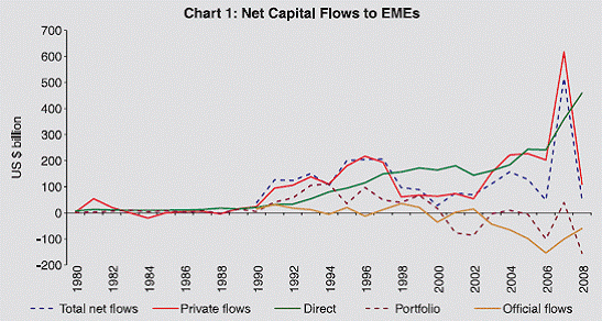As against official capital dominated regime, the 1990s saw a shift to non-debt-creating forms of capital inflows, and direct investment became the principal source of new capital available to EMEs. Importantly, direct investment has remained strong even in the aftermath of the crises in EMEs during 1997-1998. In contrast, the EMEs started exporting other types of capital flows, particularly interbank lending and portfolio flows.

During the 2000s, the emerging Asia and emerging Europe are the dominants in receiving the largest amount of private capital flows (Table 1). Furthermore, among the emerging countries, some countries tend to receive large amounts of inflows while other countries receive little foreign capital. As a consequence, the share of flows dedicated to relatively low- and middle-income emerging countries has decreased over time. This pattern is important to be noted because if countries benefit from foreign capital, only a small group of countries are the ones benefiting the most. The unequal distribution of capital flows is consistent with the fact that the income among developing countries is diverging although the causality is difficult to determine (Schmukler, 2004).

Another notable feature of emerging market economies is that the current account balance became positive since 2000 as against net deficits during the 1980s and 1990s (Figure 2). Furthermore, net private capital flows remained buoyant during mid-1990s and 2000s maintaining a high growth momentum. The net inflow came down significantly in 2008, especially in the later half of the year, reflecting risk aversion of the investors due to global crisis that started with the US sub-prime debacle in August 2007.

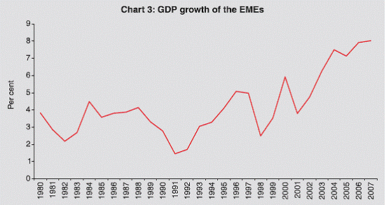
With the increase in capital flows, particularly private capital flows, the growth of EMEs has increased substantially signaling about the positive relationship between financial openness and economic growth. As can be observed from Figure 3, GDP growth rates were high during mid-1990s and in the current 21^st century when the capital flows to EMEs were significantly large. However, both the capital inflows and growth were lower in 2008 mainly due to global economic and financial crisis.

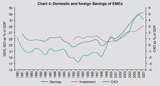
Though it is true that GDP growth remained high during the phases of heavy capital flows, it is not clear whether capital inflows increased growth in EMEs. Findings of many studies show that capital inflows used to be high during the phases of high economic growth and they are procyclical in nature. It has been justified that capital account liberalization by fulfilling the investment demand in capital poor countries enhances economic benefits. However, a converse can be observed from Figure 4 that EMEs have higher saving rates than investment rates during 2000s.

The same can be confirmed from the positive current account balance reflecting net exporter of capital. Therefore, the immediate question is whether the EMEs need capital inflows at all and if they require, how effective is capital flows for them in achieving their goals. As mentioned above, it may be possible that higher growth in the EMEs attracting capital flows. However, as can be observed from a scattered regression plot for select 27 emerging countries given in Figure 5 that there is a positive relationship between per capita GDP growth and financial openness⁶. It may be possible that productivity growth led by financial globalization has been impacting GDP growth. Thus, it is relevant to study the relationship between capital flows and economic growth in EMEs. To examine this issue we tried to study the long-run linkages of financial openness and per capita GDP.

Section IV
Data and Methodology

Financial Globalization or financial openness (FINOP) in this study is measured as the net capital flows to GDP ratio⁷. The net flows are net of financial account excluding official reserves, i.e. the credit less debit of financial account of balance of payments of the emerging market countries. The choice of the data period for the empirical analysis is based on the availability of data on net capital flows, i.e. for the period 1980 through 2007. Per capital GDP (PGDP) used in the study is calculated taking real PDGP growth rates and GDP for 1980 dividing total population in that year. Other variable used in the paper is trade openness (TROP) measured as the sum of merchandised exports and imports as a share of GDP. Net capital flow, exports and imports data are collected from Balance of Payment Statistics of IMF CD-ROM and the GDP, per capita GDP growth rates, population data are taken from World Bank online database. The choice of countries in the EMEs is based on the MSCI classification of emerging market economies plus Saudi Arabia. The data used in the study are for 27 countries⁸ for the period 1980-2007 resulting total 756 observations. L is pre-added when the variables are in natural log forms, e.g. LPGDP for log of PGDP.

Methodology

Model:

We have used standard neo-classical growth model where the output per capita (Y) is a function of capital per labour (K) in Cobb- Douglas form:

where A₀ is the initial stock of knowledge. In a standard Solow model, total factor productivity (TFP) is autonomous, in the longrun, steady state growth equals g. The alternative specifications, where TFP is assumed to dependent on FINOP i.e., g = g(FINOP) in a linear form, as follows.

Taking log in both sides:

In the equation (3) output per capita increases with the increase in financial globalization and increase in capital-labour ratio over time.

We have estimated a simplified version of equation (3) and considered the panel method with cross section (i=1,2 …27) and time period (t=1,2 …28) dimension:

Econometric Framework⁹:

Like timeseries data, the panel data with longer time dimension needs to qualify for the stationarity tests. The recently developed panel-based unit root tests by Levin, Lin and Chu (2002), Breitung (2002), Maddala and Wu (1999), Hadri (1999), and Im, Pesaran and Shin (2003) are similar to tests carried out on a single series. Interestingly, these investigators have shown that panel unit root tests are more powerful (less likely to commit a Type II error) than unit root tests applied to individual series because the information in the time series is enhanced by that contained in the cross-section data. We have applied all the above mentioned unit root tests to examine the stationarity of the panel data used in the study.

Recently developed panel cointegration techniques, viz. Pedroni cointegration test (1999 and 2004), Kao cointegration test (1999) and Maddala and Wu cointegration test (1999) were applied to test the long-run relationship between variables in above equation (4).

Section V
Empirical Analysis :

To test the stationarity of the variables, the panel unit root tests conducted in level as well as with first difference and the results are reported in Table 2. The results show that the variables LPGDP and TROP are I(1) in levels and I(0) in first differences. LPGDP is nonstationary at level as both LLC and IPS tests could not reject the null hypothesis of having a unit root and Hadri test rejects the null of not having a unit root. In case of trade openness (TROP), LLC, Breitung, IPS and MW statistics confirmed that the null of having a unit root could not be rejected; and null of no unit root in the data were rejected as the Hadri Z statistics rejects the null hypothesis. In contrast, except Hadri test, all the tests show that FINOP is stationary at level. However, all the variables are stationary at the first difference.

To confirm the order of integration of the variable FINOP, we have also conducted intermediate ADF unit root tests for each cross-section as can be generated from IPS tests. The test results are presented in Table 3. The results witnessing unit roots in several country cases and average t-statistics is insignificant indicating to have a unit root in FINOP in level. Therefore, we assume that FINOP is an I(1) process. Thus, the evidence suggests that the variables in question do evolve as non-stationary processes and the application of OLS (or GLS) to the equation (4) will result in biased and inconsistent estimates. Therefore, it is necessary to turn to panel cointegration techniques to examine the existence of a long-run equilibrium relationship among the non-stationary variables in level form.

We proceed to check for cointegration between the variables in equations (4), and also including another variable trade openness (TROP) in that equation through the tests proposed by Pedroni (1999 & 2004), Kao (1999) and Maddala and Wu (1999). Pedroni cointegration tests have four panel statistics and three group panel statistics. In the case of Pedroni’s panel statistics, the first-order autoregressive term is assumed to be the same across all the cross sections (within cross sections), while in the case of group panel statistics the parameter is allowed to vary over the cross sections (between cross sections). On the contrary, Kao’s test assumes homogeneous cointegrating vectors and autoregressive coefficients. The results of Pedroni and Kao cointegration tests are reported in Table 4. The results in Table 4 show that the null of no cointegration is rejected as all test statistics are significant. All the four panel test and three group test – statistics are significant suggesting that there is a cointegrating relationship between per capita GDP and financial openness both in within the cross-section and between cross-sections. When trade openness included in the equation, the result remained unchanged. Similarly, the ADF t-statistic from Kao’s cointegration test shows that there is a long-run relationship between per capita GDP and financial liberalization with the rejection of null of no cointegration. Inclusion of trade openness, in fact, increases the significance of t-values indicating a relationship among per capita GDP, financial openness and trade openness.

The study also employed a Johansen cointegration test using the methodology proposed by Maddala and Wu (1999). Using Fishertype test, Maddala and Wu proposed an alternative approach to test cointegration in panel data by combining tests from individual of Madala and Wu cointegration test using an underlying Johansen methodology are provided in Table 5. The results corroborated our earlier findings by confirming at least one cointegrating vector exists between the PGDP and FINOP as both the trace and maximum-eigen test statistics are significant at 1 per cent level.

Panel DOLS and FMOLS Estimates

Having established that there is a cointegrating relationship exists between the variables, the long-run estimates of the equation (4) can be obtained using fully Modified ordinary least square (FMOLS) and dynamic ordinary least square (DOLS). In order to estimate long run coefficients of the cointegration relationship (g₂), we use FMOLS and DOLS between-dimension approach proposed by Pedroni (2001) as the conventional OLS estimator is a biased and inconsistent estimator when applied to cointegrated variables¹⁰. The FMOLS estimator not only generates consistent estimates of the β (g₂ in our study) parameters in small sample (in our case 27 years), but it controls for the likely endogeneity of the regressors and serial correlation. Further, an important advantage of the between-dimension estimators is that the form in which the data are pooled allows for greater flexibility in the presence of heterogeneous cointegrating vectors.

The results of DOLS and FMOLS regression estimates for individual countries are reported in Table 6 and 7. The estimation is also conducted to capture common shocks through common time dummies¹¹. As can be observed from the Table 6, FMOLS and DOLS estimates are significant for most of the countries. Further, the coefficients of the FINOP are significantly positive for many countries and significantly negative for only few countries. With capturing common shocks to the countries, the results remained almost indifferent.

Table 7 provides slope coefficients of FINOP controlling for trade openness (TROP). It is interesting to observe that the coefficients of FINOP for many countries turned positive. Further, the significance level of few countries, which were earlier less, has increased now. The coefficients of TROP are positively significant for most of the countries.

The results for panel Group-Mean DOLS and FMOLS with and without common time dummies are reported in Table 8. Further, the results are also reported in Panel B controlling for trade openness. In all the cases, the cointegrating coefficient, i.e. the coefficient of the FINOP is significantly different from zero. The coefficients of TROP are also significantly positive as expected in the theory that trade openness has positive impact on growth. In Panel A, the coefficient of FINOP is significant and positive both including common time dummies and without including common time dummies. Further, magnitude of the coefficients though varied with dummies and without dummies, it remained more stable in case of FMOLS. The results in Panel B are different from that in Panel A. Without time dummies, the DOLS estimates of FINOP coefficient is positive while FMOLS estimates of the FINOP coefficient is negative. Capturing the impact of common shocks to the countries in the panel through common dummies, the DOLS coefficient of FINOP remained unchanged but significant level has increased. The FMOLS coefficient of FINOP turned positive and significant level is also higher than that in the without dummy case. As we have also seen in the individual case, the significance level of the coefficients of FINOP is higher controlling for common shocks. This result with common time dummies is more reliable as it excludes the impact of common shock that are shared across individual members. Therefore, the result with common dummies has higher significance level as it is free from any common disturbance affecting our results in earlier case. The coefficient of FINOP is significantly positive in DOLS and FMOLS in most of the cases. This means, financial globalization has positive impact on growth. We have also found that the impact of trade openness on growth is positive.

Section VI
Concluding Remarks :

This study, in a unique way, examined the long-run relationship between economic growth and financial liberalization for select 27 EMEs. Unlike other studies in the literature, the study is able to use recently developed panel unit root test and cointegration test on the basis of neoclassical theory of economic growth, which links capital account liberalization with level of per capita output instead of per capita output growth. Using the cointegration tests as proposed by Pedroni, Kao and Maddala and Wu, we found that there is a dynamic long-run relationship exists between economic growth and financial openness. The results are also remained unchanged when we have controlled for trade openness contribution to per capital GDP. Further, the long-run coefficient of financial openness is estimated through panel DOLS and FMOLS, which is significantly positive. The findings are interesting to show a positive long-run relationship exists between capital account liberalisation and growth as opposed to the findings of many earlier studies.

Notes:

* Authors are Research Officer and Director, respectively, in the Department of Economic Analysis and Policy, Reserve Bank of India. The views expressed in this paper are those of the authors and not of the institution to which they belong.

¹ Financial globalization, financial liberalization and financial integration are used interchangeably in this paper referring to the cross border trade of financial assets as well as deregulation of the capital account to increase foreign investors’ participation in domestic financial markets and domestic investors’ participation in the financial markets of the rest of the world.

² However, there was slowdown in capital inflows to EMEs with the onset of the recent global financial crisis.

³ On contrary, a recent trend shows that capital flows from rich to poor countries.

⁴ Behera, HK (2008) Does Financial Globalisation Spur Growth in India? A Paper presented in the 44th Annual conference of The Indian Econometric Society during January 3-5, 2008.

⁵ The trend reversed as a consequence of global financial crisis starting with Lehman failure in September 2008.

⁶ A discussion about the selection of 27 EMEs is given in section IV and Appendix I.

⁷ Net capital flows rather than gross capital flows are used for defining Financial Globalization as net flows matters for a country’s investment point of view.

⁸ The list of countries in the EME classification is given in Appendix I.

⁹ A detailed analysis of panel unit root test and panel cointegration test are provided in Appendix II

¹⁰ See Appendix III for details about FMOLS and DOLS. More details are available in Kao and Chiang (1997), Mark and Sul (1999), Pedroni (2000), and Pedroni (2001).

¹¹ Common time dummies are incorporated in the panel DOLS and FMOLS estimations to pick up any possible shocks, such as the East Asian crisis, that might affect all the countries in sample so that to deal with cross sectional dependency.

Reference :

Breitung J (2000) The Local Power of Some Unit Root Tests for Panel Data. In: Baltagi B (eds) Advances in Econometrics. Vol. 15: Nonstationary Panels, Panel Cointegration, and Dynamic Panels. Amsterdam: JAI Press, 161–178.

Eichengreen BJ (2001) Capital Account Liberalization: What Do Cross- Country Studies Tell Us? The World Bank Economic Review 15: 341-365

Fisher RA (1932) Statistical Methods for Research Workers, 4th edn. Edinburgh: Oliver & Boyd.

Hadri K (2000) Testing for Stationarity in Heterogeneous Panel Data. Econometric J 3: 148–161.

Henry PB (2007) Capital Account Liberalization: Theory, Evidence, and Speculation. J of Econ Lit 45: 887-935.

Im KS, Pesaran MH, Shin Y (1997) Testing for Unit Roots in Heterogeneous Panels. Mimeo, Department of Applied Economics, University of Cambridge.

Im KS, Pesaran MH, Shin Y (2003) Testing for Unit Roots in Heterogeneous Panels. J of Econometrics 115: 53-74.

Kao C (1999) Spurious Regression and Residual-Based Tests for Cointegration in Panel Data. J of Econometrics 90: 1–44.

Kao C, Chiang M (1997) On the Estimation and Inference of a Cointegrated Regression In Panel Data. Working Paper, Department of Economics, Syracuse University.

Kose MA, Prasad E, Rogoff K, Wei S (2006) Financial Globalization: A Reappraisal. IMF Working Paper No. 189, International Monetary Fund.

Levin A, Lin CF (1992) Unit root Tests in Panel Data: Asymptotic and Finite-sample. Properties. UC San Diego, Working Paper 92-23.

Levin A, Lin CF, Chu C (2002) Unit Root Tests in Panel Data: Asymptotic and Finite-Sample Properties. J of Econometrics 108: 1–24.

Maddala GS, Kim IM (1998) Unit Roots, Cointegration and Structural Change. Cambridge University Press, Cambridge.

Maddala GS, Wu S (1999) A Comparative Study of Unit Root Tests with Panel Data and A New Simple Test. Oxford Bul of Econ and Stat 61: 631–52.

Mark N, Sul D (1999) A Computationally Simple Cointegration Vector Estimator for Panel Data. Ohio State University manuscript.

Mishkin FS (2005) Is Financial Globalization Beneficial? NBER Working Paper No. w11891

Newbery D, Stiglitz J E (1984) Pareto Inferior Trade. Rev of Econ Stud 51: 1–12.

Obstfeld M, Taylor AM (2004) Global Capital Markets: Integration, Crisis and Growth. Cambridge University Press, Cambridge.

Pedroni P (1999) Critical Values for Cointegration Tests in Heterogeneous Panels with Multiple Regressors. Oxford Bul of Econ and Stat 61: 653–70.

Pedroni P (2000) Fully Modified OLS for Heterogeneous Cointegrated Panels. Advances in Econometrics 15: 93-130.

Pedroni P (2001) Purchasing Power Parity Tests in Cointegrated Panels. Rev of Econ and Stat 89: 727–731.

Pedroni P (2004) Panel Cointegration; Asymptotic and Finite Sample Properties of Pooled Time Series Tests with an Application to the PPP Hypothesis. Econometric Th 20: 597–625.

Perrault J (2002) Private Capital Flows to Emerging Market Economies. Bank of Can Rev: 33-43

Quinn D (1997) The Correlates of Changes in International Financial Regulation. Am Polit Sc Rev 91: 531–551.

Reinhart CM, Reinhart VR (2008) Capital Flow Bonanzas: An Encompassing View of the Past and Present. In: Frankel J, Giavazzi F (eds) NBER International Seminar in Macroeconomics 2008, Chicago University Press for NBER, Chicago.

Rodrik D (1998) Who needs capital account convertibility? Princeton Essays in Intl Finance 207: 1–10.

Schmukler SL (2004) Financial Globalization: Gain and Pain for Developing Countries. Econ Rev, Federal Reserve Bank of Atlanta: 39-66.

Stiglitz JE (2008) Capital market Liberalization, Globalization and the IMF. In: Ocampo JA, Stiglitz JE (eds) Capital Market Liberalization and Development:Oxford University Press, New York: pp 76–100

Stiglitz JE (1989) Financial Markets and Development. Oxford Rev of Econ Pol 5: 55-68

Appendix I:
List of EME Countries

The choice of countries in the EMEs is based on the MSCI classification of emerging market economies plus Saudi Arabia. The data used in the study are for 27 countries, which are given below:

Appendix II :
Panel Unit Root and Cointegration Tests

Unit Root Tests

All panel unit root tests, viz. Im, Pesaran and Shin (1995, 2003), the Levin and Lin and Chu (2002) test and the Maddala and Wu (1999) tests are based on a Dickey-Fuller-type regression:

Levin, Lin and Chu (LLC) Test:

Levin and Lin (1992) proposed a unit root test, which allows for fixed effects and unit-specific time trends in addition to commontime effects (which may in practice be concentrated out of the equation). The unit-specific fixed effects are an important source of heterogeneity here since the coefficient of the lagged dependent variable is restricted to be homogeneous across all units of the panel. However, LLC has advantage over Levin and Lin test as it allows for heterogeneity of cross-sectional units. The LLC tests amount to

Im, Pesaran and Shin (2003) formulated their model under the restrictive assumption that T should be the same for all cross

Kao’s test imposes homogeneous cointegrating vectors and autoregressive coefficients, but it does not allow for multiple exogenous variables in the cointegrating vector. Another drawback is that it does not address the issue of identifying the cointegrating vectors and the cases where more than one cointegrating vector exists.

Pedroni’s Cointegration Tests

Pedroni (1999, 2000 and 2004) proposes several tests for cointegration in panel data models that allow for heterogeneous slope coefficients, fixed effects and individual specific deterministic trends. The test has advantage over the test procedure proposed by Kao by allowing multiple regressors, for the cointegrating vector to vary across different sections of the panel, and also for heterogeneity in the errors across cross-section units.

The panel regression model that Pedroni proposes has the following form:

The second category includes three tests based on pooling the ‘between’ dimension (averaging the AR coefficients for each member of the panel for unit root test on residuals) and the parameter is allowed to vary over the cross sections. In these tests, therefore, the averaging is done in pieces so that the limiting distributions are based on limits of piecewise numerator and denominator terms. These test statistics can be given as:

A major drawback of the above procedure is the restrictive a priori assumption of a unique cointegrating vector.

Appendix III :
Panel FMOLS and DOLS Tests

Fully Modified OLS (FMOLS) Mean Group Panel Estimator

The precise equation estimated with FMOLS can be derived from the following equation: