Snehal Herwadkar and Saurabh Ghosh* The phenomenon of heterogeneous credit distribution across Indian states is well documented in literature. This study contributes to existing research by evaluating whether this diversity can be attributed to the risk-return profile of the states. In particular, it evaluates whether credit inequality across Indian states can be explained by state specific factors representing credit demand and supply and infrastructure facilities. Evaluating data for 22 Indian states for 2004-12, this paper concludes that the differences in credit distribution can be explained by factors such as financial deepening and physical infrastructure development. This indicates that states which garner higher deposits, have better banking networks and score high on infrastructure availability attract more credit as compared to other states. These results highlight that from the policy perspective, while the role of financial inclusion is important, the states can also contribute towards this goal by providing better infrastructure facilities that would enhance the investment climate in the states. Policy efforts, therefore, should focus on these issues as well as on promoting the spread of the formal banking channel. JEL Classification : R1, G210 Keywords : Emerging Market Economies, India, Credit, Regional Diversity, Financial and Physical Infrastructure. Introduction The relationship between credit and economic growth and development has fascinated academics and practitioners alike. An old question continues to engage the economics profession deeply: does financial development promote growth or does economic growth propel financial development or is it both ways? (Patrick 1966, Gurley and Shaw 1967, Goldsmith 1969, Mckinnon 1973, Jung 1986, King and Levine 1993). This paper contributes to this still unsettled debate by asking: does higher economic growth and better banking, social and physical infrastructure attract more credit to a particular region relative to others? It draws heavily on the wider discussion in literature on the phenomenon of uneven credit distribution across regions in the context of development (Samolyk 1989 and Hassan et al. 2011 provide a comprehensive review). Ruling orthodoxies in the evolution of ideas on this theme – ranging from the neo-classical profit-driven redistribution approach to the productive sector hypothesis (Mydral 1957) to the Keynesian liquidity preference approach – assign a passive role to financial intermediation. By contrast, policymakers across developed and emerging market economies (EMEs) are increasingly analysing the contribution of factors like the maturity of the banking sector and developmental indicators in studying credit distribution across regions (Jayaratne and Strahan 1996). Can policy interventions influence regional credit distribution patterns? This paper attempts to shed light on this question by evaluating the Indian experience. Among EMEs, India provides an interesting test case given its heterogeneity in terms of geographic, economic, developmental and demographic characteristics across states. Using a large panel of 22 states and data for nine years (2004-12), we analyse the differences in credit distribution. The central question that we attempt to answer is: why does credit distribution differ so much across Indian states? Our hypothesis is that financial flows track highest risk-adjusted returns on investment. These returns differ across states due to various factors: availability of deposits, state of financial development, investment climate in the state, availability of infrastructure and transaction costs and ease of doing business, etc. The challenge of representing these factors through appropriate proxy variables is a multi-layered one because it is difficult to capture qualitative factors through quantifiable variables. Moreover, long time series for quantifiable variables are not always readily available. Notwithstanding these difficulties, we narrowed down to a set of key indicators which we think would adequately represent the unique characteristics of each state to carry out our analysis. These include: (i) state specific cyclical factors (that is, gross state domestic product –GSDP) and structural factors characterizing the state (that is, share of agriculture and services sectors in GSDP), (ii) major factors representing financial intermediation and deepening, for example, supply of credit (deposits from the state) or banking network proxied by bank centres, and (iii) proxies for existing infrastructure facilities and the law and order situation in a state, for instance rail density,1 electricity generation and criminal activities in the state. Empirical estimates employ an array of alternative models while adjusting for state specific effects. Our results suggest that apart from state GDP, financial networks and the availability of infrastructure are the major factors influencing credit disbursements across Indian states. The rest of the paper is organized as follows. Section II gives an overview of international and Indian literature. Section III elaborates on the data used in the study while Section IV describes empirical results and the main inferences. The final section summarizes the results, discusses the policy implications and indicates the way forward. Section II
Literature Survey Economics and finance literature is replete with studies investigating the inter-relationship between economic growth and credit. Authors like Mckinnon (1973), King and Levine (1993) Levine et al. (2000) and Rajan and Zingales (1998) have argued that financial development leads to more efficient allocation of resources, which ultimately translates into higher economic growth. On the other hand, authors like Gurley and Shaw (1967), Goldsmith (1969) and Jung (1986) have argued that higher economic growth creates demand for a better and more efficient financial sector and the financial sector merely fulfils this demand. Some authors have also found evidence of bi-directional causality (Blackburn and Huang 1998, Khan 2001 and Hassan et al. 2011). In the Indian context, Demetriades and Luintel (1996) have documented bi-directional causality while Chakraborty (2010) has found evidence that banking sector development promotes economic growth. As the causality between growth and financial development has been adequately explored in literature, we attempt to empirically quantify credit dispersion and factors such as fund supply and availability of financial and physical infrastructure that could help in explaining this diversity. International Experience The neo-classical theory postulates that free movement of factors of production will automatically result in an exodus of labour from an underdeveloped region to a developed region, while financial resources in pursuit of higher returns will seek more profitable opportunities available in an underdeveloped region. In such a system, banks may fail to allocate resources among different regions due to imperfect or asymmetric information or due to barriers to inter-regional movement of financial flows like transaction costs or policy requirements. This neo-classical postulation has been challenged by Myrdal (1957) and Prebisch (1962). Both the Myrdal’s ‘cumulative causation theory’ and Prebisch’s ‘dependence theory’ suggest that yields of productive factors may vary between regions and the risk adjusted profitability of capital is higher in developed regions. This results in the developed regions not only utilizing and exhausting all their financial resources, but also in attracting capital from less developed regions. In both the neo-classical and Myrdal-Prebisch postulations, financial intermediation and the banking sector play only a limited role, which is confined to garnering deposits and deploying these funds as credit. Later research in the theory of development phases of the financial system challenged the passive role assigned to the financial sector (Chick and Dow 1988 and Dow 1990). These theories indicate that as the banking system becomes more mature, it develops an ability to create credit in certain regions without reducing it in others. In this development phase, the decisions of the banking system to finance development activities in one region are independent of deposits at its disposal. Samolyk (1992) developed a regional credit model and its empirical application for the US, which suggested that local banking sector problems may constrain economic activity in financially distressed regions, whereas no such link was evident in financially sound regions. Gonzalez and Sales (2001) added to this strand of literature by highlighting the role of expectations about the number and magnitude of investment projects, which in turn determine the demand for financing or credit availability. The authors also found that in Spain the introduction of regional banks resulted in relatively low inter-regional differences. A study by the same authors done earlier found that the preference for liquidity was greater in the relatively lesser developed regions and in those that had a less promising economic outlook, which resulted in relatively lesser creation of credit for the region and an outflow of capital to more advanced regions. Lima and Resende (2008) found evidence among the EMEs of inequality in deposits translating into local credit for Brazilian states; moreover their study highlighted the role of bank group-wise differences (public versus private banks) in such an inequality pattern. There is hardly any study that explicitly analyses the role of infrastructure in analysing the credit disbursement pattern, at best it has been implicitly assumed in per capita income. Banos et. al (2011) studied the relationship between regional banking and economic development in the Philippines and found a positive link between regional indicators of economic development and banking development with a specific influence of rural banking mainly in the intermediate‐developed regions. For the less developed regions however, they found no evidence of commercial, thrift or rural banks contributing significantly to the economic development. Indian Literature There are only a handful of studies that address spatial divergence in credit distribution in India and the empirical evidence is mixed. While Das and Maiti (1998) found no significant evidence of credit migration, Tyagarajan and Saoji (1977) observed that credit migration was largely restricted to four major metropolitan cities. Pai (1970) showed that for industrially developed states, credit expansion was at a higher rate as compared to the deposit growth rate while the vice versa was true in case of industrially backward states. Chatterjee et al. (1997) observed that migration of credit in the major states had become more uniform between 1974 and 1994. Singh and Srinivasan (2006) analysed data on 14 Indian states for 1990-91 to 1998-99 and found that per capita bank credit was an important determinant of growth. They also found that credit deposit ratios and FDI approvals per capita had a positive impact on growth. Finally, they observed that C-D ratios (a proxy for the internal movement of capital) had both become more varied across states and more closely related with GSDP per capita over the period. They concluded that capital, both foreign and domestic, flows to regions where it can be more effectively used, namely in higher income states. This result is also corroborated by Chakravorty (2003) who found that there was a correlation between investment and determinants of profitability such as measures of physical infrastructure and distance to market area and to shipping hubs. In another strand of literature, Dhal (2012) found evidence which broadly corroborated asymmetry in credit and the bank lending channel of monetary policy transmission across different states. His findings suggest that poor states are likely to be more affected by a tight monetary policy. Contribution of the Present Study While the issue of inequality in the spatial distribution of credit is neither unique to India, nor a new concern, our study attempts to add to literature in two distinct ways. First, most of earlier studies have documented the regional disparity in credit but done little analysis of the macroeconomic factors behind the regional disparity in credit. To explain variations in credit distribution across states, taking a cue from the recently available literature, we include a large number of variables in our empirical analysis that have not been used in the Indian context. Second, earlier studies relating to India on this subject selected bigger states, completely ignoring the smaller ones. However, since this study is about explaining asymmetry in credit distribution, it is important not to exclude small states out of the sample, as that could distort the analysis. We, therefore, use a large number of states (22); only some union territories and certain states in the north-eastern region could not be covered in the study due to non-availability of consistent time series data. Section III
Data Our study employs panel data on 22 Indian states2 for the period 2004-12. As most of the variables are available only with an annual frequency our study uses annual data. Data for this study was culled from a variety of sources. State-wise time series data on outstanding deposits and credit and bank centres of scheduled commercial banks were taken from the Basic Statistical Returns (BSR) dataset of the Reserve Bank of India. Variables like gross state domestic product, state per capita income, fiscal deficit to GDP ratio of states, share of non-industry, agriculture and services in state domestic product, factories in operation, infrastructure facilities and proxies for law and order situation in state (such as electricity generation, power deficit, crime rate, conviction rate and rail and road density) were taken from the Centre for Monitoring Economy (CMIE) database on the states of India. Non-availability of data on infrastructure facilities before 2004 has constrained the time period under consideration. A summary and definitions of all the variables is presented in Annexure I. Credit growth across Indian states has varied substantially in terms of average growth rates and their time path (Chart I and V). An analysis of the share of states in all-India credit points to stark contrasts (Chart II and VI). We also considered a third variable, the credit to GSDP ratio to represent state credit distribution as a percentage of economic activity to take care of the size of the state. Here again, only a few states showed high credit to GSDP ratio, but most of the states had low levels of the ratio (Chart III and VII). As is evident from these charts the variables representing credit distribution did not follow a similar path across states and their locus varied considerably over time. Section IV
Empirical Estimation and Analysis i) Credit growth convergence Before analysing the factors explaining credit divergence across states we attempt to evaluate whether there has been a convergence in credit growth across states over the years. To empirically investigate the presence of credit disparity across Indian states, the β-convergence method was used. The fixed effect panel regression consisted of 22 major states for 2004-12 with nine year average credit growth as a dependent variable and the base period credit growth as an independent variable. The coefficient of β was found to be positive and statistically insignificant at the conventional level. This finding suggests no statistically significant evidence of convergence of credit growth across states over time. ii) Panel regressions Having established significant divergence in credit off-take across states and insignificant convergence in them, we now attempt to identify some of the factors that could help in explaining the persisting divergence across Indian states. The list of variables used to explain credit divergence across states and their economic rationale is now discussed. In line with the arguments extended by various authors including Gurley and Shaw (1967), Goldsmith (1969) and Jung (1986), we examine whether the high growth of a particular state helps in attracting more bank credit to that particular state and vice versa. Second, amongst the three sectors of agriculture, industry and services, the share of industry in non-food credit in India has always remained the highest. However, since there have been studies relating the industrial sector to credit distribution and in view of the recent emphasis on financial inclusion and SMEs, we considered the share of the non-industrial sector in gross state domestic product to represent the comparative size of the agriculture and services sectors in a state. Further, state deposit is taken as a proxy representing the resources available to the financial sector for its lending activities in line with the argument proposed by Beck et al. (2009) and Resende (2008). In today’s world of a technology driven banking sector, deposits garnered from a particular region need not be a constraint in extending credit to that particular region. However, the deposit base of a particular region can also be taken as a proxy of the presence of the banking sector in the region. It is clear that higher the penetration of the banking sector in a region, greater would be the credit extended through formal channels. We also considered banking centres which are taken as representative of the level of financial deepening in the state. One of the key features of this paper is the introduction of infrastructure proxies as explanatory variables for state credit. The crucial role played by infrastructure in economic development has been well established in academic literature for a long time (Hirschman 1958 and Rostow 1960). Better infrastructure facilities like transport, communication and power help in enhancing the productivity of investment in that region, which in turn propels competitiveness. Availability of trade infrastructure like ports, highway corridors and railroads reduce transportation costs, facilitate smoother mobility of people and products and help in easing productivity constraints. These gains are often experienced over a long period of time rather than in the short term. Thus a state which has created an enabling environment through infrastructure facilities is likely to attract more investment and in turn more credit, notwithstanding its present growth or level of GDP. Taking into account infrastructure factors, we account for the expectations about the number and magnitude of investment projects, which in turn determine the demand for financing or credit availability in line with the argument extended by Gonzalez and Sales (2001). We employ a generic panel data model with credit (or its transformation) as a dependent variable and function of gross state domestic product, share of non-industry, deposit accumulation, bank centres, railway, electricity generation and crime as independent variables. All the explanatory variables have been suitably standardized taking into account the size of the state. The equations are: G(credit)it = f(GSDP(t-1), share_nonindustryit, depositit, bank_centreit, railit, electricityit, crimeit)+ αi + λt + εit Where G(.),f(.) are functions such as log, difference or ratios, while εit is assumed to follows normal distribution. Before analysing data for panel regression, we consider evaluating their properties, by running Levin-Lin-Chu Test (LLC) test, which tests the hypothesis H0: each time series contains a unit root against H1: each time series is stationary. The finding of this procedure is reported in Table 1. | Table 1: Panel Unit Root: Levin, Lin & Chu Test (Null: unit root) | | | Statistic | Prob. | sections | Obs | | Log(credit) | -8.89 | 0 | 22 | 154 | | log(deposit) | -3.91 | 0 | 22 | 154 | | log(bank_centres)* | 16.15 | 1 | 22 | 154 | | log(Rail)* | 0.07 | 0.54 | 18 | 126 | | log(electicity) | -0.66 | 0.25 | 22 | 153 | | Power_Deficit | -7.17 | 0 | 21 | 121 | | log(crime) | -7.23 | 0 | 22 | 154 | | Note: *: variables found to be difference stationary. | In the following section, we use different indicators of state-wise outstanding credit (both in levels and in standardized form). We start with level of credit (as it was found stationary) and estimate coefficients of deposit, banking network and other infrastructure variables. We controlled for gross state domestic product (GSDP) for the size and cycles of economic activity in the state. However we used one period lagged value of GSDP to avoid an endogeneity problem. The model with cross-section and period fixed effect was chosen on the basis of the F-statistics and redundant fixed effect chi-square test statistics. The estimated coefficients are reported in Table 2 (Model-1). As some of the variables (for example, bank centres, railways and electricity generation) were found to be unit root process, we replace them by first difference (D(Rail) and D(bank_centres)) and by power_def. The cross-section and period fixed effect model was identified by the redundant fixed effect likelihood ratio test; their coefficients are reported in Table 3 (Model-2). In both of these estimates, the coefficient diagnostics clearly rejected the null of redundancy of financial inclusion variables and infrastructure variables; the coefficient and their significance indicate a strong positive relationship between credit with deposit mobilization and change in the number of banking centres in line with Beck et al. (2009) and Resende (2008). Further, among the infrastructure variables, increase in railway operational routes had a positive coefficient (Model-2). Power deficit had a positive coefficient, which could indicate increase in the cost of production in the deficit states; however it is only significant at the 10 per cent level. | Table 2: Panel Estimates Explaining Credit Disbursement | | Variable | Coefficient | Prob. | Coefficient | Prob. | Coefficient | Prob. | | Cross & Time Fixed | Cross & Time Fixed | Panel GMM | | Model-1 | Model-2 | Model-3 | | log(credit(-1) | | | | | 0.28 | 0.42 | | C | 4.72 | 0.04 | 0.75 | 0.71 | | | | L_DEPOSIT | 0.13 | 0.09 | 0.19 | 0.08 | 0.42 | 0.35 | | LOG(BANK_CENTERS) | 0.74 | 0.00 | | | | | | DLOG(BANK_CENTERS) | | | 0.71 | 0.05 | 2.85 | 0.19 | | L_SDP(-1) | 0.19 | 0.07 | 0.69 | 0.00 | 1.26 | 0.04 | | SHARE_NonIND | 0.001 | 0.65 | 0.003 | 0.43 | 0.01 | 0.42 | | LOG(RAIL) | -0.67 | 0.00 | | | | | | LOG(ELECTRICITY) | 0.07 | 0.06 | | | | | | LOG(CRIME) | -0.01 | 0.69 | | | | | | DLOG(RAIL) | | | 0.26 | 0.05 | 0.01 | 0.97 | | POWER_DEF | | | 0.003 | 0.10 | -0.003 | 0.74 | | CONVICTION_RATE | | | -0.0003 | 0.68 | 0.01 | 0.11 | | R2 | 0.97 | | 0.98 | | 0.20 | | | Arellano Bond AR(2) | | | | | | | | M-stat | | | | | 0.01 | | To evaluate the persistence of credit flows or lag dependence of the state credit factor, we included first lag of credit in the equation and estimated this dynamic model in the Panel GMM framework, using the Arellano–Bond two-step procedure. Here 2-period lagged value of credit was used as an instrument for GMM estimation. However, the estimation results indicate (Table 3, Model-3) that the coefficient of the lagged credit variable was not significantly different from zero, the R-square value was low and finally the Arellano-Bond second lag autocorrelation was found to be serially correlated, indicating that the dynamic panel is not a good fit in this context. Indian states vary considerably in terms of their size, population and sectoral activities. So it is expected that the absolute level of credit disbursement would be different across states. Empirically, in the fixed effect panel regression, the state specific scale effect is likely to be addressed by cross-section fixed dummies. However, to address the scale effect explicitly we used different transformations of credit disbursement, which include state credit as a ratio of all India credit (credit_ai), state credit as a ratio to state GDP (credit_gsdp) and credit growth rate (Gr_credit).3 The deposit and GSDP was appropriately standardized. For instance, for estimating credit_ai, credit_gsdp and credit_gr we used state deposit to the all-India deposit ratio, state deposit to GSDP ratio and deposit growth respectively. Using each of credit_ai, credit_sdp and credit_gr as dependent variables and appropriately normalized set of independent variables, we estimated three sets of panel regressions (Table 3). The results indicate that deposit mobilization and the banking network play an important role in credit creation in a particular state. This emphasizes the role of financial sector inclusion and development in credit creation and is in line with the findings of Love (2003). The coefficients of increase in rail network remain positive (except for credit growth equation), state power deficit has a positive coefficient, and conviction rate has a positive and significant coefficient (Model-6). The positive coefficient of power deficit (Model-4) though counter-intuitive could indicate shortage of power in the credit-starved industrial states or increase in the cost of production due to power shortage; in either case it calls for more infra-investment in the power sector. | Table 3: Panel Estimate Explaining Credit Dispersion Ratios | | Variable | State Credit to all India Credit | State Credit to GSDP | State Credit Growth | | Coefficient | Prob. | Coefficient | Prob. | Coefficient | Prob. | | Cross & Time Fixed | Time Fixed Effect | Time Fixed Effect | | Model-4 | Model-5 | Model-6 | | C | 0.24 | 0.47 | -0.42 | 0.00 | 11.76 | 0.01 | | LOG(DEP_AI) | 0.22 | 0.07 | | | | | | DEP_GSDP | | | 0.68 | 0.00 | | | | DEP_Growth | | | | | 0.20 | 0.04 | | DLOG(BANK_CENTERS) | 0.90 | 0.02 | 2.21 | 0.00 | 17.29 | 0.43 | | GSDP_AI(-1) | 0.15 | 0.00 | | | | | | GR_GSDP(-1) | | | | | 0.06 | 0.53 | | FD_GSDP | | | -0.04 | 0.00 | | | | SHARE_NonIND | 0.0004 | 0.92 | 0.01 | 0.00 | 0.03 | 0.58 | | DLOG(RAIL) | 0.27 | 0.06 | -0.09 | 0.74 | -33.53 | 0.00 | | POWER_DEF | 0.01 | 0.02 | 0.0003 | 0.87 | 0.09 | 0.13 | | CONVICTION_RATE | -0.0001 | 0.24 | 0.0001 | 0.86 | 0.04 | 0.01 | | R-square | 0.97 | | 0.84 | | 0.46 | | | Note: Models selected on the basis of Redundant Fixed effect likelihood ratio test. | The share of the non-industrial sector seems to have a positive influence (Model-5) on share of credit to state GDP indicating that the states with a larger share of agriculture and services sectors attract more credit relative to their GSDP. One reason could be that in the recent period the services sector has emerged as the engine of growth for the Indian economy. In the equation explaining credit to GSDP, fiscal deficit as a per cent of GSDP had a negative and significant coefficient indicating the adverse impact of a large state deficit on credit distribution. In line with research by Blejer and Khan (1984), this result suggests that the higher level of fiscal deficit may be ‘crowding out’ private investment. Finally, in almost all of the estimated equations, coefficients of the one- period lagged GSDP variable are positive and significant indicating the positive impact of state GDP on credit disbursements.4 All estimated models include year dummies to control for year specific effect, including that of business cycles, interest rate movements or global financial crises that uniformly affect bank credit disbursement across states. A plot of these time dummy coefficients, which were found to be jointly significant, clearly indicates two phases of credit cycle with a break around the global financial crisis (Chart IV). The residual diagnostics confirmed normal distribution of the panel regression errors. In an attempt to test the robustness of our findings and address the possibility of some of the important variables of interest being omitted, we attempted modeling with a large number of alternative variables. These variables include corporate profit, new investment and per capita income as reported in the Annual Survey of Industries (ASI) and the National Accounts Statistics (NAS) database. We also included infrastructure facilities like telecom and road infrastructure in a state as also the existence of port (dummy) in a state. However, these variables either had a multi-collinearity problem, as indicated by a near-singular matrix inversion problem or were found to be statistically insignificant in the omitted variable likelihood ratio test. The non-availability of longer time series especially relating to physical and social infrastructure constrains our analysis. Specifically, data on power deficit and conviction rate are available from 2004 onwards, which necessitated that the present analysis be restricted to nine years. A longer time series on these variables will be helpful in extending the analysis more fruitfully. A note of caution is also in order while interpreting these results. Some of the state specific variables showed substantial volatility across time and across states. A more robust dataset would be helpful in further strengthening the results. Section V
Conclusions Heterogeneity of credit distribution across regions has been attracting considerable academic and policy attention for a long time. While the studies so far have only documented credit heterogeneity across Indian states, our main objective was to examine factors that may explain some of the observed divergence. India provides a natural laboratory for studying heterogeneity given the considerable regional differences in terms of income, financial inclusion and infrastructure development. Using data from a large number of Indian states from 2004 to 2012, after appropriately controlling for cross-section and time specific effects, empirical evidence suggests availability of funds (deposits) and the banking network as the most important variables explaining heterogeneity of credit disbursement. Among infrastructure facilities, rail and power deficit emerge as factors that affect credit disbursement. State GDP and fiscal deficit are also found to be important factors influencing credit disbursements. These results motivate a few important policy implications. First, financial deepening is crucial, which not only helps in garnering more resources from the state but also helps in channelizing more resources to the state. The Reserve Bank’s recent policy initiatives such as setting up differentiated banks (such as payments banks) with a primary focus on the provision of basic financial services using new technologies could be helpful in achieving greater financial inclusion. The policy vision is to promote the spread of the formal banking channel, which will give impetus to formal credit lines, thus providing support to the growth aspirations of all the states. The government’s Jan Dhan Yojana to provide a bank account for each poor Indian family, where each account would include a debit card, accident and life insurance coverage and an overdraft facility is also a major step in this direction. Second, this paper also emphasizes the importance of infrastructure in explaining credit diversity across states. Providing better infrastructure to create an investor friendly environment and reining in the fiscal deficit of the state at the same time are factors that play an important role. 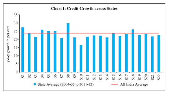 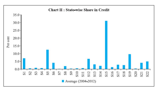 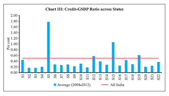 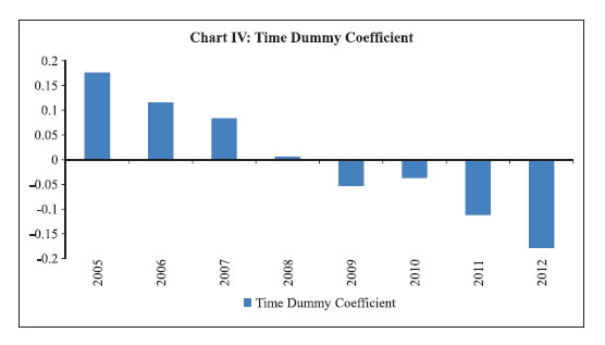 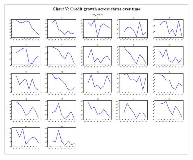 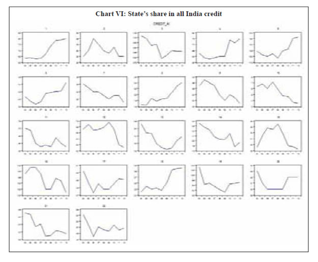 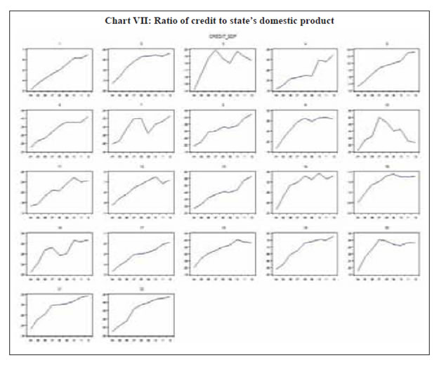
| Table 1: Summary Statistics of the Variables | | Dependent Variables | Definition | Source | Mean | Median | Maximum | Minimum | Std. Dev. | Skewness | Kurtosis | | CREDIT | Outstanding credit of SCBs (₹ Billion) | BSR, RBI | 1143.43 | 464.95 | 14046.74 | 22.81 | 1952.92 | 3.8 | 20.0 | | L_CREDIT | Log of credit | Authors’ calculations | 13.0 | 13.0 | 16.5 | 10.0 | 1.4 | 0.1 | 2.4 | | CREDIT_AI | Share of state in all India credit (per cent) | Authors’ calculations | 4.5 | 2.4 | 33.5 | 0.2 | 6.7 | 3.0 | 12.2 | | CREDIT_SDP | Credit to state GDP ratio | Authors’ calculations | 0.5 | 0.3 | 2.3 | 0.1 | 0.4 | 2.8 | 11.0 | | GR_CREDIT | Credit Growth | Authors’ calculations | 20.6 | 20.3 | 41.6 | -3.1 | 6.6 | -0.3 | 4.8 | | Explanatory Variables | | DEPOSIT | Outstanding Deposit of SCBs (₹ Billion) | BSR, RBI | 1547.51 | 869.84 | 15298.67 | 104.94 | 2169.65 | 3.7 | 20.0 | | BANK_CENTERS | Centres with atleast one branch | BSR, RBI | 1564.3 | 1474.0 | 5497.0 | 67.0 | 1124.5 | 1.2 | 5.0 | | GSDP | Gross State Domestic Product | CMIE, SOI | 1870461.0 | 1354055 | 10827513.0 | 88194.0 | 1719398.0 | 1.9 | 8.2 | | SHARE_NONIND | Share of agriculture and services sector in net state domestic product | CMIE, SOI | | | | | | | | | RAIL | Operational Railway route length in KM | CMIE, SOI | 27.4 | 21.7 | 138.5 | 0.4 | 24.7 | 2.9 | 12.4 | | ELECTRICITY | Electricity Generation (Mkwh) | CMIE, SOI | 30512.6 | 23828.0 | 97008.0 | 277.0 | 25704.1 | 0.8 | 2.7 | | CRIME | Cognizable Crime under IPC (nos./million) | CMIE, SOI | 4854.5 | 3179.0 | 20369.0 | 879.0 | 3908.4 | 1.4 | 4.5 | | POWER_DEF | Power deficit (per cent) | CMIE, SOI | -7.4 | -4.9 | 3.4 | -29.0 | 6.9 | -1.1 | 3.3 | | CONVICTION_RATE | Conviction rate (IPC) (per cent) | CMIE, SOI | 61.6 | 66.5 | 100.0 | 6.0 | 29.5 | -0.2 | 1.6 | | Transformed Variables | | DEP_AI | Share of deposit in all India | Authors’ calculations | 1.0 | 0.6 | 10.1 | 0.1 | 1.4 | 3.7 | 20.0 | | DEP_SDP | Ratio of Deposit to state net domestic product | Authors’ calculations | 0.8 | 0.6 | 2.9 | 0.3 | 0.5 | 3.0 | 12.5 | | GR_DEP | Growth of deposits | Authors’ calculations | 16.9 | 17.0 | 31.3 | -6.7 | 5.2 | -0.5 | 5.2 | | GR_SDP | Growth of state domestic product | Authors’ calculations | 14.3 | 13.8 | 26.2 | 0.6 | 4.6 | -0.1 | 3.3 | | FD_SDP | Ratio of fiscal deficit to state domestic product | CMIE, SOI | 3.6 | 3.2 | 11.3 | 0.5 | 1.8 | 1.4 | 5.7 |
References Baños, J., C. Crouzille, E. Nys and A. Sauviat (2011), ‘Banking Industry Structure and Economic Activities: A Regional Approach for the Philippines’, Philippine Management Review (Special Issue) 18: 97-113. Beck, T., A. Demirguc-Kunt and R. Levine (2009), ‘Financial Institutions and Markets across Countries and over Time: Data and Analysis’, Policy Research Working Paper 4943. The World Bank, May. Blackburn, K. and V. Huang (1998), ‘A Theory of Growth, Financial Development and Trade’, Economica 65(257): 107-24. Blejer, M. and M. Khan (1984), ‘Government Policy and Private Investment in Developing Countries’, IMF Staff Papers 31 (2): 379-403. Chakraborty, I. (2010), ‘Financial Development and Economic Growth in India: An Analysis of the post-reform period’, South Asia Economic Journal 11 (2): 287–308. Chakravorty, S. (2003), ‘Industrial location in post-reform India: Patterns of inter-regional divergence and intra-regional convergence’, The Journal of Development Studies 40 (2): 120-152. Chatterjee, A, K. Bhattacharya and S. Gayen (1997), ‘Migration of Credit Across States: An Empirical Investigation with Some New Measures’, Banking Statistics Division, Department of Statistical Analysis and Computer Services, Reserve Bank of India, Mumbai (mimeo). Chick, V. and S.C. Dow (1988), ‘A post-Keynesian Perspective on the Relation between Banking and Regional Development’, in P. Arestis (ed.), Post Keynesian Monetary Economics: New Approaches to Financial Modelling: 219-50, UK:Edward Elgar. Das, P. K. and P. Maiti (1998), ‘Bank credit, output and bank deposits in West Bengal and Selected States’, Economic and Political Weekly 33(47/48): 3081+3083-3088. Demetriades, P. and K. B. Luintel (1996), ‘Financial Development, Economic Growth and Banking Sector Controls: Evidence from India’, The Economic Journal 106(435): 359-74. Dhal, S. (2012), ‘A Disaggregated Analysis of Monetary Transmission Mechanism- Evidence from the Dispersion of Bank credit to Indian States’, in Deepak Mohanty (ed.), Regional Economy of India. Reserve Bank of India, Academic Foundation, New Delhi: 247-278. Dow, S. (1990), Financial Markets and Regional Economic Development: The Canadian Experience. Gower Publishers: Aldershot. Goldsmith, R.W. 1969. Financial structure and development, Yale University Press. Gonzalez, M. and Sales, J. 2001. ‘‘The spatial Distribution of Credit: The Case of Spanish Savings Banks’’. The Service Industries Journal, Vol. 21(4), pp.62-82. Gurley, J. and E. Shaw. 1967. ‘‘Financial Structure and Economic Development’’. Economic Development and Cultural Change, Vol. 15 (3), pp. 257-68. Hassan, M. K, B. Sanchez and J. Yu (2011), ‘Financial Development and Economic Growth: New Evidence from Panel Data’, The Quarterly Review of Economics and Finance 51 (1): 88-104. Hirschman, A. (1958), The Strategy of Economic Development. Yale University Press, Yale Studies in Economics. Jayaratne, J. and P. Strahan (1996), ‘The finance-growth nexus: Evidence from bank branch deregulation’,. The Quarterly Journal of Economics 111(3): 639–70. Jung, W. (1986), ‘Financial Development and Economic Growth: International Evidence’, Economic Development and Cultural Change, 34(2): 333-46. Khan, A. (2001), ‘Financial Development and Economic Growth’, Macroeconomics Dynamics 5(3): 413-33. King, R. and R. Levine (1993), ‘Finance and growth: Schumpeter might be right’, Quarterly Journal of Economics 108 (3): 717-37. Levine, R., L. Norman and T. Beck (2000), ‘Financial intermediation and growth: Causality and causes’, Journal of Monetary Economics, 46(1): 31-77. Lima, M. and M. Resende (2008), ‘Banking and Regional Inequality in Brazil: An Empirical Note’, Brazilian Journal of Political Economy 28 (4): 669-77. Love, I. (2003), ‘Financial development and financing constraints: Evidence from the structural investment model’, Review of Financial Studies 16(3): 765-91. McKinnon, R. I. (1973), Money and Capital in Economic Development. Washington, DC: The Brookings Institution. Myrdal, G. (1957), Economic Theory and Underdeveloped Regions. London: University Paperbacks, Methuen. Pai, G. A. (1970), ‘Regional Distribution of Bank Credit: A Critical View’, Economic and Political Weekly 5(41): 1691+1695-1699. Patrick, H.T. (1966), ‘Financial Development and Economic Growth in Underdeveloped Countries’, Economic Development and Cultural Change 14 (2): 174-89. Prebisch, R. (1962), ‘The Economic Development of Latin America and its Principal Problems’, Economic Bulletin for Latin America 7(1): 1-22. Rajan, R. and L. Zingales (1998), ‘Financial dependence and growth’, American Economic Review 88 (3): 559-86. Resende, M.L.M. (2008), ‘Banking and regional inequality in Brazil: an empirical note’, Brazilian Journal of Political Economy 28 (4): 669-77. Rostow, W.W. (1960), The Stages of Economic Growth: A Non- Communist Manifesto. Cambridge: Cambridge University Press. Samolyk, K. (1989), ‘The Role of Banks in Influencing Regional Flows of Funds’, Working Paper No. 9204, Federal Reserve Bank of Cleveland. Samolyk, K. (1992), ‘Bank Performance and Regional Economic Growth: Evidence of a Regional Credit Channel’, Working Paper No.9204, Federal Reserve Bank of Cleveland. Singh N. and T.N. Srinivasan (2006), ‘Indian Federalism, Economic Reform and Globalization’, in Jessica S. Wallack and T. N. Srinivasan (eds), Federalism and Economic Reform: International Perspectives. New York: Cambridge UP, pp. 301-63. Tyagarajan, M. and S.H. Saoji (1977), ‘Migration of Credit: An Aspect of Banking in Metropolitan Centres’, Reserve Bank of India Bulletin (December), pp. 802-13.
|