Rajesh Kavediya and Sitikantha Pattanaik* Volatility in the operating target of monetary policy could increase uncertainty about the cost of access to liquidity for any given policy interest rate, thereby pushing up the term premium and long-term interest rates. Empirical estimates of this paper indicate that conditional volatility in daily change in the Weighted Average Call Rate (WACR) - the operating target of monetary policy in India - exerts modest but statistically significant influence on volatility in daily change in other interest rates, namely nominal yields on government papers of three-month, six-month, nine-month, twelve-month, two-year and ten-year maturities. In the credit market, a one percentage point increase in WACR volatility (measured in terms of quarterly standard deviation) is estimated to cause about 26 basis points increase in bank lending rates. JEL Classification : E43, E52, E58 Keywords : Operating target volatility, Monetary policy transmission, Liquidity management Introduction The implementation of monetary policy has to often contend with episodic liquidity shocks and the associated risk of significant and sustained deviation of the operating target from the policy rate, notwithstanding proactive deployment of a variety of liquidity management tools by the Reserve Bank of India (RBI) to anchor the operating target close to the policy rate. The objective of minimising volatility in the operating target is largely conditioned by its potential ramifications on monetary policy transmission, and, therefore, the ultimate objectives of monetary policy. Long-term interest rates, which influence economic activity, reflect the expected future path of short-term interest rates, plus a term premium as compensation for uncertainty. One could argue that volatility in the overnight money market rates should not matter because economic decision-making in the real world would invariably be based on medium- to long-term interest rates (Cohen, 1999). The counter argument, which has shaped the designs of mainstream operating frameworks of monetary policies of major central banks, would suggest that lower volatility in the short-term overnight rates in the bank funding market could depress the term premium by limiting uncertainty about funding costs (Carpenter et al., 2016). The resultant lower medium- to long-term rates can influence economic activity. In empirical research, the causal influence of financial market volatility on macroeconomic outcomes is well-documented (Chiu et al., 2016). Unlike the short-run mean reverting component of volatility, the slow-moving long-run component often causes deterioration in macroeconomic fundamentals. An expansionary monetary policy has a much greater stimulating impact on output and employment in times of low-market volatility relative to periods characterised by high market volatility (Eickmeier et al., 2017). In the Advanced Economies (AEs), there is ample evidence of limited but statistically significant spillover of volatility from money market rates to long-term rates. Refinements in the operating frameworks over time, however, have reduced the scope for such spillover effects to very close to zero (Colarossi and Zaghini, 2009). Transparent operating frameworks and regular central bank communication on liquidity conditions have reduced uncertainty about the overnight money market rates, which has contributed to lower volatility of term rates (Osborne, 2016). Term rates, as opposed to overnight rates, are important to transmission. Therefore, central banks try to clearly communicate their views on the macro-financial outlook, so that the risk of uncertainty-induced volatility in the term premium is minimised. Aversion to volatility in long-term rates has even motivated researchers to put volatility in long-term bond yields explicitly in the objective functions of central banks (Stein and Sunderam, 2017). Unlike the AEs, in Emerging Market and Developing Economies (EMDEs) stronger and persistent volatility transmission from the overnight rates to long-term rates is observed, particularly during the transition to a more forward-looking inflation targeting regime, which highlights the importance of a stronger commitment to the operating target in these countries while implementing monetary policy on a day-to-day basis (Alper et al., 2016). Interest rate volatility has also been found to be a source of an upward pressure on spreads charged by banks over deposit rates while lending (Brock and Suarez, 2000). An operating framework of monetary policy that can dampen volatility on a sustained basis, during both normal and exceptional times, is therefore congenial to monetary policy transmission. If long-term rates are higher due to increased volatility in the operating target, then monetary policy can be viewed as tighter than actually intended while setting the policy rate (Carpenter et al., 2016). In other words, volatility in the operating target is not internalised, but transmitted to rates that matter for consumption and investment decisions (Ayuso et al., 1997). Monetary policy, though assessed often in terms of the current policy rate, is more about managing expectations about future short term rates. Therefore, transparent communication on the central bank’s macroeconomic outlook and its objective function is an important component of the modern-day monetary policy frameworks. The operating framework, which sub-serves the monetary policy framework and the monetary policy stance can enhance the effectiveness of monetary policy by minimising uncertainty about liquidity conditions that are critical to the overnight and short-term money market rates on a day-to-day basis. In India, after the announcement of demonetisation on November 8, 2016, there was a surfeit of surplus liquidity in the banking system, which exerted a sustained downward bias to the overnight money market rates. In an easing cycle of the monetary policy that started in January 2015 (with a cumulative cut in policy repo rate by 200 bps), any increase in volatility in the operating target could have dampened the transmission of monetary policy to the lending rates. Against this setting, an important research question is to empirically examine the role of volatility in the operating target in influencing long-term interest rates, and, therefore, the effectiveness of transmission. Section II sets out how the operating framework of monetary policy has evolved in India over time to, inter alia, minimise volatility in the operating target, while also responding to the exceptional liquidity shocks like demonetisation by using a mix of conventional and unconventional instruments of liquidity management. Section III discusses the research methodology and empirical results. Key findings and policy inferences are presented in Section IV. Section II
The Operating Framework of Monetary Policy in India Unlike monetary policy, which is about setting the appropriate policy interest rate based on a comprehensive assessment of macro-financial conditions and the outlook to achieve the mandated objectives, the operating framework is about day-to-day implementation of monetary policy and involves conducting appropriate liquidity management operations to ensure the first leg of transmission. Liquidity forecasting – or how the reserve demand of the banking system will behave ahead over successive days – is a critical component of the operating framework to guide the choice of relevant instruments for liquidity management as well as the timing of liquidity operations. While much of the normal overnight and term operations of the central banks draw on their liquidity forecasts, intra-day reassessment of liquidity conditions often guide fine-tuning operations. All such liquidity management operations aim at anchoring the operating target close to the policy interest rate, but that does not rule out its possible deviations from the policy rate, and the scope for time-varying volatility. In India, the post-global financial crisis liquidity scare, post-taper tantrum liquidity shock, and post-demonetisation liquidity glut, are the major instances when the RBI had to use exceptional liquidity management measures to align the operating target with the monetary policy stance. The following have been discussed in this section to provide a background to the key research hypothesis of this paper: a brief overview of the specific aspects of the RBI’s liquidity management during periods of exceptional liquidity conditions; and reforms in the operating framework of monetary policy in recent years that have enhanced marksmanship in keeping the operating target close to the policy rate during both normal and exceptional conditions. Even as a formal inflation targeting framework was adopted by the RBI after the amendment of the RBI Act, effective June 2016 (preceded by the Agreement of Monetary Policy Framework of February 2015), the operating framework-related reforms had started much earlier. While experimenting with a multiple-indicator framework after abandoning the monetary targeting framework in 1998, to allow monetary policy decisions to be communicated through an interest rate and facilitate its transmission through the financial system, gradual deregulation of (deposit and lending) interest rates of banks was emphasised leading to a system of fully market-determined interest rates by 2011. Banks were allowed full discretion to determine interest rates even on savings deposits. That created conditions for monetary policy impulses to be communicated through the single policy rate – the repo rate – to transmit through the term structure of interest rates in the financial markets. It is important to note that while reforming the operating framework is essential to effectively implement the monetary policy decisions of the Monetary Policy Committee (MPC), this alone is not sufficient to address all the impediments to monetary policy transmission in Indian conditions. These are discussed in detail in the Report of the Expert Committee to Revise and Strengthen the Monetary Policy Framework in India (RBI, 2014) and the Report of the Internal Study Group to Review the Working of the Marginal Cost of Funds based Lending Rate (MCLR) System (RBI, 2017a). The focus of this paper is on the operating framework-related challenges to monetary policy transmission, rather than all aspects of transmission. Since the adoption of a new operating framework in May 2011, the repo rate has emerged as the single policy rate, and a series of reforms comprised narrowing of the width of the policy rate corridor; altering the nature of liquidity operations – term versus overnight, repo/reverse-repo versus outright purchase/sale, normal versus fine-tuning, variable rate versus fixed rate, and standing access versus auctions; and introducing policy measures to enhance depth and liquidity of the money market (Table 1). | Table 1: Key Features of the Operating Framework Reforms in India | The New Operating Framework of Monetary Policy
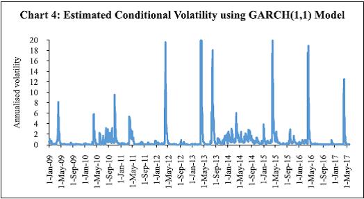
(May 2011) | Revised Liquidity Management Framework
(September 2014) | Modified Liquidity Framework
(April 2016) | • Repo rate - Single policy rate. • WACR is the operating target. • Corridor of +/- 100 bps around the repo rate • Full accommodation of liquidity demand at the fixed repo rate, albeit with an indicative comfort zone of +/-1 per cent of NDTL of the banking system. • Transmission of the changes in repo rate through the WACR to the term-structure of interest rates. | • Access to assured liquidity of about 1 per cent of Net Demand and Time Liability (NDTL) on an average • More frequent auctions of 14-day term repos during a fortnight (every Tuesday and Friday of a week). • Introduction of variable rate fine-tuning repo/ reverse repo auctions. | • The corridor around the repo rate narrowed from +/- 100 bps to +/- 50 bps. • Commitment to progressively lower the ex ante system level liquidity deficit to a position closer to neutrality in the medium-term. • Reducing the minimum daily maintenance of the Cash Reserve Ratio (CRR) from 95 per cent of the requirement to 90 per cent. | The operating framework, also termed as liquidity management framework, sub-serves the monetary policy framework in the sense that once the MPC announces the policy repo rate, based on its assessment of the macro-financial outlook for the economy, liquidity operations are conducted to keep the WACR (the operating target) close to the repo rate every day. The WACR emerges from the inter-bank unsecured segment of the overnight money market, and therefore best reflects the system-wide liquidity mismatch every day. Anticipating this liquidity mismatch through forecasting, and conducting liquidity injection/absorption operations to square the mismatch on a daily basis, hold the key to keeping the WACR close to the policy rate. The Liquidity Adjustment Facility (LAF) has a corridor around the policy repo rate with a Marginal Standing Facility (MSF) as its ceiling. This allows market participants to access central bank liquidity, at the end of the day, at a rate set currently at 25 basis points above the policy rate. Also, it allows a fixed rate overnight reverse repo window as the floor that allows market participants to place surplus liquidity at the end of the day with the RBI at a rate set at 25 basis points below the policy rate. Thus, the corridor restricts the extent of deviation of the WACR from the repo rate to (+/-) 25 bps. But proactive liquidity operations of the RBI aim at minimising recourse to either the ceiling or the floor of the corridor by the banks, which in turn contributes to finer alignment of the WACR to the repo rate. The LAF corridor was narrowed from +/-100 bps to +/-50 bps in April 2016, driven by the marksmanship of RBI’s liquidity operations in keeping the WACR close to the repo rate. The corridor was narrowed further to +/-25 bps in April 2017, in response to one-sided liquidity conditions post-demonetisation which imparted a sustained soft bias to the WACR relative to the repo rate (as discussed in greater detail later). The framework for dealing with frictional liquidity mismatch (Pillar I) and durable liquidity requirements of the economy (Pillar II) is set out in the Report of the Expert Committee to Revise and Strengthen the Monetary Policy Framework in India (RBI, 2014). The LAF deficit/surplus is the key indicator of net ‘liquidity’ demand of the banking system and of the economy as a whole on any single day, even though the magnitude of LAF deficit/surplus at any point of time need not be a reflection of the ‘liquidity conditions (i.e., tight/comfortable/easy)’ in the system. This is because of full accommodation of liquidity mismatch by the RBI that prevents both tightening of WACR during LAF deficits and its softening during LAF surpluses. The demand for funding liquidity of all non-banking sectors (households, corporates, and non-banking financial entities) in the economy, on every single day, needs to be met by the banking system. It can deal with this mismatch because of its exclusive access to the RBI’s LAF. Market liquidity (i.e., the ease with which any financial asset could be liquidated – sold or repoed – by an economic agent without altering its price), funding liquidity (i.e., ability of a bank to meet calls on liquidity from any of its customers), and central bank liquidity, are intertwined in a loop. Any market/funding liquidity pressure eventually gets manifested as LAF deficit/ surplus, because of full accommodation by the RBI. The banking system’s net demand for liquidity is effectively a reflection of the demand of the entire economy (i.e., non-banks and banks taken together). Liquidity transformation undertaken by banks – creating long-term assets based on liquid liabilities, or borrowing short to lend long – is necessary to harness the contribution of bank financing to growth and economic development. For banks, even while meeting the funding needs of the rest of the economy, their own access to funding liquidity (particularly from the money market, both collateralised and uncollateralised), market liquidity (that allows the use of liquid assets in their portfolio to raise funds when needed), and central bank liquidity, becomes critical. On a net basis, in India, the LAF position reflects the impact of all autonomous drivers of liquidity conditions (such as currency demand of households, liquidity impact of forex market interventions of the RBI, and changes in government’s cash balances maintained with the RBI) as well as non-LAF discretionary liquidity management operations [such as the Open Market Operations (OMOs), use of Market Stabilisation Scheme (MSS) securities/cash management bills (CMBs), and changes in the CRR]. Non-LAF operations minimise the pressure on LAF and also help meet the durable liquidity needs of a growing economy. The objective of a stable WACR could be achieved in India only after several years of reforms of the operating framework. As a brief background, the Committee on Banking Sector Reforms (Narasimham Committee II) first recommended the introduction of a liquidity adjustment facility (LAF) in 1998. Work towards transition to a full-fledged LAF started in June 2000 but, till 2003-04, the RBI’s market operations were dominated by outright purchase/sale of government securities. After the transition to LAF, the volatility in monthly average call rates, which used to move between a wide range of 5 to 35 per cent during 1990-98, declined significantly to a range of 5 to 10 per cent during the subsequent period (Mohan, 2006) (Chart 1). Repo and reverse repo rates operated as the ceiling and floor of the corridor, whose width changed several times in a year between 150 and 300 bps, up to the global financial crisis (GFC). 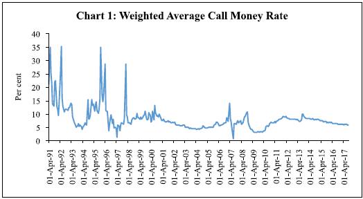 Three major exceptional periods since the GFC have tested liquidity management operations of the RBI. First, the post-GFC liquidity scare, when the RBI made available actual/potential liquidity of as high as 10 per cent of Gross Domestic Product (GDP). It did this through different instruments, such as cut in CRR, redemption/buyback of MSS securities, opening liquidity windows for Non-Banking Financial Companies (NBFCs), mutual funds and housing finance companies (through banks), besides the normal LAF and OMOs (Mohanty, 2009). Sudden spikes followed by significant easing of the WACR during this period reflected the initial scare-related scramble for liquidity, and the subsequent return of calm in the money market after the 425 bps cumulative cut1 in the policy rate and ample liquidity conditions created by the RBI. Two distinct aspects of liquidity operations of the RBI standout during this period: liquidity to non-banks, such as mutual funds, NBFCs and housing finance companies was provided only through banks; and, there was no dilution of collateral standards for allowing access to liquidity. Second, after the taper tantrum in mid-2013, the RBI used a monetary defence of the exchange rate by tightening liquidity conditions significantly and raising the effective money market rates by 300 bps (Pattanaik and Kavediya, 2015). Tighter daily average CRR maintenance norm (at 99 per cent) and caps on access to liquidity from the RBI (i.e., no full accommodation of liquidity demand) tightened the WACR, which started to ease when exceptional monetary measures were phased out (Chart 2). Third, the glut of surplus liquidity created after demonetisation in November 2016 prompted the RBI to use exceptional unremunerated incremental CRR of 100 per cent, temporarily, for one fortnight (RBI, 2017b). The liquidity overhang continued for more than a year after demonetisation, and persistent surplus conditions imparted a softening bias to the WACR through the year. The post-demonetisation behaviour of the WACR is particularly striking from the standpoint of empirical implications for monetary policy transmission. Because of the sustained soft bias, the spread between WACR and the policy repo rate remained persistently negative, averaging about 30 bps in March 2017 (after rising over successive months). And as a result of this the LAF corridor was narrowed from +/- 50 bps to +/-25 bps in April 2017. Since then, the average spread has declined to about (-) 13 bps2 (Chart 3). Unlike the volatile daily spread, however, conditional volatility of WACR generally remained very low, but for the usual year-end effects associated with balance sheet adjustment by banks (Chart 4). The available empirical research on different aspects of the operating framework of monetary policy in India provide useful insights for the empirical approach adopted in the next section. Spread (defined as the bid-ask difference in the inter-bank call money market, rather than the difference between the WACR and the repo rate) was found to be influenced by liquidity conditions (i.e., size of LAF deficit/surplus) and uncertainty (i.e., conditional variance of the cumulative average of reserve maintenance ratio during the fortnightly CRR maintenance period). The impact of uncertainty on the spread, however, has diminished significantly in recent years, reflecting the role of operating framework reforms in reducing uncertainty about liquidity conditions (Kumar et al., 2017). A different measure of uncertainty used in another study, i.e., conditional volatility of the WACR, was also found to be imparting an upside to the spread (defined also as the bid-ask difference, but between Mumbai Inter-Bank Bid Rate and Mumbai Inter-Bank Offer Rate) (Ghosh and Bhattacharyya, 2009). From the standpoint of assessment of the effective functioning of the operating framework, what may be more important is to study spread in terms of deviation of the WACR from the policy repo rate. Both these rates, as one would expect, are co-integrated, and the error-correction term suggests that deviations of the WACR from the repo rate are short-lived (Patra et al., 2016). Volatility in WACR was found to have a statistically significant and positive impact on the 90-day Treasury Bills rate. But after excluding the GFC period from the sample, the statistical significance of the impact disappeared. Unlike these studies, the emphasis of this paper is on the entire term structure (across the yield curve) and also bank-lending rates which are critical to influence consumption and investment decisions and, therefore, to an assessment of monetary policy transmission. 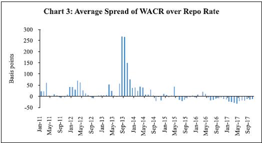
 Section III
Data, Methodology and Empirical Findings This paper uses daily data for the period January 2009 to May 2017, which covers all the three major liquidity shocks mentioned in the previous section. It also starts before the crucial May 2011 reform of the operating framework. The interest rates across the term-structure considered comprise yields on three-month, six-month, nine-month and twelve-month treasury bills and two-year and ten-year government securities. Stationarity of these interest rates is examined using the Augmented Dickey-Fuller (ADF), the Phillips-Perron and the Kwiatkowski–Phillips–Schmidt–Shin (KPSS) tests, which suggest that all of them are stationary in their first difference (Table 2). Accordingly, variables are used in their first difference form in subsequent analysis. The summary statistics of WACR and daily change in WACR are presented in Table 3. On an average, daily change in WACR is minimal over the sample period. The variance of daily WACR is 3.20 while the variance of daily ΔWACR is 0.08. The negative skewness coefficient indicates that the distribution of daily changes in WACR is negatively skewed. The large value of kurtosis reflects the thick tails of the distribution. The Jarque-Bera statistics, besides skewness and kurtosis, indicate non-normal distribution of daily changes in WACR. The residuals obtained by modelling the first difference of WACR, using the Ordinary Least Squares (OLS) method3, suggested that large residuals tend to be followed by large residuals and small residuals tend to be followed by small residuals, pointing to the presence of volatility clustering (Chart 5). While the Breusch-Pagan-Godfrey test suggested the presence of heteroskedasticity, the Ljung-Box test indicated the presence of serial autocorrelation in residuals. All these pre-tests suggested the GARCH model as appropriate for modelling volatility in the operating target. | Table 2: Unit Root Test Results | | | ADF test | Phillips-Perron Test | KPSS Test* | | None | p-val | Inter- cept | p-val | Intercept and trend | p-val | None | p-val | Inter- cept | p-val | Inter- cept and trend | p-val | Inter- cept | Inter- cept and trend | | Level | | | | | | | | | | | | | | | | WACR | -0.42 | 0.53 | -1.94 | 0.31 | -1.92 | 0.64 | -0.32 | 0.57 | -3.09 | 0.03 | -3.45 | 0.05 | 2.22 | 1.33 | | tb3m | -0.09 | 0.65 | -1.57 | 0.50 | -1.21 | 0.91 | -0.10 | 0.65 | -1.56 | 0.50 | -1.20 | 0.91 | 2.24 | 1.32 | | tb6m | 0.01 | 0.69 | -1.57 | 0.50 | -1.12 | 0.92 | -0.01 | 0.68 | -1.58 | 0.49 | -1.13 | 0.92 | 2.21 | 1.32 | | tb9m | 0.05 | 0.70 | -1.59 | 0.49 | -1.10 | 0.93 | 0.04 | 0.70 | -1.58 | 0.49 | -1.10 | 0.93 | 2.19 | 1.33 | | tb12m | 0.17 | 0.73 | -1.49 | 0.54 | -0.87 | 0.96 | 0.11 | 0.72 | -1.59 | 0.49 | -1.07 | 0.93 | 2.16 | 1.33 | | gsec2yr | 0.20 | 0.74 | -2.20 | 0.21 | -1.62 | 0.78 | 0.20 | 0.74 | -2.21 | 0.20 | -1.67 | 0.76 | 1.93 | 1.32 | | gsec10yr | 0.34 | 0.78 | -3.23 | 0.02 | -3.07 | 0.12 | 0.24 | 0.76 | -3.40 | 0.01 | -3.28 | 0.07 | 1.10 | 1.09 | | First Difference | | | | | | | | | | | | | | | | dWACR | -25.22 | 0.00 | | | | | -75.31 | 0.00 | | | | | 0.19 | 0.08 | | dtb3m | -14.48 | 0.00 | | | | | -51.38 | 0.00 | | | | | 0.22 | 0.06 | | dtb6m | -15.29 | 0.00 | | | | | -51.31 | 0.00 | | | | | 0.27 | 0.06 | | dtb9m | -15.01 | 0.00 | | | | | -49.86 | 0.00 | | | | | 0.29 | 0.06 | | dtb12m | -33.70 | 0.00 | | | | | -63.11 | 0.00 | | | | | 0.35 | 0.06 | | dgsec2yr | -13.22 | 0.00 | | | | | -65.51 | 0.00 | | | | | 0.39 | 0.02 | | dgsec10yr | -35.54 | 0.00 | | | | | -44.61 | 0.00 | | | | | 0.59 | 0.05 | | *: Cut-off value of KPSS test with ‘intercept’ and ‘intercept and trend’ at 1 per cent level of significance are 0.74 and 0.22, respectively. |
| Table 3: Summary Statistics of WACR and Daily Change in WACR | | | WACR | ∆WACR | | Mean | 6.78 | 0.00034 | | Variance | 3.20 | 0.0846 | | Skewness | -0.64 | -0.5540 | | Kurtosis | 2.89 | 99.45 | | Jarque-Bera Statistic | 149.8* | 850880* | | *: Significant at 1 per cent level. | Estimation of Volatility of WACR The WACR, as in the case of many other financial market variables, displays periods of volatility and periods of calm. Further, while modelling the volatility of financial variables, it is often found in the literature that the sum of the estimated parameters of standard GARCH (1, 1) are close to unity, which is an indication of strong volatility persistence. Taking into account the persistence of volatility in WACR, the integrated GARCH (IGRACH) model proposed by Engle and Bollerslev (1986) is used to model volatility. Specifically, the following IGARCH (1, 1) model is used: Mean equation: Variance equation: Diagnostic tests of residuals suggest that the model is specified correctly to capture the volatility in WACR. The Ljung-Box Q-statistic and ARCH-LM statistics indicate that the model is free from autocorrelation. Also, the Ljung- Box Q-statistic at 20th lag of the squared standardised residuals was at 0.1844 (with p-value close to 1), indicating that the standardised squared residuals are serially uncorrelated. The WACR is found to be negatively autocorrelated. A one percentage point increase in the policy repo rate leads to 0.8 percentage point rise in WACR in the same time period. Thereafter, remaining gap between WACR and repo rate is adjusted through the Error Correction Term (ECT) at the rate of 0.05 percentage point per day. The impact of liquidity conditions on changes in WACR is estimated to be positive and significant. This may be interpreted as any pressure on WACR is essentially an indication of higher demand for liquidity, which is fully accommodated through the central bank's liquidity windows, leading to higher net LAF injection. Calendar effects are statistically significant. The positive and significant effect of taper tantrum is in line with the intuition, since during this phase the RBI restricted access to central bank liquidity and made the ceiling of the LAF corridor as the effective policy rate. In the variance equation, both ARCH and GARCH terms are significant. | Table 4: Conditional Volatility of WACR using IGARCH(1,1)* Dependent Variable: ΔWACR | | | Coefficient | p-value | | Coefficient | p-value | | Mean Equation | Volatility Equation* | | Constant | -0.001 | 0.19 | RESID(-1)^2 | 0.244 | 0.00 | | ∑∆WACR | -0.24 | 0.00 | GARCH(-1)^2 | 0.756 | 0.00 | | ∑∆Repo Rate | 0.80 | 0.03 | DUM_MARCH | 0.342 | 0.00 | | Net Liquidity | 0.002 | 0.00 | | | | | ECT | -0.050 | 0.00 | | | | | Dum_March | 1.186 | 0.00 | | | | | Dum_April | -1.413 | 0.00 | | | | | Dum_Taper | 0.136 | 0.00 | | | | | D3 | 0.039 | 0.00 | | | | | D10 | 0.004 | 0.09 | | | | | D11 | -0.010 | 0.00 | | | | | D13 | -0.004 | 0.04 | | | | | T-DIST. DOF | 3.244 | 0.000 | | | | | Q(10) | 12.446 | 0.256 | | | | | Q(20) | 23.144 | 0.282 | | | | | ARCH LM (5) | 0.430 | 0.828 | | | | | *: The dummy representing the impact of demonetisation is insignificant in both mean and variance equations, while the dummy relating to the taper tantrum event is insignificant in the variance equation. | Transmission of Volatility The estimated conditional volatility of daily changes in WACR is used as a determinant of the term structure of interest rates in respective mean and variance equations, while retaining the same structural specifications as in equations 1 and 2. Mean equation Variance equation Impact of Volatility in WACR on Banks’ Lending Rates Transmission of a monetary policy-easing action to retail interest rates could be impeded if an inter-bank rate volatility shock occurs at the same time when the policy rate is lowered (Bouvatier and Chahad, 2014). On the contrary, the impact of a restrictive monetary policy can be amplified in times of high inter-bank rate volatility. Ritz (2012) argued that a rise in funding uncertainty dampens interest rate pass-through. In a cross-country study, however, Raunig and Scharler (2009) found limited impact of transmission of volatility in money market rates to volatility in retail interest rates. | Table 5: Volatility Transmission from the Overnight Segment to Interest Rate Term-structure | Dependent
Variable | DTB3M | DTB6M | DTB9M | DTB12M | DG-sec 2_yr | DG-sec 10_yr | | Coeff | P-val | Coeff | P-val | Coeff | P-val | Coeff | P-val | Coeff | P-val | Coeff | P-val | | Mean Equation | | | | | | | | | | | | | | Constant | 0.0011 | 0.02 | -0.0005 | 0.30 | 0.0003 | 0.48 | 0.0002 | 0.69 | -0.0002 | 0.00 | -0.0003 | 0.65 | | dep(-1) | -0.0468 | 0.00 | -0.0295 | 0.01 | -0.0532 | 0.00 | -0.0949 | 0.00 | -0.0873 | 0.00 | 0.0258 | 0.13 | | D_Repo | 0.1350 | 0.00 | 0.2077 | 0.00 | 0.2317 | 0.00 | 0.1586 | 0.00 | 0.0028 | 0.00 | 0.0401 | 0.00 | | Net Liquidity | -0.0001 | 0.69 | 0.0003 | 0.24 | 0.0002 | 0.49 | 0.0004 | 0.13 | 0.0002 | 0.00 | -0.0002 | 0.62 | | Dum_March | -0.0585 | 0.00 | -0.0512 | 0.00 | -0.0240 | 0.00 | -0.0215 | 0.00 | 0.0004 | 0.42 | -0.0206 | 0.00 | | Dum_Taper | 0.0146 | 0.37 | 0.0018 | 0.87 | 0.0191 | 0.17 | 0.0058 | 0.80 | -0.0198 | 0.69 | 0.0007 | 0.96 | | Dum_demonetisation | -0.0031 | 0.53 | -0.0055 | 0.10 | -0.0029 | 0.65 | 0.0005 | 0.93 | -0.0123 | 0.00 | -0.0050 | 0.48 | | Garch ON vol | -0.0052 | 0.37 | -0.0016 | 0.69 | -0.0039 | 0.39 | -0.0047 | 0.54 | 0.0000 | 0.98 | -0.0005 | 0.88 | | Variance Equation | | | | | | | | | | | | | | RESID(-1)^2 | 0.0339 | 0.00 | 0.0234 | 0.00 | 0.0591 | 0.00 | 0.1596 | 0.00 | 0.0265 | 0.00 | 0.0579 | 0.00 | | GARCH(-1) | 0.9661 | 0.00 | 0.9766 | 0.00 | 0.9409 | 0.00 | 0.8404 | 0.00 | 0.9735 | 0.00 | 0.9421 | 0.00 | | Garch ON vol | 0.0004 | 0.00 | 0.0002 | 0.00 | 0.0003 | 0.00 | 0.0014 | 0.00 | 0.0000 | 0.58 | 0.0002 | 0.00 | | DUM_MARCH | 0.0024 | 0.02 | 0.0005 | 0.41 | 0.0000 | 0.99 | -0.0008 | 0.00 | -0.0004 | 0.00 | -0.0007 | 0.00 | | Q(10) | 14.7 | 0.14 | 11.2 | 0.34 | 8.1 | 0.62 | 5.5 | 0.86 | 0.1 | 1.00 | 8.7 | 0.56 | | Q(20) | 21.0 | 0.39 | 13.6 | 0.85 | 10.4 | 0.96 | 7.7 | 0.99 | 1.1 | 1.00 | 13.1 | 0.87 | | ARCH LM (5) | 0.001 | 0.99 | 0.02 | 0.98 | 0.001 | 0.99 | 0.0 | 0.99 | 0.0 | 0.99 | 0.1 | 0.92 | | Note: Coefficients in bold font are statistically significant at 5 per cent or lower levels. | With a view to examining the impact of volatility in WACR on banks’ lending rates (rather than identifying all determinants of lending rates), quarterly data for a panel of fifty-eight banks (covering public, private and foreign banks) are used over the period June 2012 to June 2017, for which data on bank-wise weighted average lending and deposit interest rates are available. The following dynamic panel model is estimated: 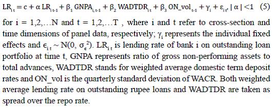 By construction, LRi t-1 depends on individual fixed effects, leading to the endogeneity problem. The OLS, or fixed effect models, generally provide biased estimates for small T and large number of cross-section N. Further, inclusion of lagged dependent variables gives rise to the problem of autocorrelation. To estimate the dynamic panel regression (5), with the panel having a larger number of banks relative to the time period, we use the difference GMM approach proposed by Arellano and Bond (1991). This approach controls for the unobserved individual bank-specific effects and also addresses the issue of endogeneity of explanatory variables. The first-difference of the panel data helps to remove the time-invariant fixed effects. The values (levels) of the lagged dependent variables work as valid instruments for the first-differenced variables, provided that the residuals are free from second-order serial correlation. For testing autocorrelation, Arellano-Bond test is used, while the validity of the instrument is tested using the Sargan test of over-identifying restrictions. Empirical findings suggest that lending rates of banks are positively autocorrelated with their past values. Also, volatility in overnight WACR has a positive and statistically significant impact on banks’ lending rate. A one percentage point increase in overnight volatility may lead to about 26 basis points increase in bank lending rates. The GNPA ratio, as expected, has a positive and statistically significant relationship with bank lending rates (Table 6). Table 6: Impact of Volatility in WACR on Lending Rates of Banks
Dependent Variable: Lending Rate (LR) | | | Coeff. | P-value | | Constant | 1.74 | 0.00 | | LR(-1) | 0.42 | 0.00 | | WADTDR | 0.80 | 0.00 | | GNPA | 0.09 | 0.06 | | ON_vol(-1) | 0.26 | 0.01 | | | Wald Chi-square | 184.3 | | | | (0.00) | | | AR(1) | -3.12 | | | | (0.00) | | | AR(2) | -0.09 | | | | (0.92) | | | Sargan stat. (2-step) | 55.35 | | | | (0.28) | Section IV
Conclusion The operating framework of monetary policy, which is about implementation of monetary policy on a day-to-day basis, strives to ensure the first leg of monetary policy transmission by aligning the overnight money market rates close to the policy rate. The combination of a LAF corridor that restricts intra-day volatility in overnight rates and proactive liquidity management by a central bank that limits the need for recourse to its liquidity at the upper/lower bounds of the corridor helps in keeping the overnight money market rates close to the policy rate. In the assessment of the role of an effective operating framework, however, besides the first leg of transmission, the scope for influencing the entire term structure of interest rates by minimising volatility in the overnight rates, and in the operating target in particular, has also gained prominence. Long-term rates, which matter to the real economy, essentially reflect the expected future path of short-term rates and a time-varying term premium as a compensation for uncertainty. Recognising the importance of expectations about the future path of short-term rates to effective monetary policy transmission, monetary policy frameworks have strived to become increasingly more predictable and transparent, with an emphasis on communication relating to the central bank’s assessment of the macroeconomic outlook as well as the likely policy reaction function. An operating framework of monetary policy that emphasises stability of the operating target can sub-serve the monetary policy framework better by limiting transmission of volatility from the operating target to the term premium, and, therefore, to the term structure of interest rates. In India, successive reforms in the operating framework have enabled finer alignment of the WACR – the operating target of monetary policy – to the policy repo rate. Nevertheless, WACR being a market-determined rate, its volatility has been non-zero, though modest. This paper examined whether volatility in WACR has had any statistically significant influence on the term structure of interest rates. Conditional volatility in daily change in WACR – extracted from an IGARCH (1,1) model – does not exert any statistically significant influence on daily change in other interest rates, namely nominal yields on government papers of three-month, six-month, nine-month, twelve-month, two-year and ten-year maturities. Volatility in other interest rates, however, is found to have been influenced by volatility in daily change in WACR, particularly up to a one-year tenor. The magnitude of the impact is estimated to be low – a one percentage point increase in conditional volatility of daily change in WACR leading to higher volatility in other interest rates by 0.02 to 0.14 basis points. To examine the impact of volatility in WACR on bank lending rates, which is more important to the credit market and therefore aggregate demand, a panel regression approach was adopted covering quarterly data from June 2012 to June 2017 for fifty-eight banks and the model was estimated using difference GMM. In the panel regressions, volatility is captured as actual observed volatility in WACR in terms of quarterly standard deviations, as against the conditional volatility of daily change in WACR used in other equations to study the impact on market interest rates. A one percentage point increase in WACR volatility is estimated to cause about 26 basis points increase in bank lending rates. The impact assessment on the lending rates suggests the need for reducing the volatility in WACR even further through proactive liquidity management.
References Alper, E., C. Morales, and F. Yang (2016), “Monetary Policy Implementation and Volatility Transmission along the Yield Curve: The Case of Kenya”, IMF Working Paper No. 16/120, 20 June. Available at:
https://www.imf.org/en/Publications/WP/Issues/2016/12/31/Monetary-Policy-Implementation-and-Volatility-Transmission-along-the-Yield-Curve-The-Case-of-43995. Arellano, M. and S. Bond. (1991), “Some Tests of Specification for Panel Data: Monte Carlo Evidence and an Application to Employment Equations”, The Review of Economic Studies, 58, pp. 277–97. Ayuso, J., A. Haldane and F. Restoy (1997), “Volatility Transmission along the Money Market Yield Curve”, Review of World Economics, 133(1), pp. 56–75. Bouvatier, V. and Chahad, M. (2014), “Interest Rate Pass-through and Interbank Rate Volatility Shocks: A DSGE Perspective”, February. Available at:
http://www.touteconomie.org/afse2014/index.php/meeting2014/lyon/paper/viewFile/439/233. Brock, Philip L. and Liliana Rojas Suarez (2000), “Understanding the Behavior of Bank Spreads in Latin America”, Journal of Development Economics, 63, pp. 113–34. Carpenter, Seth B., Selva Demiralp and Zeynep Senyuz (2016), “Volatility in the Federal Funds Market and Money Market Spreads during the Financial Crisis”, Journal of Financial Stability, 25, pp. 225–33. Chiu, Ching-Wai, Richard D.F. Harris, Evarist Stoja, and Michael Chin (2016), “Financial Market Volatility, Macroeconomic Fundamentals and Investor Sentiment”, Bank of England Working Paper No. 608, August 23. Cohen, Benjamin (1999), “Monetary Policy Procedures and Volatility Transmission along the Yield Curve,” CGFS Papers, Bank for International Settlements (ed.), Market Liquidity: Research Findings and Selected Policy Implications, 11, pp. 1–22. Colarossi, Silvio and Andrea Zaghini (2009), “Gradualism, Transparency and Improved Operational Framework: A Look at Overnight Volatility Transmission’, International Finance, 12(2), pp. 151–70. Eickmeier, Sandra, Norbert Metiu and Esteban Prieto (2017), “Monetary Policy Effectiveness in Times of Financial Market Volatility”, Deutsche Bundebank, Research Brief 11th edn., March. Available at:
http://www.bundesbank.de/Redaktion/EN/Kurzmeldungen/Research_brief/2017_11_monetary_policy_ financial_market.html. Engle, Robert and Andrew Patton (2001), “What Good is a Volatility Model?”, Quantitative Finance, 1, pp. 237–45. Engle, Robert and Bollerslev, T. (1986), “Modeling the Persistence of Conditional Variances”, Econometric Reviews, 5, pp. 1–50. Gaston Gelos, R. (2006), “Banking Spreads in Latin America”, IMF Working Paper 06/44, February. Ghosh, Saurabh and Indranil Bhattacharyya (2009), “Spread, Volatility and Monetary Policy: Empirical Evidences from the Indian Overnight Money Market”, Macroeconomics and Finance in Emerging Market Economies, 2(2), pp. 257–77. Kumar, Sunil, Anand Prakash and Krishna Kushwaha (2017), “What Explains Call Money Rate Spread in India?”, RBI Working Paper 7/2017, April. Mohan, Rakesh (2006), “Coping With Liquidity Management in India: A Practitioner’s View”, Address at the 8th Annual Conference on Money and Finance in the Indian Economy at Indira Gandhi Institute of Development Research (IGIDR), March 27, 2006. Mohanty, Deepak (2009), “Global Financial Crisis and Monetary Policy Response in India”, RBI Bulletin, December. Osborne, Matthew (2016), “Monetary Policy and Volatility in the Sterling Money Market”, Bank of England Working Paper No. 588, April. Patra, Michael Debabrata, Muneesh Kapur, Rajesh Kavediya and S.M. Lokare (2016), “Liquidity Management and Monetary Policy: From Corridor Play to Marksmanship”, in Kenneth M. Kletzer and Chetan Ghate (eds.), Monetary Policy in India. Pattanaik, Sitikantha and Rajesh Kavediya (2015), “Preconditions to the Success of an Interest Rate Defence of the Exchange Rate”, Prajnan, December. Raunig, B. and J. Scharler (2009), “Money Market Uncertainty and Retail Interest Rate Fluctuations: A Cross-country Comparison”, German Economic Review, 10(2), pp. 176–92. Reserve Bank of India (RBI) (2014), Report of the Expert Committee to Revise and Strengthen the Monetary Policy Framework (Chairman: Dr. Urjit R Patel). Available at:
https://rbidocs.rbi.org.in/rdocs/PublicationReport/Pdfs/ECOMRF210114_F.pdf. — (2017a), Report of the Internal Study Group to Review the Working of the Marginal Cost of Funds Based Lending Rate System (Chairman: Dr. Janak Raj). Available at:
https://rbi.org.in/scripts/PublicationReportDetails.aspx?ID=878. — (2017b), “Macroeconomic Impact of Demonetisation - A Preliminary Assessment”, RBI, March 10, 2017. Available at:
https://rbidocs.rbi.org.in/rdocs/Publications/PDFs/MID10031760E85BDAFEFD497193995BB1B6DBE602.PDF. Ritz, R. A. (2012), “How do banks respond to increased funding uncertainty?” Cambridge Working Papers in Economics CWPE 1213, Faculty of Economics, University of Cambridge. Stein, Jeremy C. and Adi Sunderam (2017), “The Fed, the Bond Market, and Gradualism in Monetary Policy”, April. Available at:
http://scholar.harvard.edu/files/stein/files/gradualism_20170428_002.pdf.
|