Indrajit Roy, Anirban Sanyal, Aloke Kumar Ghosh^*

This paper attempts to nowcast quarterly real non-agricultural Gross Value Added (GVA) growth for India using a dynamic factor model (DFM), following two different approaches. Multi-level variable selection using turning-point analysis and elastic-net framework has been adopted to overcome the over-fitting problem while selecting of variables. The paper finds significant improvement in forecast accuracy of one-quarter ahead forecast using nowcasting framework as compared with the naïve models. The two-factor model is found to be the most precise when compared with other higher-order factor models and naïve models. The forecast performance improves marginally when stochastic volatility is introduced in the model.

JEL Classification : C51, C52, C53, C32, C38, E50, E17

Keywords : Nowcasting, Cross-correlation, Business cycle, LARS-EN, Dynamic factor model, Kalman filter, Principal component, Cross-section

Introduction

Central banks track various macroeconomic indicators for forward-looking assessment of the state of an economy. Gross Domestic Product (GDP) is an important component for policy analysis. However, data relating to GDP are released with a lag and the release calendar is often asynchronous with the monetary policy calendar. In the absence of any real-time information on GDP, ‘central banks’ adopt different strategies to deal with the data gaps. Forecasting is one option which can provide forward-looking guidance on economic growth. Model-based forecasting is often criticised for limited information content, while incorporating a larger information set brings in the problem of dimensionality. The other approach, namely ‘multiple indicator’ approach, is governed by tracking high-frequency data of economic indicators. The challenge arises when different indicators depict diverging scenarios about the state of the economy. In such a situation, summarising the information content from a larger information set and incorporating only the relevant information in the forecasting model provides a viable solution. Such an approach, also called nowcasting, gained popularity among forecasters in the aftermath of the global financial crisis of 2007.

The background of nowcasting goes back to the introduction of bridge models, which were formulated to bridge the gap between target series using available indicators (Bessec, 2013). However, the ‘curse of dimensionality’ restricted the use of a large information set. Stock and Watson (1999, 2002) introduced the first static and dynamic factor model for incorporating a larger information set using factors. The nowcasting framework builds upon the dynamic factor model (DFM) in a mixed-frequency setup in such a manner that the factors are updated based on the latest available information. In this context, the nowcasting framework suggested by Giannone et al. (2008) used around 200 high-frequency economic indicators with a varying data release calendar for nowcasting the US GDP using DFM. Later on, other central banks started incorporating similar nowcasting frameworks for short-term forecasting (Angelini et al., 2011; Altissimo et al., 2001, 2007; Schumacher, 2007, 2010; D’Agostino et al., 2008; Marcellino et al., 2013). The emergence of nowcasting and its wide adaptability point towards its growing popularity among economic forecasters and policymakers. Over fifty-four different research papers on short-term forecasting have been published in different top-ranked international journals between 2014 and 2016, which highlights the sustained interest in the methodologies for improving short-term forecasting.

While nowcasting has been adopted across advanced economies in the aftermath of the financial crisis of 2007, the emerging market economies (EMEs), which face comparatively more severe data release lags and revisions, started exploring the potential of nowcasting only in recent times. In India, the Central Statistics Office (CSO) releases quarterly GDP/ GVA data after a lag of about 60 days. For instance, GDP/GVA estimates for Q3: 2016-17 were released on February 29, 2017 i.e., after a lag of about two months. Hence, any assessment of growth in the current quarter has to rely on the information available on high-frequency indicators. Nowcasting can help estimating GVA using the latest available information on such economic indicators, before the release of first advance estimate by the CSO. It can also incorporate the periodic data revisions for updating the short-term forecast of GVA.

In this paper, an attempt has been made to apply two main available nowcasting approaches to Indian data. The short-term forecasts generated from these nowcasting approaches have been validated against the available short-term forecasting models (also called naïve models) using an expanding-window approach. The variable selection for factor model has been carried out by applying a multi-level approach to turning point analysis mimicking business cycle approach. The paper finds significant improvement in short-term forecast precision using nowcasting models as compared to naïve models. The rest of the paper is organised as follows. Section II presents a brief literature review on the different approaches to use DFM in nowcasting. Section III illustrates the methodology along with a separate discussion on selection of variables. Details of data used are presented in Section IV, followed by the empirical findings in Section V. Section VI concludes with a few remarks on the proposed approach for nowcasting Indian GDP/GVA.

Section II
Literature Review

Dynamic factor models emerged as an effective mechanism for reducing dimensionality in the forecasting domain. Unlike the first and second generation DFM, the third generation deals with the time invariant correlation structure, using a larger data set in state space framework (Stock, 2010). In this approach, a principal component analysis (PCA) is used to derive the initial estimates of the factors and subsequently the factors are updated based on the latest available observations of the constituent economic indicators in a state-space framework. The use of factor models for nowcasting in a mixed frequency setup was formally introduced by Giannone et al. (2008), where the nowcasting model was developed using monthly data on a large set of macroeconomic and other indicators. The use of DFM for nowcasting GDP was first used in 2005 by the Board of Governors of the US Federal Reserve. Angelini et al. (2011) introduced a similar framework for the European Central Bank (ECB). The research work of Altissimo et al. (2011), Schumacher (2007 and 2010), and D’Agostino et al. (2008) in the related area helped to introduce this framework in Banca d’Italia, Bundesbank and Central Bank of Ireland, respectively. Barhoumi et al. (2010) compared the forecast performance of dynamic factor models with other quarterly models (AR, VAR and bridge equations) for select European countries and they observed significant improvement in forecasting performance in case of dynamic factor models that used monthly data. As regards variable selection, soft data which are primarily obtained through different surveys and available in a timely manner are used in DFM. However, the forecasting precision using such soft indicators is often found to be weaker than that using hard data (Banbura and Runstler, 2011). With this background, Giannone et al. (2008) used both hard and soft indicators for nowcasting GDP. Camacho et al. (2010) used a similar approach for developing the Euro-STIN. Euro-STIN represents a model that combines short-run economic indicators along with GDP revisions for increasing the precision of short-term forecasts of GDP in the Euro area. Their approach incorporated the Kalman filter model of Mariano and Murasawa (2003) to deal with mixed frequency on top of the ‘strict DFM’ framework of Stock and Watson (1991). The information content of GDP data revisions was previously used by Evans (2005) and Coenen et al. (2005). However, the incorporation of revision history along with soft and hard data was first introduced in Euro- STIN. The framework used in Euro-STIN was later extended by Marcellino et al. (2013) for nowcasting the Euro area GDP. The novelty of this framework was that stochastic volatility was introduced using the time-varying variance parameter. The model was estimated using multi-move Gibbs sampling approach as suggested by Carter and Kohn (1995). While nowcasting GDP of Germany, Girardi et al. (2016) observed improvement in short-term forecast performance using the partial least square approach for deriving the factor estimate. Lamprou (2016) and Feldkircher (2016), however, observed that DFM using bridge model had better forecast precision compared to time series models. The forecast performance of these models, nevertheless, was found to be changing over time and that suggested for a continuous review of the modelling framework to improve forecast performance (Feldkircher, 2016).

Section III
Framework

India’s GVA data are released by the CSO at a quarterly frequency with a lag of about 60 days. The quarterly growth rate of GVA (Y_t^q) for any current quarter, therefore, has to be forecast based on monthly available data. In this process, two different situations generally arise – firstly the data vintages change after the release of data and accordingly, the information base of nowcasting changes; secondly, as the new data become available, the old data get revised and the dynamics change. Also, the data release calendars of different indicators in any month vary across months and thus at any point of time, the chance of getting ’Jagged Heads’ or ’unbalanced panel’ is significantly high. This paper considers a dynamic factor model for nowcasting GDP using approaches suggested by Giannone et al. (2008) and Marcellino et al. (2013).

Framework used by Giannone

Giannone et al. (2008) used a dynamic factor model encompassing a large set of indicators. As the number of indicators increases, the number of unknown parameters also increases, and the curse of dimensionality crops up which limits degrees of freedom for residual estimates. The factor models are used for overcoming the dimensionality problem while capturing the information to a major extent.

Since the data release calendar of different variables within the information set {X_t} differs, the chance of getting an unbalanced panel cannot be ruled out. For that, we assume that:

which indicates the incremental information content in the latest available vintage over the previous data release.

Framework used by Marcellino

Marcellino et al. (2013) assumed that the quarterly estimate of GVA is assumed to be a geometric average of monthly unobserved GVA figures. Such assumption is viable in case the month on month changes in GVA are expected to be minimal. Under this assumption,

Following Kim and Nelson (1999), the model was estimated using the multi move Gibbs Sampling approach with Metropolis Hastings algorithm for selecting the draws.

Naïve Models

The forecast performance of the nowcasting models has been analysed using the rolling forecast approach with expansionary window size. The benchmark models considered in this paper fall under time series and structural models. A list of naïve models used in this paper is given below:

The lag selection of VAR models has been decided using SIC criteria. Further, the time varying models of VAR have been framed in line with Primeceri (2005) and estimated using multi move Gibbs Sampling following Cater and Cohn (1994). In-sample residual diagnostics and test of convergence¹ have been validated for goodness of fit and stability.

Section IV
Selection of Variables

The success of a dynamic factor models lies in extracting factors from a pool of economic variables which contain information on the target variable. Thus, the information content of each variable should be cross checked before selecting a final pool. Stock and Watson (1999 and 2002) advocated the use of very large information sets, which have also been considered in a majority of the papers that use DFM. Giannone et al. (2008) incorporated 200 odd economic indicators for nowcasting US GDP growth. However, a different stance was adopted by Bai and Ng (2008) and Boivin and Ng (2006), who suggested the use of a relatively smaller set of variables to start with. Following that methodology, Angelini et al. (2011) and Camacho et al. (2010) used a smaller set of variables (also called core variables) and then incrementally included more variables one by one, based on improvement in forecast performance.

One most commonly accepted way to check the nature of dependence among the variables is the cross-correlation test which not only provides the significance of cross-correlation at various lags but also suggests the nature of dependence using the sign of correlation. In this context, the variables showing significant cross correlation at lag = 0 and having appropriate signs comprise the first pool of variables. However, while high cross-correlation affirms a co-movement among the series, it does not address one of the major aspects of a business cycle, that is switching of processes between which is identified as the most critical property of any business cycle indicator by Burns and Mitchell (1946). In view of this, Lahiri and Yao (2006) used turning point analysis by applying Bry-Boschan (1971) algorithm. The turning point analysis of the target variable and other economic indicators provide sufficient insight about the different phases of business cycle movement observable in each series. Though Lahiri and Yao (2006) proposed statistical coherence tests for identifying regime changes, the scrutiny of turning point analysis of any business cycle indicator requires sufficiently large number of observations, which is not suitable for our study due to the limitation of adequate data points. So, we rely on visual inspection of regime switches in the target variable and the explanatory variables. Comparing the regimes of target series, any variable (or regressor) having recession and boom regimes during different periods would be suspected for the fact that the concerned regressor would not be able to predict the turnaround points of the target variable efficiently. Hence, the cross-correlation test along with regime switching behaviour would provide sufficient screening of regressors for nowcasting. Adding up variables based on the above criteria could be one solution to define a larger pool of variables.

On the contrary, as identified by Boivin and Ng (2006), adding more and more variables into dataset may not result in improvement of forecasting performance, as some of the variables may have influences from other variables which do not impact the target variable. Also, if the idiosyncratic components are large and correlated with each other, adding further variables may not result in better accuracy in forecasting. Thus, pre-selection of variables poses a crucial challenge to forecasting. Marie (2013) used elastic net framework using least angle regression - Elasticnet (LARS-EN) algorithm for selecting the regressor. LARS-EN algorithm typically uses sequential backward selection of variables using ARDL model for checking the explanatory power of regressors and penalising L1 and L2 norm of regression coefficients.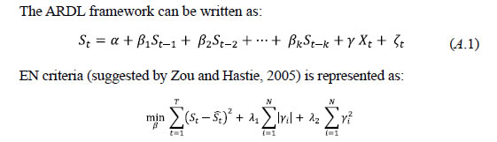

where λ₁ and λ₂ are the penalty parameters of L¹ and L² norms of regression coefficients. Basically, EN criteria is a combination of LASSO and Ridge regression which Zoe and Hastie (2005) suggested as more efficient than LASSO and Ridge. So we resort to LARS-EN algorithm for the final selection of pooled regressor.

Section V
Data Used

In this paper, GVA at basic price has been considered for nowcasting. As a supply-side measure, GVA at basic prices (real) comprises three major sectors namely agriculture (around 14-15 per cent), industry (around 22-23 per cent) and services (around 57-62 per cent). Among these three sectors, agriculture growth remains highly seasonal in nature and depends upon exogenous variables like rainfall, reservoir status and sowing pattern, the information on some of which are not available at higher frequency. Hence, GVA excluding the agriculture sector (also called non-agriculture GVA) has been considered as the target variable for the nowcasting exercise in this paper. GVA data are available from Q1: 2011-12, only after the latest rebasing exercise carried out by the CSO. The back series of GVA at basic prices has been constructed using a bottom-up approach. Using this approach, the linking factor has been estimated separately for agriculture, industry and services based on the common overlapping period of 2004-05 base and 2011-12 base. The back series of this sectoral GVA were first estimated by applying the linking factor and then aggregated to derive GVA at basic prices.

As indicated in the previous section, the indicators pool used in this paper can be segregated into three major parts:

The quarterly estimate of GVA is obtained using the benchmark indicator approach, where selected high-frequency variables are tracked to extrapolate the YoY growth rate of different sectors of GVA. Finally, the overall GVA estimate is obtained by aggregating the sectoral GVA estimates. The list of indicators used by CSO for estimating GVA is provided in Table 1.

Hard indicators considered in the paper are provided in Table 2.

As far as soft variables are concerned, both the PMI-manufacturing and services-along with their components have been considered in this paper. Since PMI data are available from April 2005 for manufacturing and from December 2005 for services, the data for the target variable and other economic indicators have been considered for the period January 2006 to September 2016.

Section VI
Empirical Findings

The business cycle dating algorithm proposed by Bry and Boschan (1971) has been adopted to track the turnaround points of the target variable (i.e., non-agriculture GVA or NAGVA). Similar analysis was carried out on quarterly transformed data for the select economic indicators (hard and soft). The final set of hard and soft indicators used for the nowcasting exercise is provided in Table 3.

Using these indicators, the dynamic factor model was developed following Giannone et al. (2008) and Marcellino et al. (2013). Initially, the forecast precision of two-factor, three-factor and four factor models² was analysed using the rolling forecast mechanism in an incremental (or expansionary) window approach. The forecast performance of the two-factor model was found to be most precise among these models for immediate one-quarter ahead forecast (Chart 1).

The forecast performance was found to gradually improve over time during a quarter as more and more data became available and old data got revised (Chart 2). Beyond one-quarter also the forecast performance of two-factor model was found to be comparatively more precise (Chart 3).

Finally, the rolling forecast errors summarised in terms of root mean square error (RMSE) indicate significant improvement in the performance of forecast provided by the nowcasting models vis-à-vis that provided by Naïve Models. Among the two different approaches, the approach followed by Marcellino et al. (2013) was found to be marginally more precise than Giannone et al. (2008) approach (Table 4).

Section VI
Conclusion

Nowcasting of GDP has become popular in the aftermath of the global financial crisis in 2007. The limited information problem cropped up prominently in the post-crisis scenario as most of the economic forecasting models failed to predict the crisis with significant probability. The nowcasting framework of Giannone et al. (2008) provided a convenient way to include a larger information set without facing the curse of dimensionality. Another novelty of the approach was to use the mixed frequency setup, given the asynchronous data release calendar. The emergence of nowcasting in an information overloaded environment helped in devising an alternative to the limited information approach of forecasting. This paper provide an assessment of the nowcasting experience in India using two different approaches.

The paper contributes to the growing literature of nowcasting and tries to implement the available frameworks to Indian high-frequency data. Following the estimation methodology of the CSO, an attempt has been made to use the available information sets for forecasting non-agricultural GVA. The paper finds significant improvement in forecast precision using nowcasting framework over naïve models. Also, it was observed that the nowcasting models are capable of forecasting NAGVA growth beyond one-quarter with a reasonable degree of precision. Further, the stochastic volatility approach suggested by Marcellino et al. (2013) is found to improve nowcast precision only marginally for NAGVA, compared to the approach suggested by Giannone et al. (2008).

References:

Altissimo, F., Bassanetti, A., Cristadoro, R., Forni, M., Hallin, M., Lippi, M. and Reichlin, L. (2001), “EuroCOIN: A Real Time Coincident Indicator of the Euro Area Business Cycle”, CEPR Discussion Papers, 3108.

Baffigi, A., Golinelli, R., and Parigi, G. (2004), “Bridge Models to Forecast the Euro Area GDP”, International Journal of Forecasting, 20 (3), 447–460.

Bai, J. (2003), “Inferential Theory for Factor Models of Large Dimensions”, Econometrica, 71 (1), 135–171.

Bai, J. and Ng, S., (2002), “Determining the Number of Factors in Approximate Factor Models”, Econometrica, 70 (1), 191–221.

Banbura, Marta, Giannone, Domenico, Modugno, Michele and Reichlin, Lucrezia (2013), “Now-casting and the Real-time Data Flow”, Working Paper Series, European Central Bank, 1564.

Barhoumi, Karim et al. (2008), “Short-Term Forecasting of GDP using Large Monthly Datasets – A Pseudo Real-time Forecast Evaluation Exercise”, Occasional Paper Series, European Central Bank, 84.

Bates , Brandon J., Plagborg-Møller, Mikkel, Stock, J. H. Stock and Watsonc, M. W. (2013), “Consistent Factor Estimation in Dynamic Factor Models with Structural Instability”, Journal of Econometrics.

Bessec, Marie, (2013), “Short-Term Forecasts of French GDP: A Dynamic Factor Model with Targeted Predictors”, Journal of Forecasting, 32, 500–511.

Bhattacharya, Rudrani, Pandey, Radhika and Veronese, Giovanni (2011), “Tracking India Growth in Real Time”, Working Paper, National Institute of Public Finance and Policy, 2011-90.

Boivin, J. and Ng, S. (2005), “Understanding and Comparing Factor-based Forecasts”, International Journal of Central Banking, 3, 117–151.

Camacho, Maximo and Perez-Quiros, Gabriel (2010), “Introducing the Euro-sting: Short-term Indicator of Euro Area Growth”, Journal of Applied Econometrics, 25, 663–694.

Carter, C., & Kohn, R. (1994). On Gibbs Sampling for State Space Models. Biometrika, 81(3), 541-553. doi:10.2307/2337125.

Chow, G.C. and Lin, A. (1971), “Best Linear Unbiased Interpolation, Distribution, and Extrapolation of Time Series by Related Series”, The Review of Economics and Statistics 53 (4), 372–375.

D’Agostino, A. and Giannone, D. (2006), “Comparing Alternative Predictors based on Large-panel Dynamic Factor Models”, Working Paper Series, European Central Bank, 680.

D’Agostino, A., Giannone, D. and Surico, P. (2006), “(Un) Predictability and Macroeconomic Stability”, Working Paper Series, European Central Bank, 605,

Doz, Catherine Giannone, Domenico and Reichlin, Lucrezia (2011) “A step-step Estimator for Large Approximate Dynamic Factor Models Based on Kalman Filtering”, Journal of Econometrics, 164, 188-205.

Eichler, Michael Motta, Giovanni and Sachs, Rainer von (2011), “Fitting Dynamic Factor Models to Non-stationary Time Series”, Journal of Econometrics, 163, 51-70.

Evans, M.D.D., (2005), “Where Are We now? Real-time Estimates of the Macroeconomy”, NBER Working Paper, 11064, International Journal of Central Banking, 1 (2), 127–175.

Forni, M., Hallin, M., Lippi, M. and Reichlin, L. (2005), “The Generalised Dynamic Factor Model: One-sided Estimation and Forecasting”, Journal of the American Statistical Association, 100 (471), 830–840.

Giannone, D., Reichlin, L. and Sala, L. (2004), “Monetary Policy in Real Time”, NBER Macroeconomics Annual, MIT Press, Cambridge, 161–200.

Giannone, Domenico Reichlin, Lucrezia and Small, David (2008), “Nowcasting: The Real Time Informational Content of Macroeconomic Data”, Journal of Monetary Economics, 55, 665-676.

Giannone, Domenico, Reichlin, Lucrezia and Small, David (2005), “Nowcasting GDP and Inflation: The Real-Time Informational Content of Macroeconomic Data Releases”, Finance and Economics Discussion Series, Divisions of Research & Statistics and Monetary Affairs, Federal Reserve Board, Washington, D.C.

Huang, Jih-Jeng Tzeng, Gwo-Hshiung and Ong, Chorng-Shyong (2006), “A Novel Algorithm for Dynamic Factor Analysis”, Applied Mathematics and Computation, 175, 1288–1297.

Kitchen, J. and Monaco, R. M. (2003), “Real-time Forecasting in Practice: The U.S. Treasury Staff’s Real-time GDP Forecast System”, Business Economics, 10–19.

Koenig, E.F. Dolmas, S. and Piger, J. (2003), “The Use and Abuse of Real-time Data in Economic Forecasting”, The Review of Economics and Statistics, 85 (3), 618–628.

Lahiri , Kajal and Monokroussos, George (2011), “Nowcasting US GDP: The Role of ISM Business Surveys”, International Journal of Forecasting.

Lahiri , Kajal and Yao, Vincent Wenxiong (2006), “Economic Indicators for the US Transportation Sector”, Transportation Research Part A, 40, 872–887.

Marcellino, M., Stock, J. H. and Watson, M. W. (2003), “Macroeconomic Forecasting in the Euro Area: Country Specific versus Area-wide Information”, European Economic Review, 47 (1), 1–18.

Marcellino, Massimiliano Porqueddu, Mario and Venditti, Fabrizio (2013), “Short-term GDP Forecasting with a Mixed Frequency Dynamic Factor Model with Stochastic Volatility”, Working Papers Number, Banca D’Italia, 896.

Mario Forni et al., (2007), “Opening the Black Box – Structural Factor Models with Large Cross Sections”, Working Paper Series, European Central Bank, 712.

Negro, Marco Del, and Otrok, Christopher (2008), “Dynamic Factor Models with Time-Varying Parameters: Measuring Changes in International Business Cycles”, Staff Report, Federal Reserve Bank of New York.

Orphanides, A., (2002), “Monetary-policy Rules and the Great Inflation”, American Economic Review, 92 (2), 115–120.

Primiceri, Giorgio (2005), ‘Time Varying Structural Vector Autoregressions and Monetary Policy’, Review of Economic Studies, 72, 821–852.

Runstler, G. and Se´dillot, F. (2003), “Short-term Estimates of Euro Area Real GDP by Means of Monthly Data”, Working Paper Series, 276, European Central Bank.

Silvia, John E, and Lahiri, Kajal (2011), “Transportation Indicators and Business Cycles”, Business Economics, Vol. 46, Issue 4, 260-261.

Stock, J.H. and Watson, M. W. (2002), “Forecasting Using Principal Components from a Large Number of Predictors”, Journal of the American Statistical Association, 97 (460), 147–162.

Stock, J.H. and Watson, M. W. (2002), “Macroeconomic Forecasting Using Diffusion Indexes”, Journal of Business and Economics Statistics, 20 (2), 147–162.

Zou, Hui and Hastie, Trevor. (2005), “Regularization and Variable Selection via the Elastic Net”, J.R. Stat Soc. B 67, Part 2, 301 – 320.

^* Indrajit Roy is a Director, Anirban Sanyal is a Research Officer in the Department of Statistics and Information Management and Aloke Ghosh is an Assistant Adviser in the Department of Currency Management, Reserve Bank of India, Mumbai. Authors are thankful to Domenico Giannone for sharing his matlab code for dynamic factor model and Marcellino for sharing his inputs that helped in refining the model used in the paper. Data used in the paper are sourced from the public domain. Views expressed in the paper are those of the authors and not necessarily of the organisation to which they belong.

¹ The authors are grateful to Primiceri for sharing his views on the assessment of convergence criteria in a time varying setup.

² 2-factor model explains 76 per cent of total variability, 3-factor model explains 85 per cent variability whereas 4-factor model explains 90 per cent variability.