Amarendra Acharya, Prakash Salvi, Sunil Kumar* This paper examines the role of global liquidity as a driver of external financial flows into India. It finds that foreign portfolio investment flows to India are more sensitive to fluctuations in global liquidity conditions than foreign direct investment and external commercial borrowings. Furthermore, the liquidity channel of transmission of accomodative monetary policies of the advanced economies to India is found to be stronger, while the portfolio balance channel and the confidence channel do not exihibit any statistically significant impact on portfolio flows into India. JEL Classification : G15, F32, F41 Keywords : Global liquidity, monetary policy, bounds test Introduction India opened up its economy to the outside world following the balance of payments (BoP) crisis in 1991. Foreign Institutional Investors (FIIs)1 were allowed entry into the Indian capital market at the beginning of 1993, and the Foreign Portfolio Investor (FPI) policy has been progressively liberalised thereafter. With the freer movements of FPI flows, the Indian economy has been exposed to spillovers from external shocks. With the onset of the global financial crisis in 2008, major central banks of the world adopted Unconventional Monetary Policies (UMPs), which were expected to not only stimulate the economy but also keep the asset markets alive (Smaghi, 2009). With the large-scale operation of UMPs, balance sheets of major central banks expanded considerably, the liquidity generated moved around the world in search of yields and, in a way, became a key source of spillovers from monetary policies of advanced economies. Sometimes, this liquidity played havoc by making currencies of many EMEs stronger, thus leading to former Brazilian Finance Minister Guido Mantega to call it a currency war.2 Against this backdrop, India witnessed several spells of capital inflows during 2009–2012, given its comparatively higher growth and the better outlook on return on capital. Things reversed in the aftermath of the statement made by the former Chairman of the Federal Reserve Ben Bernanke (in May 2013) about tapering of quantitative easing (QE) in the United States (US), and the markets across the globe witnessed high volatility. In the case of India, FPI outflows created volatility in the markets, and “the rupee touched record lows, and there was palpable fear that India was going towards a South-East Asia-crisis style abyss. The situation was rescued only after Reserve Bank of India duly administered tough monetary medicine to ailing bond and currency markets”.3 The issue of managing the movements in FII flows has become more important after the former chairperson of the Federal Reserve, Janet Yellen, announced reductions in Fed's balance sheet from October 2017. The European Central Bank, too, decided to cut its bond buying programme to €30 billion per month from €60 billion, starting January 2018. Both these measures are likely to affect the level of global liquidity, and in that process flows to EMEs. There are several studies on the effects of QE and its tapering on EMEs. Some papers (Basu et al., 2014; Patra et al., 2014, 2016; and Shankar, 2011) address this issue from an Indian perspective. Global liquidity, however, was not assigned much importance in such studies. The objective of this paper is to examine the effect of global liquidity on India’s cross-border financial flows. This paper focuses on: (i) whether the FII flows to India are influenced by global liquidity; (ii) how different types of flows respond to global liquidity; and (iii) which financial centre has more influence on the FPI flows to India. Section II reviews the literature on the subject; Section III describes the stylised facts on FII flows to India. Section IV contains the methodology and the empirical analysis, and Section V concludes. Section II
Literature Review There is a vast literature that has focused on the subject of the determinants of cross-border financial flows. Most of these studies consider global liquidity as a key non-price indicator of cross-border credit supply (Cerutti et al., 2014 and Bruno and Shin, 2013). The cross-border bank flows are found to decrease with rise in volatility and increase in the slope of the US yield curve, but increase with a rise in money growth in G4 countries and US dealer bank leverage (asset/equity ratio). Further, banking conditions in other financial centres, particularly the UK and the euro area, captured by bank leverage and, spread between treasury bill rate and government securities yield also drive cross-border bank flows, and sometimes are found to be more important than the US banking conditions. In a way, the global financial cycle is driven by monetary policy in the US, and banking conditions in the UK and euro area. The level and cyclicality of cross-border flows are dependent on host country's policies and characteristics. Flexible exchange rates, capital flow management tools and regulations are useful in managing the cyclicality of cross-border flows. Bruno and Shin (2013) developed a model of gross capital flows for the international banking system that highlights the leverage cycle of global banks as a key driver of the transmission of financial conditions across the globe. They found that global factors play a bigger role than local factors in driving the banking sector capital flows. Passari and Rey (2015) and Rey (2015) show that large cross-border flows across countries tend to rise in periods of low volatility, and decrease in periods of high volatility. There is a global financial cycle in capital flows, asset prices and credit growth, which co-move with the Chicago Board Options Exchange (CBOE) Volatility Index (VIX) that measures uncertainty and risk aversion in financial markets. Asset markets of countries receiving more credit inflows are more sensitive to the global cycle. With free capital mobility, the global financial cycle poses challenges for national monetary policies. The trilemma in international economics is that with free capital mobility, independent monetary policies are feasible if and only if exchange rates are floating. The global financial cycle has now reduced the trilemma into a dilemma which espouses that independent monetary policies are possible if and only if the capital account is managed (Rey, 2015). Some studies (Fratzscher et al., 2013; Lim et al., 2014; Lim and Mohapatra, 2016) attempted to quantify the potential implications of QE policies and their withdrawal on gross flows to developing countries. These studies have identified the transmission mechanism of QE through liquidity channel, portfolio balance channel and confidence channel. There is also evidence of heterogeneity among different types of flows - portfolio flows are more sensitive than foreign direct investment (FDI) to the effects of QE. Global push factors tend to dominate country-specific pull factors, and are reflected in the significance of the fundamental variables that operate at the global level, like abundant liquidity (falling short-term treasury bill rate), portfolio rebalancing away from long-term bonds, and improved confidence for investing in risky assets (a shrinking VIX). The QE measures in the US in the early part of the global crisis of 2008 brought orderliness to the financial markets of the US, and boosted bond and equity prices of the US and further led to the US dollar appreciation for some time after the announcement. The capital flew out of EMEs into US equity and bonds under QE1 (announced in November 2008) but in the opposite direction in QE2 (announced in November 2010) regime. Further, there was heterogeneity in the response of EMEs to Federal Reserve policies. Countries with better institutions and fundamentals and more active monetary policy were less affected. US unconventional monetary measures have contributed to portfolio reallocation as well as repricing of risk in global financial markets. QE1 triggered a churning of portfolio by global investors out of EMEs and into US equity and bond funds, leading to overall appreciation of the US dollar. By contrast, QE2 was largely ineffective in lowering yields worldwide, but witnessed sizeable capital inflows, mainly into EME equities, and a general US dollar depreciation (Fratzscher et al., 2013). There are indeed global spillovers and externalities from monetary policy decisions in AEs. The effect of QE3 (announced in September 2012) was very subdued in comparision with the earlier QEs (Patra et al., 2014). Forbes and Warnock (2011) identified episodes of extreme capital flow movements, and demarcated various episodes of ''surges" and "stops", and "flight" and "retrenchment". Global factors such as global risks and contagions are associated with extreme capital flow episodes like sudden stops and retrenchments. Domestic macroeconomic characteristics have less influence on the flow of capital. Capital controls have an insignificant association with the probability of surges or stops of capital flows. Also, global liquidity has no significant relationship with such episodes in capital flow. There is no empirical support to the widespread presumption that changes in global liquidity or interest rates in a major economy are important factors driving surges in capital flows. Ahmed and Zlate (2013) found that net capital flows to EMEs are determined by factors like growth, interest rate differentials between AEs and EMEs and global risk perceptions - though in the pre-crisis period the growth differential was a more important factor for total inflows, risk aversion was relatively more important for portfolio flows. The application of the pre-crisis model moderately under-predicts the net capital flows in the post-crisis period, but vastly under-predicts portfolio net inflows. This has happened due to the changes in the sensitivity of the flows to some of the explanatory variables. Mostly, the sensitivity of the portfolio flows to policy rate differentials and to risk-aversion seems to have increased during the post-crisis period. Furthermore, capital control measures introduced in various countries appear to have dampened both total and portfolio flows. In the pre-crisis phase, forex interventions by the central banks to counter currency appreciation pressures had increased capital inflows to EMEs, but this phenomenon was absent in the post-crisis phase. There was no statistically significant positive effects of unconventional US monetary expansion on total flows, but it brought in a change in the composition in favour of portfolio flows. The ‘tapering talk’ by Ben Bernanke in May 2013 had a negative impact on the exchange rates and financial markets in EMEs (Eichengreen and Gupta, 2015). Countries with larger and more liquid markets, and with high inflows of capital in earlier years faced more pressure on their exchange rates, foreign exchange (forex) reserves and equity prices. It appears that EMEs with large appreciation of real exchange rates and high current account deficit (CAD) in the QE period faced the sharpest currency depreciation, reserves losses, and stock market declines after the taper talk. It also showed that good fundamentals and better economic performance were unable to provide the expected degree of insulation. Basu et al., (2014) studied the effect of tapering in context of India, and highlighted the fact that the sharp fall in the Indian Rupee was sufficient for the press to make India a special case. The study also pointed out that the reasons for the fall in the Indian markets included the large capital inflows in earlier years, and deterioration in macroeconomic indicators like fiscal deficit and inflation, leading to foreign investors moving away from India at the first hint of rebalancing. The response of the Indian authorities was in the form of hiking the interest rate, establishing a window for swapping Foreign Currency Non-Resident (Bank) dollar funds, cutting down gold imports, reducing the limit for overseas direct investment under the automatic route, and swap window for oil companies. The paper advocates a clear communication policy, and the creation of a medium-term policy framework while retaining maximum space for policy later. Chandrasekhar (2008) studied the trends in financial flows to developing countries after the South-East Asian crisis and showed that supply side factors rather than financial requirements of developing countries contributed to the surges in capital flows. The globalisation of finance resulted in changes in the financial structure. A small number of centralised financial institutions intermediate global capital flows, and this has implications in terms of accumulation of risk and vulnerability to financial crisis in the markets that have potential for herd behaviour. The supply-side driven surge in capital has three kinds of effects: (i) financial decisions are increasingly made to suit international firms; (ii) it increases financial vulnerability in these countries; and (iii) it brings in macroeconomic adjustments that reduce the fiscal and monetary autonomy in these countries. The determinants of portfolio flows to India have been studied by Chakrabarti (2001), Mukherjee et al., (2002), Gordon and Gupta (2003), Rai and Bhanumurthy (2004), Kaur and Dhillon (2010), Verma and Prakash (2011) and Dua and Garg (2013). Chakrabarti (2001) studied the nature and determinants of FII flows to India and found that the flows were highly correlated with equity returns in India. The Asian crisis marked a regime shift in the FII flows to India. FIIs do not seem to be at any informational disadvantage in India. Mukherjee et al., (2002) studied the same issue with the help of daily data and concluded that there was no evidence of portfolio diversification benefit for the FIIs in investing in Indian market. Dua and Garg (2013) undertook an empirical investigation keeping the portfolio balance model in sight. The domestic stock market performance, exchange rate and domestic output growth were found to be the predominant determinants of both FII and American Depository Receipts (ADRs)/Global Depository Receipts (GDRs) flows. The output growth influences the ADR/GDR, but not the FII flows. The macroeconomic factors have similar type of influence on the aggregate portfolio flows and FII flows. Verma and Prakash (2011) found that the capital flows, particularly the FDI and FII equity flows to India, are not sensitive to interest rate differentials. Further, stronger growth in the countries of the Organisation for Economic Co-operation and Development (OECD) coincided with a period of larger capital inflows to India. According to Gordon and Gupta (2003), the portfolio flows into India were determined by both domestic factors as well as external factors. Lagged stock return and changes in credit ratings are the domestic factors while London Interbank Offered Rate and emerging market stock returns are external factors driving portfolio flows to India. Rai and Bhanumurthy (2004) found that FII inflows depend on stock market returns, inflation rates and ex ante risk. It was also observed that FIIs react with greater sensitivity to bad news than to good news. Shankar (2011) examined the connection between UMPs and FII inflows into India. FII inflows had declined after the announcement of QE2 by the Federal Reserve. It was explained in terms of the expectations factoring behaviour of market participants and developments in India and abroad. Patra et al., (2014) studied the influence of UMPs, taking the case of QE in the US as well as its tapering, on the Indian economy through an event study analysis and use of generalised method of moments (GMM). QE1 had a higher impact than QE2. Further, the taper announcement had a strong adverse impact than the actual taper. The spillovers to India happened mostly through the portfolio rebalance channel, aided to some extent by the liquidity channel. It also highlighted that the spillovers from QE in the US and its tapering had implications for the conduct of monetary policy in EMEs like India. However, in this study, the liquidity channel was proxied by the short-term interest rate in the US (three-month Treasury Bill yield). Some important research papers published on FII flows to India are given in Annex I. Section III
Financial Flows to India - Some Stylised Facts Before 1991, India was highly dependent on external assistance, NRI deposits and commercial borrowings. However, with rising foreign investment, after 1991, its dependence on external assistance has declined (Tables 1 and 2). | Table 1: Composition of Net Capital Flows to India | | (US$ mn) | | Item/Year | 1991 | 1992 | 2001 | 2011 | 2015 | | I. Foreign investment | 103 | 133 | 5,862 | 42,127 | 73,456 | | II. External assistance | 2,204 | 3,034 | 410 | 4,941 | 1,725 | | III. Commercial borrowings | 2,254 | 1,462 | 4,303 | 12,160 | 1,570 | | IV. Rupee debt service | -222 | 429 | -617 | -68 | -81 | | V. NRI deposits | 1,268 | -91 | 2,316 | 3,238 | 14,057 | | Other capital | 1,931 | 473 | 292 | -12,416 | 1,109 | | A. Capital account | 7,056 | 3,915 | 8,840 | 63,740 | 89,286 | | B. Reserves (increase -/ decrease +) | 1,278 | -3,384 | -5842 | -13,050 | -61,406 | Note: Financial Year (April to March) Basis
Source: Handbook of Statistics on the Indian economy, RBI. |
| Table 2: Net Foreign Investment to India | | (US$ mn) | | Category | 1990 | 1991 | 2001 | 2011 | 2015 | | Direct investment | 97 | 129 | 3,272 | 11,834 | 31,251 | | Portfolio investment | 6 | 4 | 2,590 | 30,293 | 42,205 | Note: Financial Year (April to March) Basis
Source: Handbook of Statistics on the Indian economy, RBI. | The FIIs flow to India has seen shift in origin over the years. In January 2012, most of the FIIs originated from Mauritius (28 per cent), the USA (26 per cent), Singapore (11 per cent), Luxembourg (8 per cent) and the UK (5 per cent). In December 2015, the share of the US has increased to 31 per cent, while the share of Mauritius has declined to 21 per cent. The shares of other countries have seen either marginal or no variation over the period (Chart 1 a and b). The share of top five countries has remained more than 75 per cent over the period.  . In different instances of market turbulence, financial flows to India were affected differently. When the global financial crisis of 2008 struck, outflow of capital took place mostly from the equity segment of the capital market, but during the financial market volatility generated by taper talk in 2013, outflows were mostly from the debt segment (Chart 2). 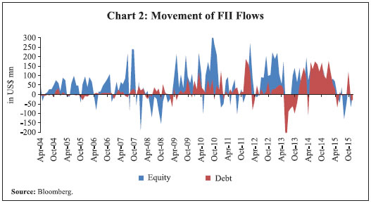 Capital flows to EMEs surged after the global financial crisis, but they remained volatile. EMEs have argued that UMPs of AEs were primarily responsible for the huge inflow of capital to these economies (Ahmed and Zlate, 2013). To analyse whether growth in global liquidity generated by the expansionary monetary policies of AEs has affected financial flows to India, one must look at the definition indicated in BIS (2011), which divide global liquidity into official liquidity and private liquidity. The official liquidity is the summation of global monetary aggregates, while the private liquidity is the summation of global credit aggregates. In the present study, the official liquidity indicator, measured based on the methodology prescribed in Baks and Kramer (1999), is used. First, the monthly money supply growth for the G4 countries (the US, euro area, the UK and Japan) is calculated. The growth rate of money supply for each G4 country (in domestic currency terms) is weighted by the respective country’s GDP share (taken in US dollars) (Kumar and Sharma, 2014). The annual share is applied across all 12 months. In the second step, the weighted GDP growth is obtained for the G4 countries, at a quarterly frequency, where the quarterly growth rate of nominal GDP (in local currency) for each country is weighed by its GDP share in total GDP of the G4 countries (calculated in US dollars). The weighted money supply growth (annualised) in G4 countries gets subtracted by the weighted nominal GDP growth (annualised) in these countries to arrive at the global liquidity growth. The data on narrow money (M2) are used to calculate the money supply growth. The effects of global liquidity are transmitted to EMEs via liquidity, portfolio balance and confidence channels (Lim et al., 2014; Lim and Mohapatra, 2016). First, the liquidity channel operates when the central banks in AEs increase their asset purchases from the market. It operates through both improved availability of liquidity with the banks, as well as lowering of the cost of liquidity in the market. The increased amount of liquidity also reduces the interest rates - many research papers have used the three-month US Treasury Bill yield as an indicator of the liquidity channel. Second, the portfolio balance channel operates through purchase of long duration assets that may alter the demand for financial assets of EMEs, given the possibilities of asset substitution. The difference between interest rate at the long end of the spectrum in a developed country and in India is used as the indicator of this channel. Third, for the confidence channel, sending signals is pertinent. By opting for asset purchases, the central banks try to send signal to the market that the purchase of financial assets can go on till lasting recovery arrives. Hence, the rise in confidence through this process helps in improving the sentiments for investment globally. Here, CBOE VIX is used as the indicator to gauge the market aversion for investment in risky EME assets. In this context, the recent IMF estimates show that normalisation by the US Fed – raising the policy interest rate and shrinking of the balance sheet – is likely to reduce portfolio inflows to emerging markets by about US$70 billion over the next two years as compared with the average annual inflows of US$240 billion since 2010. It estimates that the reduction in the size of the Fed’s balance sheet would cut flows by US$55 billion over the next two years. Flows could fall by an additional US$15 billion if short-term interest rates were to rise in line with the IMF forecasts assuming that the US policy rate would rise to just under 3 per cent by the end of 2019, and that the tightening process would be orderly and would not take a toll on emerging markets growth (IMF, 2017) . Before examining the relationship between global liquidity growth and FII flows to India, it is useful to look at the charts plotting the FII inflow to India along with global liquidity, interest rate differential and global VIX. It is evident from the charts that in the period before 2012, FII inflows to India did not move in tandem with the rise or fall in global liquidity. However, recently there have been occasions showing some correspondence, an indication that global liquidity may lead to FII inflows to India (Chart 3a). The total capital flows to India also show some correspondence with global liquidity growth in the similar manner. The FII inflows rise with the fall in VIX, and vice-versa, though the inverse movement between FII inflows and VIX is less visible in the recent period (Chart 3b). The total capital flows do not show similar association with the VIX. Chart 3c shows that there is no co-movement between FII inflows and interest differentials (id), i.e., difference between the yield on10-year security of the Governmnet of India (GoI) and that of the US.
Section IV
Estimation of the Effects of Global Liquidity on Financial Flows to India Drawing from the literature on the subject (Cerutti et al., 2014; Gordon and Gupta, 2003; Lim et al., 2014; Lim and Mohapatra, 2016), which identified the role of global liquidity, risk aversion/uncertainty, and monetary policy in the AEs in affecting financial flows to EMEs, we estimate the following equation: Net FII flows in the current period is the dependent variable. The independent variables are as follows: (i) FIIt-1 is FII inflow at one period lag, (ii) GLt-1 is the measure of global liquidity at one period lag, (iii) IDt-1 is the interest rate differential at one period lag, (iv) VIXt-1 is the measure of global risk aversion at one period lag. The interest rate differential is calculated by subtracting the average yield on the 10-year government securities of the G4 countries from the GoI 10-year security yield. The regression equation indicates that FII flows to India take place through observable global liquidity (GL), portfolio balance (i.e., ID), and confidence (i.e., VIX) channels. Some more variables are also used in the above equation as additional controls, namely, growth in Index of Industrial Prodouction (IIP) in India, inflation in India, and import-cover of forex reserves to obtain more robust regression results. Furthermore, a dummy has been added for the months when the taper announcement was made by the Federal Reserve (from May to November 2013). Variables are taken in lags to avoid any possibility of endogeneity (Gordon and Gupta, 2003). Data Sources The relevant data for the estimation are sourced from the RBI website (www.rbi.org.in), Securities and Exchange Board of India website (www.sebi.gov.in), Datastream, Bloomberg and Reuters. The money supply (M2) data of the US, the EU, the UK and Japan were obtained from Datastream. The FII flow data are taken from Central Depository Services Ltd. Government security yield and VIX data are taken from Bloomberg. The IIP data for India are taken from the website of the Central Statistics Office (www.mospi.gov.in). GDP data for the US, the EU, the UK and Japan are taken from the OECD Stat database. The net capital/portfolio flows are the dependent variables. At the disaggregated level, flows of FDI, FII, and external commercial borrowings (ECBs) are also separately used. Data periodicity is monthly, from January 2012 to December 2015 (48 data points for the study). The FIIs access to the debt segment was very limited until very recently, though they were allowed as early as in 1998. At the end of 2015, the limits on FPI participation in government securities was US$ 25 billion while in corporate bonds it was US$ 51 billion; the corresponding limits at the end of 2011 were US$ 15 billion and US$ 30 billion, respectively. Empirical Results Sensitivity to Global Liquidity Different types of financial flows exhibit varying sensitivity to different channels of transmission. To study this aspect, capital flows are examined for three major types of financial flows, viz., FDI, FII and ECBs. The ADF test results show that the variables considered are stationary, except the interest rate differential (See Annex II, Table A.1). Hence, the auto regressive distributed lag (ARDL) bounds test is applied to examine the presence of any long-run relationship of different types of capital flows with various channels of global liquidity transmission, and longer period data from January 2001 to December 2015 have been used. The results show that FDI flows and ECBs are not co-integrated with global liquidity (see Annex II, Table A.2). In contrast, and as expected, net FII flow is co-integrated with global liquidity. This result is in line with findings of other studies on portfolio flows to EMEs. The literature indicates that since monetary policy is effective in the short run and portfolio flows are generally short-term in nature, it is likely that these get affected by the monetary policy (Lim et al., 2014; Lim and Mohapatra 2016). FDI is not sensitive to change in global liquidity as it is more dependent on the long-term growth potential of the country. Similarly, ECBs, subject to various regulatory parameters, are not found to be sensitive to global liquidity. Determinants of FII Flows Taking the above approach to a more disaggregated level to empirically examine the determinants of FII flows into India, the same equation is re-estimated while including additional variables – IIP of India (expected sign positive); NEER (expected sign positive); inflation in India (expected sign negative); and, import cover (expected sign positive). Some of the variables are integrated of order one, hence variables in first difference were used to make them stationary. The regressions are estimated by ordinary least square (OLS) with Newey-West heteroskedasticity autocorrelation consistent standard errors and covariance. The regression was estimated using monthly data from January 2012 to December 2015. The lagged dependent variable is always significant. Furthermore, the results show that global liquidity is a significant factor in explaining FII flows to India (see Annex II, Table A.3). It also turns out to be a significant factor in the regression for equity flows, but not for debt flows. However, the p-value of global liquidity is at the margin of 10 per cent in case of debt flows. Overall, the results suggest that the liquidity channel matters for financial flows to India, which in turn indicates that the normalisation of the Fed balance sheet can reduce portfolio flows into India. Other variables like ID and VIX are not statistically significant implying that the portfolio balance channel and the confidence channel do not significantly influence FII flows. Taper dummy is significant in case of total FII flows as well as debt flows Change in import cover is found to be significantly associated with total FII flows and equity flows, but not with debt flows. In contrast with established perception, inflation is found to be positively associated with equity flows into India, which may be incidental. The literature suggests that global liquidity predominantly originates from the US (Cerutti et al., 2014) . It poses questions on the role of other financial centres in the generation of global liquidity. To examine this aspect, the specification used in Annex II, Table A.3 was modified by substituting global liquidity, interest rate differential, and VIX by the liquidity generated in respective countries, interest rate differential of India vis-à-vis the respective country’s 10-year Government security yield (10-year US Government security, 10-year German Government security for Euro, 10-year UK Government security and 10-year Japan Government security) and volatility index in the stock market of the respective countries, viz., US (CBOE VIX), UK (FTSE 100 Volatility), Japan (NIKKEI Volatility) and Euro area (DAX volatility). Other variables in the regression equation as well as the structure of the equation remained the same. As shown in Annex II, Table A.4, the coefficient of liquidity generated in the US was the only statistically significant variable, indicating that liquidity generated in the US is a potent factor in steering FII flows to India while the same does not seem to hold for liquidity originating from the UK, the euro area and Japan. Section V
Conclusion The global crisis of 2008 resulted in a major disruption in the global financial markets. To keep markets alive and running, major central banks adopted UMPs and, as a result, the balance sheets of major central banks expanded exponentially. Between 2007 and 2015, the balance sheets of the European Central Bank and the Bank of Japan doubled, while that of the Federal Reserve of the US and the Bank of England expanded five times. These policies injected a surfeit of liquidity in the markets of the AEs which led to spillovers in the form of capital flows to the EMEs. The reversal happened in a major way in 2013 against the backdrop of the announcement by the Federal Reserve on the reduction of bond purchases or the 'beginning of taper'. The recent announcements on balance sheet normalisation by the Federal Reserve and reduction of monetary stimulus by the European Central Bank have made the global liquidity a more prominent factor to drive capital flows to EMEs. During periods of global market turbulence, financial flows to India have been affected differently. During the period of global financial crisis, an outflow of capital took place, mostly from the equity segment, while during the financial market turbulence generated by the taper talk in 2013, outflows were mostly from the debt segment. Against this backdrop, this paper studied the effects of fluctuations in global liquidity on portfolio flows into India. Empirical findings of this paper point to three broad conclusions: First, global liquidity has differential effects on different types of capital flows. FDI and ECBs are not sensitive to changes in global liquidity conditions while FII flows are sensitive to policies that affect global liquidity. Second, the transmission of global liquidity to India happens through the liquidity channel. This paper does not find any statistically significant role of the other two channels of transmission, i.e., the portfolio balance channel and the confidence channel. Third, the US monetary policy and associated global liquidity conditions exert larger influence on portfolio inflows into India than those of other major central banks.
References Ahmed, S. and A. Zlate (2013), ‘Capital Flows to Emerging Market Economies: A Brave New World?’, International Finance Discussion Papers, No. 1081, June, Board of Governors of the Federal Reserve System. Baks, K. and C. Kramer (1999), ‘Global Liquidity and Asset Prices: Measurement, Implications, and Spillovers’, IMF working paper, No. 168. Basu, K., B. Eichengreen and P. Gupta (2014), ‘From Tapering to Tightening: The Impact of the Fed’s Exit on India’, Policy Research working paper, no. WPS 7071, Washington DC, World Bank Group. Bank for International Settlements (BIS) (2011), ‘Global Liquidity: Concept, Measurement and Policy Implications’, Committee on the Global Financial System (CGFS) Papers, No. 45. Bruno, V. and H. S. Shin (2013), ‘Capital Flows, Cross-border Banking and Global Liquidity’, Griswold Center for Economic Policy Studies, working paper, No. 237a. Cerutti E. M., S. Claessens and L. Ratnovski (2014), ‘Global Liquidity and Drivers of Cross-border Bank Flows,’ IMF working paper, No.14/69. Chandrasekhar, C. P. (2008), ‘Global Liquidity and Financial Flows to Developing Countries: New Trends in Emerging Markets and their Implications’, G24 discussion paper series, No. 52. Chakrabarti, R. (2001), ‘FII Flows to India: Nature and Causes’, Money and Finance, Volume 2, No. 7, October–December. Dua, P. and R. Garg (2013), ‘Foreign Portfolio Flows to India: Determinants and Analysis’, Centre for Development Economics, Delhi School of Economics, working paper, No. 225. Eichengreen, B. and P. Gupta (2015), ‘Tapering Talk: The Impact of Expectations of Reduced Federal Reserve Security Purchases on Emerging Markets’, Emerging Markets Review, Volume 25, Pages 1-15. Forbes, K. J. and F. E. Warnock (2011), ‘Capital Flow Waves: Surges, Stops, Flight and Retrenchment’, NBER working paper, No.17351. Fratzscher, M., M. L. Duca and R. Straub (2013), ‘On the International Spillovers of US Quantitative Easing’, ECB working paper, No. 1557. Gordon, J. P. F. and P. Gupta (2003), ‘Portfolio Flows into India: Do Domestic Fundamentals Matter?’, IMF working paper, No. 3/20. Global liquidity, Credit and Funding Indicators - IMF Policy Paper, 2013 July. Reserve Bank of India (RBI) Handbook of Statistics on Indian Economy, Reserve Bank of India, Mumbai, September 15, 2017. International Monetary Fund (IMF) (2017), Global Financial Stability Report. Kaur, M. and S. S. Dhillon (2010), ‘Determinants of Foreign Institutional Investors’ Investment in India’, Eurasian Journal of Business and Economics, 3(6). Kumar, R. and S. Sharma (2014), ‘Global Liquidity, Financialisation and Commodity Price Inflation’, RBI working paper, No. 1 Lim, J. J., S. Mohapatra and M. Stocker (2014), ‘Tinker, Taper, QE, Bye? The Effect of Quantitative Easing on Financial Flows to Developing Countries’, Policy Research working paper, No. 6820, World Bank. Lim, J. J. and S. Mohapatra (2016), ‘Quantitative Easing and the Post-crisis Surge in Financial Flows to Developing Countries’, Journal of International Money and Finance, Volume 68, 331–357. Mukherjee, P., S. Bose and D. Coondoo (2002), ‘Foreign Institutional Investment in the Indian Equity Market: An Analysis of Daily Flows during January 1999–May 2002’, Money and Finance, Volume 2, No. 9–10. Patra, M. D., J. K. Khundrakpam, S. Gangadaran, R. Kavediya and J. M. Anthony (2014), ‘Responding to QE Taper from the Receiving End’, Journal of Macroeconomics and Finance in Emerging Market Economies, Routledge, Volume 9, No. 2, 167-189. Patra, M. D., S. Pattanaik, J. John and H. Behera (2016), ‘Global Spillovers and Monetary Policy Transmission in India’, RBI working paper, No. 3. Passari, E. and H. Rey (2015), ‘Financial Flows and the International Monetary System’, NBER working Paper, No. 21172. Pesaran, M. H., Y. Shin and R. J. Smith (2001), ‘Bounds Testing Approaches to the Analysis of Level Relationships’, Journal of Applied Econometrics, 16(3), 289–326. Rai, K. and N. R. Bhanumurthy (2004), ‘Determinants of Foreign Institutional Investment in India: The Role of Return, Risk, and Inflation’, The Developing Economies, 42(4), 479-493. Rey, H. (2015), ‘Dilemma not Trilemma: The Global Financial Cycle and Monetary Policy Independence’, NBER working paper, No. 21162. Shankar, A. (2011), ‘QE-II and FII Inflows into India: Is there a Connection?’, RBI working paper, No. 19. Smaghi, L. B. (2009), ‘Conventional and Unconventional Monetary Policy’, Keynote lecture at the International Centre for Monetary and Banking Studies, Geneva, April 28. Verma, R. and A. Prakash (2011), ‘Sensitivity of Capital Flows to Interest Rate Differentials: An Empirical Assessment for India’, RBI working paper, No. 7.
ANNEX I | Some Important Research Papers Published on FII Flows to India | | Authors (Year) | Major Global Variables | Major Domestic Variables | Major Regional Variables | Data Frequency | Indicator for FII Inflow | Methodology Used | | R. Chakrabarti (2001) | S&P 500 Index, MSCI World Index | BSE return (both dollar and Rupee), Volatility of daily US dollar return, Short term interest rate, Credit rating | Nil | Mostly monthly | FII flow as proportion of the preceding month’s market capitalisation | OLS with Newey-West heteroskedasticity autocorrelation consistent standard errors and covariance | | Gordon and Gupta (2003) | IIP in OECD, US stock market return and LIBOR | IIP India, Exchange rate depreciation, Credit rating, Liquidity in BSE, and Seasonal dummies for first four months of the calendar year | MSCI EM Index, IIP in EM | Monthly | FII equity flows in US$ mn, also as a percentage of BSE market capitalisation | OLS corrected through Cochrane-Orcutt two step method | | Mukherjee, Bose and Coondoo (2002) | S&P 500 (return and volatility) MSCI WI(return and volatility) | Market capitalisation in stock market, Sensex (return and volatility), Rupee-dollar exchange rate Call money rate and IIP | – | Daily, return in dollar term in competing markets | FII Purchase to previous day’s market capitalisation (Mcap), FII Sale to previous day’s Mcap, FII Net to previous day’s Mcap | OLS | | Kaur and Dhillon (2010) | S&P 500 return, PPI in USA, US 3 month Tbill rate | Indian stock market return, BSE stock market turnover, Market capitalisation in BSE, WPI, IIP and Exchange rate | – | Monthly | FII net investment | ARDL Model | | Dua and Garg (2013) | IIP growth of OECD countries, 3month Libor | Sensex, NEER, Reserve to Import Ratio, IIP growth in India, interest rate differential (3 month Tbill rate-3 month Libor) and NEER volatility | Morgan Stanley Capital International Emerging Markets Net Index (MSCI-EM) | Monthly | Net FPI,FII, ADR Flows | ARDL Model | | Rai and Bhanumurthy (2004) | S&P 500 Index, PPI USA | BSE Sensex, Monthly standard deviation of sensex and S&P500 and WPI India | – | Monthly | Net FII Flows | TARCH model | | Patra et al (2014) | US IIP, 3 month T-Bill rate in US, Global VIX | India IIP, Rupee-USD rate, trade balance, 10 year yield differential between US and India, 3 month yield differential between US and India, Market capitalisation and WPI inflation | – | Monthly | Gross FII flows | GMM model | Note: S&P 500 : Standard and Poor’s 500
MSCI world Index: Morgan Stanley Capital International World Index
IIP: Index of Industrial production in India
Libor: London Inter-bank Offer rate
PPI : Producer Price Index in USA
NEER: Nominal Effective Exchange rate | ANNEX II | Table A.1: ADF test | | Series | Test statistic | Test Critical value at 5 per cent | Test Critical value at 10 per cent | Result | | Global Liquidity | -11.0 | -2.88 | -2.58 | Unit root rejected | | VIX | -3.93 | -2.88 | -2.58 | Unit root rejected | | ID | -1.10 | -2.88 | -2.58 | Unit root not rejected | | FII flow | -5.90 | -2.88 | -2.58 | Unit root rejected |
Table A.2: Sensitiveness of Types of Capital Flows to Global Liquidity
(ARDL Bounds Test Result for Cointegration) | | Variables | F-statistic | Probability | Result | FII
(FII/ Global Liquidity, Interest Rate Differential, CBOE VIX) | 4.26 | 0.00 | Co-integration | | Critical F value@ | Lower Bound | Upper Bound | | | 95% level | 2.85 | 4.05 | | | 90% level | 2.43 | 3.57 | | FDI
(FDI/ Global Liquidity, Interest Rate Differential, CBOE VIX) | 1.85 | 0.12 | No-cointegration | | Critical F value@ | Lower Bound | Upper Bound | | | 95% level | 2.85 | 4.05 | | | 90% level | 2.43 | 3.57 | | ECB
(ECB/ Global Liquidity, Interest Rate Differential, CBOE VIX) | 2.09 | 0.09 | No-cointegration | | Critical F value@ | Lower Bound | Upper Bound | | | 95% level | 2.85 | 4.05 | | | 90% level | 2.43 | 3.57 | | Note:
@: The critical values are obtained from Pesaran et al., (2001).
#: Lag value of 4 was applied on the basis of AIC criterion, ensuring that there is no serial correlation.
$: In case of FII and FDI, data from January 2001 to December 2015 have been used. Due to the difficulty in data collection, data from April 2004 to December 2015 have been used in case of ECBs. |
| Table A.3: Determinants of Net FII Flows to India during 2012-15 | | Variables | Net FII Flows | Net Debt Flows | Net Equity Flows | | | Coefficient | p-value | Coefficient | p-value | Coefficient | p-value | | Constant | 4.53 | 0.91 | 13.3 | 0.49 | 6.7 | 0.78 | | FII(-1) | 0.50* | 0.01 | 0.42* | 0.02 | 0.41* | 0.08 | | Basic controls | | IIP growth in India(-1) | -5.08 | 0.60 | -0.42 | 0.94 | -4.85 | 0.41 | | Channels of Transmission | | Liquidity channel | | | | | | | | Global liquidity(-1) | 8.5* | 0.00 | 3.14 | 0.10 | 4.9* | 0.00 | | Portfolio Balance channel | | | | | | | | Change in Interest rate Differential (-1) | 79.8 | 0.49 | 47.0 | 0.44 | 24.9 | 0.73 | | Confidence channel | | | | | | | | Change in Global VIX(-1) | 1.77 | 0.88 | 2.21 | 0.67 | -0.69 | 0.91 | | Additional Controls | | Inflation in India(-1) | 40.9 | 0.23 | 1.01 | 0.96 | 38.9* | 0.04 | | Change in NEER(-1) | -10.5 | 0.55 | -8.5 | 0.42 | 3.62 | 0.77 | | Change in Import Cover(-1) | 52.9* | 0.06 | 15.1 | 0.37 | 35.7* | 0.01 | | Taper Dummy | -140* | 0.02 | -105* | 0.00 | -40.8 | 0.20 | | R2 | 0.41 | | 0.45 | | 0.36 | | | Adjusted R2 | 0.27 | | 0.32 | | 0.21 | | | DW statistic | 1.82 | | 1.97 | | 1.63 | | Note: The regressions are estimated by OLS with Newey-West heteroskedasticity autocorrelation consistent standard errors and covariance.
: Variables are statistically significant. |
| Table A.4: Role of Monetory Policy of the US and Other Countries as Drivers of FII flows to India during 2012-2015 | | Variables | US | UK | Euro Area | Japan | | | | | | | | Constant | 40.9 (0.36) | 67.1 (0.08) | 55.9 (0.20) | 63.3 (0.07) | | FII(-1) | 0.47 * (0.03) | 0.42 * (0.03) | 0.40* (0.05) | 0.38* (0.04) | | Basic controls | | IIP growth in India (-1) | -5.77 (0.55) | -9.25 (0.28) | -10.28 (0.18) | -8.24 (0.29) | | Channels of Transmission | | Global Liquidity (-1) | 3.73 * (0.02) | 0.04 (0.98) | 1.72 (0.48) | 1.77 (0.38) | | Change in Interest Rate Differential (-1) | 104.9 (0.39) | 119.7 (0.28) | 65.6 (0.52) | 5.13 (0.52) | | Change in VIX(-1) | 0.34 (0.98) | 0.74 (0.65) | -0.31 (0.87) | 0.10 (0.95) | | Additional Controls | | Inflation in India (-1) | 22.6 (0.50) | 24.1 (0.46) | 23.3 (0.38) | 26.04 (0.47) | | Change in NEER (-1) | -11.8 (0.52) | 2.37 (0.89) | -0.72 (0.97) | 4.51 (0.81) | | Change in Import Cover (-1) | 50.7 * (0.08) | 41.4 (0.14) | 44.8 * (0.08) | 42.7* (0.09) | | Taper Dummy | -140.5* (0.02) | -121.4* (0.06) | -125.5* (0.05) | -121.7* (0.07) | | R2 | 0.39 | 0.35 | 0.34 | 0.24 | | Adjusted R2 | 0.25 | 0.21 | 0.19 | 0.18 | | DW statistic | 1.90 | 1.87 | 1.91 | 1.87 | Note: The regressions are estimated by OLS with Newey-West heteroskedasticity autocorrelation consistent standard errors and covariance. The figures given in the parentheses are the p-values.
: Variables are statistically significant . |
|