Anupam Prakash, Avdhesh Kumar Shukla, Chaitali Bhowmick and
Robert Carl Michael Beyer* In view of the growing popularity of night-time luminosity as a measure of economic activity, this study explores the scope for using such data as a supplement for gross domestic product (GDP) in the Indian context. We found that night-light data exhibit reasonably robust correlataion with GDP and other important macroeconomic indicators like industrial production and credit growth at the national level. Quarter-on-quarter growth of night lights tracks growth of GDP reasonably well. Even after controlling for seasonal factors, the relationship of night lights with value-added in agriculture and private consumption expenditure turns out to be statistically significant. In addition, night lights are strongly correlated with gross state domestic product (GSDP). The elasticity of night lights with respect to GSDP (i.e., the so-called inverse Henderson elasticity) is found to be statistically significant, though relatively smaller in magnitude than similar estimates available at the global level. JEL Classification : E58, O33, O47, R11 Keywords : Night lights, luminosity, satellites, economic growth, Henderson elasticity, GDP Introduction Night-light data, which provide a numerical measure of brightness of the earth during the night, is a direct result of human activities and hold enormous potential in economic analysis (Basihos, 2016; Doll et al., 2006; Donaldson and Storeygard, 2016; Forbes, 2013; Henderson et al., 2012). Night-light data are found to be particularly useful in countries where the quality of official statistics on gross domestic product (GDP) are released with some time-lag, which also get revised several times subsequently. As is the practice in most other countries, initial releases or advance estimates of GDP in India are often revised, and the estimates are improved gradually through successive revisions with the progressive increase in data coverage. The average absolute revisions in India’s GDP growth numbers since the financial year (FY) 2004-05 has been around 0.7 percentage points (Prakash et al., 2018; World Bank, 2017). The state level data on gross state domestic product (GSDP) are often published with a substantial lag. Further, district-level GDP data are not compiled for all the districts, and even if they are compiled, it is not done on a regular basis. This has encouraged analysts and policymakers to supplement the National Accounts Statistics (NAS) with new and innovative data sources including the use of big data to produce better estimates. In recent years, economists are increasingly turning to data from satellite images as a supplementary measure of economic activity that could help assess the state of the economy before revised estimates of GDP become available (Chakravarty and Dehejia, 2017; World Bank, 2017; Henderson et al., 2012). From a policymaking perspective, night-light data can be useful in several ways. First, policies regarding the allocation of resources through various schemes require detailed information at a disaggregated level, which in most cases may not be available in the form of hard data. In India, for example, the Reserve Bank of India (RBI) performs several developmental roles viz., promoting banking habits through financial outreach programmes, encouraging small savings, or making provision of credit facilities to agriculture, industry and other priority sectors, besides its principal function as a central bank (Subbarao, 2013). A proper assessment of the impact of such initiatives is often hindered due to lack of adequate information at disaggregated level. Given the high degree of spatial granularity, night lights could serve as a useful proxy indicator for measuring economic activity across regions in India. Second, with the availability of high frequency night-light data since April 2012, it could be used as an additional lead indicator to improve short-term projections of economic activity. In a large and geographically diverse country like India, a careful exercise is also required to understand the relationship between night lights and other economic variables. This study primarily complements findings of previous studies by Beyer et al. (2018), Bundervoet et al. (2015) and Henderson et al. (2012) in investigating the relationship between night lights and economic activity in the case of India. In addition to an analysis based on annual data, we analyse quarterly night-light data and their relationship with GDP and other crucial macroeconomic variables, such as industrial production and credit growth. Furthermore, we apply, for the first time, the methodology developed by Henderson et al. (2012) at the subnational level in India to study the long-run relationship between night lights and state-level economic activity for the period from 1992 to 2017. The paper is structured as follows. Section II presents a brief review of the relevant literature. Section III provides a description of the night-light data. Section IV examines the salient features of the night-light data in the Indian context and its behaviour vis-à-vis GDP and other macro-economic variables. Econometric analysis using state-level data is presented in section V. Section VI concludes the paper. Section II A Brief Survey of Related Literature The application of satellite data in understanding issues of social sciences traces back at least to the early 2000s, and therefore is not of a recent origin. One can document numerous studies using such data on topics as diverse as population dynamics, urbanisation, use of natural resources, regional disparities, poverty, inequality, distribution of wealth, relationship between wealth and health indicators, pollution research, and so on (Asher et al., 2017; Economic Survey, Government of India, 2016-17; Donaldson and Storeygard, 2016; Hodler et al., 2014). Night-light data have also been used to examine the impact of various events, for example, major natural catastrophes, policy actions or outbursts of conflict (Beyer et al., 2018; Chodorow-Reich et al., 2018; Bundervoet et al., 2015). In this section, we present a brief survey of the literature which links luminosity with economic output and growth, particularly in the Indian case. Night lights and Economic Growth In a seminal paper, Henderson et al. (2012) use night lights as a tool to augment the GDP series of 188 countries, and motivate research employing night-light data in the field of economics. The elasticity of night lights with respect to GDP, popularly known as the Henderson elasticity, is estimated empirically in a panel regression framework with GDP as a dependent variable and night lights as an explanatory variable along with other relevant variables. The coefficient of night lights is the inverse of Henderson elasticity and it is statistically significant. Henderson et al., (2012) also show how the spatial granularity of the night-light data can provide new insights. For example they find that growth in coastal areas of sub-Saharan Africa was against expectation and lower than growth in hinterland. Luminosity as a proxy of output has also been used to compare the quality of statistical data across countries, both at the country level and at the ‘1° latitude × 1° longitude grid-cell level’ for the period from 1992 to 2008 (Chen and Nordhaus, 2011). Luminosity adds little value for countries with high-quality statistical systems, but is useful in countries with low statistical capacity. Another study comes to a similar conclusion and argues that the measurement of GDP per capita in middle- and low-income countries is less precise and, therefore, night lights can play an important role in improving GDP aggregates of these economies (Hu and Yao, 2018). Interestingly, in the case of China, night lights adjusted GDP growth was found to be lower than the official estimates (Zhou and Zeng, 2018). Similarly, night-light data have been used to compare the accuracy of GDP per capita reported in national accounts vis-à-vis income measures based on surveys in India and Angola, where national accounts data were found to be superior compared with income estimates derived from household surveys (Pinkovskiy and Sala-i-Martin, 2015). The spatial granularity of night-light data is found to be very useful for regional studies. For example, night lights have been used to map regional economic activity in 11 European Union (EU) countries and the United States (US), for which a strong positive relationship has been found between night lights and GDP across a range of spatial scales (Doll et al., 2006). For Turkey, night lights were used to estimate the gross provincial product (GPP) from 2001 onwards, a period for which no official estimates are available (Basihos, 2016). Similarly, the subnational GDP of Kenya and Rwanda were estimated using night-light data (Bundervoet et al., 2015). The correlation between GDP and night lights has also been examined for the Metropolitan Statistical Areas (MSA) of Florida (Forbes, 2013). For these areas, strong correlations with different measures of economic activity within each MSA allow to detect even specific industries contributing most to the variance of night lights. However, a few studies indicate that night lights may not be a good proxy for sub-regional GDP. Bickenbach et al. (2016), for example, tested a hypothesis like the one in Henderson et al. (2012) for long-term growth rates of GDP at the subnational level for Brazil, India, Europe and the US. They conclude that growth elasticities are not stable across the geographies of each country or region. Addison and Stewart (2015) also argue that growth elasticities of night lights with respect to economic activity are too small and unstable over time limiting their utility for any practical use. With the night-light data becoming available at a monthly frequency, some new applications focusing on short-term growth became possible. Bhadury et al. (2018) use night-light data and other high frequency information in a nowcasting model and illustrate that the inclusion of night lights reduces the early nowcast errors in the ‘trade, hotels, transport, communication and services related to broadcasting’ sub-sector of India's gross value added (GVA) estimates. Literature Related to India In India, the relationship between night lights and GDP has been explored at the district level, for which reliable estimates of economic activity are not available. Bhandari and Roychowdhury (2011) use a multinomial regression technique to establish that differences in GDP at the district level are largely captured by night lights. In their case, non-linear models provide better results than linear models, which tend to underestimate GDP in the urban areas and overestimate GDP in areas dominated by agriculture and forestry activities. Another interesting application of night-light data in India is to test for inter and intra-regional convergence/divergence. Chakravarty and Dehejia (2017) show that intra-state divergence across districts is as significant as inter-state divergence. Their analysis reveals that ten out of the twelve largest states exhibit divergence at district-level within the states. Chanda and Kabiraj (2018) employ night-light data to study the divergence of Indian districts both at the aggregate district level as well as along the rural and urban dimension for the period from 2000 to 2010. Contrary to the results reported by other studies such as Chakravarty and Dehejia (2017), Kalra and Sodsriwiboon (2010) and Bandyopadhyay (2012), Chanda and Kabiraj (2016) find evidence of both absolute and conditional convergence in rural areas, but not in the urban areas. In most of the studies related to India, night lights have been used as a proxy for economic activity at the state level or district level. However, to the best of our knowledge, there are hardly any studies which examine the relationship for a longer time horizon after controlling for various state-specific and time-varying effects. Secondly, given the range of economic, social and cultural diversity among Indian states, this study is also a first attempt to understand whether state-specific factors such as sectoral composition, population and income levels have any significant impact on the relationship between night lights and GDP. The objective is to develop a coherent understanding of the nature of the relationship between night lights and GSDP in the Indian context which might provide further direction for future studies in this area in terms of choice of variables and model specification. Section III A Brief Description of the Data Night-light Data Night-light data are basically the visible lights emanating from the earth captured by satellites from outer space. For the period 1992 to 2013, night-light data are publicly available on an annual basis as a by-product of the Defence Meteorological Satellite Program (DMSP) of the United States Department of Defense, which includes a main weather sensor Operational Line Scan System (OLS). It captures night lights daily between 8.30 p.m. to 9.30 p.m. In addition to lights emanating from economic activity, it may also detect lights originating from gas flaring, shipping fleets, auroral activity, forest fires, etc. Therefore, the National Oceanic and Atmospheric Administration (NOAA) has developed an algorithm which allows it to identify stable lights by removing sunlit, glare, and moonlit (Addison and Stewart, 2015). Luminosity is measured by a digital number on a linear scale between 0 and 63. The numbers are then aggregated to arrive at the sum of lights for a geographical location. Night-light intensity for an area is then obtained by dividing the sum of light by total size of the area. One limitation of this data is that there is an upper limit of 63, which implies that in case a number 63 gets assigned, any further growth in the light would not be captured. For South Asia, however, this is not a problem as only very few metropolitan areas are that bright. From April 2012 onwards, a new data product became available at monthly frequency from a different satellite programme called the Suomi National Polar Partnership Satellite with a Visible Infrared Imaging Radiometer Suit (SNPP-VIIRS). Apart from being available at a higher frequency, this data-set has some improved features compared to the DMSP-OLS data. For example, as the unit of measurement is nanowatt, there is no upper limit in the case of DMSP-OLS data. The data available in the public domain still include some temporary lights and background noise. Hence, we use cleaned VIIRS night-light data based on Beyer et al. (2018) in this study. Advantages and Limitations of the Night-light Data There are some major advantages of night-light data as a measure of economic activity. First, as the data are available at monthly frequency, it provides a useful alternative for data that come with a lag. Second, it gives more freedom to researchers due to their availability beyond state borders. Third, it is available at a more granular level. Besides, one major advantage of night-light data is that one can altogether escape the difficulty of measuring informal activities as it captures economic activities regardless of whether it is formal or informal. Moreover, there is no scope for subjective interference and the cost of acquisition is also less. Finally, measurement errors of official GDP estimates are uncorrelated with the errors resulting from physical conditions affecting luminosity record quality. Despite several advantages, night-light data are, however, no silver bullet for solving all issues related to the measurement of economic activity. The data are noisy and the relationship between night lights and economic activity is also not homogenous. Night-light intensity depends on various exogenous and endogenous factors such as the level of electricity generation, the sectoral composition of output, and the existing level of development. All these factors tend to vary across time and space. For example, at the global level, the responsiveness of night lights intensity to changes in the manufacturing sector are found to be larger than that of changes in the services sector. For South Asian countries, however, the opposite result is observed (World Bank, 2017). In addition, for South Asian countries, night lights seem to be a poor indicator of activity of the agricultural sector, as agricultural activities mostly take place during the day and hence may emit less light. Therefore, one may expect that night lights may not be a good indicator of economic activity in rural areas with higher share of agricultural output. Moreover, electricity generation capacity emerges as a major determinant of night-light intensity of any region. At early stages of development, when power sector infrastructure develops at a fast pace, night lights growth tend to be high. In more developed regions, where power infrastructure is already in place, the rate of growth of night lights may be lower. In view of the above considerations, one needs to carefully assess various other time-specific and region-specific factors. Other Data used in the Study Along with night-light data, official statistics such as real GDP, real GSDP, sectoral GVA, and the Index of Industrial Production (IIP) published by the National Statistical Office (NSO), as well as real money and credit data published by the RBI are used in our study. For the panel regression analysis, we use real net state domestic product (NSDP) at factor cost up to 2010-11 and real net state value added (NSVA) at basic prices from 2011-12 onwards, as historical time series data on GSDP are not available. One caveat is that while GDP and GSDP data are available on a financial year basis (April to March), the annual night-light data prior to 2013 are available on a calendar year basis (January to December)1. This problem is overcome for the later years (i.e., 2013 onwards), for which monthly night-light data are available. Section IV Night lights and GDP: An Assessment at the National Level This study examines some basic features of night-light data and its relationship with GDP and other macroeconomic variables. We first examine a few standard time series properties of the annual night-light data for India from 1992 to 2017, followed by an examination of the quarterly data from 2012 onwards. Both the natural logarithm of GDP2 and the sum of night lights portray a linear upward trend (Chart 1). A closer look at the growth trajectory separately for each decade of the period covered in this study suggests that the long-run average growth in real GDP and night lights moved in close proximity to each other (Table 1). For the overall period (1992 to 2017), average annual growth in GDP and night lights were 6.5 per cent and 7.1 per cent, respectively. Quarterly figures of night lights from the first quarter of 2012 to the second quarter of 2017 have been generated from the monthly VIIRS night-light data. The quarter-on-quarter (q-o-q) movement in GDP clearly depicts a seasonal pattern with a peak in October to December quarter and a trough in April to June (Chart 2). The seasonal movement in night lights captures the seasonal variations in GDP quite closely. Prima facie, it turns out that night lights track both trend and seasonal variations in GDP.
| Table 1: Average Annual Growth Rates in GDP and Night Lights | | (in per cent) | | Variable | 1993–2002 | 2003–2012 | 2013–17 | 1992–2017 | | GDP | 5.8 | 7.0 | 7.1 | 6.5 | | Night lights | 6.1 | 8.5 | 6.6 | 7.1 | | Source: NSO, DMSP-OLS and VIIRS. | Next, we examine how night lights relate to other macroeconomic variables in India. Night lights exhibit strong correlation with some other major macroeconomic variables as well. Table 2 presents the correlation coefficient matrix of night lights, GDP, non-agricultural GDP, industrial production (general, electricity, and manufacturing), money and credit growth. The correlation coefficient between night lights and overall GDP is 0.75 and with non-agricultural GDP it is 0.55, both the coefficients being statistically significant at the 5 per cent level. Night lights also relate reasonably well to industrial production. The correlation of night lights with money supply and credit flows is also strong and statistically significant. Strong and statistically significant correlation coefficient of night lights with some important macroeconomic indicators further strengthens the case for night lights to qualify as an indicator of economic activity. Though correlation between night lights and other macroeconomic variables is strong in levels, it is significantly weaker with regards to growth rates. 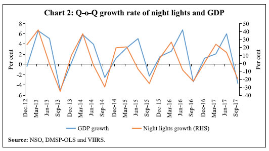
| Table 2: Correlation Matrix (June 2012 – December 2017) | | Variables | Night lights | GDP | Non-agri GDP | IIP-Gen | IIP-E | IIP-M | Real M4 | Real credit | | Night lights | 1 | | | | | | | | | GDP | 0.75* | 1 | | | | | | | | Non-agri GDP | 0.55* | 0.94* | 1 | | | | | | | IIP-Gen | 0.75* | 0.99* | 0.91* | 1 | | | | | | IIP-E | 0.56* | 0.89* | 0.96* | 0.84* | 1 | | | | | IIP-M | 0.72* | 0.98* | 0.91* | 0.99* | 0.84* | 1 | | | | Real M4 | 0.66* | 0.98* | 0.96* | 0.95* | 0.94* | 0.94* | 1 | | | Real credit | 0.68* | 0.98* | 0.95* | 0.96* | 0.93* | 0.95* | 0.99* | 1 | *: Indicates statistically significant at 5 per cent level.
Note: Correlation coefficients between the variables are calculated at levels.
Source: NSO, the RBI and VIIRS. | As established above, q-o-q growth of night lights track q-o-q growth of GDP reasonably well. However, one may suspect that night lights and GDP may both be driven by seasonality and time-trend factors. To control for seasonality, following Wooldridge (2012), we regress q-o-q GDP growth and q-o-q night-light growth on quarterly dummies, and then regress the residuals of the GDP growth regression equation on the residuals of the night-light regression equation. The coefficient of this regression equation reveals the impact of night lights on q-o-q GDP growth rate. Next, we include a time trend in the regression. We regress quarterly GDP, GVA and GVA of agriculture and allied activities, as well as private final consumption expenditure on q-o-q growth rate of night lights (Tables 3a and 3b). | Table 3a: Regression Results of Residuals of Q-o-Q GDP Growth and its Components on Residuals of Night lights after Controlling Seasonality | | Variables | GDP | GVA | Agriculture and Allied Activities | PFCE | | Residuals of night lights | 0.088*** | 0.074*** | 0.196*** | 0.067* | | | (0.016) | (0.014) | (0.038) | (0.035) | | Constant | 0.000 | 0.000 | -0.000 | 0.000 | | | (0.206) | (0.217) | (0.458) | (0.428) | | Observations | 22 | 22 | 22 | 22 | | R-squared | 0.463 | 0.358 | 0.464 | 0.103 | ***: p<0.01; **: p<0.05; *: p<0.1.
Note: The figures in parentheses are robust standard errors. | In all the cases, the coefficient of night lights is statistically significant with a positive sign. The results for GVA as well as agriculture and allied activities are particularly interesting as they suggest a stronger relationship with night lights. The coefficient of night lights for agriculture is positive and higher in magnitude than that of GDP. This finding is against the hypothesis that night lights may not adequately capture the changes in agricultural growth. | Table 3b: Regressions Results of Residuals of Log of GDP and its Components over Residuals of Log of Night lights after Controlling Seasonality and Time-trend | | Variables | GDP | GVA | Agriculture and Allied Activities | PFCE | | Residuals of night lights | 0.039** | 0.043** | 0.152*** | 0.004 | | | (0.018) | (0.020) | (0.047) | (0.023) | | Constant | 0.000 | -0.000 | 0.000 | 0.000 | | | (0.002) | (0.002) | (0.004) | (0.003) | | Observations | 23 | 23 | 23 | 23 | | R-squared | 0.101 | 0.132 | 0.254 | 0.001 | ***: p<0.01; **: p<0.05; *: p<0.1.
Note: The figures in parentheses are robust standard errors. | In the case of private final consumption expenditure (PFCE), we also observe a positive and statistically significant coefficient. A possible explanation of these results is that agricultural production is the major determinant of India’s consumption demand. Additionally, harvesting seasons also coincide with major Indian festivals when use of night lights increases. Overall, the results show that night lights do have statistically significant predictive power for economic activity in India even after controlling for seasonal factors. Section V Econometric Analysis at the Level of States In this section, we examine whether night lights provide any insights on the behavior of macroeconomic variables at the sub-national level. A scatter plot of the logarithm of gross state value added (GSVA) and the logarithm of night lights for 32 states and union territories for the financial year 2015-16 indicates a strong positive relationship between the two variables (Chart 3). These observations yield a high correlation coefficient of above 0.7 between GSVA and night lights. For other years too, we find very similar results. The above discussions suggest that based on night-light data for a given state, one can predict GSVA for that state. The efficiency of the prediction may, however, depend on state-specific characteristics. We, therefore, examine if there exists a relationship between the prediction errors, defined as the national account estimate minus the prediction based on night lights, and state-specific characteristics, viz., the population density, the income level, and the share of agriculture in GSVA. Scatter plot of errors from the predicted GSVA and state characteristics are given in Chart 4. Interestingly, the prediction error rises with population density which means that in more densely populated states, predictions based on night lights alone will result in an under-estimation of GSVA. With increase in population density, the amount of GSVA per unit of light increases. In other words, in more densely populated states, each unit of GSVA is associated with lesser night lights compared to sparsely populated states. The relationship between the prediction error and the population density is found to be significant at 1 per cent level. Regarding the per capita income levels and shares of agriculture in GSVA, none of them systematically affects the prediction errors. The scatter plots indicate that the amount of GSVA per unit of light does not increase with income per capita and hence gives some confidence that night lights can approximate GSVA across all states in India, independent of the income level. For the share of agriculture in GVA, there is a weak relationship wherein with a higher share of agriculture, the prediction based on night lights tends to over-predict GSVA. However, this relationship is not statistically significant, which indicates that night lights are able to predict economic activity independent of the sector generating the value added. This is in line with the regression results presented in Table 3. It reassures that the amount of night lights and economic activity at the state level are strongly correlated. However, to use night lights as a credible measure of economic activity, one needs to establish that the changes in economic activity translate into changes in night lights. The question, therefore, is whether more economic activity in a state is associated with more night lights and, if so, then how strong this relationship is. In other words, we are interested in the elasticity of night lights with respect to changes in state economic activity. Following the methodology developed by Henderson et al. (2012), we estimate a panel regression for Indian states which will provide the elasticity of night lights with respect to state level economic activity. We estimate different variants of the following baseline model: where ln(Yc,t) is the natural logarithm of economic activity of state c in year t, measured at constant prices, ln(lintensityc,t) is the natural logarithm of light brightness per km2, bc represents state fixed effect, ct represents a year fixed effect, and εc,t is the random error component. The state fixed effect controls for differences among states in terms of cultural specificities,sectoral composition, etc. The time trend captures sensor ageing and changingtechnologies.3 We estimate the above model, first for the sub-period from 1992 to 2013using only the clean annual data from the DMSP-OLS series. Next, we use aspliced series of night lights that extend the DMSP-OLS series with VIIRSdata following Beyer et al. (2018). This allows us to estimate the model forthe full sample period from 1992 to 2017. The results are presented in Table 4. The first variant of the model, given in Column 1, does not include a time trend. Since both series have increasing trends (as described above), the coefficient is very high. In the second variant of the model given in Column 2, we include a time trend, which makes this regression identical to the one specified above and the one estimated for the world by Henderson et al. (2012). The coefficient of night lights is 0.15 and it is statistically significant at the 10 per cent level. The magnitude of the coefficient is only half of what Henderson et al. (2012) find for the world and the one that Beyer et al. (2018) find for South Asia. Next, we include the squared night lights as a variable to account for the possibility of a non-linear relationship. While the squared term itself is not statistically significant, it strengthens the significance of the linear coefficient of night lights to the 5 per cent level. Even though we do not find a significant relationship between the income level and the errors from predicting NSDP based on night lights, the elasticity may still depend on the income level. Indeed, it has been argued that the elasticity increases with higher income levels, at least for low and medium income regions (World Bank, 2017). To account for this possibility, we next include an interaction term of night lights and per capita NSDP. Results, reported in Column 4, are found to be in line with the hypothesis that the relationship strengthens with higher income per capita. The model is estimated for the full sample period (1992-2017) and the results are reported in Columns 5 to 8 in Table 4. They suggest that the relationship between economic activity and night lights measured by DMSP-OLS and night lights measured by VIIRS may be different. The coefficient for night lights in Columns (6) and (7) are not statistically significant even at the 10 per cent level. This may very well be due to a change in the relationship caused by the switch from DMSP-OLS to VIIRS. However, when the interaction term between lights and income per capita is included in the model, the coefficient turns out to be statistically significant again. So far, VIIRS data exists only for five years and hence no separate relationship can be estimated using just VIIRS data. In the future, as more data from VIIRS become available, it will be interesting to test for a structural break in this relationship. | Table 4. Henderson Elasticity for Indian States | | Item | 1992–2013
DMSP-OLS | 1992–2017
DMSP-OLS & VIIRS | | (1) | (2) | (3) | (4) | (5) | (6) | (7) | (8) | | Night lights | 0.835*** | 0.149* | 0.180** | 0.175** | 0.874*** | 0.108 | 0.120 | 0.154* | | | (0.0369) | (0.0831) | (0.0826) | (0.0724) | (0.0421) | (0.0900) | (0.0825) | (0.0788) | | Night lights squared | | | 0.0131 | | | | 0.00598 | | | | | | (0.0117) | | | | (0.0133) | | | Night lights # NSDP per capita | | | | 0.870*** | | | | 0.656*** | | | | | | (0.220) | | | | (0.192) | | Constant | 5.971*** | 5.583*** | 5.552*** | 5.587*** | 5.999*** | 5.582*** | 5.567*** | 5.602*** | | | (0.00772) | (0.0418) | (0.0558) | (0.0404) | (0.0136) | (0.0432) | (0.0623) | (0.0431) | | Time trend | NO | YES | YES | YES | NO | YES | YES | YES | | State fixed effects | YES | YES | YES | YES | YES | YES | YES | YES | | Observations | 673 | 673 | 673 | 670 | 785 | 785 | 785 | 782 | | R-squared | 0.649 | 0.945 | 0.946 | 0.954 | 0.713 | 0.950 | 0.951 | 0.957 | | Number of states | 32 | 32 | 32 | 32 | 32 | 32 | 32 | 32 | ***: p<0.01; **: p<0.05; *: p<0.1.
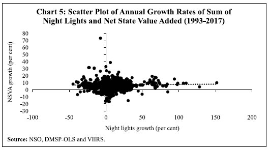
Note: The figures in parentheses are robust standard errors. | Furthermore, the long-run relationship between NSDP and night lights are analysed using panel cointegration tests to check robustness of earlier results. The Im-Pesaran-Shin unit root test for both NSVA and night lights confirms the presence of unit roots and thereby non-stationarity in both the series (Table 5). We, therefore, perform panel cointegration test covering data for 28 states4 and union territories for the period 1992-93 to 2016-17 in order to examine whether the covariance between NSVA and night lights remained constant over time. Both the Kao test and the Pedroni test (which are based on the Engle-Granger two-step cointegration test) for cointegration reject the null hypothesis of no cointegration and therefore confirm existence of a long-run relationship between NSVA and night lights (Table 6). After finding a long-run relationship (at levels) between state economic activity and the sum of night lights, we briefly analyse the relationship between annual GSDP growth and night-light growth. Scatter plot of annual growth rates of the sum of night lights and of state GDP depicts that correlation is close to zero and statistically not significant (Chart 5). | Table 5: Panel Unit Root Test Results | | Method: Im-Pesaran-Shin unit-root test - Number of periods: 25 | H0: All panels contain unit root
Ha: Some panels are stationary | | Variable | t-statistic* | p-value | | Night lights | -0.7482 | 1.0000 | | NSVA | 3.8574 | 1.0000 | | *Critical values at 1 per cent, 5 per cent and 10 per cent are -1.820, -1.73 and -1.690, respectively. |
| Table 6: Panel Cointegration Test Results | | Kao’s Residual Cointegration Test results | | Statistic | Value | p-value | | Modified Dickey–Fuller t | -1.3592 | 0.0870 | | Dickey–Fuller t | 0.0683 | 0.4728 | | Augmented Dickey–Fuller t | 3.6279*** | 0.0001 | | Unadjusted modified Dickey–Fuller t | -1.5553* | 0.0599 | | Unadjusted Dickey–Fuller t | -0.0507 | 0.4798 | | Pedroni’s Residual Cointegration Test results | | Modified Phillips–Perron t | -3.2064*** | 0.0007 | | Phillips–Perron t | -3.9759*** | 0.0000 | | Augmented Dickey–Fuller t | -4.4904*** | 0.0000 | | Westerlund Cointegration Test Results | | Variance ratio | -0.7924 | 0.2141 | | ***: p<0.01; **: p<0.05; *: p<0.1. |
 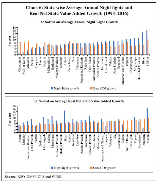 We further plot the average annual growth rates of the sum of night lights and NSVA (Chart 6). Among major states, night lights grew the most during this period in Bihar, Chhattisgarh, Uttar Pradesh and Odisha. However, economic activity in these states grew at a much slower pace. The national capital region Delhi, Gujarat and Haryana recorded the fastest GDP growth during this period, but the night lights growth in these states was found to be relatively low. The high growth in night lights observed in relatively poorer states perhaps reflects the catching up process i.e., the progress being made in terms of electrification of unelectrified households. Section VI Conclusion The analyses presented in this study confirm that night lights are a reasonably robust indicator of economic activity in India as it tracks both trend growth and seasonal variations in GDP reasonably well. In addition, the relationship of night lights with quarterly GDP and its components (viz., GVA-agriculture and allied activities and PFCE) is found to be statistically significant even after controlling for seasonality and time trend. The state-level analysis showed the presence of a long-run cointegrating relationship between night lights and GDP. The prediction precision of state income using night lights may, however, depend on state specific characteristics. For densely populated states, the prediction of economic activity based on night lights alone tends to underpredict the level of activity. For India, we find a statistically significant inverse Henderson elasticity, the magnitude of which is about half of what Henderson estimated at the global level. However, annual growth rates of income of the states and night lights, are found to be uncorrelated. Notwithstanding the presence of a statistically significant relationship between night lights and GDP, there are certain limitations of using night-light data for economic measurement. First, given that it is just a rough approximation of economic activity, it should be considered at best as an additional indicator and not a substitute. Second, although night lights correlate strongly with GDP, the correlation weakens substantially when growth rates are considered, which suggests that one needs to be careful while using night-light data for analysing short-term events. The existing literature finds similar result for other countries as well (World Bank, 2017). Third, night lights as a proxy for economic activity do not distinguish between value added in different sectors. Despite its limitations, the findings of this study suggest that night-light data can be a useful source of information for valuable macroeconomic analysis and research in India, as it is in other countries.
References Addison, D., & Stewart, B. (2015). Nighttime lights revisited: the use of nighttime lights data as a proxy for economic variables. The World Bank. Asher, S., & Novosad, P. (2017). Politics and local economic growth: Evidence from India. American Economic Journal: Applied Economics, 9(1), 229-73. Bandyopadhyay, S. (2012). Convergence clubs in incomes across Indian states: Is there evidence of a neighbours’ effect?. Economics Letters, 116(3), 565-570. Basihos, S. (2016). Nightlights as a Development Indicator: The Estimation of Gross Provincial Product (GPP) in Turkey. Available at SSRN 2885518. Beyer, R. C., Chhabra, E., Galdo, V., & Rama, M. (2018). Measuring districts’ monthly economic activity from outer space. The World Bank. Bhadury, S., Pohit, S., & Beyer, R. C. (2018). A New Approach to Nowcasting Indian Gross Value Added (No. 115). Bhandari, L., & Roychowdhury, K. (2011). Night lights and economic activity in India: A study using DMSP-OLS night time images. Proceedings of the Asia-Pacific advanced network, 32, 218-236. Bickenbach, F., Bode, E., Nunnenkamp, P., & Söder, M. (2016). Night lights and regional GDP. Review of World Economics, 152(2), 425-447. Bundervoet, T., Maiyo, L., & Sanghi, A. (2015). Bright lights, big cities: measuring national and subnational economic growth in Africa from outer space, with an application to Kenya and Rwanda. The World Bank. Chakravarty, P., & Dehejia, V. (2017). Will GST exacerbate regional divergence?. Economic & Political Weekly, 52(25-26), 97-102. Chanda, A., & Kabiraj, S. (2018). Shedding Light on Regional Growth and Convergence in India. Available at SSRN 3308685. Chen, X., & Nordhaus, W. D. (2011). Using luminosity data as a proxy for economic statistics. Proceedings of the National Academy of Sciences, 108(21), 8589-8594. Chodorow-Reich, G., Gopinath, G., Mishra, P., & Narayanan, A. (2018). Cash and the Economy: Evidence from India’s Demonetization (No. w25370). National Bureau of Economic Research. Doll, C. N., Muller, J. P., & Morley, J. G. (2006). Mapping regional economic activity from night-time light satellite imagery. Ecological Economics, 57(1), 75-92. Donaldson, D., & Storeygard, A. (2016). The view from above: Applications of satellite data in economics. Journal of Economic Perspectives, 30(4), 171-98. Forbes, D. J. (2013). Multi-scale analysis of the relationship between economic statistics and DMSP-OLS night light images. GIScience & remote sensing, 50(5), 483-499. Government of India (GoI) (2017). Economic Survey 2016–17, Volume I, February, Department of Economic Affairs, Ministry of Finance Affairs, Government of India. Henderson, J. V., Storeygard, A., & Weil, D. N. (2012). Measuring economic growth from outer space. American economic review, 102(2), 994-1028. Hodler, R., & Raschky, P. A. (2014). Regional favoritism. The Quarterly Journal of Economics, 129(2), 995-1033. Hu, Y., and Yao, J. (2018). “Illuminating Economic Growth”, Working Paper No. 19/77, IMF Working Papers. Pinkovskiy, M., & Sala-i-Martin, X. (2014). Lights, Camera,... Income!: Estimating Poverty Using National Accounts, Survey Means, and Lights (No. w19831). National Bureau of Economic Research. Prakash, A., Shukla, A. K., Ekka, A. P., and Priyadarshi, K. (2018) “Examining gross domestic product data revisions in India”, Mint Street Memo No. 12, Reserve Bank of India. Kalra, S., & Sodsriwiboon, P. (2010). Growth convergence and spillovers among Indian states: what matters? What does not?. IMF Working Papers, 1-34. Subbarao, D. (2013). Five Years of Leading the Reserve Bank Looking Ahead by Looking Back. Tenth Nani A. Palkhivala Memorial Lecture, Mumbai, 29. Wooldridge, Jeffrey M. Introductory Econometrics: A Modern Approach. Mason, Ohio: South-Western Cengage Learning, 2012. World Bank. 2017. South Asia Economic Focus, Fall 2017 : Growth Out of the Blue. Washington, DC: World Bank. © World Bank. https://openknowledge.worldbank.org/handle/10986/28397 License: CC BY 3.0 IGO. Zhou, Qiyao and Zeng, Jiangnan, Promotion Incentives, GDP Manipulation and Economic Growth in China: How Does Sub-National Officials Behave When They Have Performance Pressure? (October 19, 2018). Available at SSRN: https://ssrn.com/abstract=3269645 or http://dx.doi.org/10.2139/ssrn.3269645
|