Sujata Kundu* This paper analyses the trends in rural wages in India during January 2001 to February 2019, with a view to identifying the key factors that could explain the recent slowdown in agricultural wage growth. The paper examines the role of rural prices in explaining wage movements in India and assesses the risk of a wage-price spiral to the inflation trajectory. The results show that agricultural and non-agricultural wages both share a long run positive relationship with rural prices. For the period from November 2013 to February 2019, the paper finds that the changes in rural prices had a positive and significant impact on changes in nominal agricultural wages, even after controlling for other determinants such as non-agricultural wages, Mahatma Gandhi National Rural Employment Guarantee Scheme (MGNREGS) wages, and rainfall departure from normal. The nominal agricultural wages showed stickiness and a significant positive influence of non-farm wages. This paper does not find any robust empirical evidence of a wage-price spiral in India during the period under the study. JEL Classification : J21, J31, E24, E31, E52 Keywords : Rural wage, inflation, MGNREGS, construction wage Introduction Rural wages in India have witnessed sharp movements in the past few years. During the last 10-year period, a high growth phase in rural wages from 2007-08 to 2012-13 was followed by a phase of significant deceleration. Because of a spell of high inflation during October 2015 to September 2016, growth in real agricultural wages slipped into the negative territory and subsequently turned positive but remained low.1 Since rural wages play a major role in determining the living standard of a large section of population in the country, it is worthwhile to examine the factors behind the changing rural wage dynamics and the subdued growth in wages in the recent years. It is crucial to note that two major factors, viz., the implementation of the Mahatma Gandhi National Rural Employment Guarantee Scheme (MGNREGS) and a healthy growth of the construction sector (as measured by the sector’s gross domestic product), that contributed to the high growth phase in rural wages up to 2012-13, have weakened in terms of their significance in the recent period. The high wage growth period also coincided with elevated inflation in the economy. In the post 2012-13 period, inflation has eased significantly, which was also accompanied by a sharp fall in nominal wage growth. For agricultural wages, it has been observed that growth in the agricultural sector influences wages positively (Bhalla, 1979; Himanshu, 2006; Jose, 1974; Lal, 1976; Venkatesh, 2013). The agricultural output growth was subdued during 2014-16 due to sub-normal monsoon. The growth improved during 2016-18 with the normal monsoon. The rural wage growth during these years, however, remained low indicating that the role of agricultural output in influencing rural wages has become limited. While an appropriate understanding of the factors responsible for movements in rural wages is important from the perspective of welfare consequences for the rural economy, it is also crucial to recognise the fact that rural wage dynamics have implications for inflation and overall economic growth in an emerging market economy like India. Most of the early empirical literature on rural labour market in India has looked into various factors determining movements in rural wages at different periods in time. Some of the recent studies have specifically focussed on the upsurge in rural wages between 2007-08 and 2012-13. Some of them have reported the implementation of MGNREGS as an important factor behind the surge in rural wage growth (Chand et al., 2009; Pandey, 2012), while another study found that besides MGNREGS, a healthy performance of the construction sector and general urbanisation trend also led to the upswing (Himanshu and Kundu, 2016). This period was characterised by wages growing at a considerably higher rate than the overall inflation in the economy and many researchers went on to argue that such rise in wages, if unaccompanied by increase in productivity, could induce a wage-price spiral by raising aggregate demand on the one hand and pushing up cost of production on the other (Guha and Tripathi, 2014; Nadhanael, 2012). Rural wage growth moderated noticeably after 2012-13. Although a lot of mainstream media reports have highlighted this fact, a careful and broader analysis of the long-term trends in rural wages is needed. In this backdrop, this paper analyses the trends in rural wages – both farm (agricultural) and non-farm (non-agricultural) wages – in India over the past decade, while trying to identify the possible major factors that could explain the recent slowdown in agricultural wage growth. In particular, the paper tries to examine the role of rural prices in explaining wage movements in India. In comparison to the earlier studies in this area (Goyal and Baikar, 2014; Guha and Tripathi, 2014; Nadhanael, 2012), this study uses longer time series data on rural wages and prices. Also, given the structural transformation of the rural labour market following the growth in non-farm employment in the rural economy and a decline in agricultural employment since 2004–05 (Chand et al., 2017; Himanshu et al., 2013; Himanshu and Kundu, 2016), the study also looks at the interplay between rural non-agricultural wages and prices, using construction sector wage as a proxy for non-agricultural wage.2 Furthermore, this paper also examines as to why the fall in agricultural wage growth has been higher than that in the non-agricultural wages after 2012-13. While doing so, it seeks to provide an answer to the question as to whether the moderation in inflation was a key factor in bringing down growth in agricultural wages? The paper has been structured as follows. Section II presents a brief review of the literature on interlinkages between rural wages and inflation, and factors contributing to rural wage growth. Section III covers major data sources on rural wages in India, the data used in this study, data limitations, and issues encountered in the empirical analysis. Section IV presents the trends in rural wages, both in nominal and real terms from 2001 to 2018. Section V discusses methodology and empirical results on the long-term relationship between changes in rural farm/non-farm wages and prices, and the factors that contributed to the deceleration in agricultural wage growth in the recent years. Section VI concludes the paper. Section II Wage-Price Dynamics: A Review of the Literature Standard macroeconomic models generally discuss wage inflation in conjunction with price inflation and unemployment. In a simplified framework, the price and wage equations that capture the interaction among them are as given below: The wage-price relationship, as shown in equation (2), is very important as it not only spells out the labour market conditions prevailing in the economy but also helps to understand the macroeconomic linkages between nominal wages and prices in the presence of other economic factors. This paper primarily focusses on estimating equation (2) in the Indian context. The empirical literature shows that real wages generally fall during years of high inflation (Dornbusch and Edwards, 1992). Braumann and Shah (1999) finds a strong U-shaped pattern in real wages during a high inflation period of 1992–96 in Suriname. A sharp decline in real wages generally results during many inflationary episodes (Braumann, 2001). Kessel and Alchian (1960), however, argues that though the inference that inflation causes a decline in real wages appears to be common in the literature, it is extremely tricky to employ this idea as a tool of analysis for understanding observed movements in time series data on prices and wages. Real wages could also be affected by real factors like relative supplies of labour and capital, the quality of the labour force, the pattern of final demand in the economy and the state-of-the-art. According to Kessel and Alchian (1960; Pg. 43): “For any time series of real wages, there exists a fantastically difficult problem of imputing changes in the level of real wages to one or the other of two classes of variables, i.e., real or monetary forces. Only if one is able to abstract from the effects of real forces can one determine the effect of inflation upon an observed time series of real wages”. In the Indian context, it has been found that the dynamics of rural wage and inflation are not straightforward and that there are a number of macroeconomic factors that have their roles to play in explaining the relationship between the two (Goyal and Baikar, 2014). The high growth phase in rural real wages during 2007-08 to 2012-13 led researchers to revalidate the relationship between wages and prices in the Indian context. A few studies provided period-wise analyses of the wage-price interplay.3 Monthly data on wages for rural unskilled labourers and inflation based on consumer price index of rural labourers (CPI-RL) from May 2001 to February 2011 show the existence of a bi-directional causality between wage inflation and price inflation (RBI, 2012). Nadhanael (2012) shows that from July 2000 to June 2007, money wages adjusted to prices. The elasticity of money wages with respect to prices was estimated at above 0.9, indicating that wages were almost identically getting adjusted to changes in prices, thereby keeping real wages almost unchanged. Thus, there was a limited scope of a wage-price spiral. However, for the period from July 2007 to November 2012, wages were found to be a long-term determinant of inflation. Guha and Tripathi (2014) finds that wages of rural unskilled labourers have a significant and positive impact on agricultural wages. However, the feedback mechanism from agricultural wages and non-agricultural unskilled wages to food prices was found to be weak. Using a general equilibrium framework, Jacoby (2015) finds that nominal wages for manual labour across rural India responded positively to higher agricultural prices. In particular, wages rose faster in the districts that grew more of the crops that experienced comparatively faster increase in prices over the period 2004–05 to 2009–10. The study used National Sample Survey Office (NSSO) wage data and also noted that the increase in rural wages may lag behind the increase in consumer prices. Goyal and Baikar (2014) finds that the spread of MGNREGS did not raise wages, but the sharp jump associated with wage indexation, which itself is a response to high food prices, did. Gulati and Saini (2013), using multiple factors to explain food price inflation during 1995–96 to 2012–13, finds that apart from fiscal deficit and global food prices, wages had a higher contribution to recent food inflation. The study also indicates that MGNREGS would set a wage floor in many informal sector activities. With respect to the determinants of wages, one of the earliest studies on determinants of real wage rates in India was Bardhan (1970). Based on rural wage data from both the Employment and Unemployment Survey Rounds of the NSSO and Agricultural Wages in India (AWI), published by the Ministry of Agriculture, the study concludes that in the Indian context, the bargaining strength of agricultural labourers might be at least as important a determinant of high real wage rates as the spread of technological progress in agriculture. Lal (1976), based on a cross-sectional regression analysis for two years, 1956–57 and 1970–71, finds that growth in agriculture led to a rise in agricultural real wages. Bhalla (1979), in a study on the state of Punjab, finds that, for the period between 1961 and 1977 there were two opposing forces that impacted the real wage rates of the agricultural labourers in Punjab. Rising farm productivity impacted real wages positively, while rising labour force and inflation, pulled real wages down. Sen (1996) finds the significance of growing rural non-agricultural employment in determining the rise in rural real wages in a majority of the Indian states between 1977–78 and 1989–90. A number of studies finds the evidence of sticky rural wages in India. For instance, Himanshu (2005) points out the tendency of money wages to adjust to changes in agricultural productivity with a certain time lag. This has been confirmed by other studies as well (Datt and Ravallion, 1998; Lal, 1976; Tyagi, 1979). Datt and Ravallion (1998) also indicates that agricultural labour markets exhibit short-run price stickiness in wages. Ravallion (2000) concludes that in the Indian agricultural sector real wage rates do not adjust instantaneously to changes in their determinants; there is a strong serial dependence in real wage rates, which is often interpreted as wage stickiness. The study also shows that there is full indexation of nominal agricultural wages to the consumer price index of agricultural labour (CPI-AL) in the long-run but not in the short-run. Therefore, inflation is an important variable for adjustment in wages, but nominal wages do not adjust instantaneously to rise in prices. There are a handful of studies covering the period from 2001 to 2016 which find that factors such as increase in public investment, urban spillover effect, and welfare programmes like MGNREGS have played a significant role in pushing up nominal wages, such that growth in nominal wages surpassed inflation for a couple of years (Berg et al., 2012; Chand et al., 2009; Himanshu and Kundu, 2016; Imbert and Papp, 2015; Pandey, 2012). Section III Data Although data on rural wages are available from multiple sources – Agricultural Wages in India (AWI) published by the Directorate of Economics and Statistics, Ministry of Agriculture; Employment and Unemployment Surveys (EUS) conducted by the National Sample Survey Office (NSSO)4; and Wage Rates in Rural India (WRRI) brought out by the Labour Bureau, Shimla – this study uses monthly wage data from WRRI due to its extensive coverage across states as well as various agricultural and non-agricultural occupations besides availability of the data up to a more recent period.5 However, these data are also not free of limitations. WRRI, available from 1998, is the newest series of rural wage data in India. Moreover, it is the only available data source that is useful for addressing issues like wage-price relationship as these data are available on a monthly frequency with only two to three months of lag. The paper covers the period from January 2001 to February 2019, which provides enough number of observations for a robust time series analysis. The data for the period 1998 to 2000 were not considered in the paper due to changes in the method of aggregation, as highlighted in Nadhanael (2012). Furthermore, with a view to identify the possible major factors explaining the recent slowdown in agricultural wage growth, specifically post 2012–13, the study uses state-level monthly wage data from November 2013 to February 2019. A major issue faced while using WRRI data was the change in the classification of occupations for collecting wage data from November 2013. Until October 2013, wage data were collected for 11 agricultural and seven non-agricultural occupations. However, from November 2013, following the recommendations of the Working Group headed by Dr. T.S. Papola, wage data are collected for 25 occupations, comprising 12 agricultural and 13 non-agricultural occupations (Table 1).6 According to the Working Group, the reclassification of occupations was done in order to capture changes in the occupational structure of the rural labour market. A wage series for various construction activities was also introduced in the new series, which is useful in the wake of the growing importance of the construction sector in terms of its contribution to the overall output of the economy and also absorption of rural labour. Therefore, in the new classification of rural wages some occupations were merged (e.g., sowing, weeding and transplanting were merged to form a single series), some were dropped (e.g., occupations like well-digging, cane-crushing and cobbler) and seven new wage categories were introduced covering both agricultural and non-agricultural occupations. For the purpose of our analysis, the study took a simple average of the first seven occupations for the period January 2001 to October 2013 and a simple average of the first three occupations for the period November 2013 to February 2019 in order to construct an agricultural wage series, since these occupations are considered to be the primary agricultural operations.7 For non-agricultural wages, mason wage was used as a proxy for construction wage. It may be mentioned that mason wage is a common category in both the new and the old wage series. Furthermore, mason wage shows a high correlation with construction wage in the new wage series.8 | Table 1: Categories of Rural Wages under WRRI | Old Wage Series
(up to October 2013) | New Wage Series (November 2013 onwards) | | Agricultural Occupations | | 1. Ploughing | 1. Ploughing/tilling | | 2. Sowing | | | 3. Weeding | 2. Sowing (including planting/transplanting/weeding) | | 4. Transplanting | | | 5. Harvesting | | | 6. Winnowing | 3. Harvesting/threshing/winnowing | | 7. Threshing | | | 8. Picking | 4. Picking (including tea, cotton, tobacco, and other commercial crops) | | 9. Herdsman | 5. Animal husbandry (including poultry, dairy and herdsmen) | | 10. Well-digging | - | | 11. Cane-crushing | - | | - | 6. Horticulture (including nursery) | | - | 7. Fisherman–inland | | - | 8. Fisherman–coastal/deep sea | | - | 9. Loggers and woodcutters | | - | 10. Packaging labourers | | - | 11. General agricultural labourers (including watering/irrigation, etc.) | | - | 12. Plant protection workers (applying pesticides, treating seeds, etc.) | | Non-agricultural Occupations | | 1. Carpenter | 1. Carpenter | | 2. Blacksmith | 2. Blacksmith | | 3. Mason | 3. Mason | | 4. Tractor driver | 4. LMV and tractor driver | | 5. Sweeper | 5. Sweeping/cleaning | | 6. Cobbler | - | | - | 6. Weavers | | - | 7. Beedi-makers | | - | 8. Bamboo and cane-basket weavers | | - | 9. Handicraft | | - | 10. Plumbers | | - | 11. Electricians | | - | 12. Construction (for roads, dams, industrial and project construction work, and well diggers) | | 7. Unskilled labourers | 13. Non-agricultural labourers (including porters and loaders) | | Source: Labour Bureau, Shimla, Ministry of Labour and Employment. | The major problem posed by the reclassification is that year-on-year (y-o-y) growth rates in wages showed a spike from November 2013 to October 2014 (Chart 1). This spike was mainly due to the methodological changes in data reclassification, leading to a statistical break in the series (Appendix Tables A.1 and A.2). Further, in the absence of linking factors, the new and the old series could not be made comparable. Therefore, for the empirical analysis on Section V focussing on the recent years of decline in wage growth, the paper considered data for the post-break period, i.e., starting from November 2013.9 Section IV Movements in Rural Wages: A Relook Movements in rural wages during the last 15 years or so can be categorised into three distinct phases (Chart 2). Phase I The first phase spanned from January 2002 to September 2007, when the average growth in rural nominal wages was around 4.0 per cent, while the average rural inflation stayed around 4.5 per cent. As a result, there were extended spells when growth in real wages stayed in the negative territory. This period has been analysed quite extensively in the literature. Several authors have also termed this phase as the period of agrarian distress, a lot of which can be attributed to poor agricultural performance and lower employment opportunities outside agriculture (Abraham, 2009; Himanshu, 2006). Phase II This phase covers the period from October 2007 to October 2013. During this phase, the average growth in nominal agricultural and non-agricultural wages stood at around 17 per cent and 15 per cent, respectively, surpassing rural inflation which averaged at 10 per cent. Evidently, there were several months when growth in real wages reached unusually high levels. Phase III The current phase, which began in November 2014, has seen a significant deceleration in rural wage growth. This phase is also characterised by low inflation; however, there were certain incidents when inflation surpassed growth in nominal rural wages, thereby driving real wage growth to the negative territory. For obvious reasons, such movements in rural wages after a prolonged period of boom have attracted the attention of policy researchers. Again, this phase has been labelled as a period of rural distress. However, on an average basis, rural wage growth was higher than inflation during the third phase. Average rural inflation was around 4 per cent, whereas average growth rates in nominal agricultural and non-agricultural wages were 5 per cent and 5.4 per cent, respectively. A closer look at the annual average inflation and yearly growth in rural wages during the entire period covered in this paper brings out the following interesting points (Chart 3). -
First, nominal wage growth and inflation are closely related and, importantly, a rise (decline) in nominal wage growth is preceded by a rise (decline) in inflation. -
Second, phase-wise movements show that there have been significant shifts in the trajectories of agricultural and non agricultural wages. While the first phase was largely characterised by an overlap between growth in agricultural and non-agricultural wages, in the second phase growth in agricultural wage has been consistently higher than that in non-agricultural wage. This divergence started showing up in the latter part of the first phase itself. In contrast, during the third phase, growth in non-agricultural wages exceeded the growth in agricultural wages for some time and thereafter it turned lower, which is somewhat similar to the pattern seen in the first phase. Section V Methodology and Empirical Analysis The behaviour of rural wages relative to prices assumes importance in an emerging market economy like India where the share of rural population is about 66 per cent (as estimated by the World Bank for the year 2017). The relationship between the two plays a prime role in determining the standard of living of the rural population. A number of studies have suggested that an improvement in real rural wages leads to an alleviation of rural poverty (Datt and Ravallion, 1998; Deaton and Dreze, 2002; Radhakrishna and Chandrasekhar, 2008; Rao, 1987; Sen, 1996; Vakulabharanam, 2005). Furthermore, the connection between wages and prices has received prominent attention in inflation-targeting economies. Acute changes in the labour market conditions may have far reaching implications for inflation (BIS, 2017). The link between labour market and inflation is traditionally seen through the transmission mechanism whereby an increase in wages leads to a rise in production costs and hence higher prices. This, in turn, may lead to demand for higher wages and a rise in inflation expectations, which could feed into the demand for higher wages, representing the second-round effect. Thus, this process could lead to a wage-price spiral. However, rise in wages accompanied by productivity gains would not necessarily be inflationary. Therefore, for an inflation-targeting central bank, growth in wages is an important macroeconomic indicator, that needs to be monitored carefully, as there are associated potential upside risks to inflation. Against this backdrop, an attempt has been made to study: (a) the long-run and short-run dynamics of rural wages and prices in India; and (b) wage-price association with a view to obtaining information that can explain the recent slowdown in wage growth. The subsection ‘Rural Wage-Price Dynamics’ focusses on the short-run and long-run dynamics of wages and prices. First, this study tries to find out the lead-lag relationship between changes in wages and prices. The availability of a longer time series data for the pre-break period (January 2001 to October 2013) allowed us to look at the lead-lag relationship using a cross-correlation matrix. Since cross-correlations are indicative in nature and cannot fully capture the complicated dynamics (Knotek and Zaman, 2014), the study tried to look at the short-run and long-run dynamics between the two using cointegration method and the Vector Error Correction Model (VECM) following Boyce and Ravallion (1991) and Nadhanael (2012). It may be noted that VECM is applied in case there exists a cointegrating relationship (which is the long-run relationship) between variables. The short-run relationship between variables is then estimated in a Vector Error Correction framework, which is pretty much a Vector Autoregression (VAR) model in first differences and consists of the correction of deviation from the long-run equilibrium path from the previous period. The subsection titled ‘Rural Wage Growth during Phase III: What Explains the Decline?’ focusses on the more recent period (i.e., phase III), with the objective of finding out the probable factors that could explain the recent deceleration in agricultural wage growth using a dynamic panel data model with Arellano–Bover/Blundell–Bond system GMM structure. When independent variables are not strictly exogenous and are correlated with their past, a dynamic panel model is considered to be appropriate. This is because an Arellano–Bond dynamic panel using GMM in first difference of the regressors corrects for endogeneity, autocorrelation and deficiencies of the fixed effect panel regression. Further, Arellano–Bover/Blundell–Bond, which is an augmented version of Arellano–Bond, allows for more instrumental variables leading to an improved efficiency of the model (Roodman, 2009). Rural Wage-Price Dynamics Simple correlation coefficients between growth in rural wages and rural inflation indicate positive and statistically significant association between the two during phase I (Table 2). Further, correlation between growth in agricultural wage and mason wage is also strongly positive and significant. The association between growth in rural wages and rural inflation changed significantly in phase II (Table 2). While mason wage growth and inflation showed positive correlation with a lower level of significance, correlation between agricultural wage growth and inflation turned out to be statistically not significant. However, correlation between mason wage and agricultural wage turned stronger in phase II. The weakening of correlation between wage growth and inflation indicates the increase in role of other factors in determining the surge in rural wage growth during phase II. | Table 2: Correlation Coefficients between Wage Growth and CPI-RL Inflation | | Variables | Phase I
(Jan. 2002–Sept. 2007) | Phase II
(Oct. 2007–Oct. 2013) | | 1 | 2 | 3 | | AGWG and CPI-RL | 0.58*** | 0.19 | | | (0.000) | (0.113) | | MASONWG and CPI-RL | 0.56*** | 0.19* | | | (0.000) | (0.096) | | AGWG and MASONWG | 0.72*** | 0.88*** | | | (0.000) | (0.000) | ***, ** & *: Represent significance at 1 per cent, 5 per cent and 10 per cent levels of significance, respectively.
Note: 1. Figures in parentheses indicate p-values.
2. Here and elsewhere in the paper, AGWG is nominal agricultural wage; CPI-RL is Consumer Price Index - Rural Labourers; and, MASONWG is nominal mason wage. | The study uses data for the pre-break period (January 2001 to October 2013) to examine the lead-lag relationship between seasonally adjusted quarter-on-quarter changes in rural wages and CPI-RL (Charts 4a and 4b). Cross-correlation coefficients clearly indicate that price changes generally lead wage changes in case of non-agricultural wages. However, in case of agricultural wages, changes in agricultural wages could lead changes in prices in the very short-term (as indicated by lags 1 and 2 in Chart 4a).10 The study uses cointegration analysis to further examine the long-run relationship between wages and inflation, and VECM to analyse the short-run dynamics. This analysis seeks to complement the literature by looking at a longer period data which brings out some interesting results. 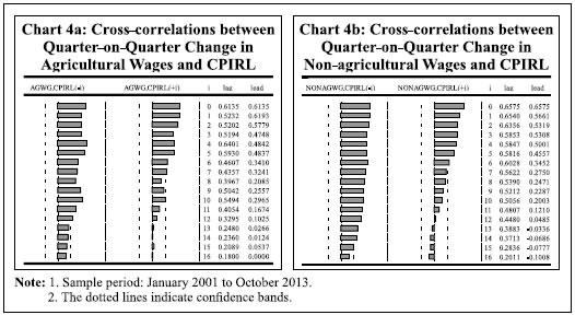 The unit root tests indicate that the variables – log of agricultural wage, log of mason wage and log of CPI-RL – were non-stationary in levels and stationary in first differences, meaning that the variables are I(1) (Appendix Table A.3). Before going to the VECM analysis, pair-wise Granger causality tests were carried out to check for the existence of bi-directional causality between the variables. The results showed the existence of a bi-directional causality between changes in rural wages and prices from January 2001 to October 2013 (which is the old series) (Appendix Table A.4a). However, the results were not the same for the new wage series, i.e., from November 2013 to February 2019 (Appendix Table A.4b). It may be mentioned that the Granger causality test has certain limitations, such as the results are not conditional upon the behaviour of other variables which might impact the relationship. Furthermore, results are also highly dependent on the sample period under consideration. Therefore, we checked for the existence of any cointegrating long-run relationship between the variables using Johansen cointegration test. The lag length was selected based on the Hannan-Quinn Information Criterion. The results of the tests indicate the presence of one cointegrating vector in both the cases, i.e., the relationship between nominal agricultural wage and price; and the relationship between nominal non-agricultural (mason) wage and price (Appendix Tables A.5 and A.6). The model specification and estimated results, both for the cointegrating equations and the error correction equations, are given in Tables 3 and 4. The agricultural sector in India continues to be heavily dependent on monsoon. | Table 3: Results of the Vector Error Correction Model between Agricultural Wage and CPI-RL | | Variables | Without Exogenous Variables | With Exogenous Variables | | D(LAGWG) | D(LCPI-RL) | D(LAGWG) | D(LCPI-RL) | | 1 | 2 | 3 | 4 | 5 | | Error Correction Term | -0.034*** | -0.006** | -0.042*** | 0.003 | | | (0.004) | (0.003) | (0.008) | (0.005) | | D(LAGWG(-1)) | -0.158** | 0.099** | -0.151* | 0.099** | | | (0.079) | (0.050) | (0.079) | (0.049) | | D(LCPI-RL(-1)) | -0.016 | 0.344*** | -0.013 | 0.331*** | | | (0.125) | (0.079) | (0.126) | (0.078) | | Constant | 0.010*** | 0.003*** | 0.011*** | 0.001 | | | (0.001) | (0.0007) | (0.002) | (0.001) | | MGNREGS dummy | - | - | -0.001 | 0.003** | | | | | (0.002) | (0.001) | | Rainfall departure from LPA | - | - | 0.000 | 0.000 | | | | | (0.000) | (0.000) | | Observations | 152 | 152 | 152 | 152 | | Adj. R-squared | 0.35 | 0.30 | 0.35 | 0.32 | | Sample period: January 2001 to October 2013. | | Long-run Association between Agricultural Wage and CPI-RL | | Without Exogenous Variables | Agricultural Wage = -7.32 + 1.94***CPI-RL
(0.074) | | With Exogenous Variables | Agricultural Wage = -6.92 + 1.87***CPI-RL
(0.081) | ***, ** & *: Represent significance at 1 per cent, 5 per cent and 10 per cent levels of significance, respectively.
Note: Figures in parentheses indicate standard errors. | Rainfall deviations from normal not only affect agricultural output but also the demand for both agricultural and non-agricultural labourers. Therefore, rainfall departure from the long period average (LPA) was included as an exogenous variable in the model. Further, the implementation of MGNREGS since February 2006 is an important policy measure of the government, having implications on the rural labour market and for rural wage setting. Therefore, a dummy variable for MGNREGS was included as an exogenous variable in the model. The dummy variable takes the value of 0 for pre-MGNREGS months, and 1 for post-MGNREGS months. | Table 4: Results of the Vector Error Correction Model between Non-agricultural Wage and CPI-RL | | Variables | Without Exogenous Variables | With Exogenous Variables | | D(LMASONWG) | D(LCPI-RL) | D(LMASONWG) | D(LCPI-RL) | | 1 | 2 | 3 | 4 | 5 | | Error Correction Term | -0.020*** | -0.008*** | -0.023*** | -0.002 | | | (0.002) | (0.003) | (0.003) | (0.005) | | D(LMASONWG(-1)) | 0.038 | -0.048 | 0.036 | -0.024 | | | (0.081) | (0.120) | (0.082) | (0.120) | | D(LCPI-RL(-1)) | 0.023 | 0.330*** | 0.023 | 0.314*** | | | (0.053) | (0.079) | (0.054) | (0.079) | | Constant | 0.007*** | 0.004*** | 0.007*** | 0.003* | | | (0.001) | (0.001) | (0.001) | (0.001) | | MGNREGS dummy | - | - | -0.001 | 0.003** | | | | | (0.001) | (0.001) | | Rainfall departure from LPA | - | - | 0.000 | 0.000 | | | | | (0.000) | (0.000) | | Observations | 152 | 152 | 152 | 152 | | Adj. R-squared | 0.69 | 0.29 | 0.68 | 0.30 | | Sample period: January 2001 to October 2013. | | Long-run Association between Non-agricultural Wage and CPI-RL | | Without Exogenous Variables | Non-agricultural Wage = -6.48 + 1.90***CPI-RL
(0.076) | | With Exogenous Variables | Non-agricultural Wage = -6.12 + 1.84***CPI-RL
(0.076) | ***, ** & *: Represent significance at 1 per cent, 5 per cent and 10 per cent levels of significance, respectively.
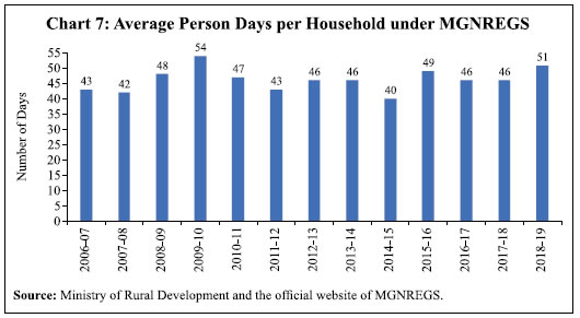
Note: Figures in parentheses indicate standard errors. | The results of the VECM analysis show that in the long-run both nominal agricultural wage and non-agricultural wage exhibit statistically significant positive relationship with price. Controlling for MGNREGS and rainfall deviations, the coefficients still remain statistically significant, though there is a marginal decline in their magnitudes (Tables 3 and 4). While the magnitudes of the long-run coefficients indicate more than full indexation of rural wages to prices, the possibility of sample bias cannot be ruled out as the average growth in nominal wages during the period under consideration was much higher than inflation. Nonetheless, the results are in conformity with the available literature (Ravallion, 2000). Furthermore, the long-run relationship between wages and prices holds given the statistically significant negative error correction terms. Any disturbance in the long-run relationship gets corrected as evident by the error correction terms in the short-run equations. However, the correction is not very quick as the magnitudes of the coefficients are small. The study could not establish the impact of prices on wages in the short-run. However, there exists a short-run relationship between agricultural wages and prices (wage impacting price) as indicated by the statistically significant coefficient of agricultural wages on prices in Table 3. The results also indicate the stickiness in nominal wages.11 The VECM equation estimated for CPI-RL, however, indicates that in the short-run changes in agricultural wages cause changes in prices (a similar result was obtained by the cross-correlation coefficients earlier), but the impact could be quite small as suggested by the magnitude of the coefficient. Interestingly, the MGNREGS dummy turns out to be statistically significant with the expected sign, although of a small magnitude, in the short-run price equations. This indicates that the implementation of MGNREGS had a positive impact on rural prices in the short-run, which could be through the demand shock as the employment under MGNREGS provides a government guaranteed wage to the rural labourers. The error correction terms for the price equations under VECM cease to appear statistically significant when exogenous variables are introduced in the model, which implies that prices may not adjust to wages in the short-run owing to several other factors that are at play. The cross-correlation coefficients discussed earlier in the paper also indicated that changes in prices lead changes in wages and not the other way round. Serial correlation tests (VEC Residual Portmanteau Tests for Autocorrelations in Appendix Tables A.7a and A.7b; VEC Residual Serial Correlation LM Tests in Appendix Tables A.8a and A.8b) and model stability tests (CUSUM tests in Charts A.1 and A.2) showed that the models are robust. Rural Wage Growth during Phase III: What Explains the Decline? This section examines the role of inflation in the recent decline in rural wage growth, i.e., post 2012–13. This period was marked by episodes of marginal uptick in wage growth, with a spell of negative growth in real wages (Charts 2 and 3). One could identify a mix of events happening during this phase, not only on the domestic front but also globally, most of which began around 2013-14, viz., the global slowdown in growth and the collapse of international commodity prices (Chart 5). 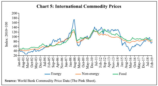 Domestically, the economy suffered two consecutive droughts in 2014-15 and 2015-16. As a result, growth in agricultural GDP turned weak. The construction sector, which grew at a fast pace during 2000-12 and was the major driver of rural non-farm employment during this period, slowed down significantly (Chart 6). These factors, along with the moderation in domestic inflation, could have suppressed rural wage growth. The employment under MGNREGS was relatively lower during this period as compared with 2008-09 to 2011-12 (Chart 7). 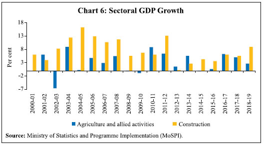
 The empirical exercise to examine the factors behind the recent slowdown in rural wage growth was undertaken using data for the period November 2013 to February 2019. The wage-price relationship was also examined for this phase, after controlling for factors like MGNREGS, construction sector slackness and rainfall deviations from normal.12 Furthermore, the analysis was undertaken using state-level data to ensure that the sample reflects all the variabilities in the variables. A dynamic panel data analysis with the Arellano–Bover/Blundell–Bond system GMM structure was the most appropriate econometric technique available for this part of the study.13 The explanatory variables were chosen as per the events discussed above. The MGNREGS wage reflects some sort of a proxy for minimum wage or a government guaranteed base price for rural labour. The MGNREGS wages and rural wages are expected to be positively related. One could also expect rural agricultural wages to be positively related with construction wages, as a higher wage in the construction sector would attract unskilled labourers from agriculture, which could then drive agricultural wages up by creating a shortage of agricultural labourers. While we do not have output/unemployment rate as an explanatory variable in the model due to data limitations, construction wage could also represent, albeit in a limited manner, the overall health of the economy (equation (2) in section II of the paper). Furthermore, the rainfall deviation from normal level (LPA) would affect agricultural output as well as the demand for both agricultural and non-agricultural labourers. Greater the deviation of rainfall from normal, lower would be the wage. Apart from the demand aspect, we expect rainfall deviations to also reflect the associated change in agricultural productivity. Nevertheless, the literature suggests that the impact of agricultural productivity on rural wage variations has declined over the years (Himanshu and Kundu, 2016). All variables were converted to their natural logarithms. Data for state-wise MGNREGS wage were collected from the Ministry of Rural Development and the official website of MGNREGS. Arellano–Bond tests for zero autocorrelation in first-differenced errors confirmed the robustness of the models. The results of the regression analysis show that from November 2013 to February 2019 (new wage series) changes in rural prices had a positive and significant impact on changes in nominal agricultural wages in a contemporaneous manner (Tables 5a and 5b). The regression equations in Table 5a include CPI-RL as the measure of rural prices, while those in Table 5b include the all-India CPI-Rural index. The availability of new all-India CPI-Rural index (base 2012=100) from January 2011 allowed us to look at the impact of change in all India rural prices on agricultural wages, which was not possible with the use of CPI-RL due to its sectoral representation of CPI. The coefficient of price with lag t-1 also suggests that wages take a month time to adjust to changes in prices. This means that the next period’s real wage will not show a complete adjustment, even when the inflationary/deflationary shock is over. The results also show a positive and statistically significant impact of construction wages on agricultural wages and their impact is realised even with a lag of two months as indicated by the coefficient of construction wage with two months lag, which implies that not only the current period construction wage has a positive impact on agricultural wage, but construction wage with a two-period lag also impacts agricultural wages positively. This establishes the role of rural non-farm sector in driving agricultural wages. Unlike in the past, MGNREGS did not create a significant impact on agricultural wages during this period, with its coefficients not being statistically significant (when CPI-Rural index is used). | Table 5a: Results of the Dynamic Panel Data Models | | Dependent variable: Agricultural wage | | Model | I | II | III | | Explanatory Variables | Coefficient | Z value | Coefficient | Z value | Coefficient | Z value | | 1 | 2 | 3 | 4 | 5 | 4 | 5 | | Agricultural wage (t-1) | 0.21 | 3.12*** | 0.21 | 3.50*** | 0.22 | 3.74*** | | Agricultural wage (t-2) | -0.07 | -0.79 | -0.06 | -0.63 | -0.09 | -0.85 | | MGNREGS wage | 0.16 | 2.40** | 0.16 | 2.38** | 0.16 | 2.38** | | MGNREGS wage (t-1) | -0.01 | -0.22 | -0.01 | -0.31 | -0.005 | -0.10 | | MGNREGS wage (t-2) | -0.04 | -0.74 | -0.03 | -0.56 | -0.04 | -0.63 | | CPI-RL | 0.31 | 3.33*** | 0.31 | 3.29*** | 0.29 | 3.29*** | | CPI-RL (t-1) | -0.16 | -1.92* | -0.14 | -1.70* | -0.15 | -1.60 | | CPI-RL (t-2) | 0.11 | 0.79 | 0.08 | 0.55 | 0.09 | 0.71 | | Construction Wage | 0.74 | 9.44*** | 0.74 | 9.29*** | 0.75 | 9.85*** | | Construction Wage (t-1) | -0.13 | -1.80* | -0.13 | -1.94* | -0.15 | -1.99** | | Construction Wage (t-2) | 0.15 | 1.85* | 0.14 | 1.70* | 0.17 | 1.80* | | Rainfall Departure | -0.003 | -1.65* | -0.003 | -1.89* | -0.002 | -1.36 | | Rainfall Departure (t-4) | - | - | -0.0004 | -0.40 | - | - | | Rainfall Departure (t-12) | - | - | - | - | -0.003 | -1.70* | | Constant | -1.76 | -3.06*** | -1.74 | -2.99*** | -1.67 | -2.78*** | | Arellano–Bond test for zero autocorrelation in first differenced errors (Order 2)# | Z = 0.45
[0.65] | Z = 0.27
[0.79] | Z = 0.32
[0.75] | | Wald chi2(12;13;13) | 2297.44***
[0.00] | 2753.81***
[0.00] | 2259.26***
[0.00] | | No. of observations | 1170 | 1125 | 976 | ***, ** & *: Represent significance at 1 per cent, 5 per cent and 10 per cent levels of significance, respectively; #: The null hypothesis is no autocorrelation.
Note: 1. Figures in [ ] indicate probability.
2. Sargan test of overidentifying restrictions (Null Hypothesis: Overidentifying restrictions are valid) results for models I, II and III are: chi2 (1304) = 1421.06 [Prob. value = 0.01], chi2 (1279) = 1453.03 [Prob. value = 0.00] and chi2 (1140) = 1240.41 [Prob. value = 0.02], respectively. The distribution of the Sargan test is known only when the errors are independently and identically distributed. For this reason, the Sargan test does not produce a test statistic when robust standard errors are obtained in this model. The coefficients reported in the table correspond to robust standard errors. Therefore, the Sargan test results were obtained by specifying the model without the command for robust standard errors. The coefficients remained almost unchanged under both the models. We attribute the rejection of the null hypothesis under Sargan test, wherever applicable, to the possible presence of heteroscedasticity in the data generating process, thus, requiring to go for a robust standard error model (Arellano and Bond, 1991). |
| Table 5b: Results of the Dynamic Panel Data Models | | Dependent variable: Agricultural wage | | Model | I | II | III | | Explanatory Variables | Coefficient | Z value | Coefficient | Z value | Coefficient | Z value | | 1 | 2 | 3 | 4 | 5 | 4 | 5 | | Agricultural wage (t-1) | 0.20 | 2.88*** | 0.20 | 3.24*** | 0.21 | 3.41*** | | Agricultural wage (t-2) | -0.08 | -0.84 | -0.08 | -0.79 | -0.10 | -0.96 | | MGNREGS wage | 0.15 | 1.46 | 0.15 | 1.47 | 0.15 | 1.48 | | MGNREGS wage (t-1) | -0.04 | -0.67 | -0.04 | -0.69 | -0.03 | -0.46 | | MGNREGS wage (t-2) | -0.06 | -1.09 | -0.06 | -1.17 | -0.07 | -1.22 | | CPI-Rural | 0.28 | 2.70*** | 0.28 | 2.66*** | 0.27 | 2.83*** | | CPI-Rural (t-1) | -0.08 | -1.14 | -0.08 | -1.08 | -0.08 | -1.16 | | CPI-Rural (t-2) | 0.13 | 2.90*** | 0.13 | 2.79*** | 0.13 | 2.80*** | | Construction Wage | 0.75 | 10.46*** | 0.75 | 10.36*** | 0.76 | 10.97*** | | Construction Wage (t-1) | -0.11 | -1.58 | -0.12 | -1.69* | -0.14 | -1.78* | | Construction Wage (t-2) | 0.18 | 2.11** | 0.17 | 2.04** | 0.20 | 2.07** | | Rainfall Departure | -0.003 | -1.58 | -0.003 | -1.89* | -0.002 | -1.35 | | Rainfall Departure (t-4) | - | - | 0.001 | 0.42 | - | - | | Rainfall Departure (t-12) | - | - | - | - | -0.003 | -1.49 | | Constant | -1.54 | -3.25*** | -1.56 | -3.30*** | -1.45 | -3.25*** | | Arellano–Bond test for zero autocorrelation in first differenced errors (Order 2)# | Z = 0.56
[0.57] | Z = 0.49
[0.62] | Z = 0.58
[0.56] | | Wald chi2(12;13;13) | 1736.42***
[0.00] | 2045.44***
[0.00] | 1971.06***
[0.00] | | No. of observations | 1170 | 1125 | 976 | ***, ** & *: Represent significance at 1 per cent, 5 per cent and 10 per cent levels of significance, respectively; #: The null hypothesis is no autocorrelation.
Note: 1. Figures in [ ] indicate probability.
2. Sargan test of overidentifying restrictions (Null Hypothesis: Overidentifying restrictions are valid) results for models I, II and III are: chi2 (1304) = 1371.04 [Prob. value = 0.10], chi2 (1279) = 1395.67 [Prob. value = 0.01] and chi2 (1140) = 1197.89 [Prob. value = 0.11], respectively. Please see note 2 to table 5a. | Section VI Conclusion The main objective of the paper is to study the relationship between rural wage growth and inflation over the past 15 years and examine the risk of a wage-price spiral to the inflation trajectory in India. Another objective of the paper is to identify the factors responsible for the recent slowdown in agricultural wage growth. The short-run and long-run dynamics of changes in rural wages and prices were examined by studying the lead-lag relationships using cross-correlation coefficients. The paper also applied cointegration and VECM methods to analyse short-run and long-run dynamics between wages and prices. To ascertain the determinants of the deceleration in agricultural wage growth in recent years the paper used a dynamic panel data model with the Arellano–Bover/Blundell–Bond system GMM structure. The results exhibited that, in the long-run, both nominal agricultural wages and non-agricultural wages have statistically significant positive relationship with prices. The results of the panel regression analysis showed that from November 2013 to February 2019, rural prices had a positive and significant contemporaneous impact on nominal agricultural wages. Nominal wages also displayed stickiness in the short-run. Proxied by construction sector wage, the rural non-farm sector wages demonstrated a positive and statistically significant relationship with the agricultural wage growth, indicating the role of rural non-farm sector wage behaviour in influencing agricultural wages. In terms of policy implications, weaker evidence on wage-push induced risks to the inflation trajectory and stronger evidence of inflation induced wage pressures suggest limited risk of a wage-price spiral to the price stability goal under the flexible inflation targeting framework in India.
References Abraham, V. (2009). “Employment growth in rural India: Distress-driven?”, Economic and Political Weekly, 44(16): 97–104. Arellano, M., and Bond, S. (1991). “Some tests of specification for panel data: Monte Carlo evidence and an application to employment equations”, Review of Economic Studies, 58, 277-297. Bank for International Settlements (BIS) (2017), 87th Annual Report, 1 April–31 March 2017, Basel, 25 June, available at: https://www.bis.org/publ/arpdf/ar2017e.pdf. Bardhan, P. (1970). “‘Green Revolution’ and agricultural labourers”, Economic and Political Weekly, 5(2), 1239–46. Rao, V. M. (1987). “Land, labour and rural poverty: Essays in development economics by Bardhan, Pranab K.”, Book Review, Indian Journal of Agricultural Economics, 42(2), 221. Berg, E., Bhattacharyya, S., Durgam, R., and Ramachandra, M. (2012). “Can rural public works affect agricultural wages? Evidence from India”, CSAE Working Paper, WPS/2012-05. Bhalla, S. (1979). “Real wage rates of agricultural labourers in Punjab, 1961–77: A preliminary analysis”, Economic and Political Weekly, 14(26), A57-A68. Blackburne III, E. F., and Frank, M. W. (2007). “Estimation of nonstationary heterogeneous panels”, The Stata Journal, 7(2), 197–208. Blanchard, O. (1998). “The Wage Equation”, Lecture Notes, MIT. Boyce, J., and Ravallion, M. (1991). “A dynamic econometric model of agricultural wage determination in Bangladesh”, Oxford Bulletin of Economics and Statistics, 53(4), 361–76. Braumann, B. (2001). “High Inflation and Real Wages”, IMF Staff Papers, 51(1), 123–47. Braumann, B., and Shah, S. (1999). “Suriname: A case study of high inflation”, IMF Working Paper, No. 99/157, International Monetary Fund. Chand, R., Garg, S., and Pandey, L. (2009). “Regional variations in agricultural productivity: A district level study”, Discussion Paper NPP 01/2009, National Professor Project, National Centre for Agricultural Economics and Policy Research, Indian Council of Agricultural Research, New Delhi. Chand, R., Srivastava, S. K., and Singh, J. (2017). “Changing structure of rural economy of India: Implications for employment and growth”, NITI AAYOG Discussion Paper, Niti Aayog, pp. 1–30. Das, A., and Usami, Y. (2017). “Wage rates in rural India, 1998–99 to 2016–17”, Review of Agrarian Studies, 7(2), 4–38. Datt, G., and Ravallion, M. (1998). “Farm productivity and rural poverty in India”, The Journal of Development Studies, 34(4), 62–85. Deaton, A., and Dreze, J. (2002). “Poverty and inequality in India: A re-examination”, Economic and Political Weekly, 37(36), 3729–48. Dornbusch, R., and Edwards, S. (eds.). (1992). The macroeconomics of populism in Latin America, Chicago and London: University of Chicago Press. Goyal, A., and Baikar, A. K. (2014). “Psychology, cyclicality or social programs: Rural wage and inflation dynamics in India”. Guha, A., and Tripathi, A. K. (2014). “Link between food price inflation and rural wage dynamics”, Economic and Political Weekly, 49(26), 66–73. Gulati, A., and Saini, S. (2013). “Taming food inflation in India”, Commission for Agricultural Costs and Prices Discussion Paper, 4. Himanshu. (2005). “Wages in rural India: Sources, trends and comparability”, Indian Journal of Labour Economics, 48(2), 375–406. ______ (2006). “Agrarian crisis and wage labour: A regional perspective”, Indian Journal of Labour Economics, 49(4), 827–46. Himanshu, Lanjouw, P., Murgai, R., and Stern, N. (2013). “Nonfarm diversification, poverty, economic mobility, and income inequality: A case study in village India”, Agricultural Economics, 44(4–5), 461–73. Himanshu., and Kundu, S. (2016). “Rural wages in India: Recent trends and determinants”, The Indian Journal of Labour Economics, 59(2), 217–44. Imbert, C., and Papp, J. (2015). “Labor market effects of social programs: Evidence from India’s employment guarantee”, American Economic Journal: Applied Economics, 7(2), 233–63. Jacoby, H. G. (2015). “Food prices, wages, and welfare in rural India (English)”, Economic Inquiry, 18 June. Jose, A. V. (1974). “Trends in real wage rates of agricultural labourers”, Economic and Political Weekly, 9(13), A25–A30. Kessel, R. A., and Alchian, A. A. (1960). “The meaning and validity of the inflation-induced lag of wages behind prices”, The American Economic Review, 50(1), 43–66. Knotek II, E. S., and Zaman, S. (2014). “On the relationships between wages, prices, and economic activity”, Economic Commentary, Federal Reserve Bank of Cleveland, August issue. Lal, D. (1976). “Agricultural growth, real wages, and the rural poor in India”, Economic and Political Weekly, 11(26), A47–A61. Nadhanael, G. V. (2012). “Recent trends in rural wages: An analysis of inflationary implications”, Reserve Bank of India Occasional Papers, 33(1), 89–112. Pandey, L. (2012). “Effects of price increase and wage rise on resource diversification in agriculture: The case of Uttar Pradesh”, Economic and Political Weekly, 47(26/27), 100–05. Radhakrishna, R., and Chandrasekhar, S. (2008). “Overview: Growth: Achievements and Distress”. In R. Radhakrisnan (eds.), India Development Report, Oxford University Press. Ravallion, M. (2000). “Prices, wages and poverty in rural India: What lessons do the time series data hold for policy?”, Food Policy, 25(3), 351–64. Reserve Bank of India (RBI). 2012. Reserve Bank of India Annual Report 2011–12, Reserve Bank of India, Mumbai. Roodman, D. (2009). “How to do xtabond2: An introduction to difference and system GMM in Stata”, The Stata Journal, 9(1), 86–136. Sen, A. (1996). “Economic reforms, employment and poverty: Trends and options”, Economic and Political Weekly, 31(35/37), 2459–77. Tyagi, D. S. (1979). “Farm Prices and Class Bias in India”, Economic and Political Weekly, 14(39), A111–A124. Vakulabharanam, V. (2005). “Growth and distress in a South Indian peasant economy during the era of economic liberalisation”, The Journal of Development Studies, 41(6), 971–97. Venkatesh, P. (2013). “Recent trends in rural employment and wages in India: Has the growth benefitted the agricultural labours?”, Agricultural Economics Research Review, 26(347-2016-17099), 13–20.
Appendix | Table A.1: Test Results for Statistical Break in year-on-year Growth in Agricultural Wage | | Quandt-Andrews Unknown Breakpoint Test14 | | Statistic | Value | Prob. | | Maximum LR F-Statistic (2014 M11) | 47.241 | 0.000*** | | Maximum Wald F-Statistic (2014 M11) | 94.482 | 0.000*** | | Exp LR F-Statistic | 18.479 | 0.000*** | | Exp Wald F-Statistic | 42.099 | 0.000*** | | Ave LR F-Statistic | 1.573 | 0.141 | | Ave Wald F-Statistic | 3.146 | 0.141 | | Period: January 2002 to November 2017. | ***, ** & *: Represent significance at 1 per cent, 5 per cent and 10 per cent levels of significance, respectively.
Note: Probabilities calculated using Hansen’s (1997) method. |
| Table A.2: Test Results for Statistical Break in Year-on-Year Growth in Non-agricultural Wage | | Quandt-Andrews Unknown Breakpoint Test15 | | Statistic | Value | Prob. | | Maximum LR F-Statistic (2014 M11) | 24.954 | 0.000*** | | Maximum Wald F-Statistic (2014 M11) | 49.908 | 0.000*** | | Exp LR F-Statistic | 7.352 | 0.000*** | | Exp Wald F-Statistic | 19.813 | 0.000*** | | Ave LR F-Statistic | 2.080 | 0.057 | | Ave Wald F-Statistic | 4.160 | 0.057 | | Period: January 2002 to November 2017. | ***, ** & *: Represent significance at 1 per cent, 5 per cent and 10 per cent levels of significance, respectively.
Note: Probabilities calculated using Hansen’s (1997) method. |
| Table A.3: Unit Root Test Results (Phillips–Perron Test)16 | | | LAGWG | D(LAGWG) | LMASONWG | D(LMASONWG) | LCPI-RL | D(LCPI-RL) | | Adj. t-Statistic | 7.326 | -7.392*** | 6.931 | -2.323** | 8.376 | -3.757*** | | P-value# | 1.000 | 0.000 | 1.000 | 0.020 | 1.000 | 0.000 | | Sample Period: January 2001 to October 2013. | ***, ** & *: Represent significance at 1 per cent, 5 per cent and 10 per cent levels of significance, respectively.
Note: #MacKinnon (1996) one-sided p-values. |
| Table A.4a: Pair-wise Granger Causality Test Results | | Null Hypothesis | Obs. | F-Statistic | Prob. | | D(CPI-RL) does not Granger Cause D(AGWG) | 151 | 2.95 | 0.06* | | D(AGWG) does not Granger Cause D(CPI-RL) | 151 | 7.50 | 0.00*** | | D(CPI-RL) does not Granger Cause D(MASONWG) | 151 | 2.90 | 0.06* | | D(MASONWG) does not Granger Cause D(CPI-RL) | 151 | 12.63 | 0.01*** | | Sample Period: January 2001 to October 2013. | | ***, ** & *: Represent significance at 1 per cent, 5 per cent and 10 per cent levels of significance, respectively. |
| Table A.4b: Pair-wise Granger Causality Test Results | | Null Hypothesis | Obs. | F-Statistic | Prob. | | D(CPI-RL) does not Granger Cause D(AGWG) | 61 | 2.72 | 0.07* | | D(AGWG) does not Granger Cause D(CPI-RL) | 61 | 0.61 | 0.55 | | D(CPI-RL) does not Granger Cause D(MASONWG) | 61 | 0.85 | 0.43 | | D(MASONWG) does not Granger Cause D(CPI-RL) | 61 | 0.96 | 0.39 | | Sample Period: November 2013 to February 2019. | | ***, ** & *: Represent significance at 1 per cent, 5 per cent and 10 per cent levels of significance, respectively. |
| Table A.5: Results of the Cointegration Tests between Agricultural Wage and CPI-RL | | Series: LAGWG LCPI-RL | | Unrestricted Cointegration Rank Test (Trace) | | Hypothesized No. of CE(s) | Eigenvalue | Trace Statistic | 0.05 Critical Value | Prob.$ | | None# | 0.163 | 27.883 | 15.495 | 0.000 | | At most 1 | 0.007 | 1.030 | 3.841 | 0.310 | | Unrestricted Cointegration Rank Test (Maximum Eigenvalue) | | Hypothesized No. of CE(s) | Eigenvalue | Max-Eigen Statistic | 0.05 Critical Value | Prob.$ | | None# | 0.163 | 26.853 | 14.265 | 0.000 | | At most 1 | 0.007 | 1.030 | 3.841 | 0.310 | | Sample period: January 2001 to October 2013; | | Sample period (adjusted): April 2001 to October 2013. | | Observations: 151 after adjustments. | #: Denotes rejection of the hypothesis at the 0.05 level; $: Denotes MacKinnon-Haug-Michelis (1999) p-values.
Note: Both Trace and Max Eigen value tests indicate the presence of one cointegrating vector. |
| Table A.6: Results of the Cointegration Tests between Non-agricultural Wage and CPI-RL | | Series: LMASONWG LCPI-RL | | Unrestricted Cointegration Rank Test (Trace) | | Hypothesized No. of CE(s) | Eigenvalue | Trace Statistic | 0.05 Critical Value | Prob.$ | | None# | 0.255 | 45.970 | 15.495 | 0.000 | | At most 1 | 0.008 | 1.191 | 3.841 | 0.275 | | Unrestricted Cointegration Rank Test (Maximum Eigenvalue) | | Hypothesized No. of CE(s) | Eigenvalue | Max-Eigen Statistic | 0.05 Critical Value | Prob.$ | | None# | 0.255 | 44.779 | 14.265 | 0.000 | | At most 1 | 0.008 | 1.030 | 3.841 | 0.275 | | Sample period: January 2001 to October 2013; | | Sample period (adjusted): March 2001 to October 2013. | | Observations: 152 after adjustments. | #: Denotes rejection of the hypothesis at the 0.05 level; $: MacKinnon-Haug-Michelis (1999) p-values.
Note: Both Trace and Max Eigen value tests indicate the presence of one cointegrating vector. |
| Table A.7a: VEC Residual Portmanteau Tests for Autocorrelations | | Series: LAGWG LCPI-RL | | Null Hypothesis: No residual autocorrelations up to lag h. | | Lags | Q-Stat | Prob.* | Adj Q-Stat | Prob.* | df | | 1 | 0.51 | - | 0.51 | - | - | | 2 | 6.26 | 0.39 | 6.34 | 0.39 | 6 | | Sample period: January 2001 to October 2013. | | Observations: 152 after adjustments. | *: df and Prob. may not be valid for models with exogenous variables.
Note: 1. Test is valid only for lags larger than the VAR lag order.
2. df is degrees of freedom for (approximate) chi-square distribution after adjustment for VEC estimation (Bruggemann, et al., 2005). |
| Table A.7b: VEC Residual Portmanteau Tests for Autocorrelations | | Series: LMASONWG LCPI-RL | | Null Hypothesis: No residual autocorrelations up to lag h. | | Lags | Q-Stat | Prob.* | Adj Q-Stat | Prob.* | df | | 1 | 0.46 | - | 0.47 | - | - | | 2 | 4.86 | 0.56 | 4.92 | 0.55 | 6 | | Sample period: January 2001 to October 2013. | | Observations: 152 after adjustments. | *: df and Prob. may not be valid for models with exogenous variables.
Note: 1. Test is valid only for lags larger than the VAR lag order.
2. df is degrees of freedom for (approximate) chi-square distribution after adjustment for VEC estimation (Bruggemann, et al., 2005). |
| Table A.8a: VEC Residual Serial Correlation LM Tests | | Series: LAGWG LCPI-RL | | Null Hypothesis: No serial correlation at lag h. | | Lags | LRE* Stat | df | Prob. | Rao F-Stat | df | Prob. | | 1 | 0.51 | 4 | 0.25 | 1.36 | (4,286.0) | 0.25 | | 2 | 6.26 | 4 | 0.20 | 1.51 | (4,286.0) | 0.20 | | Null Hypothesis: No serial correlation at lags 1 to h. | | Lags | LRE* Stat | df | Prob. | Rao F-Stat | df | Prob. | | 1 | 5.43 | 4 | 0.27 | 1.36 | (4,286.0) | 0.25 | | 2 | 7.03 | 8 | 0.53 | 0.88 | (8,282.0) | 0.53 | | Sample period: January 2001 to October 2013. | | Observations: 152 after adjustments. | | *: Denotes Edgeworth expansion corrected likelihood ratio statistic. |
| Table A.8b: VEC Residual Serial Correlation LM Tests | | Series: LMASONWG LCPI-RL | | Null Hypothesis: No serial correlation at lag h. | | Lags | LRE* Stat | df | Prob. | Rao F-Stat | df | Prob. | | 1 | 8.41 | 4 | 0.08 | 2.13 | (4,286.0) | 0.08 | | 2 | 4.45 | 4 | 0.35 | 1.12 | (4,286.0) | 0.35 | | Null Hypothesis: No serial correlation at lags 1 to h. | | Lags | LRE* Stat | df | Prob. | Rao F-Stat | df | Prob. | | 1 | 8.41 | 4 | 0.08 | 2.13 | (4,286.0) | 0.08 | | 2 | 9.45 | 8 | 0.31 | 1.19 | (8,282.0) | 0.31 | | Sample period: January 2001 to October 2013. | | Observations: 152 after adjustments. | | *: Denotes Edgeworth expansion corrected likelihood ratio statistic. |
|