Dirghau Keshao Raut and Swati Raju* A rule-based fiscal regime, through the enactment of Fiscal Responsibility Legislations (FRLs), was adopted by state governments against the backdrop of growing debt and deficits in the early 2000s. Literature has documented the positive impact of fiscal rules in terms of fiscal discipline. However, the evidence with regard to cyclicality of fiscal policy is mixed. This paper examines the impact of fiscal rules on the cyclicality of fiscal policy of Indian states using data for the period from 1990 to 2018. The results suggest that fiscal rules have reduced pro-cyclicality of fiscal policy, particularly in terms of development expenditure. Fiscal deficit also changed its nature from pro-cyclical in the pre-FRL period to acyclical in the post-FRL period. Capital outlay displayed acyclical behaviour in both pre-and post-FRL periods. JEL Classification: E62, C23, H62, H72 Keywords: Fiscal policy, states’ expenditure, cyclicality Introduction Cross-country practices at national and sub-national levels suggest that fiscal rules have been adopted to discipline fiscal policy and to maintain fiscal sustainability (Grembi et al., 2016; Guerguil et al., 2016; IMF, 2017). In the context of Indian states, rising level of debt and deficits during the late 1990s and early 2000s necessitated the implementation of fiscal reforms at the state level and a major step in this direction was the adoption of Fiscal Responsibility Legislations (FRLs) incentivised by the Twelfth Finance Commission (Finance Commission, 2004). Several studies in the cross-country as well as in the Indian context have established the contribution of fiscal rules to achieve fiscal consolidation (Alesina and Bayoumi, 1996; Chakraborty and Dash, 2017; GoI, 2017; Marneffe et al., 2010; Simone and Topalova 2009; Tapsoba, 2012). There have, however, been concerns about fiscal policy being pro-cyclical in a rule-based fiscal regime due to restrictions on borrowings. Cyclicality of fiscal policy refers to the direction of change in government expenditure and taxes relative to economic/output conditions. The fiscal policy is considered pro-cyclical, if it is expansionary during economic booms and contractionary during recessions. On the other hand, if fiscal policy is expansionary during recessions and contractionary during booms, it is considered to be counter-cyclical. Keynes advocated a counter-cyclical fiscal policy – running a budgetary deficit during slowdown. In contrast, balanced budget rules generally produce a pro-cyclical fiscal policy. Decline in revenues during an economic slowdown enforces reduction in expenditure, while buoyant revenues during a high economic growth phase allow for increase in expenditure leading to a pro-cyclical fiscal policy. Clemens and Miran (2012) argue that balanced budget requirements lead to compressed government expenditures due to contraction in tax base during recession periods. Fatas and Mihov (2006) observe that restrictions on fiscal policy impair a government’s ability to run a counter-cyclical fiscal policy. Bova et al. (2014) find fiscal policy under fiscal rules to be pro-cyclical and argue that cyclically adjusted targets and escape clauses may reduce pro-cyclicality. There are, however, studies arguing that fiscal rules help in generating fiscal space which leads to lesser pro-cyclical or a counter-cyclical fiscal policy. For example, Nerlich and Reuter (2015) find an evidence of fiscal rules linked with higher fiscal space. They argue that fiscal discipline reduces deficits and debt, thus, widening the gap between debt limit and actual debt leading to increase in fiscal space. They also find evidence of higher fiscal space contributing to higher discretionary expenditure. Aizenman et al. (2019) observe that public expenditure by a government with lower fiscal space (high debt level) tends to be more pro-cyclical than that by a government having more fiscal space (low debt level). Simone and Topalova (2009) argue that fiscal consolidation creates fiscal space for following a counter-cyclical fiscal policy. Manasse (2005) finds that the impact of fiscal rules on cyclicality varies during different economic conditions. The restrictions on deficits are found to be associated with counter-cyclical policies during ‘very good’ or ‘very bad’ economic conditions, and with pro-cyclical policies during the intermediate state of the economy. The design of fiscal rules is also documented to have an impact on cyclicality. For example, cyclically adjusted budget balance rules are associated with counter-cyclical public spending (Guerguil et al., 2016; Misra and Ranjan, 2019). Guerguil et al. (2016) observe a reduction in pro-cyclicality of investment spending when rules are investment-friendly. In the case of Indian states, there is limited literature on the impact of fiscal rules on the cyclicality of fiscal policy. This paper thus seeks to fill this gap and examines the role of fiscal rules in influencing the nature of cyclicality of states’ fiscal policy in terms of development expenditure, capital outlay and fiscal deficit. Section II presents a review of relevant literature. Section III describes major features of the FRLs of states and the progress with respect to fiscal consolidation. Methodology is discussed in Section IV and empirical results are presented in Section V. Section VI concludes the paper. Section II
Review of the Literature While several country-specific as well as cross-country studies examined the various aspects of fiscal rules, this section focuses on studies analysing the impact of fiscal rules on cyclicality of revenues/expenditure and fiscal consolidation. Most of the studies have found fiscal rules contributing to fiscal consolidation, though the evidence on cyclicality of fiscal policy is mixed, i.e., pro-cyclical, counter-cyclical and acyclical. Alesina and Bayoumi (1996), using data for the period from 1965 to 1992 for 48 mainland states in the United States (US), found a positive impact of fiscal controls on budget surplus as well as higher primary surplus. Further, cyclical variability of surplus was found to be lower in states with more stringent fiscal controls. They, however, pointed out that fiscal controls did not result in any cost in terms of output variability. Based on state level data of the US from 1963 to 2000, Fatas and Mihov (2006) found that fiscal policy restrictions helped to reduce budget deficits but impaired the government’s ability to run a counter-cyclical fiscal policy. Clemens and Miran (2012) used data for 27 US states for the period 1988 to 2004 and found that balanced budget requirements caused compression in capital and other expenditures. Mcgranahan and Mattoon (2012), using quarterly data of 50 US states from 1980 to 2011, found evidence of pro-cyclical revenues, i.e., a 1 percentage point increase in the growth of coincident indicator of economic conditions leading to a 0.9 percentage point increase in revenues. Cross-country studies generally found evidence of pro-cyclical fiscal policy. Using data on 13 Latin American countries, Gavin and Perotti (1997) observed that economic downturns restricted the increase in government expenditure (due to higher borrowing cost) leading to a pro-cyclical fiscal policy. Estimating a weighted least square model based on annual data from 1960 to 1998 for 22 OECD countries, Lane (2003) found varying cyclicality across countries and expenditure categories. While current expenditure was found to be counter-cyclical, its consumption components were pro-cyclical. Similarly, government investment expenditure was found to be most pro-cyclical, while interest payments were found to be acyclical. Cross-country coefficients of cyclicality were, however, observed to differ across countries, i.e., the US and the United Kingdom (UK) showed counter-cyclical fiscal behaviour, whereas Ireland and Portugal showed above average pro-cyclical fiscal behaviour. In a study based on panel data for 1995-2008 pertaining to 16 countries in the euro area, Marneffe et al. (2010) found a positive association between the fiscal rule index and total and primary fiscal balance, and a negative impact of fiscal rules on government expenditure. Using data for 62 developing and industrial countries for the period 1960-2009, Vegh and Vuletin (2011) found tax policy to be pro-cyclical in developing countries and acyclical in industrial countries. They also observed government spending to be pro-cyclical in developing countries and counter-cyclical in industrial countries. However, Ilzetzki and Vegh (2008), using quarterly data of 49 countries from 1960 to 2006, observed pro-cyclical government consumption spending in developing as well as high-income countries. Using panel data of 72 countries, Cicek and Elgin (2011) found evidence of more pronounced pro-cyclicality of fiscal policy in countries with a larger size of shadow economy. They suggested strengthening of tax enforcement and improving legal and administrative processes to reduce the shadow economy and pro-cyclicality of fiscal policy. Aghion and Marinescu (2008) provided evidence of a more counter-cyclical budgetary policy with higher level of financial development, adoption of inflation targeting and lower openness of the economy. The design of fiscal rules in terms of balanced budget rule (BBR) and cyclically adjusted balance (CAB) was found to influence the cyclicality of fiscal policy. Misra and Ranjan (2019), using a correlation approach for data on 61 countries from 2001 to 2016, found a positive correlation between expenditure and gross domestic product (GDP) in 75 per cent of the sample countries. In the panel system GMM estimation, results showed higher pro-cyclicality coefficient (0.92) for a sub-sample of 25 countries with BBR vis-à-vis that for overall sample (0.66) and for sub-sample of countries with fiscal rule in terms of CAB (-0.08). Studies on fiscal rules in the context of Indian states have looked into aspects such as fiscal discipline; causes of slower/faster adoption of FRL; impact of fiscal rules on development expenditure, guarantees given by states, borrowings by state utilities; and forecasting of revenues. Simone and Topalova (2009) observed that higher transfer dependent states were slower in adopting FRLs. They also observed that the enactment of FRLs coincided with fiscal consolidation. Further, the impact on fiscal discipline was stronger when FRLs included debt target and expenditure rules. Buiter and Patel (2010), based on a review of seven major states, observed ‘discretionary counter-cyclical’ fiscal policy at the state level in India. Using data pertaining to 14 states for the period from 2000-01 to 2013-14, Chakraborty and Dash (2017) estimated the panel GMM model and found evidence of reduction in gross fiscal deficit (GFD)-gross state domestic product (GSDP) ratio and revenue deficit (RD)-GSDP ratio after the introduction of fiscal rules. The study also found that states have reduced their discretionary development expenditure to maintain the deficit targets as per their fiscal rules. The Economic Survey 2016–17 (GoI, 2017), observed that revenue deficit of states declined by 2.5 percentage points of GSDP in the post-FRL period. The survey pointed out that several factors contributed to this improvement such as increase in states’ own tax revenue due to acceleration in nominal GDP growth; increased central transfers; decline in interest payments due to debt restructuring; and the Centre’s contribution in social sector expenditure under Centrally Sponsored Schemes. The regression results showed that FRLs contributed to the decline in RD and GFD but not primary deficit. The survey also observed a decline in guarantees in the three year period post-FRLs, and a decrease in borrowings by states’ utilities and an improvement in forecasting of own tax revenues in the post-FRL years. Though not in the context of fiscal rules, studies have examined the cyclicality of expenditure by Indian states. The results are mixed and vary across expenditure components. For example, based on data for 17 non-special category states and estimating panel least square (LS), instrument variables (IV) and 2SLS estimation, Kaur et al. (2013) observed acyclical social sector expenditure (SSE) on account of downward rigidity of SSE in the revenue account, and pro-cyclical education expenditure with pro-cyclicality being more pronounced during upturns, defined as positive output gap. Using correlation analysis, pooled least square technique and 2SLS method on data for 14 states, the RBI (2014) observed the capital outlay of states to be pro-cyclical and primary revenue expenditure to be acyclical. Section III
Fiscal Rules and Fiscal Consolidation at the State Level Fiscal rules are generally implemented through legislative provisions for the conduct of fiscal policy in terms of operational targets including escape clauses for deviation from such targets. While the adoption of fiscal rules began in advanced countries, some emerging market economies and underdeveloped countries have also adopted fiscal rules regimes successfully (IMF, 2017). Though the nature of fiscal rules varies across countries, they usually include ceilings on deficit-GDP ratio, revenue balance, primary balance and debt. Revenue and expenditure targets are also sometimes used as operating targets in a rule-based fiscal policy. In some countries, implementation of fiscal rules has been advocated as a pre-condition to implement certain macroeconomic policies. In India, the Committee on Capital Account Convertibility 1997 (Chairman: Shri S. S. Tarapore) recommended the fiscal deficit of the central government at 3.5 per cent of GDP along with reduction in states’ deficit and quasi-fiscal deficit as a precondition for capital account convertibility (RBI, 1997). The fiscal rules at the state level in India were adopted in the backdrop of a prolonged deterioration in state finances and the consequent fiscal reforms. The fiscal position of states witnessed deterioration beginning late 1980s due to increased expenditure on salaries and pensions after the implementation of the Fourth Pay Commission. The deficits of states widened further during the 1990s accentuating with the implementation of the Fifth Pay Commission award in 1998. In 2003-04, the consolidated GFD-GDP ratio and debt-GDP ratio of states reached peaks of 4.2 per cent and 31.8 per cent, respectively. Consequently, measures were adopted to stabilise state finances through multi-pronged reforms – strengthening revenues and compressing expenditure. First, the debt swap scheme was implemented during 2002-03 to 2004-05, which allowed states to repay high-cost central government loans through relatively low-cost market loans and small savings, that helped states to reduce their interest burden. Second, the Twelfth Finance Commission recommended the adoption of a recruitment and wage policy by states to limit their salary expenditure to 35 per cent of revenue expenditure net of interest payments and pension. Third, the state governments implemented value added tax (VAT) which helped them raising higher own tax revenue. Fourth, the introduction of an incentive structure by the Twelfth Finance Commission in terms of debt consolidation and relief facility, and linking of grants to enactment and adherence of fiscal rules encouraged states to enact their FRLs. The states in India adopted rule-based fiscal policy by enacting FRLs beginning 2002 when Karnataka implemented it even before the enactment of the Fiscal Responsibility and Budget Management Act by the central government in 2003 (see Appendix). Most of the states enacted their FRLs during 2004-05 to 2006-07 and the process was completed in 2010 with the enactment of FRLs by Sikkim and West Bengal. In line with cross-country practices and the fiscal rules implemented by the central government in India, the state governments also adopted fiscal rules in terms of quantitative ceilings mainly on deficits. While the targets under FRLs for elimination of revenue deficit/achievement of revenue surplus and reduction in GFD-GSDP ratio to 3.0 per cent were broadly uniform across states, few states also incorporated other targets such as limiting debt as well as guarantees, rationalisation of committed/revenue expenditures, review of the compliance to fiscal targets, greater fiscal transparency and medium term fiscal plan (MTFP) for the fiscal indicators. There was, however, variation across states in terms of timeline for achieving these targets. Further, the ceiling on RD and GFD adopted by states under their respective FRLs was broadly consistent with the recommendations of the Twelfth Finance Commission. The enactment of the FRLs, brought about considerable progress in fiscal consolidation at the state level. Most states achieved revenue surplus and brought down their GFD-GSDP ratio to below 3.0 per cent before 2008-09. Table 1 shows that the consolidated revenue account of states turned from a deficit of 2.6 per cent of GDP in 2001-02 (the pre-FRL year) to a surplus of 0.9 per cent of GDP in 2007-08, the year by which most states had adopted FRLs. Revenue receipts, comprising states’ own revenues (own tax and own non-tax revenue) and central transfers (share in central taxes and grants) contributed 56.1 per cent improvement in the revenue account. In fact, the contribution of central transfers at 34.7 per cent was higher than own revenues (21.3 per cent). The period 2001-08 also witnessed tax reforms such as implementation of VAT that coincided with higher own tax revenue-GDP ratio, and higher tax buoyancy of central taxes leading to increase in transfers. From the expenditure side, reduction in non-development revenue expenditure contributed around 35 per cent to the improvement, indicating mainly the decline in interest payments owing to the debt swap scheme, decline in debt level and shift in GFD financing to relatively low-cost market loans. | Table 1: Fiscal Consolidation and the Quality of Adjustment | | (Per cent of GDP) | | Variable | 2001-02 | 2007-08 | Variation* | Contribution to Fiscal Consolidation**
(Per cent) | | 1 | 2 | 3 | 4=(3-2) | 5 | | 1. Revenue Deficit (3-2) | 2.6 | -0.9# | -3.4 | – | | 2. Revenue Receipts (2.1+2.2) | 10.6 | 12.5 | 1.9 | 56.1 | | 2.1 Own Revenues | 6.6 | 7.3 | 0.7 | 21.3 | | 2.1.1 Own Tax Revenues | 5.2 | 5.7 | 0.5 | 15.1 | | 2.1.2 Own Non-tax Revenues | 1.3 | 1.5 | 0.2 | 6.3 | | 2.2 Central Transfers | 4.0 | 5.2 | 1.2 | 34.7 | | 2.2.1 Share in Central Taxes | 2.2 | 3.0 | 0.8 | 23.9 | | 2.2.2 Grants | 1.8 | 2.2 | 0.4 | 10.8 | | 3. Revenue Expenditure | 13.2 | 11.6 | -1.5 | 43.9 | | Of Which: | | | | | | Development Revenue Expenditure | 7.2 | 6.8 | -0.5 | 13.2 | | Non-development Revenue Expenditure | 5.7 | 4.6 | -1.2 | 34.8 | *: Variation in percentage points of GDP.
**: Contribution in variation of revenue deficit-GDP ratio.
#: Minus (-) indicates surplus.
Note : Signs of contributions of revenues in column 5 have been changed from minus (-) to plus (+) as the increase in revenue is a positive contribution to fiscal consolidation.
Source : Authors’ calculations based on data from the Reserve Bank of India (RBI) and National Statistical Office (NSO). | The fiscal consolidation was also discernible in terms of GFD of states in the post-FRL period (Chart 1). The GFD-GSDP ratios of 27 out of 28 states were lower in the post-FRL period compared to the pre-FRL period.1 There were 22 states (12 non-special category states and 10 special category states) with a GFD-GSDP ratio above 3.0 per cent in the pre-FRL period while in post-FRL period there were only 11 such states. Among the states which reduced their GFD-GSDP ratio to below 3.0 per cent in the post-FRL period, 6 were non-special category states and 5 were special category states. Overall, the trend in GFD-GSDP ratio indicates that the gains in terms of fiscal consolidation in the post-FRL period were visible across both non-special and special category states. Section IV
Methodology The literature suggests that there are two main approaches that can be used to examine the cyclicality of fiscal policy. The first approach is based on the correlation between the cyclical component of output and a fiscal policy variable (Goyal and Sharma, 2015; Misra and Ranjan, 2019; RBI, 2014; Vegh and Vuletin, 2011 and 2012). In this method, the cyclical components of output and the fiscal policy variable are estimated and then the correlation between the two is computed. A positive correlation coefficient suggests pro-cyclicality of fiscal policy, while negative correlation indicates counter-cyclicality. The second approach is regression based, wherein a fiscal policy variable is regressed on the output variable along with some control variables. A positive coefficient of output variable suggests pro-cyclicality of fiscal policy, whereas a negative coefficient indicates a counter-cyclical fiscal policy (Gavin and Perotti, 1997; Ilzetzki and Vegh, 2008; Lane, 2003; Mcgranahan and Mattoon, 2012; Misra and Ranjan, 2019). The absence of statistical significance of the coefficient of output variable indicates that the fiscal policy is acyclical. Both correlation and regression methods have been used in this paper. In the regression method, a panel system GMM model was estimated to examine the effect of fiscal rules on cyclicality of fiscal policy represented by development expenditure, capital outlay and fiscal deficit. The development expenditure/capital outlay was regressed on GSDP, first lag of GFD and gross transfers from the Centre (i.e., share in central taxes, grants and loans) (equations 2 and 3). The cyclicality of the fiscal deficit was examined by regressing the GFD-GSDP ratio on GSDP and gross transfers from the Centre (equation 4). The stationarity of variables was checked using panel unit root test, conducted for development expenditure, capital outlay, GSDP, gross transfers and GFD-GSDP ratio after converting all these variables (except GFD-GSDP ratio) into first differences of their natural logarithm. Panel unit root tests are based on the following standard Dickey-Fuller-type regression: Where i represents state, t represents time period (year) and xit represents exogenous variables which inter alia includes fixed effects. ρi indicates autoregressive coefficients and εit represents errors. The specific tests used to check stationarity include the Levin-Lin-Chu (2002); Im-Pesaran-Shin (2003); and Fisher-type Augmented Dickey-Fuller (ADF) and Phillips-Perron (PP) tests as proposed by Maddala and Wu (1999), and Choi (2001). The null hypothesis in Levin-Lin-Chu (LLC) test assumes common unit root process, whereas in the other three tests, the null hypothesis assumes individual unit root process. In the next step, a panel GMM model proposed by Arellano and Bover (1995) and Blundell and Bond (1998) was estimated. Following Gavin and Perotti (1997), Kaur et al. (2013) and RBI (2014), the equations used to examine cyclicality of development expenditure, capital outlay and GFD are as follows.  The preference for panel system GMM estimation over other methods was motivated by the following reasons. There is a strong possibility of path dependence in fiscal policy variables such as development expenditure due to factors such as (i) larger proportion of expenditure on operations and maintenance, and (ii) implementation of developmental schemes relating to education and health. The projects related to irrigation and construction of highways typically take longer than a year to complete. Therefore, lagged dependent variable was included to capture the path dependence in fiscal policy variables. In this situation, the OLS model may provide inconsistent results due to correlation between lagged dependent variable and error term. Thus, the system GMM estimator, which uses internal instruments based on lagged values of independent variables and makes correlation of lagged dependent variable with error term insignificant, is employed. Further, there could be endogeneity between GFD, GSDP growth and gross transfers which can be addressed by using GMM. The Sargan test is used to check the validity of instruments. The null hypothesis in this test is: over-identifying restrictions are valid. The Arellano-Bond test is used to provide a robustness check with regard to autocorrelation. The null hypothesis in this test is: the error term is serially uncorrelated. Section V
Empirical Evidence The analysis of cyclicality of fiscal policy was undertaken using both methods, namely, the correlation-based approach and the system GMM estimator for the period 1990-91 to 2017-18 for 28 states2. Data on fiscal policy variables were sourced from various issues of RBI’s publication State Finances: A Study of Budgets and data on GSDP at current and constant prices were sourced from the NSO, Ministry of Statistics and Programme Implementation, Government of India. Data on GSDP for earlier years were adjusted to the latest 2011-12 base. All the variables were considered in real terms and were log transformed (except GFD-GSDP ratio). In order to estimate the impact of FRLs separately from other factors affecting cyclicality, the time period from 1990 to 2018 was categorised into pre- and post-FRL periods for each state depending on the year of enactment of FRL (see Appendix). Accordingly, the data set used for empirical estimation consists of unbalanced panels of 369 observations of the pre-FRL period and 356 observations of the post-FRL period. The nature of cyclicality of fiscal policy was examined in terms of select expenditure components and fiscal deficit. The expenditure components were chosen in view of their discretionary nature and multiplier effect on output – an important aspect when undertaking a counter-cyclical fiscal policy. Development expenditure was chosen for the following reasons. First, development expenditure includes investment and maintenance expenditure on social and economic services such as education, health, agriculture, transport and communications, rural and urban development, irrigation etc. It does not include committed expenditures such as interest payments and pension, and thus it is relatively discretionary in nature. Second, it accounts for more than two-thirds of the total expenditure (Chart 2). Third, it captures the compositional change in the expenditure pattern of states in the wake of fiscal reforms undertaken in the 2000s. For instance, the decline in non-development revenue expenditure on interest payments allowed states to spend more on social and economic services. Fourth, as observed by Jain and Kumar (2013), the size of impact multiplier for development expenditure is higher than that of other expenditures. Fifth, there is evidence of fiscal rule sharing a negative association with development expenditure (Chakraborty and Dash, 2017). Besides development expenditure, we have also examined the cyclicality of capital outlay as it appears to be the most discretionary component of public expenditure and easy to curtail when states face fiscal constraints. For example, as evident from Chart 2 and 3, the share of capital outlay in total expenditure witnessed a declining trend when fiscal deficit was higher during 1994-2002 (averaged 3.5 per cent of GDP) and an increasing trend when it was lower during 2003-09 (averaged 2.8 per cent of GDP). The capital outlay also has the highest cumulative multiplier, implying its implications for long-term growth (Jain and Kumar, 2013). Further, the share of capital outlay of states in general government capital outlay has increased over the years (from around 45 per cent in the early 1990s to above 60 per cent in 2016-17 and 2017-18). 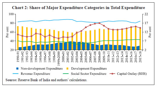 Finally, in view of the targets set by states under fiscal rules in terms of fiscal deficit, the cyclicality of GFD-GSDP ratio is also examined in the paper. Under the fiscal rules, the limits on GFD-GSDP ratio are likely to produce a pro-cyclical fiscal policy as the reduction in tax collection during slowdown would necessitate government to curtail expenditure to adhere to the targets. However, if the government borrows and prevents expenditure cutback despite lower taxes during slowdown, it would lead to a counter-cyclical policy. This would be reflected in an increase in GFD-GSDP ratio during the slowdown. Also, if fiscal space is available with a state (for example, if the GFD-GSDP ratio is less than the target), then it can go for higher expenditure and higher deficit even in the case of shortfall in revenue. It is, therefore, useful to examine the cyclicality of fiscal policy based on GFD-GSDP ratio. Correlation-based Approach This approach uses the cyclical components of fiscal variables and real GSDP. The cyclical components of real GSDP, real development expenditure, real capital outlay and GFD-GSDP ratio were obtained using the Hodrick-Prescott filter. Correlation coefficients of cyclical real GSDP with cyclical components of fiscal variables for each state for both the pre-FRL and post-FRL periods are given in Table 2. | Table 2: Correlation Coefficients of Cyclical Real GSDP with Cyclical Components of Fiscal Variables | | State | Development Expenditure | Capital Outlay | GFD-GSDP Ratio | | Pre-FRL | Post-FRL | Pre-FRL | Post-FRL | Pre-FRL | Post-FRL | | Andhra Pradesh | 0.69***
(0.00) | 0.16
(0.58) | 0.19
(0.50) | 0.35
(0.24) | 0.30
(0.27) | -0.02
(0.95) | | Arunachal Pradesh | 0.33
(0.23) | 0.43
(0.17) | 0.24
(0.38) | 0.13
(0.68) | 0.17
(0.53) | -0.15
(0.65) | | Assam | -0.01
(0.98) | -0.32
(0.28) | -0.26
(0.37) | -0.31
(0.30) | 0.02
(0.95) | -0.21
(0.48) | | Bihar | 0.01
(0.95) | -0.26
(0.41) | 0.06
(0.82) | -0.57**
(0.05) | -0.26
(0.32) | -0.35
(0.26) | | Chhattisgarh | 0.59
(0.29) | -0.34
(0.24) | -0.35
(0.57) | -0.09
(0.75) | 0.82*
(0.09) | -0.09
(0.76) | | Goa | 0.43*
(0.09) | 0.61**
(0.03) | 0.11
(0.66) | 0.54*
(0.07) | 0.24
(0.38) | -0.49*
(0.10) | | Gujarat | -0.21
(0.45) | 0.22
(0.47) | 0.25
(0.37) | -0.21
(0.49) | -0.07
(0.82) | 0.08
(0.80) | | Haryana | 0.27
(0.32) | 0.46
(0.11) | 0.23
(0.40) | 0.39
(0.19) | -0.04
(0.89) | 0.27
(0.38) | | Himachal Pradesh | 0.26
(0.34) | 0.36
(0.23) | 0.07
(0.80) | 0.25
(0.41) | -0.02
(0.94) | -0.30
(0.33) | | Jammu and Kashmir | 0.57**
(0.02) | 0.63**
(0.03) | -0.27
(0.32) | 0.33
(0.30) | 0.68***
(0.00) | 0.03
(0.92) | | Jharkhand | -0.26
(0.63) | -0.44
(0.17) | 0.15
(0.77) | -0.33
(0.31) | -0.08
(0.88) | -0.06
(0.85) | | Karnataka | 0.39
(0.21) | 0.42*
(0.10) | 0.39
(0.21) | 0.32
(0.22) | 0.27
(0.39) | 0.05
(0.85) | | Kerala | 0.31
(0.29) | 0.27
(0.33) | 0.13
(0.67) | 0.45*
(0.09) | 0.40
(0.17) | -0.06
(0.82) | | Madhya Pradesh | 0.50*
(0.06) | 0.27
(0.37) | -0.17
(0.55) | 0.65**
(0.02) | 0.36
(0.19) | 0.55**
(0.05) | | Maharashtra | -0.10
(0.71) | -0.52*
(0.07) | 0.03
(0.91) | -0.34
(0.25) | 0.02
(0.95) | -0.39
(0.18) | | Manipur | 0.78***
(0.00) | -0.06
(0.85) | 0.73***
(0.00) | -0.20
(0.50) | 0.66***
(0.01) | 0.38
(0.20) | | Meghalaya | 0.46*
(0.08) | 0.27
(0.40) | 0.13
(0.63) | 0.11
(0.74) | 0.02
(0.94) | 0.08
(0.83) | | Mizoram | 0.47*
(0.07) | 0.32
(0.31) | 0.13
(0.61) | 0.17
(0.58) | 0.35
(0.18) | 0.16
(0.62) | | Nagaland | 0.43
(0.11) | 0.23
(0.44) | 0.49*
(0.07) | 0.24
(0.44) | -0.07
(0.82) | -0.40
(0.17) | | Odisha | 0.02
(0.95) | 0.06
(0.84) | -0.40
(0.14) | -0.00
(0.99) | 0.04
(0.88) | 0.10
(0.73) | | Punjab | 0.14
(0.65) | -0.03
(0.92) | 0.12
(0.69) | 0.00
(0.99) | -0.17
(0.59) | 0.04
(0.88) | | Rajasthan | 0.63***
(0.01) | 0.05
(0.86) | 0.34
(0.22) | -0.17
(0.59) | -0.10
(0.74) | -0.17
(0.58) | | Sikkim | 0.27
(0.24) | -0.14
(0.73) | -0.01
(0.97) | -0.43
(0.29) | -0.10
(0.67) | 0.13
(0.75) | | Tamil Nadu | -0.05
(0.86) | -0.43
(0.11) | 0.29
(0.33) | 0.04
(0.89) | -0.30
(0.31) | -0.46*
(0.09) | | Tripura | 0.28
(0.31) | 0.61**
(0.03) | 0.39
(0.15) | 0.24
(0.43) | 0.34
(0.20) | 0.15
(0.63) | | Uttar Pradesh | 0.08
(0.79) | 0.46*
(0.09) | 0.08
(0.80) | 0.35
(0.22) | 0.01
(0.96) | 0.36
(0.21) | | Uttarakhand | -0.27
(0.66) | -0.41
(0.16) | -0.43
(0.46) | -0.41
(0.17) | -0.90**
(0.04) | -0.01
(0.96) | | West Bengal | -0.10
(0.65) | -0.11
(0.79) | -0.07
(0.78) | -0.03
(0.94) | 0.43**
(0.05) | -0.36
(0.39) | ***,**,*: Indicate statistical significance at 1 per cent, 5 per cent and 10 per cent levels, respectively.
Note: Figures in parentheses are p-values.
Source: Authors’ estimation/calculations based on data from RBI and NSO. | In the pre-FRL period, the correlation coefficients of the cyclical component of GSDP and cyclical development expenditure were positive and statistically significant for eight states, indicating pro-cyclical development expenditure (Table 3). For the remaining 20 states, the positive/negative correlation coefficients were statistically not significant implying the acyclical nature of development expenditure. In the post-FRL period, the number of states with positive and statistically significant correlation coefficients decreased to five and there was one state (Maharashtra) with negative and statistically significant correlation coefficient. With regard to capital outlay, in the pre-FRL period, the correlation coefficients were positive and statistically significant for two states indicating pro-cyclical nature of capital outlay. For the other 26 states, correlation coefficients (negative/positive) were statistically insignificant. In the post-FRL period, capital outlay was pro-cyclical in three states, counter-cyclical in one state (Bihar), and acyclical in the remaining 24 states. These results were broadly in line with the findings of an earlier study (RBI, 2014) which observed a mix of positive and negative correlation between cyclical GSDP and cyclical expenditures (total expenditure, primary revenue expenditure and capital outlay) across states. With respect to the GFD-GSDP ratio, the number of states showing pro-cyclical GFD declined from four in the pre-FRL period to one in the post-FRL period, while the number of states indicating counter-cyclical GFD increased to two in the post-FRL period from one in the pre-FRL period. | Table 3: Cyclicality of Fiscal Policy in Pre- and Post-FRL Period | | (Number of states) | | Period | Pro-cyclical | Counter-cyclical | | Development Expenditure | | Pre-FRL period | 8 | 0 | | Post-FRL period | 5 | 1 | | Capital Outlay | | Pre-FRL period | 2 | 0 | | Post-FRL period | 3 | 1 | | GFD-GDSP ratio | | Pre-FRL period | 4 | 1 | | Post-FRL period | 1 | 2 | | Source: Authors’ calculations. | Overall, the correlation analysis suggests that the development expenditure and GFD-GSDP ratio were less pro-cyclical during the post-FRL period compared with the pre-FRL period. However, literature suggests that the cyclicality analysis based on correlation approach may not give correct assessment as the magnitude of volatility in variables could be different and, therefore, the regression approach is a preferred approach to examine the cyclicality (Forbes and Rigobon, 1998; Lane, 2003; Misra and Ranjan, 2019; RBI, 2014). Regression Approach: System GMM Estimator The regression-based approach allows to control for variables other than GSDP, viz., gross transfers and fiscal space. The first lag of the GFD-GSDP ratio is expected to have an inverse relationship with development expenditure and capital outlay. The GFD in the previous year could serve as a proxy of the fiscal space available to a state. An increase in GFD would lead to an increase in expenditure on interest payments in the following year, which in turn could crowd out development expenditure and capital outlay. Chart 3 shows negative association of development expenditure-GDP ratio and capital outlay-GDP ratio with GFD-GDP ratio of the previous year. The correlation coefficients of the first lag of the GFD-GDP ratio with capital outlay-GDP ratio and development expenditure-GDP ratio for the period 1990-2018 were negative (-0.433 and -0.21, respectively). 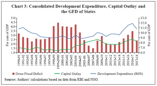 Before proceeding with system GMM estimation, the panel unit root tests were undertaken to check stationarity of the variables (Table 4). The results of all the tests employed, viz., LLC, IPS, ADF and PP indicated stationarity of the GFD-GSDP ratio and the first differences of natural logarithm of GSDP, development expenditure, capital outlay and gross transfers.4 The results of the system GMM estimator are provided in Tables 5 to 7. Table 4: Results of Panel Unit Root Tests
(sample period: 1990-2018) | | Variable | LLC t-statistics | IPS W-statistics | Fisher-ADF Chi square | Fisher-PP Chi square | | GFD-GSDP ratio | -6.18
(0.00) | -7.87
(0.00) | 165.49
(0.00) | 168.47
(0.00) | | D(log RGSDP) | -258.16
(0.00) | -91.65
(0.00) | 492.35
(0.00) | 527.92
(0.00) | | D(log devexp) | -24.14
(0.00) | -25.64
(0.00) | 546.39
(0.00) | 863.66
(0.00) | | D(log CO) | -20.74
(0.00) | -22.10
(0.00) | 475.14
(0.00) | 555.36
(0.00) | | D(log RGT) | -25.08
(0.00) | -26.10
(0.00) | 560.97
(0.00) | 853.95
(0.00) | LLC: Levin-Lin-Chu; IPS: Im-Pesaran-Shin; ADF: Augmented Dickey-Fuller;
PP: Phillips-Perron.
Note: 1. For the LLC test, the null hypothesis is ‘panels contain unit roots’; for the IPS, ADF and PP test, it is ‘all panels contain unit roots’.
2. Figures in parentheses are p-values for the relevant null hypothesis.
3. Automatic lag length selection based on SIC. | Development Expenditure The results of panel system GMM model estimated for assessing development expenditure cyclicality are given in Table 5. The log difference of real development expenditure (devexp) was regressed on log difference of real GSDP (RGSDP), first lag of GFD-GSDP ratio and log difference of real gross transfers (RGT). In view of the persistence in development expenditure growth in the post-FRL period (Chart 4), the second lag of the dependent variable was added as a regressor which was found to be statistically significant. The results suggest that development expenditure of states was pro-cyclical in both pre-FRL and post-FRL periods, as the coefficient of output variable (RGSDP) was positive and statistically significant. These results were similar to the findings of RBI (2014) and Kaur et al. (2013) in respect of education expenditure but differ from the finding in respect of social sector expenditure which was found to be acyclical by Kaur et al. (2013). However, these results were not strictly comparable with earlier studies due to differences in categories of expenditure, number of states and time period covered. Table 5: Empirical Results – Cyclicality of Development Expenditure
(Dependent Variable: Log difference of real development expenditure) | | Variable | Pre-FRL period | Post-FRL period | | 1 | 2 | 3 | | d(log devexp i, t-1) | -0.171***
(-6.40) | -0.293***
(-5.24) | | d(log devexp i, t-2) | | -0.120***
(-2.54) | | d(log RGSDPi, t) | 0.428***
(10.96) | 0.364***
(7.12) | | GFD-GSDPi, t-1 | -0.016***
(-7.08) | -0.021***
(-8.83) | | d(log RGTi, t) | 0.140***
(6.49) | 0.278***
(4.41) | | Constant | 0.097***
(7.70) | 0.121***
(16.79) | | No. of states included | 28 | 28 | | No. of Observations | 341 | 356 | Sargan test statistics
Prob>Chi2 | 22.86
(1.00) | 23.68
(1.00) | | AR (1) Test (P-value) | 0.00 | 0.00 | | AR (2) Test (P-value) | 0.32 | 0.41 | ***: Indicates statistical significance at 1 per cent level.
Note: 1. Figures in parentheses are z-statistics.
2. AR (1) and AR (2) are Arellano–Bond tests (Arellano and Bond, 1991) for first order and second order serial correlation, respectively. | The results indicate that a 1 percentage point increase in output was associated with a 0.43 percentage point increase in development expenditure in the pre-FRL period and 0.36 percentage point in the post-FRL period suggesting that development expenditure was less pro-cyclical during the post-FRL period. The results of the system GMM model corroborate the findings of the correlation analysis where fewer states showed a pro-cyclical development expenditure in the post-FRL period. Fiscal space created by states through a compression of non-development revenue expenditure might have provided headroom to avoid cutback in discretionary development expenditure during times of economic slowdown in the post-FRL period. 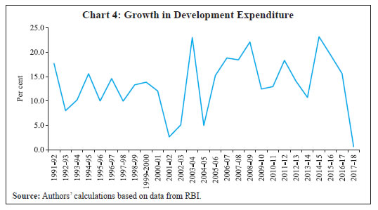 The negative and statistically significant coefficient of the lagged GFD-GSDP ratio, which is observed for both the pre- and post-FRL periods, implies that an increase in the GFD-GSDP ratio was followed by a decline in growth rate of development expenditure in the next year. Gross transfers from the Centre led to increased development expenditure of states in both the pre- and post-FRL periods. However, the impact was stronger in the post-FRL period compared to that in the pre-FRL period, which could be due to increased contribution of centrally sponsored schemes during the 2000s.5 The negative and significant coefficient of lagged dependent variable suggests discretionary nature of development expenditure. The results of Sargan test, which verifies the validity of the instruments for over-identifying restrictions, were found to be satisfactory. Further, AR (1) and AR (2) tests (used to check first order and second order serial correlation, respectively) satisfy an important assumption for the consistency of system GMM estimator. Capital Outlay Capital outlay, which forms a small proportion of the total expenditure of states (average 12.2 per cent during 1990-2018), showed a volatile pattern of growth (Chart 5). Further, the growth of capital outlay also exhibited persistence. Therefore, the second lag of dependent variable was added as a regressor which was found to be statistically significant (Table 6). The coefficient of GSDP was statistically insignificant in both pre- and post-FRL periods suggesting acyclical nature of capital outlay in both the periods. The results differ from RBI (2014) that showed pro-cyclical behaviour of capital outlay which could be due to different sample size (both in terms of number of states and time period). Among other variables, the first lag of GFD-GSDP ratio was found to be negatively associated with capital outlay. Further, as expected, the GFD-GSDP ratio seems to have stronger impact on the capital outlay than on the development expenditure. Similar to development expenditure, the coefficient of gross transfers was found to be higher in the post-FRL period compared with that in the pre-FRL period. However, the coefficient of gross transfers in the case of capital outlay was higher than that for development expenditure in both pre- and post-FRL periods. 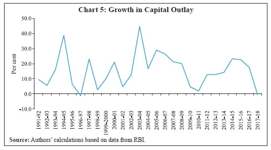
Table 6: Empirical Results – Cyclicality of Capital Outlay
(Dependent Variable: Log difference of real capital outlay) | | Variable | Pre-FRL period | Post-FRL period | | 1 | 2 | 3 | | d(log CO i, t-1) | -0.348***
(-15.40) | -0.325***
(-3.17) | | d(log CO i, t-2) | -0.315***
(-24.67) | -0.255***
(-3.10) | | d(log RGSDPi, t) | 0.106
(0.34) | -0.217
(-0.44) | | GFD-GSDPi, t-1 | -0.035***
(-7.46) | -0.029***
(-5.84) | | d(log RGTi, t) | 0.307***
(8.35) | 0.354***
(3.71) | | Constant | 0.200***
(7.49) | 0.205***
(5.73) | | No. of states included | 28 | 28 | | No. of Observations | 341 | 356 | Sargan test statistics
Prob>Chi2 | 21.25
(1.00) | 20.67
(1.00) | | AR (1) Test (P-value) | 0.05 | 0.01 | | AR (2) Test (P-value) | 0.59 | 0.28 | ***: Indicates statistical significance at 1 per cent level.
Note: 1. Figures in parentheses are z-statistics.
2. AR (1) and AR (2) are Arellano–Bond tests (Arellano and Bond, 1991) for first order and second order serial correlation, respectively. | Gross Fiscal Deficit Table 7 reports the estimation results for GFD cyclicality. Following Gavin and Perotti (1997)6, the GFD-GSDP ratio was regressed on log difference of RGSDP and the log difference of RGT. The coefficient of RGSDP was positive and statistically significant in the pre-FRL period.7 In the post-FRL period, the coefficient of RGSDP was positive but statistically insignificant. This suggests that the GFD was pro-cyclical in the pre-FRL period and acyclical in the post-FRL period. The negative and statistically significant coefficient of RGT in pre- and post-FRL periods was along expected lines as most of the gross transfers are in the form of revenue account transfers, i.e., share in central taxes and grants (accounting for 85 per cent of gross transfers during 1990-2018), which help in reducing GFD. The coefficient of lagged dependent variable was positive and significant in both the periods, but the smaller size of the coefficient in the post-FRL period indicates that the introduction of fiscal rules helped in lowering the persistence of fiscal deficit. Table 7: Empirical Results – Cyclicality of Gross Fiscal Deficit
(Dependent Variable: GFD-GSDP ratio) | | Variable | Pre-FRL period | Post-FRL period | | 1 | 2 | 3 | | GFD-GSDPi, t-1 | 0.305***
(35.69) | 0.217***
(7.72) | | d(log RGSDPi, t) | 2.73***
(2.85) | 0.090
(0.14) | | d(log RGTi, t) | -3.51***
(-13.76) | -3.01***
(-10.21) | | Constant | 3.12***
(21.20) | 2.49***
(31.94) | | No. of states included | 28 | 28 | | No. of Observations | 369 | 356 | Sargan test statistics
Prob>Chi2 | 22.87
(1.00) | 25.66
(1.00) | | AR (1) Test (P-value) | 0.00 | 0.05 | | AR (2) Test (P-value) | 0.58 | 0.29 | ***: Indicates statistical significance at 1 per cent level.
Note: 1. Figures in parentheses are z-statistics.
2. AR (1) and AR (2) are Arellano–Bond tests (Arellano and Bond 1991) for first order and second order serial correlation, respectively. | Section VI
Conclusion The fiscal position of states in India witnessed a significant improvement after the enactment of FRLs by them. The paper found that the implementation of fiscal rules by the states has had an impact on cyclicality of their fiscal policies. The assessment of cyclicality in terms of different fiscal policy variables suggested that the development expenditure turned less pro-cyclical in the post-FRL period. Capital outlay, however, showed acyclical behaviour in both pre- and post-FRL periods. The GFD of states turned acyclical in the post-FRL period from being pro-cyclical in the pre-FRL period. The findings of the paper, therefore, indicates that the adoption of fiscal rules reduces the pro-cyclicality of fiscal policy. The fiscal rules regime also assisted in enforcing fiscal discipline at the state level in India. Therefore, it may be concluded that the pursuance of a rule-based fiscal policy can play an effective role in macroeconomic management by allowing to follow counter-cyclical/less pro-cyclical fiscal policy.
References Aghion, P. & Marinescu, I. (2008). Cyclical budgetary policy and economic growth: What do we learn from OECD panel data? NBER Macroeconomics Annual 2007, 22, 251–78. Aizenman, J., Jinjarakb Y., Nguyenb, H. T. K., & Partkc, D. (2019). Fiscal space and government-spending and tax-rate cyclicality patterns: A cross-country comparison, 1960–2016, Journal of Macroeconomics, 60(C), 229–52. Alesina, A., & Bayoumi, T. (1996). The costs and benefits of fiscal rules: Evidence from U.S. States, NBER Working Paper Series, No. 5614. Arellano, M., & Bover, O. (1995). Another look at the instrumental variable estimation of error-components models, Journal of Econometrics, 68(1), 29–51. Arellano, M., & Bond, S. (1991). Some tests of specification for panel data: Monte Carlo evidence and an application to employment equations, The Review of Economic Studies, 58, 277–97. Blundell, R., & Bond, S. (1998). Initial conditions and moment restrictions in dynamic panel data models, Journal of Econometrics, 87, 115–43. Bova, E., Carcenac, N., & Guerguil, M. (2014). Fiscal rules and the procyclicality of fiscal policy in the developing world, IMF Working Paper, WP/14/122. Buiter, W. H., & Patel, U. R. (2010). Fiscal rules in India: Are they effective? NBER Working Paper Series, No. 15934. Chakraborty, P., & Dash, B. B. (2017). Fiscal reforms, fiscal rule, and development spending: How Indian states have performed?’ Public Budgeting and Finance, 37(4), 111–33. Choi, I. (2001). Unit root test for panel data, Journal of International Money and Finance, 20(2), 249-72. Cicek, D., & Elgin, C. (2011). Cyclicality of fiscal policy and the shadow economy, Empirical Economics, 41(3), 725–37. Clemens, J., & Miran, S. (2012). Fiscal policy multipliers on subnational government spending, American Economic Journal: Economic Policy, 4(2), 46–68. Fatas, A., & Mihov, I. (2006). The macroeconomic effects of fiscal rules in the US states, Journal of Public Economics, 90(1–2), 101–117. Forbes, K., & Rigobon, R. (1998). No contagion, only interdependence: Measuring stock market co-movements, NBER Working Paper Series, No. 7267. Finance Commission (2004). Report of the Twelfth Finance Commission (2005-10), Government of India, https://fincomindia.nic.in/writereaddata/html_en_files/oldcommission_html/fcreport/Report_of_12th_Finance_Commission/12fcreng.pdf Gavin, M., & Perotti, R. (1997). Fiscal policy in Latin America, NBER Macroeconomics Annual 1997, 12, 11–72. Government of India (GoI) (2017). ‘Chapter VI: Fiscal rules: Lessons from the states’, Economic Survey 2016–17, I, 113–27. Goyal, A., & Sharma, B. (2015). Government expenditure in India: Composition, cyclicality and multipliers, IGIDR Working Paper, WP-2015-032. Grembi, V., Nannicini, T., & Troiano, U. (2016). ‘Do fiscal rules matter?’, American Economic Journal: Applied Economics, 8(3), 1–30. Guerguil, M., Mandon, P., & Tapsoba, R. (2016). Flexible fiscal rules and countercyclical fiscal policy’ IMF Working Paper, WP/16/8. Ilzetzki, E., & Vegh, C. A. (2008). Procyclical fiscal policy in developing countries: Truth or fiction? NBER Working Paper Series, No. 14191. International Monetary Fund (IMF) (2017). Fiscal rules dataset 1985–2015. https://www.imf.org/external/datamapper/fiscalrules/map/map.htm Im, K. S., Pesaran, H., & Shin, Y. (2003). Testing for unit roots in heterogeneous panels, Journal of Econometrics, 115(1), 53–74. Jain, R., & Kumar, P. (2013). Size of government expenditure multipliers in India: A structural VAR analysis, RBI Working Paper, No. 7. Kaur, B., Misra, S., & Suresh, A. K. (2013). Cyclicality of social sector expenditures: Evidence from Indian states. Reserve Bank of India Occasional Papers, 34(1 & 2), 1–36. Lane, P. R. (2003). The cyclical behaviour of fiscal policy: Evidence from the OECD, Journal of Public Economics, 87(12), 2661–75. Levin, A., Lin, C., & Chu, C. J. (2002). Unit root tests in panel data: Asymptotic and finite sample properties, Journal of Econometrics, 108(1), 1–24. Maddala, G.S., & Wu, S. (1999). A comparative study of unit root tests with panel data and a new simple test, Oxford Bulletin of Economics and Statistics, 61, 631-52. Manasse, P. (2005). Deficit limits, budget rules, and fiscal policy, IMF Working Paper, WP/05/120. Marneffe, W., Bas, V. A., Wielen, W. V. D., & Vereeck, L. (2010). The impact of fiscal rules on public finances: Theory and empirical evidence for the Euro area, CESifo Working Paper, No. 3303. Mcgranahan, L., & Mattoon, R. (2012). Revenue cyclicality and changes in income and policy, Public Budgeting & Finance, 32(4), 95–119. Misra, S., & Ranjan, R. (2019). Fiscal rules and procyclicality: An empirical analysis, Indian Economic Review, 53(1–2), 207–228. Nerlich, C., & Reuter, W. H. (2015). Fiscal rules, fiscal space and procyclical fiscal policy, ECB Working Paper, No. 1872. Reserve Bank of India (RBI) (1997). Report of the Committee on Capital Account Convertibility. https://rbidocs.rbi.org.in/rdocs/PressRelease/PDFs/2450.pdf —. (2014). ‘Chapter VI: Cyclicality in the fiscal expenditures of major states in India’, State Finances: A Study of Budgets of 2013–14. Simone, A. S., & Topalova, P. (2009). India’s experience with fiscal rules: An evaluation and the way forward, IMF Working Paper, WP/09/175. Tapsoba, R. 2012. Do national numerical fiscal rules really shape fiscal behaviours in developing countries? A treatment effect evaluation, ’Economic Modelling, 29(4), 1356–69. Vegh, C. A., & Vuletin, G. (2011). How is tax policy conducted over the business cycle? NBER Working Paper Series, No. 17753. —. (2012). Overcoming the fear of free falling: Monetary policy graduation in emerging markets, NBER Working Paper Series, No. 18175.
Appendix Fiscal Responsibility Legislations at State Level: Major Features | State | Month and year of enactment of FRL | GFD-GDSP ratio of 3 per cent | Revenue deficit
elimination/revenue surplus | Target for liabilities | Expenditure target | Ceiling on guarantees | | Andhra Pradesh | June 2005 | √ | √ | 35 per cent of GSDP | – | Risk weighted guarantees at 90 per cent of RR. | | Arunachal Pradesh | March 2006 | √ | √ | – | Expenditure policies to provide impetus to economic growth, poverty reduction and improvement in human welfare. Expenditure management consistent with revenue generation. Protecting ‘high priority development expenditure’. | – | | Assam | September 2005 | √ | √ | 45 per cent of GSDP including guarantees | Ceiling on revenue expenditure under annual state plan. | 50 per cent of own revenues or 5 per cent of GSDP. | | Bihar | April 2006 | √ | √ | – | Expenditure policies to provide impetus to economic growth, poverty reduction and improvement in human welfare. Norms for prioritisation of capital expenditure. | – | | Chhattisgarh | September 2005 | √ | √ | – | – | – | | Goa | May 2006 | √ | √ | 30 per cent of GSDP | – | Ceiling as per Goa Guarantees Act. | | Gujarat | March 2005 | √ | √ | 30 per cent of GSDP | – | Cap as per Gujarat Guarantees Act. | | Haryana | July 2005 | √ | √ | 28 per cent of GSDP | – | – | | Himachal Pradesh | April 2005 | | √ | – | – | 80 per cent of RR. | | Jammu and Kashmir | August 2006 | √ | √ | 55 per cent of GSDP | Expenditure policies to provide impetus to economic growth, poverty reduction and improvement in human welfare. Norms for prioritisation of capital expenditure. | Risk weighted guarantees at 75 per cent of RR. | | Jharkhand | May 2007 | √ | √ | 300 per cent of RR by 2007-08 | Expenditure policies to provide impetus to economic growth, poverty reduction and improvement in human welfare. Expenditure management consistent with revenue generation. | – | | Karnataka | September 2002 | √ | √ | – | – | – | | Kerala | August 2003 | 3.5 per cent by 2005-06 and 2.0 per cent by 2006-07 | √ | – | – | – | | Madhya Pradesh | May 2005 | √ | √ | 40 per cent of GSDP | – | 80 per cent of RR. | | Maharashtra | April 2005 | Shall specify by rule, target reduction | √ | – | – | | | Manipur | August 2005 | √ | √ | – | Salary bill not to exceed 35 per cent of RE (excluding interest payment and pension). Expenditure policies to provide impetus to economic growth, poverty reduction and improvement in human welfare. | As per Manipur Guarantees Act. | | Meghalaya | March 2006 | √ | √ | 28 per cent of GSDP | Expenditure policies to provide impetus to economic growth, poverty reduction and improvement in human welfare. Expenditure management in relation to receipts potential. Efforts to contain non-plan expenditure. Reduce expenditure on wages and salaries. | – | | Mizoram | October 2006 | √ | √ | – | Expenditure policies to provide impetus to economic growth, poverty reduction and improvement in human welfare. Norms for prioritisation of capital expenditure. | Risk weighted guarantees not to exceed twice of consolidated fund receipts. | | Nagaland | August 2005 | √ | √ | 40 per cent of GSDP | Salary bill not to exceed 61 per cent of RE (excluding interest payment and pension). Expenditure policies to provide impetus to economic growth, poverty reduction and improvement in human welfare. | Risk weighted guarantees at 1 per cent of RR/ GSDP. | | Odisha | June 2005 | √ | √ | 300 per cent of RR by 2007-08 | – | – | | Punjab | October 2003 | √ | √ | 40 per cent by 2006-07 | – | 80 per cent of RR. | | Rajasthan | May 2005 | √ | √ | Debt (excluding public account) not to exceed twice of consolidated fund receipts. | – | – | | Sikkim | September 2010 | √ | √ | – | – | – | | Tamil Nadu | May 2003 | √ | √ | – | – | 100 per cent of RR or 10 per cent of GSDP. | | Tripura | June 2005 | √ | √ | 40 per cent of GSDP | – | Risk weighted guarantees to 1 per cent of GSDP. | | Uttarakhand | October 2005 | √ | √ | 25 per cent of GSDP by March 2015 | Expenditure policies to provide impetus to economic growth, poverty reduction and improvement in human welfare. Expenditure management consistent with revenue generation. Protecting ‘high priority development expenditure’. | No guarantee beyond state stipulated limit. | | Uttar Pradesh | February 2004 | √ | √ | 25 per cent of GSDP by March 2018 | As per the target in MTFP. | No guarantee beyond state stipulated limit. | | West Bengal | July 2010 | √ | √ | – | – | – | Note: RE: Revenue Expenditure, RR: Revenue Receipts, MTFP: Medium Term Fiscal Policy Plan
Source: State Finances: A Study of Budgets (various issues), RBI. |
|