Dipak R. Chaudhari, Sarat Dhal and Sonali M. Adki^*

In this study, we postulate currency demand for transaction purposes driven by income effect, and a payment technology induced substitution effect working through velocity of currency. Innovations in payment systems have shown a statistically significant long-run inverse relationship with currency demand in India. However, the magnitude of its coefficient indicates that the substitution effect on currency demand could be smaller than the dominant income effect. In the presence of payment indicators and financial variables, the income effect coefficient on currency demand has come closer to unity, in line with the standard quantity theory of money but different from the inventory theoretic transaction demand model prediction (0.5). The impact of 1 per cent growth in digital retail transactions volume was estimated to be one tenth of the income effect. Thus, to neutralise the dominant income effect, the payment systems need rapid growth to the extent of 100 per cent in digital retail transactions volume.

JEL Classification: E41, E47, E51, C22

Keywords: Money demand, monetary policy, payment system, error correction and cointegration, ARDL model

Introduction

India’s payment systems have witnessed significant growth in digital transactions, supported by policy thrust, sustained efforts from banking and financial sectors to provide technology enabled services and consumers’ adoption of various non-cash payment instruments. At the same time, the demand for currency also exhibits growth momentum. Illustratively, currency in circulation to GDP ratio, after declining from 12.1 per cent in 2015-16 to 8.7 per cent in 2016-17 in the wake of demonetisation¹, recovered to 10.7 per cent in 2017-18 and 11.2 per cent in 2018-19. In this context, a question arises on the impact of payments technology innovation on currency demand. The empirical studies for a cross-section of countries do not offer unique answers. A common perspective is that the relationship of payment systems with currency demand can be country specific. Therefore, we examine this relationship in the Indian context. We analyse currency demand as a function of payment indicators along with other proximate determinants such as income and financial variables (interest rate on deposits and stock return). We are specifically interested in assessing whether payment indicators could impinge on long-run currency demand, for which we use the autoregressive distributed lag (ARDL) model based on quarterly data. The rest of the study is organised into seven sections. Section II provides details of the policy approach to payment systems development in India. Section III reviews the existing literature on payment systems. Section IV gives details of the analytical framework used in this study. Section V discusses data and empirical modelling. Section VI explains stylised facts, Section VII explains empirical findings, and Section VIII concludes the study.

Section II
Payment Systems Development: India’s Policy Approach

The central bank of a country is usually the driving force behind the development of national payment systems. India’s central bank, the Reserve Bank of India (RBI), has been playing this developmental role and has taken several initiatives for safe, secure, sound, efficient, accessible and authorised payment systems in the country (Gupta and Gupta, 2013). A chronology of major initiatives since the late 1980s in the Indian payment systems is given in the Appendix (Table A.1).

The initial steps towards establishing modern payment systems were taken in the early 1980s, when the RBI introduced the magnetic ink-character recognition (MICR) technology for cheque processing, which sowed the seeds for digital payment systems in the country. Migration to the cheque truncation system (CTS) happened in 2008, when the RBI first implemented it in New Delhi, on February 1, 2008 with 10 pilot banks. Soon thereafter the deadline was set to April 30, 2008 for all banks to migrate to the CTS. Further, to handle bulk payments and receipts, the electronic clearing system (ECS) was introduced, which has undergone many changes from being local to regional and then national. For a pan-India system for processing bulk and repetitive payments, the ECS has been subsumed into the National Automated Clearing House (NACH). The next step towards electronic products was the introduction of interoperable ATMs, wherein the National Financial Switch (NFS) had proved that in a large country like India, networked ATMs can function very well.

Payment systems have evolved over time to meet the requirement of remittances using non-cash and non-paper payment methods. The popularly known retail system is the National Electronic Funds Transfer (NEFT). Besides NEFT, the Immediate Payment Service (IMPS) and Real-time Gross Settlement (RTGS) also meet users’ funds transfer requirements. Recently, the NEFT has been made operational on a 24x7 basis from December 16, 2019 to ensure availability of digital payments at any time. The IMPS is also a 24x7 immediate funds transfer system. The RTGS is meant for processing large value transactions of above ₹200,000, apart from interbank transactions. The modernisation of the information technology (IT) systems of banks and their core banking solutions has made possible the integration of various delivery channels. The large number of mobile phone users and the availability of cost-effective internet data have led to an increase in the number of mobile internet users. Taking advantage of this, an increasing number of payment facilities are being integrated through the mobile channel. Further, the introduction of a unified payment interface (UPI) has revolutionised the mobile payment system.

A wide range of reforms have been introduced to promote digital payments, covering customer-initiated transactions and government payments. From the perspective of financial inclusion and digitisation of government payments, the use of Aadhaar² for beneficiary identification and authentication in payments has played an important role, enhancing efficiency and transparency in transactions. Accordingly, the Aadhaar Payment Bridge System (APBS) has been put in place to facilitate bulk and repetitive government payments to Aadhaar-seeded bank accounts of identified beneficiaries. Similarly, the Aadhaar Enabled Payment System (AePS) facilitates operations from Aadhaar-seeded bank accounts using biometric authentication of customers. Today, AePS is increasingly being used for Business Correspondent (BC) operations in an interoperable manner. Another significant segment of retail electronic payments is the RuPay cards issued under the Pradhan Mantri Jan Dhan Yojana, with its associated benefits dependent upon usage of the card.

The entry of non-bank players in payment systems has made an important contribution in terms of innovations and convenience to customers. Besides setting up White Label ATMs (WLAs) to bridge the gap in ATM infrastructure in rural and semi-urban areas in the country, non-banks are actively involved in issuance of Pre-paid Payment Instruments (PPIs). There are many payment systems with significant potential to influence the payment habits of different individuals. The Bharat Bill Payment System (BBPS) provides facility of anytime, anywhere, anyhow bill payments in the country and supports all forms of electronic payments. Also, the Trade Receivables Discounting System (TReDS) caters to the financing needs of the micro, small and medium enterprises (MSMEs) for faster financing and liquidity requirements. Thus, the retail payments ecosystem has made revolutionary progress over the years. The standards of all the payment channels and systems along with their security features in India are comparable with the best in the world. Compared with other countries, the changes in India’s payments ecosystem have been fast-forwarded to reach its present stage in the shortest possible time. User trust in the payments system is being strengthened through policy initiatives over the years with implementation of certain policies relating to cyber security, fraud, customer awareness, and customer protection. Finally, the RBI has released its payment vision documents in the public domain. According to the latest document, ‘Payment and Settlement Systems in India: Vision 2019-2021’³, digital transactions through UPI/IMPS are likely to register average annualised growth of over 100 per cent, which would help in the reduction of currency demand over the vision period.

Section III
The Literature

Economics literature on payment systems has evolved in various dimensions, broadly through macroeconomic and microeconomic perspectives (Kahn and Roberds, 2009). The macroeconomic perspective focuses on the impact of payment technology on currency and money demand (Amromin and Chakravorti, 2007; Bech et al., 2018; Columba, 2009; Duca and VanHoose, 2004; Durgun and Timur, 2015; Fischer, 2007; Humphrey, 2004 and 2010; Lippi and Secchi, 2009; Oyelami and Yinusa, 2013). Some studies address the liquidity effects of payment systems (Li and Carroll, 2011), while some others consider the substitution effect of mode of payments (Schuh and Stavins, 2010). On the other hand, microeconomic studies offer perspective on the various determinants affecting the behaviour of people towards the adoption of modern payment instruments and alternate money such as the availability of technology, internet facility and education (Basnet and Donou-Adonsou, 2016; Lippi and Secchi, 2009), card prices (Hazra, 2017; Scholnick et al., 2008), switching and search costs (Ausubel, 1991; Calem and Mester, 1995; Calem et al., 2006; Stango, 2002), interest cost impact on card debt (Brito and Hartley, 1995; Lee, 2014), transaction cost and opportunity cost (Klee, 2008), impact of rewards, discounts and incentives on the use of credit and debit cards (Arango et al., 2015; Arango-Arango et al., 2018; Simon et al., 2010; Stavins, 2018; Valverde and Zegarra, 2011), impact of safety and security aspects (Eze et al., 2008; Kosse, 2013), usefulness of record-keeping of electronic payment data (Galbraith and Tkacz, 2018; Lotz and Zhang, 2016), consumer preference for a specific payment instrument and the impact of price elasticity on instrument choice (Stavins, 2018) and the evidence of beta convergence in the European countries’ payment system (Martikainen et al., 2015).

The literature provides mixed evidence on the role of payment systems innovation on money and currency demand. The differential impact is largely due to differences in payment instruments. Illustratively, using disaggregated provincial data in Italy, Columba (2009) shows that innovations in transaction technology through diffusion of ATMs and POS have a negative effect on the demand for currency in circulation but a positive effect on narrow money demand due to the positive effect of technology on bank deposits. Bouhdaoui et al. (2014) analyse the relationship between convenient prices⁴ and cash usage by French nationals and find that individuals’ shares of cash payments increased with convenient prices. Clearly, price rigidity can, in part, be explained by the use of cash to pay convenient prices. For Japan, Fujiki and Tanaka (2014), using household-level survey data and a quantile regression model, provide evidence that users of electronic money held more currency than non-users. Bech et al. (2018), using a cross-country (advanced and emerging market economies) panel data model, suggest that despite the increasing use of digital payments across the world, cash continues to be the more preferred mode of payment due to store of value motive and lower opportunity cost rather than payment needs. Some studies also find modern payment instruments to have a positive effect on tax collection – cashless payments reduce tax evasion as the transactions can be tracked easily by the authorities (Hondroyiannis and Papaoikonomou, 2017; Immordino and Russo, 2018).

In the case of developing nations, Oyelami and Yinusa (2013), using data on the Nigerian economy, provide evidence that internet payments and mobile money substituted currency while credit cards, Automated Teller Machine (ATM) and Point of Sale (POS) complimented it. Moreover, barring ATM debit cards and internet payments, all payment channels showed an inverse relationship with shocks to the interest rate and currency demand. This finding may have serious implications for how monetary policy is implemented, especially in developing countries. For India, Nachane et al. (2013) find that despite the emergence of various alternatives to cash-based transactions, currency retained its predominance. There exists a cointegrating relationship between currency in circulation, gross domestic product (GDP), wholesale price index (WPI) and deposit rates. The RBI report on the macroeconomic impact of demonetisation (RBI, 2017) analyses growth rates in various payment channels, observing that an important consequence of demonetisation has been the sharp increase in the use of digital transactions. Maiti (2017) finds that post demonetisation cash transactions have moved in a sustained manner to non-cash modes of payment. Reddy and Kumarasamy (2017) examine the impact of credit and debit cards usage on currency demand in India by employing the ARDL approach. Their results show that the usage of credit cards is negatively associated with currency demand, whereas the usage of debit cards shows a positive association with currency demand in India.

Some studies find that payment technology innovation can also affect income effect on transaction demand for currency and money. In the case of Switzerland, Fischer (2007) re-examines the estimates for income elasticity of money demand based on cross-regional (cantonal) data. The study estimates that income elasticity can range between 0.4 and 0.6. On the contrary, Kumar (2011) analyses data on 20 developing Asian and African countries and finds that the magnitude of income elasticity did not change significantly with the increase in the use of modern payment systems. In the case of India, the income elasticity of currency demand is somewhat higher in comparison to the long-term elasticity observed in similar studies for advanced countries (Nachane et.al., 2013).

Section IV
Analytical Approach

From a theoretical perspective, the role of payment systems in currency demand derives from its impact on the velocity of money (Meltzer, 1978). Let us consider the standard quantity theory of money or Fisher’s version of the transaction demand for money M (currency with public), driven by velocity of money in circulation (V), economic activity (Y) and general price level (P):

Section V
Data and Empirical Modelling

For the econometric estimation of currency demand in line with the current literature and analytical insights, we use an autoregressive distributed lag (ARDL) model owing to Pesaran and Shin (Pesaran et al., 2001). The choice of the model is partly determined by the sample period for which the data is available. Illustratively, data on currency with the public, part of money demand are available for a very long period from 1950-1951. However, quarterly data on its main determinant, the aggregate income or GDP, are available only from 1996-1997. On the other hand, payments indicators data are available on a monthly basis from April 2004, allowing us to generate quarterly series data for the sample period 2004:2 to 2019:1. Thus, we have a common sample period 2004:2 to 2019:1, i.e., about 60 quarters data, which is not sufficiently large to allow time series models such as vector autoregression (VAR) and vector error correction (VEC) models. Moreover, the advantage of the ARDL model is that it can encompass a mix of stationary and non-stationary variables and allows the estimation of short-run error correction and long-run cointegration relationships among the variables. Since the ARDL model is quite popular, we have avoided offering its technical details.

The ARDL is preferred to other cointegration methods by Engle and Granger (1987), Johansen (1991), and Johansen and Juselius (1990) for various reasons: (i) it provides unbiased estimates of long-run model and valid t-statistics, even when some of the explanatory variables are endogenous (Ali et al., 2016); (ii) it also facilitates short-run analysis: the dynamic error correction model is derived from a simple linear transformation in the ARDL model; and (iii) being a single equation approach, it can be suitable to a smaller sample. However, the model is not applicable if the order of integration of any of the variables is greater than one, for example, I(2) variable (Menegaki, 2019). In this case, the critical bounds provided by Pesaran et al. (2001) and Narayan (2005) are not valid. The ARDL procedure involves two stages. The first stage is to establish the existence of a long-run relationship. Once such a relationship is established, a two-step procedure is used to estimate the long-run and short-run coefficients of the same equation in the error correction framework. The existence of the long-run relationship is confirmed with the help of an F-test to determine that the coefficients of all explanatory variables are jointly different from zero (Menegaki, 2019). A notable aspect of our empirical exercise is that the payment indicators data exhibit large shifts, reflecting the introduction of new instruments. Large outliers could give rise to biased estimates. In order to overcome this problem, we use the TRAMO/SEATS approach developed by Gómez and Maravall (1995) to derive smooth linearised series for the payment indicators.

Section VI
Stylised Facts

Table 1 provides summary statistics (sample mean, median, standard deviation, etc.) of growth rates of currency in circulation, real GDP growth, CPI inflation, and growth of payment indicators in volume and value terms for the period 2004:Q2-2019:Q1. The average growth in payment indicators, both in value and volume terms was two to three times larger than currency growth and four to five times larger than the GDP growth and inflation rate over the sample period.

Table 2 provides summary statistics of nominal and real interest rates and asset returns (equity and gold) which denote the opportunity cost of holding money. During the sample period, real interest rates on bank deposits and medium-term government bond yield (5-year maturity) show a mean of 0.6 percentage points, while assets like equity and gold show higher real returns.

Section VII
Empirical Findings

Since the ARDL method is not applicable when the variables are I(2), we conducted the standard augmented Dickey-Fuller test (ADF) method of unit root test for currency, income and payment system indicators. The unit root test results (Appendix Table A.2) suggest that none of the variables considered in the paper could be characterised with the I(2) process. Hence, the ARDL model could be used for empirical estimation. Since our objective is to examine the long-run impact of payment indicators on currency demand, we begin with the baseline model (M1) that does not include payment indicators and then include alternative payment indicators measured in volume terms in the other models. The different models include different payment indicators, such as retail electronic clearing (REC) including ECS and NEFT (M2), card transactions at POS (M3), retail transactions such as ECS, NEFT, card transactions at POS (M4) and all-digital transactions including BHIM and IMPS (M5). Table 3 provides a summary of the estimated results of the long-run demand function for currency measured in real terms. We derive some interesting perspectives from the estimated cointegrating equations.

First, across the models M2 to M5, coefficients associated with payment indicators have plausible negative sign. Except retail clearing, all other payment indicators have statistically significant coefficients. Thus, in general, we find that the volume growth of non-cash digital payments has a moderating effect on currency demand. Second, the impact differs across payment indicators, as evident from the magnitude of coefficients; illustratively, the coefficient of a narrow measure like POS transactions is twice the coefficient of a broader measure like an all-digital transactions. Third, a crucial finding pertains to the income effect on currency demand, when we compare models with payment indicators (M2 to M5) to models without it (M1). The coefficient of income variable (real GDP) increases when payment indicators are included in the regression, while the intercept term, which captures the deterministic component of velocity, or the scale effect, becomes much smaller. Here, our findings are consistent with the literature (Columba, 2009; Nachane et al., 2013). Fourth, the coefficient of error correction (EC) term associated with the ARDL model, which indicates the speed of adjustment to a long-run path following a short-run deviation, also indicates the role of technology. The EC coefficient is negative and statistically significant, and larger in absolute size for the currency demand equation including payment indicator, than for the equation without it. This implies that payment indicators foster currency demand’s adjustment to long-run path through its impact on velocity induced effect.

Table 4 shows the estimates of the long-run demand function for currency in nominal terms. The explanatory variables are nominal GDP and alternative payment indicators measured in volume terms. The results are comparable with the equation estimated for real currency demand, and they provide some notable insights. First, we obtain a statistically significant inverse relationship of payment indicators with currency demand as was the case in the equation for currency demand in real terms. Second, the income elasticity of demand for money without payment indicators is closer to unity but remains above unity when payment indicators are included. Compared with the real currency demand function, nominal income elasticity shows some moderation. Third, the absolute size of the coefficient of payment indicators shows some moderation. Fourth, the size of the intercept term in absolute terms is substantially lower in a nominal demand function.

Next, we examine the impact of payment indicators taken in value terms on currency demand. We estimate both nominal and real currency demand functions. The estimates of nominal currency demand equation are given in Table 5. The retail electronic clearing and POS indicators show a statistically significant inverse relationship with currency demand. On the contrary, the coefficient of broader measures of payments indicator (all-digital) is negative but statistically not significant.

Results for the real currency demand seem implausible barring the card transactions indicator (Table 6). In the regression equations incorporating all other payment indicators, the coefficient of income is statistically not significant, which seems counter-intuitive. Thus, it is evident that the impact of payments technological innovation on currency demand could be better explained when payment indicators are taken in volume terms rather than in value terms.

Next, to assess the impact of financial variables on currency demand, we estimate the equation by incorporating deposit interest rate and asset (stock) return. The equation for nominal currency demand function did not provide plausible results. The results for the equation of real currency demand function are given in Table 7. Real deposit interest rate and stock return show negative impact on currency demand, though the interest rate is statistically not significant. Overall, we can say that interest rate and asset returns can marginally influence currency demand. However, the crucial finding here is that with the presence of real interest rate and asset returns, and volume-based payment indicators, barring POS, income effect come closer to unity. Moreover, payment indicators have a statistically significant inverse relationship with currency demand. But the impact is somewhat lower than that found in the equation without financial variable (Table 3), highlighting the role of financial innovation (interest rate and stock return).

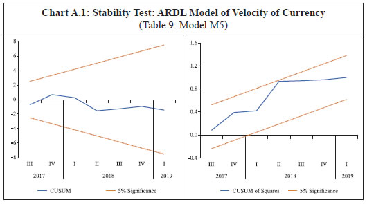
For robustness of empirical findings, it is important to reflect on the role of policy to withdraw high denomination specified bank notes (SBNs). Here, we re-estimate two of the equations M1 and M5 from Table 7 for the truncated period up to 2016:Q2; we exclude the period after November 2016 when SBNs were withdrawn from circulation (Table 8). It is crucial to note that we are omitting a small period of 11 quarters, 2016:Q3 to 2019:Q1, which may not be fully adequate to reflect on the policy regime. Nevertheless, this could provide some early reflection. Compared with counterpart equations for the full sample period in Table 7, we find that the income effect is comparable but there is a marginal improvement in the substitution effect of payment indicators on the currency demand. However, the difference in the long-run intercept term, which could reflect upon the scale effect, is somewhat noticeable. Thus, the impact of demonetisation could have impinged in moderating the scale effect on currency demand.

Furthermore, for the stability analysis, we consider the model (M5) of Table 7 and carry out CUSUM and CUSUM square test. The model passed the stability test based on CUSUM test but failed the CUSUM square test, which could be attributed to the period 2016:Q4 for which the model had a relatively larger residual. However, the model could pass the Breusch–Godfrey serial correlation LM test as shown in the estimation tables. In this context, we conclude that since the income effect could be closer to unity, the impact of technology on currency demand could be explored through its impact on velocity of currency in line with equation 5 in Section 4. The suitable ARDL model for velocity of currency, satisfying the stability consideration and no residual serial correlation, could be the one with a structural dummy variable for the period since the 2016:Q4 (Table 9 and Appendix Chart A.1). The long-run impact of broader measure of technology on velocity turned out to be statistically significant, though the coefficient size was somewhat lower than the model M5 in Table 7.

Summing up, we found payment technology innovations, as measured in terms of digital volume transactions, having a statistically significant inverse relation with India’s currency demand in the long run. However, the substitution effect of digital transactions on currency demand was lower than the strong positive income effect, which suggests that the digital transactions need to increase rapidly if the income effect on currency demand were to be neutralised.

Section VIII
Conclusion

The findings of the paper suggest that real income is the major driver of currency demand in India. The income effect of currency demand is closer to unity even when payment indicators, interest rate and asset returns are included as explanatory variables. Payment systems innovation, especially digital transactions in volume terms, showed statistically significant negative effect on currency demand. However, the coefficient of payment indicators was only about one tenth of the income coefficient. Thus, in order to neutralise the real income and inflation induced positive effect on currency demand, digital payments need to increase at a faster pace. Nevertheless, payment systems indicators with growth of around 35 per cent in volume terms during the sample period could have sizeable potential impact of around 3 per cent reduction in currency demand. Digital payments need to grow at a pace of about 100 per cent per annum in order to neutralise the income effect on currency demand. The empirical findings of the study could serve useful for policy purposes. As the payment system grows, and the sample period accumulates with more quarterly data, future studies could exploit the advanced econometric methodology and reassess the impact of technology innovations on currency demand.

References

Ali, H. S., Law, S. H., & Zannah, T. I. (2016). Dynamic impact of urbanization, economic growth, energy consumption, and trade openness on CO2 emissions in Nigeria. Environmental Science and Pollution Research, 23, 12435–43.

Amromin, G., & Chakravorti, S. (2007). Debit card and cash usage: A cross-country analysis. Federal Reserve Bank of Chicago Working Paper No. 2007-04. https://ssrn.com/abstract=981236 or http://dx.doi.org/10.2139/ssrn.981236

Arango, C., Huynh, K. P., & Sabetti, L. (2015). Consumer payment choice: Merchant card acceptance versus pricing incentives. Journal of Banking & Finance, 55, 130–141.

Arango-Arango, C. A., Bouhdaoui, Y., Bounie, D., Eschelbach, M., & Hernandez, L. (2018). Cash remains top-of-wallet! International evidence from payment diaries. Economic Modelling, 69, 38–48.

Ausubel, L. M. (1991). The failure of competition in the credit card market. The American Economic Review, 81(1), 50–81.

Basnet, H. C., & Donou-Adonsou, F. (2016). Internet, consumer spending, and credit card balance: Evidence from US consumers. Review of Financial Economics, 30, 11–22.

Baumol, W. J. (1952). The transactions demand for cash: An inventory theoretic approach. Quarterly Journal of Economics, 66, 545–556.

Bech, M. L., Faruqui, U., Ougaard, F., & Picillo, C. (2018). Payments are a-changin’ but cash still rules. BIS Quarterly Review, March.

Bouhdaoui, Y., Bounie, D., & François, A. (2014). Convenient prices, cash payments and price rigidity. Economic Modelling, 41, 329–337.

Brito, D. L., & Hartley, P. R. (1995). Consumer rationality and credit cards. Journal of Political Economy, 103(2), 400–433.

Calem, P. S., & Mester, L. J. (1995). Consumer behavior and the stickiness of credit-card interest rates. The American Economic Review, 85(5), 1327–1336.

Calem, P. S., Gordy, M. B., & Mester, L. J. (2006). Switching costs and adverse selection in the market for credit cards: New evidence. Journal of Banking & Finance, 30(6), 1653–1685.

Carbó-Valverde, S., & Liñares-Zegarra, J. M. (2011). How effective are rewards programs in promoting payment card usage? Empirical evidence. Journal of Banking & Finance, 35(12), 3275–3291.

Columba, F. (2009). Narrow money and transaction technology: New disaggregated evidence. Journal of Economics and Business, 61(4), 312–325.

Duca, J. V., & VanHoose, D. D. (2004). Recent developments in understanding the demand for money. Journal of Economics and Business, 56(4), 247–272.

Durgun, Ö., & Timur, M. C. (2015). The effects of electronic payments on monetary policies and central banks. Procedia-Social and Behavioral Sciences, 195, 680–685.

Engle, R. F., & Granger, C. W. (1987). Co-integration and error correction: Representation, estimation, and testing. Econometrica: Journal of the Econometric Society, 55(2), 251–276.

Eze, U. C., Gan, G. G. G., Ademu, J., & Tella, S. A. (2008). Modelling user trust and mobile payment adoption: A conceptual Framework. Communications of the IBIMA, 3(29), 224–231.

Fischer, A. M. (2007). Measuring income elasticity for Swiss money demand: What do the cantons say about financial innovation?. European Economic Review, 51(7), 1641–1660.

Fujiki, H., & Tanaka, M. (2014). Currency demand, new technology, and the adoption of electronic money: Micro evidence from Japan. Economics Letters, 125(1), 5–8.

Galbraith, J. W., & Tkacz, G. (2018). Nowcasting with payments system data. International Journal of Forecasting, 34(2), 366–376.

Gómez, V., & Maravall Herrero, A. (1995). Programs TRAMO and SEATS: Instructions for the user (beta version: September 1996). Banco de España. Servicio de Estudios.

Gupta, A., & Gupta, M. (2013). Electronic Mode of Payment–A Study of Indian Banking System. International Journal of Enterprise Computing and Business Systems, 2(2), 3-5.

Hazra, D. (2017). Monetary policy and alternative means of payment. The Quarterly Review of Economics and Finance, 65, 378–387.

Hondroyiannis, G., & Papaoikonomou, D. (2017). The effect of card payments on VAT revenue: New evidence from Greece. Economics Letters, 157, 17–20.

Humphrey, D. B. (2004). Replacement of cash by cards in US consumer payments. Journal of Economics and Business, 56(3), 211–225.

Humphrey, D. B. (2010). Retail payments: New contributions, empirical results, and unanswered questions. Journal of Banking & Finance, 34(8), 1729–1737.

Immordino, G., & Russo, F. F. (2018). Cashless payments and tax evasion. European Journal of Political Economy, 55, 36–43.

Johansen, S. (1991). Estimation and hypothesis testing of cointegration vectors in Gaussian vector autoregressive models. Econometrica: Journal of the Econometric Society, 59(6), 1551–1580.

Johansen, S., & Juselius, K. (1990). Maximum likelihood estimation and inference on cointegration – with applications to the demand for money. Oxford Bulletin of Economics and Statistics, 52(2), 169–210.

Kahn, C. M., & Roberds, W. (2009). Why pay? An introduction to payments economics. Journal of Financial Intermediation, 18(1), 1–23.

Klee, E. (2008). How people pay: Evidence from grocery store data. Journal of Monetary Economics, 55(3), 526–541.

Kosse, A. (2013). Do newspaper articles on card fraud affect debit card usage?. Journal of Banking & Finance, 37(12), 5382–5391.

Kumar, S. (2011). Financial reforms and money demand: Evidence from 20 developing countries. Economic Systems, 35(3), 323–334.

Lee, M. (2014). Constrained or unconstrained price for debit card payment?. Journal of Macroeconomics, 41, 53–65.

Li, Y., & Carroll, W. (2011). The payment mechanisms and liquidity effects. Journal of Macroeconomics, 33(4), 656–667.

Lippi, F., & Secchi, A. (2009). Technological change and the households’ demand for currency. Journal of Monetary Economics, 56(2), 222–230.

Lotz, S., & Zhang, C. (2016). Money and credit as means of payment: A new monetarist approach. Journal of Economic Theory, 164, 68–100.

Maiti, Sasanka Sekhar (2017). From cash to non-cash and cheque to digital: The unfolding revolution in India’s payment systems, Mint Street Memo No. 07. https://www.rbi.org.in/Scripts/MSM_Mintstreetmemos7.aspx

Martikainen, E., Schmiedel, H., & Takalo, T. (2015). Convergence of European retail payments. Journal of Banking & Finance, 50, 81–91.

Meltzer, Allan H. (1978). The Effects of Financial Innovation on the Instruments of Monetary Policy. Economies et Societies. Cahiers de L’Ismea, Vol. 12. Available at Carnegie Mellon University Research Showcase.

Menegaki, A. N. (2019). The ARDL method in the energy-growth nexus field; best implementation strategies. Economies, 7(4), 105.

Nachane, D. M., Chakraborty, A. B., Mitra, A. K., & Bordoloi, S. (2013). Modelling currency demand in India: An empirical study. Study No. 30, Development Research Group (DRG) Study Series, Reserve Bank of India, Mumbai. https://rbidocs.rbi.org.in/rdocs/Publications/PDFs/39DRGS180213.pdf

Oyelami, L. O., & Yinusa, D. O. (2013). Alternative payment systems implication for currency demand and monetary policy in developing economy: A case study of Nigeria. International Journal of Humanities and Social Science, 3(20), 253–260.

Pesaran, M. H., Shin, Y., & Smith, R. J. (2001). Bounds testing approaches to the analysis of level relationships. Journal of Applied Econometrics, 16(3), 289–326.

Reserve Bank of India (RBI) (2017). Macroeconomic impact of demonetisation: A preliminary assessment, March. https://m.rbi.org.in/Scripts/OccasionalPublications.aspx?head=Macroeconomic%20Impact%20of%20Demonetisation

Reddy, S., & Kumarasamy, D. (2017). Impact of credit cards and debit cards on currency demand and seigniorage. Academy of Accounting and Financial Studies Journal, 21(3), 1–15.

Scholnick, B., Massoud, N., Saunders, A., Carbo-Valverde, S., & Rodríguez-Fernández, F. (2008). The economics of credit cards, debit cards and ATMs: A survey and some new evidence. Journal of Banking & Finance, 32(8), 1468–1483.

Schuh, S., & Stavins, J. (2010). Why are (some) consumers (finally) writing fewer checks? The role of payment characteristics. Journal of Banking & Finance, 34(8), 1745–1758.

Simon, J., Smith, K., & West, T. (2010). Price incentives and consumer payment behaviour. Journal of Banking & Finance, 34(8), 1759–1772.

Stango, V. (2002). Pricing with consumer switching costs: Evidence from the credit card market. The Journal of Industrial Economics, 50(4), 475–492.

Stavins, J. (2018). Consumer preferences for payment methods: Role of discounts and surcharges. Journal of Banking & Finance, 94, 35–53.

Tobin, J. (1956). The Interest-Elasticity of the Transactions Demand for Cash. Review of Economics and Statistics, 38, 241–247.

Appendix

^* Sarat Dhal and Sonali M. Adki are Directors and Dipak R. Chaudhari is an Assistant Adviser in the Reserve Bank of India (RBI). The authors thank the anonymous referee, Dr. Jay Chander, Editor, RBI Occasional Papers and internal discussants of the paper for their valuable comments and suggestions. The usual disclaimer applies: the views expressed in this paper are those of the authors and do not represent the views of the RBI. Please direct all correspondence to: scdhal@rbi.org.in.

¹ The Government of India, on November 8, 2016, announced that ₹500 and ₹1,000 denomination bank notes issued by the RBI shall cease to be legal tender.

² Aadhaar is a 12-digit number issued by the Unique Identification Authority of India (UIDAI) to the residents of India based on their demographic and biometric information.

³ On May 15, 2019 the RBI announced a vision document titled ‘Payment and Settlement Systems in India: Vision 2019–2021’, with its core theme of ‘Empowering Exceptional (E) payment Experience’. The document aims to empower every Indian with access to a bouquet of e-payment options that are safe, secure, convenient, quick and affordable.

⁴ Convenient prices are round prices that usually match monetary denominations. Firms set convenient price to avoid cash payments when the cost of handling cash is high or risky (e.g. theft) compared to the costs of other payment instruments. The same reasoning applies to consumers who also face transaction and holding costs when they use cash or other payment instruments (Bouhdaoui et al., 2014).