Janak Raj, Indranil Bhattacharyya, Samir Ranjan Behera, Joice John and Bhimappa Arjun Talwar* The paper uses an array of time series and econometric techniques to analyse and forecast currency demand in India. While the weekly forecasting model includes institutional and idiosyncratic factors to generate forecasts of currency in circulation which are crucial for efficient day-to-day liquidity management operations of the Reserve Bank, the monthly model incorporates both macroeconomic factors and technological innovations in the payment system to delineate the impact of digital payments on currency demand. The quarterly and annual models incorporate macroeconomic factors to understand the long-run determinants and short-run dynamics of currency demand. The key findings emerging from the study are: (i) currency in circulation shows weekly and monthly seasonality apart from exhibiting significant variations during festivals and elections; (ii) an increase in the number of digital (card) transactions dampens currency demand in the short-run; and (iii) the long-run income elasticity of currency in circulation is unity. JEL Classification: E41, Q55, F62, C32, C22, C58 Keywords: Currency in circulation, technological innovations, macroeconomic factors, time series techniques, ARIMA, ARCH, ARDL model Introduction Central banks, as the monopoly issuers of currency, calibrate the supply of currency in circulation (CiC) in the economy in sync with its demand, which is determined by the overall level of economic activity. CiC constitutes one of the key autonomous drivers of banking system liquidity, the others being the size of foreign exchange market operations of the central bank and movements in government cash balances. Therefore, modelling the demand for currency and forecasting its future movements accurately is one of the pre-requisites for the effective conduct of liquidity management operations by central banks (Koziński and Świst, 2015). In turn, the successful conduct of such operations plays a crucial role in aligning the operating target with the policy rate and ensuring smooth monetary transmission across the term structure by stabilising short-term interest rates. The fundamental determinants of currency demand in the long run vary distinctly from those in the short term; nevertheless, both the short run and long run determinants display distinct similarities across countries/regions (Khatat, 2018). Cross-country evidence suggests that recurring seasonal factors such as day of the week or day of the month effects, salary dates, holidays, festivals and some idiosyncratic factors (elections), among others, exert a strong influence on currency demand in the short run, while overall economic activity represented by real gross domestic product (GDP), inflation, the opportunity cost of holding currency and payment system innovations are the principal drivers in the long run. For the purpose of liquidity management operations across the time horizon, different models of CiC forecasts are estimated for various time periods spanning the short-run based on daily/weekly data and the longer horizon (monthly, quarterly or annual). For central banks conducting market operations on a weekly basis or even longer durations, the forecast of CiC and other autonomous drivers of liquidity for the corresponding period becomes extremely important. In such situations, CiC forecasts based on high frequency (daily) data are typically used to fine-tune the volume of central banks’ regular market operations in anticipation of short-term liquidity shocks.1 In the Indian context, currency projections constitute a key element of liquidity management operations of the Reserve Bank. Currency projections are made, based on some initial conditions, to simulate the ex ante liquidity scenario consistent with the monetary policy stance (RBI, 2002). Currency forecasts are generated at weekly, fortnightly and monthly intervals for short-to medium-term liquidity management operations. While there have been many studies estimating currency demand in the Indian context, this study is perhaps the most comprehensive as it analyses demand for currency for different time periods and frequencies using different techniques. It follows a heterodox approach by developing a menu of models for (a) forecasting CiC movements in India at a weekly interval and (b) analysing the determinants of CiC at monthly, quarterly and annual frequencies. For instance, the weekly model drawn from the empirical literature on time series techniques is atheoretical and is principally used to generate forecasts of CiC with the objective of minimising out-of-sample forecast errors. In contrast, the key determinants of currency demand are analysed through monthly, quarterly and annual models based on the theoretical foundations of transaction and precautionary demand for currency. To be precise, while the monthly model is used to understand the impact of digital transactions on CiC, the quarterly and annual models focus on estimating currency demand based on the underlying motives for holding currency. The remaining part of the paper is structured in five sections. Section II presents a synoptic view of the theoretical underpinnings, empirical literature and cross-country experiences relating to the analysis and forecasting of the demand for cash. Section III briefly discusses currency movements in India from 1970 onwards. Section IV explains the research methodology followed. Section V sets out the findings and draws key inferences. Section VI concludes the paper by summing up the key findings and spelling out some policy implications. Section II
Review of the Literature The theoretical underpinnings of the demand for currency are based on three distinct strands in the existing literature. The first relates to the inventory-theoretic models in which the optimal amount of currency holding is derived from a cost minimisation exercise – the cost of holding currency (Baumol, 1952; Karni, 1973; Miller and Orr, 1966; Tobin, 1956).2 In the second category of models, economic agents with excess cash and those who are in shortage of cash search and interact in a general equilibrium framework (Li, 2007). The third approach emphasises the transaction motive of money demand in which the demand for cash is primarily determined by the level of income and interest rate in the economy (Cassino et al., 1997). In terms of empirical strategy, currency demand has been modelled in two alternative ways. The first type of models involves a standard currency demand equation which could be estimated either as a single equation or as part of a larger macroeconometric model (Dotsey, 1988; Jadhav, 1994; Palanivel and Klein, 1999). These models are basically used to understand the impact of the various determinants of demand for currency and identify structural or policy-induced shifts in currency movements. The second set of models is atheoretical, usually based on standard linear time series techniques such as autoregressive integrated moving average (ARIMA) that are typically used to generate out-of-sample forecasts of currency holdings. Some empirical studies have specified and compared performances of both types of models without arriving at any definitive conclusion about their relative performance (Cassino et al., 1997). Some studies have used sophisticated non-linear time series techniques, such as the neural network model for forecasting daily CiC of the Czech Republic (Hlaváček et al., 2005) or the structural time series model (Harvey et al., 1997) to address problems arising from (i) seasonal coefficients exhibiting stochasticity; and (ii) changes in seasonality due to continuous structural changes. Although these models provide working solutions and good forecasts, economic interpretations of the results are vague. A recent study using the vector autoregression (VAR) framework and quarterly data for Brazil, Kazakhstan, Morocco and New Zealand reveals that the level of income (measured by GDP) and changes in price (inflation) influence CiC demand in the long run, but interest rates do not have any significant impact. Furthermore, dummy variables-based ARIMA modelling using daily data of Brazil, Kazakhstan, Morocco, New Zealand and Sudan indicates that weekdays, payroll dates, holidays and calendar effects are the main determinants of short-run currency demand (Khatat, 2018). Based on both monthly and quarterly data for the period 2001 to 2016 and using a vector error correction model (VECM), a study on Sri Lanka suggested that GDP, inflation and deposit rate along with events like elections, Christmas and New Year largely explained the changes in CiC (Kulatunge, 2019). In the Indian context, a study by Bhattacharya and Joshi (2000) examined the intra-month variation of CiC by deploying the ordinary least squares (OLS) method using weekly data from April 1992 to March 2000. The model, which incorporates dummy variables keeping in view the seasonal pattern of intra-month currency demand, suggests that CiC growth is impacted by the day of the month effect, with holidays and festivals having a strong influence. This study was subsequently augmented by incorporating a group of index dummy variables (as against the earlier study which used dependent or independent variables with various lags) but showed only marginal improvement in explanatory powers and forecasting abilities (Bhattacharya and Joshi, 2002). A subsequent study found a cointegrating relationship between currency (CiC), economic activity (GDP), inflation (measured by the changes in the Wholesale Price Index) and interest rate (deposit rates) based on annual Indian data. The positive signs of the elasticities associated with growth and inflation and the negative sign with interest rate were along expected lines; however, the income elasticity of currency (elasticity of currency demand with respect to GDP) at 1.38 was found to be somewhat higher while the elasticity with respect to interest rate at -0.01 was much lower compared with those in advanced economies (Nachane et al., 2013). The evolving literature on the macroeconomic and microeconomic perspectives of payment systems has encompassed various dimensions (Kahn and Roberds, 2009). While the macroeconomic perspective concentrates on the impact of payment technology on currency and money demand (Bech et al., 2018; Durgun and Timur, 2015; Oyelami and Yinusa, 2013), microeconomic studies focus on behavioural aspects relating to innovations in payment instruments and alternate money (Arango et al., 2015; Arango-Arango et al., 2018; Basnet and Donou-Adonsou, 2016; Galbraith and Tkacz, 2018; Hazra, 2017; Lee, 2014; Lotz and Zhang, 2016; Stavins, 2018). Innovations in payment technology can impact income elasticity of demand for currency, though the results are not conclusive. While estimates for income elasticity ranged between 0.4 and 0.6 based on cross-regional (cantonal) data of Switzerland (Fischer, 2007), evidence from 20 developing Asian and African countries reveals no significant change in income elasticity with the increased use of modern payment systems (Kumar, 2011). While examining the impact of technology on the seasonality of CiC for the United States (US) and India, a study by Bhattacharya and Singh (2016) extends the standard inventory-theoretic framework by incorporating the changing currency holding patterns due to technological advancement in the banking sector. In this study, total transactions in a period are assumed to follow a Gompertz distribution which leads to a non-linear model of currency growth.3 Apart from providing theoretical justification, a comparison of the non-linear model with the standard dummy variable linear model reveals that the former is better in terms of goodness of fit and model selection criteria for both the countries. The received literature suggests a differential impact of innovations in payment systems on currency demand largely due to differences in payment instruments. A cross-country panel data (comprising advanced and emerging market economies) model suggests that cash is the more preferred mode of payment due to (i) store of value motive and (ii) lower opportunity cost despite the increasing use of digital payments across the world (Bech et al., 2018). Disaggregated provincial data for Italy, however, indicate that payment system innovations through diffusion of automated teller machines (ATMs) and point of sale (POS) had a negative effect on currency demand (Columba, 2009). Evidence from Nigeria suggests that internet payments and mobile money substituted currency, while credit cards, ATMs and POS complemented it. Moreover, all payment channels, barring ATM debit cards and internet payments, showed an inverse relationship with interest rate and currency demand (Oyelami and Yinusa, 2013). Using household-level survey data and an instrumental quantile regression (IQR) framework, a study on Japan modelled currency demand conditional on electronic money adoption and reported the counter-intuitive result that users of electronic money held more currency (Fujiki and Tanaka, 2014). There has been a sharp increase in digital transactions in India post demonetisation (November 8, 2016), with cash transactions steadily migrating to non-cash modes of payment (Maiti, 2017; RBI, 2017). The impact of credit and debit cards usage on currency demand, analysed through an autoregressive distributed lag (ARDL) model, suggests that while the usage of credit cards is inversely proportional to currency demand in India, that of debit cards has a positive impact (Reddy and Kumarasamy, 2017). Estimating transaction demand by incorporating payment indicators (growth in volume of digital retail transactions) through an ARDL model and using quarterly data for the period Q2:2004 to Q1:2019, a more recent study found the level of real income to be the main driver, while volume of digital transactions had a dampening effect on currency demand in India (Chaudhari et al., 2020). Section III
Currency Demand in India: Stylised Facts As outlined in the previous section, the demand for currency in any country/region is primarily determined by (i) the relative composition of the volume of transactions in the formal and informal sectors; (ii) the extent of precautionary motive in cash holdings relative to speculative demand; (iii) the rate of change and deepening of financial innovations in the economy which have an impact on transaction habits; and (iv) the demand for home currency beyond its national jurisdiction (for instance, Nepal and Bhutan in the case of Indian currency). This section briefly analyses how the demand for currency has evolved over the past five decades in light of the changing macroeconomic, financial and technological landscape. The analysis has been restricted to the period 1970-71 to 2019-20 as the data on some variables were not available for the period prior to nationalisation of banks. The transaction motive for holding cash relative to output or private final consumption expenditure is likely to decline with (i) sophistication in payment systems; (ii) relatively higher contribution of the tertiary sector (services) in GDP vis-à-vis the primary sector (agriculture); and (iii) greater financial deepening through wider bank branch networking and ATM services, which reduce transaction costs of holding cash. At the same time, increasing monetisation of the economy, higher inflation (a reason for holding a greater amount of cash to protect the real value of consumption), higher rates of taxation, large informal sector and increase in illegal (unaccounted cash) transactions are some of the factors that increase the propensity to use/hoard cash. Over the last five decades (1970-71 to 2019-20), annual growth of CiC has been highly volatile (coefficient of variation at 0.5), although decadal average growth during this period was relatively stable. In the decade immediately after bank nationalisation, currency growth was low, but picked up over the next three decades due to a wider reach of currency with the proliferation of bank branches to every nook and corner of the country (Table 1). Higher nominal GDP caused by higher inflation was also a contributing factor for higher currency demand during the 1980s and the 1990s. CiC, however, continued to surge in the first decade of this century despite considerable moderation in nominal GDP growth due to lower inflation (although average real GDP growth was high). In the last decade (2011-20), CiC growth reduced significantly reflecting inter alia a sharp increase in innovations in digital payments and electronic funds transfer. As average inflation declined from over 9 per cent during the 1990s to just above 7 per cent in the 2010s, the opportunity cost of holding currency declined with the fall in the real deposit rate (from 1.2 per cent in the 1990s to 0.8 per cent in the 2010s). | Table 1: Decadal Average Growth Rates | | (Per cent) | | Variable | 1971-80 | 1981-90 | 1991-2000 | 2001-10 | 2011-20 | 1971-2020 | | CiC | 11.6 | 14.6 | 15.2 | 15.1 | 12.6 | 13.8 | | Nominal GDP | 11.0 | 14.9 | 14.9 | 12.5 | 12.4 | 13.1 | | Nominal PFCE | 10.5 | 13.7 | 14.3 | 10.9 | 13.2 | 12.5 | | CPI-Industrial Workers | 7.7 | 9.1 | 9.5 | 5.9 | 7.1 | 7.8 | | Deposit rates (1-3 years) | 6.7 | 8.8 | 10.7 | 7.0 | 7.9 | 8.2 | | Source: Database on Indian Economy (DBIE), RBI; authors’ calculations. | There were four occasions during the last fifty years when currency growth was higher than 17 per cent for three to four consecutive years. On three occasions, i.e., during 1987-90, 1993-96 and 2005-09, higher currency demand was caused by relatively high nominal GDP growth (Table 2).4 The higher currency demand during the period 2017 to 2020 was largely on account of remonetisation of the economy after the withdrawal of high value banknotes (demonetisation) on November 8, 2016. The high growth in CiC during the last three years was despite low nominal GDP growth. During the first three decades of the sample period (1970s to 1990s), the decadal average CiC/GDP ratio was broadly stable in the range of 9.3 and 9.9 per cent (Table 3). It, however, increased to about 12 per cent in the first decade of this century, partly reflecting lower nominal GDP growth (facilitated by lower inflation) and stable currency demand. In addition, several factors might have contributed to this shift, viz., (i) lower opportunity cost of holding currency on account of lower real rate of return on bank deposits during the 2000s (a sharper fall in nominal deposit rates vis-à-vis the inflation rate); (ii) higher currency holding among the poorer sections of society on account of higher levels of consumption expenditure in rural and urban areas; (iii) improved supply of currency reflecting the Reserve Bank’s proactive currency management policy; and (iv) relatively easier access to currency through a wide network of ATMs, which could have provided an impetus to demand similar to many countries in Europe (Nachane et al., 2013). CiC growth has moderated somewhat over the last decade reflecting innovations in digital payments technology. While the share of currency in broad money (CiC/M3) has steadily declined across the five decades reflecting the increase in the share of time deposits (which are interest bearing), the increasing share of currency in reserve (base) money (CiC/M0)5 over the last two decades is indicative of the reduction in cash reserve ratio (CRR) requirements of the banking system during this period. | Table 2: High Phases of CiC Growth During 1971-2020 | | (Per cent) | | Phase | CiC growth | Average Nominal GDP Growth | Inflation | Interest Rate | | Average | Range | (CPI-IW) | Deposit Rates | | 1987-88 to 1989-90 | 17.3 | 14.2-20.4 | 15.7 | 8.2 | 9.5 | | 1993-94 to 1995-96 | 19.8 | 17.1-22.6 | 16.6 | 9.2 | 11.0 | | 2005-06 to 2008-09 | 17.0 | 16.5-17.4 | 14.7 | 6.6 | 7.7 | | 2017-18 to 2019-20 | 22.7 | 14.2-37.0 | 9.8 | 5.3 | 6.7 | | Source: DBIE, RBI; authors’ calculations. |
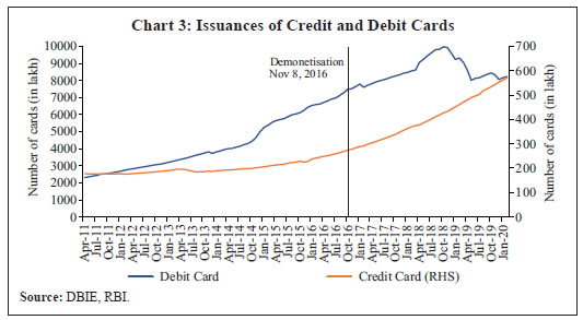
| Table 3: Currency in Circulation – Key Ratios | | (Per cent) | | Ratio | 1971-80 | 1981-90 | 1991-2000 | 2001-10 | 2011-20 | 1971-2020 | | CiC/GDP | 9.3 | 9.4 | 9.9 | 11.9 | 11.3 | 11.3 | | CiC /PFCE | 14.2 | 19.4 | 23.2 | 28.7 | 25.6 | 19.1 | | CiC /M0 | 84.4 | 67.2 | 65.9 | 71.0 | 75.8 | 74.0 | | CiC /M1 | 58.8 | 60.1 | 56.8 | 54.4 | 63.2 | 63.9 | | CiC /M3 | 30.9 | 22.1 | 19.0 | 15.3 | 14.4 | 15.7 | | Source: DBIE, RBI; authors’ calculations. | Annually, the CiC/GDP ratio has increased gradually since the second half of the 1990s (Chart 1). At the same time, there has been (i) a steady increase in the share of the services sector in overall GDP and (ii) lower transaction costs of holding cash (rise in the number of ATMs). After reaching a peak of 12.6 per cent in 2009-10, the CiC/GDP ratio plummeted to 8.7 per cent in 2016-17 after demonetisation. As mentioned earlier, a gradual increase in CiC over the last three years led to an increase in the ratio to 12.0 per cent in 2019-20 (partially facilitated by lower nominal GDP) albeit lower than the peak of 2009-10. III.i Demonetisation As mentioned before, high value currency notes of ₹500 and ₹1,000 denomination amounting to ₹15.4 lakh crore, constituting 86.9 per cent of the then total value of CiC, were demonetised on November 8, 2016 (RBI, 2017). This decision was taken to eliminate corruption, black money, counterfeit currency and terror funding and was guided by the motive of reaping potential benefits. Perceived medium-term gains from demonetisation included (i) greater digitisation; and (ii) greater formalisation of the economy through increased flow of financial savings, which would lead to higher GDP growth, augment tax revenues and improve the overall business environment (ibid.). The decline in CiC after demonetisation was sharp as high value notes were withdrawn while new notes were gradually injected into the system. Between November 4, 2016 and January 6, 2017 (i.e., in the weeks immediately prior to the lowest level of CiC witnessed after demonetisation), total CiC declined by about ₹9 lakh crore. On the first anniversary of demonetisation, a study undertaken by Singh et al. (2017) for the sample period Q3:1998 to Q2:2017 used rolling regressions and found that the income elasticity of currency demand experienced a significant drop to 0.91 in Q2:2017 (post-demonetisation period) from 1.07 in Q2:2014; furthermore, the demonetisation impact was found to be statistically significant. Remonetisation occurred at a rapid pace during 2017-18, wherein CiC reached its pre-demonetisation level by March 9, 2018. As on May 22, 2020, CiC growth at 18.4 per cent (y-o-y) was higher than 14.2 per cent a year ago. As on May 22, 2020, CiC was about 45.2 per cent higher than its pre-demonetisation level. As a proportion of broad money (M3), CiC at 15.2 per cent on May 22, 2020 was also higher than 14.4 per cent immediately prior to demonetisation (on October 28, 2016). III.ii ATMs and Digital Payments The number of cash withdrawal transactions from ATMs has increased significantly since 2014-15 – both through debit and credit cards (Chart 2). Although India is next only to China in terms of cash withdrawals from ATMs, the percentage of cash withdrawals to GDP has remained broadly unchanged at around 17 per cent over the last five years (RBI, 2020). Nevertheless, in terms of both volume and value of cash withdrawals through ATMs, the growth has been slow when compared with digital payment transactions, indicating a shift towards digitisation. This is possibly because the infrastructure for cash withdrawal, i.e., ATMs, has grown at a slow pace of about 4 per cent over the last five years. Monthly data from April 2011 on the number of credit and debit cards issued suggest a significant spurt in debit card issuance from October 2014 through November 2018. In contrast, credit card issuance has increased at a steady pace, especially after demonetisation (Chart 3). The increase in card issuances has facilitated the growth in both online and physical POS terminals-based card payments, resulting in an increase in digital transactions. Commercial banks also issued new cards to comply with the requirement to convert all existing magnetic stripe (magstripe) cards to Europay, Mastercard, and Visa (EMV) chip and Personal Identification Number (PIN) compliant cards by December 31, 2018 and subsequently removed deactivated cards from the system resulting in a drop in the number of active debit cards after November 2018, as mentioned before. This reduction was partly also due to the consolidation of public sector banks. 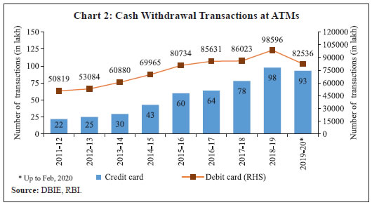
 The volume of total card issuance, which registered a secular increase from October 2014 to a peak of about 10,413 lakh in November 2018, dipped to 8,494 lakh in May 2019 because of the deactivation of some debit cards (Chart 4a). The share of credit cards in total card issuances, however, was less than 10 per cent (ranging from 3.4 to 7.2 per cent) during April 2011 to October 2019. The share of debit cards reached its peak of 96.6 per cent in January 2016 (Chart 4b). Both in terms of value and volume (number of transactions), digital payments have grown rapidly in the last five years (Chart 5). Digital payments comprise both wholesale and retail payments. Wholesale transactions, in the form of real-time gross settlement system (RTGS), are of high value and cannot substitute cash. They are, therefore, not considered in our analysis. For the purpose of this study, retail payments comprising prepaid payment instruments (PPIs), credit cards, debit cards and retail electronic clearing (REC) are more appropriate. REC consists of (i) National Electronic Funds Transfer (NEFT); (ii) Immediate Payment Service (IMPS); and (iii) National Automated Clearing House (NACH). In volume terms, PPI, credit cards, debit cards and REC are broadly of the same size. 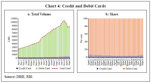 There has been a considerable increase in the number of PPIs comprising mainly mobile wallets and PPI cards with credit and debit cards also reflecting a sharp increase in usage after demonetisation (Chart 6a). The usage remained higher even during the remonetisation phase, although card usage somewhat shrank as cash got replenished in the system. In value terms, REC constitutes 94.1 per cent of digital transactions (Chart 6b). 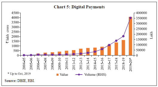 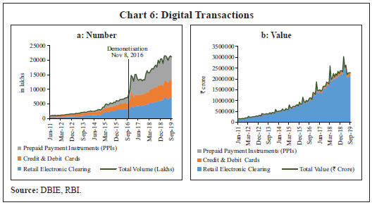 Technological innovation is making digital payments increasingly convenient, instantaneous and ubiquitous. Systems that offer near instant person-to-person retail payments are becoming increasingly available globally. Many payment systems in the country now operate 24 hours a day, seven days a week, thereby alluring customers. The fast payment systems in India such as IMPS and the Unified Payments Interface (UPI) are driving the volume in retail payments. In addition, the availability of NEFT on a 24x7x365 basis (with half-hourly settlements) since December 16, 2019 is likely to propel digital payments in India to a higher growth trajectory. Greater digitalisation of retail transactions and the sharp increase in electronic modes of payments might have resulted in a downward shift in currency demand. Time series forecasts of quarterly CiC movements, both in relation to GDP (CiC/GDP) and in level form, were generated separately using a univariate unobserved components model (UCM)6 based on data from Q1:2001-02 to Q2:2016-17. The forecast of CiC/GDP for the remonetisation period (Q3:2016-17 and beyond) is represented by the dotted line representing the path of CiC/GDP in the absence of demonetisation whereas the thick blue line represents the actual value of CiC/GDP (Chart 7a). This model’s performance was robust for the period prior to demonetisation, tracking the path of actual CiC/GDP ratio fairly accurately (represented by the thick orange line). Based on the model forecast, it is noted that the CiC/GDP ratio could have been higher by 0.9 percentage points in Q3:2018-19 (11.8 per cent instead of the actual 10.9 per cent) in the absence of demonetisation. Thus, the forecast path beyond the demonetisation period can be treated as a counterfactual scenario of the expected path of CiC/GDP in the absence of demonetisation. A similar analysis using the level of CiC (in logarithm) also suggests that CiC would have been significantly higher at the end of Q3:2019- 20 than its actual level in the absence of demonetisation (Chart 7b). 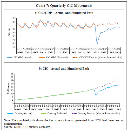 Section IV
Methodology and Data IV.i Weekly Model As mentioned before, forecasting banking system liquidity on a weekly basis is of paramount importance for the effective conduct of liquidity management operations. Accurate forward-looking liquidity assessment is contingent on accurate forecasts of CiC. Consequently, the forecast performance often outweighs the consideration for strong theoretical underpinnings in the weekly model. Moreover, data on variables which are proximate determinants of currency demand in the medium term – viz., income and opportunity cost of holding cash or any of their suitable proxies – are not available at a weekly frequency. Hence, the weekly model for forecasting CiC is based on an atheoretic framework, focusing on time series properties, idiosyncratic factors and other short-term determinants following the available literature (Khatat, 2018). Since CiC is a trending variable exhibiting non-stationarity, the dependent variable in the model is represented as the weekly change in the logarithm of CiC (ΔLCiC). The model controls for (i) persistence; (ii) volatility clustering; (iii) seasonality; (iv) Indian festivals; (v) national and state elections; and (vi) demonetisation as discussed below. (a) Persistence: The dynamic nature of ΔLCiC is modelled by incorporating the lag terms, autoregressive (AR) terms and moving average (MA) terms. (b) Volatility Clustering: In view of high frequency of data on CiC, the possibility of volatility clustering cannot be ruled out; hence, statistical tests are conducted to identify the presence/absence of volatility clustering. Accordingly, we first estimate an ARIMA model for the sample period and test for the heteroscedasticity in residuals using the Breusch-Pagan-Godfrey test. On being found significant, the variance equation is required to be augmented with the ARIMA equation so as to control for the residual heteroscedasticity. Thus, we estimate an autoregressive conditional heteroscedastic (ARCH) model for ΔLCiC. (c) Seasonality: The seasonality is captured using monthly and weekly dummies; eleven dummies have been used to represent the monthly seasonality, with September (middle of the financial year) being the reference period. One month is dropped to avoid the dummy variable trap.7 The weekly seasonality is controlled by using three weekly dummies representing the 2nd, 3rd, and 4th weeks in a month where the 1st week is taken as the reference period. (d) Indian Festivals: In India, consumption usually increases during the festive season which, in turn, leads to an increased demand for currency. Since most of the festivals follow a lunar calendar, these changes are not captured in the seasonal dummies and need to be separately incorporated. The main festivals considered are Diwali, Dussehra, Eid and Ganesha Chaturthi. Usually, currency demand starts rising days before the festival and continues during the festive period; however, subsequently, currency returns (flows back) to the banking system. Accordingly, three dummies are considered separately for each of these festivals to capture the impact of the festive season: pre-festive week, festive week and post-festive week, respectively. (e) Elections: During the sample period (2004-19), four general elections were conducted in India (2004, 2009, 2014 and 2019). Apart from these elections, state elections were also conducted every year in some states as per their respective electoral cycle. Although the national elections have pan-India coverage, the impact of state elections on CiC depends on the number of days on which elections are held and the population size of the states conducting the elections each time. Accordingly, the model covers the general elections of 2004, 2009, 2014 and 2019 and the state elections in 22 major states comprising 95.1 per cent of India’s total population (as per the 2011 Census), viz., Andhra Pradesh, Assam, Bihar, Chhattisgarh, Delhi, Goa, Gujarat, Haryana, Jharkhand, Karnataka, Kerala, Madhya Pradesh, Maharashtra, Punjab, Puducherry, Rajasthan, Sikkim, Tamil Nadu, Tripura, Uttar Pradesh, Uttarakhand, and West Bengal. Furthermore, elections are conducted in several phases in each state. The dates of all phases of national and state elections between 2004 and 2019 are presented in Table 4. 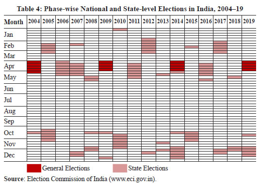 All the information in Table 4 is encapsulated in one indicator of election (Et). Et = 1, if general election is held during week t = Pc/P, if state election/s is/are held during week t = 0 other wise, where Pc represents the total population covered during that phase of the election across all states and P represents pan-India electoral coverage (since electoral details are not available, it is proxied by the population). (f) Demonetisation: As alluded to earlier, CiC fell sharply in November and December of 2016 following demonetisation of high value currency notes, which gradually began to rise subsequently (remonetisation). Accordingly, 20 separate dummy variables are used to represent the demonetisation and remonetisation periods, starting from the second week of November 2016 till end-March 2017. These dummy variables are single period dummies. When single period dummies are used in the regression equation, it is equivalent to removing that particular period from the analysis while estimating the other parameters. Thus, by using single period dummies we have removed the demonetisation and remonetisation periods while estimating the other parameters. These, in addition, will produce zero residuals in those periods, which should not be considered as model accuracy, rather as a technical approach to remove an extraordinarily volatile period from the analysis. The parameters of these dummies, however, can be used to estimate the size of the impact of demonetisation and remonetisation on CiC. Incorporating all these factors, equations (1) and (2) represent the specification of the ARCH model, which is used to forecast CiC at a weekly frequency. The mean equation (1) has 11 dummies for months M1 to M12, except M9, which is the reference month; three weekly dummies (W2 to W4); one dummy each for pre-Dussehra week (Dussehrapre), Dussehra week (Dussehra) and post-Dussehra week (Dussehrapost); one dummy each for pre-Diwali week (Diwalipre), Diwali week (Diwali) and post-Diwali week (Diwalipost); one dummy each for pre-Eid week (Eidpre), Eid week (Eid), and post-Eid week(Eidpost); one dummy each for pre-Ganesha Chaturthi week (Ganeshapre), Ganesha Chaturthi week (Ganesha), and post-Ganesha Chaturthi week(Ganeshapost). We include the variable (E) to capture the impact of both general and state elections. We also include dummy variables for both the demonetisation and remonetisation periods (D1 to D20). In addition, we control for autoregressive and moving average terms. 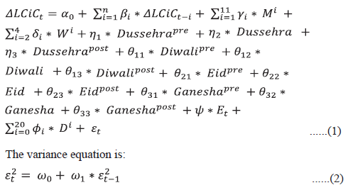 We use weekly data from January 2004 till September 2019, sourced from RBI’s Database on Indian Economy (DBIE).8 IV.ii Monthly Model Incorporating Digital Payments For the monthly CiC model, we use the standard cointegration approach under the time series econometric framework since it has been the conventional workhorse model in estimating short- and long-run relationships among economic variables (Johansen and Juselius, 1990). VECM approach, however, has a shortcoming in that all variables used should be strictly of the same order of integration. The bound testing and ARDL cointegration approaches do not require every variable in the model to necessarily have the same order of integration (Pesaran et al., 2001). The relative merit of this approach is its applicability, irrespective of whether the underlying regressors are purely I(0), purely I(1), or a mixture of both with the condition that none of the series is I(2). Consequently, we formulate a monthly model primarily focusing on the impact of digital payments on CiC following an ARDL bound testing approach. A brief description of the ARDL methodology is given in Appendix D. Following the specification of the demand for currency, long-run cointegration was tested for CiC, nominal income (Y)9 and average deposit rate (ADR), the latter representing the opportunity cost of holding cash. Both Y and CiC are seasonally adjusted and represented in logarithmic form (represented by LY and LCiC). The change in digital transactions in terms of transaction value and number of transactions is alternately used as an explanatory variable in the short-run dynamics along with the error correction term and the other short-run variables. One of the distinctive features of the monthly model is the use of the data on digital payments (component-wise disaggregated data) to forecast CiC. As disaggregated data on digital payments, sourced from DBIE, are available from 2011 onwards (although aggregate data are available from 2004), we restricted the sample period from April 2011 to September 2019 given the surge in digital payments network and infrastructure during the last decade which helps in assessing the impact of its penetration on currency demand. IV.iii Quarterly and Annual Models Similar to the monthly model, the ARDL cointegration approach (Pesaran and Shin 1995, 1999; Pesaran et al., 1996) is used to model the relationship between CiC and other variables for the quarterly and annual models as well. For the quarterly model, data from Q2:1998-99 to Q3:2019-20 encompassing 86 observations have been used, while the annual model is based on data from 1970-71 to 2018-19. The variables used both in the quarterly and annual models are CiC, nominal GDP and average deposit rates of 1-3 years tenor, which are sourced from RBI’s DBIE, National Statistical Office (NSO), Government of India, and State Bank of India. Section V
Results V.i Weekly Model The regression coefficients estimated from equations (1) and (2) are presented in Table 5. The diagnostics of the model are found to be satisfactory. The errors are free from autocorrelation and heteroscedasticity as evident from correlograms of standardised residuals and standardised residual squares along with the ARCH-LM test. The main findings of the model are analysed below. | Table 5: Estimated Regression Coefficients | | Regressor | Coeff. | SE | z | Prob. | Regressor | Coeff. | SE | z | Prob. | | Mean Equation | D6 | 0.060 | 0.021 | 2.810 | 0.005 | | C1 | 0.001 | 0.001 | 1.143 | 0.253 | D7 | 0.059 | 0.027 | 2.227 | 0.026 | | ΔLCiC(-1) | 0.152 | 0.076 | 1.982 | 0.047 | D8 | 0.055 | 0.014 | 3.859 | 0.000 | | ΔLCiC(-2) | -0.019 | 0.047 | -0.409 | 0.682 | D9 | -0.008 | 0.009 | -0.942 | 0.346 | | ΔLCiC(-3) | -0.018 | 0.042 | -0.425 | 0.671 | D10 | 0.082 | 0.008 | 10.491 | 0.000 | | ΔLCiC(-4) | 0.341 | 0.041 | 8.314 | 0.000 | D11 | 0.034 | 0.009 | 3.671 | 0.000 | | ΔLCiC(-5) | 0.038 | 0.039 | 0.992 | 0.321 | D12 | 0.027 | 0.008 | 3.224 | 0.001 | | ΔLCiC(-6) | 0.046 | 0.035 | 1.301 | 0.193 | D13 | 0.041 | 0.009 | 4.638 | 0.000 | | M1 | 0.001 | 0.001 | 0.965 | 0.335 | D14 | 0.018 | 0.007 | 2.513 | 0.012 | | M2 | 0.000 | 0.001 | 0.373 | 0.709 | D15 | 0.011 | 0.018 | 0.605 | 0.545 | | M3 | 0.000 | 0.001 | 0.806 | 0.420 | D16 | 0.016 | 0.014 | 1.154 | 0.248 | | M4 | 0.001 | 0.000 | 6.224 | 0.000 | D17 | 0.010 | 0.016 | 0.631 | 0.528 | | M5 | -0.002 | 0.001 | -2.945 | 0.003 | D18 | 0.005 | 0.012 | 0.441 | 0.659 | | M6 | -0.004 | 0.001 | -5.282 | 0.000 | D19 | 0.009 | 0.013 | 0.705 | 0.481 | | M7 | -0.003 | 0.001 | -4.313 | 0.000 | D20 | 0.010 | 0.012 | 0.883 | 0.377 | | M8 | 0.000 | 0.001 | -0.174 | 0.862 | AR(13) | 0.485 | 0.073 | 6.606 | 0.000 | | M10 | 0.000 | 0.001 | 0.039 | 0.969 | AR(9) | 0.166 | 0.037 | 4.534 | 0.000 | | M11 | -0.002 | 0.001 | -2.696 | 0.007 | AR(4) | 0.106 | 0.090 | 1.180 | 0.238 | | M12 | -0.001 | 0.001 | -0.847 | 0.397 | AR(3) | -0.185 | 0.099 | -1.874 | 0.061 | | W2 | 0.002 | 0.001 | 2.362 | 0.018 | AR(23) | -0.126 | 0.060 | -2.102 | 0.036 | | W3 | 0.001 | 0.001 | 0.605 | 0.545 | AR(1) | 0.002 | 0.110 | 0.018 | 0.986 | | W4 | 0.001 | 0.001 | 0.691 | 0.489 | AR(2) | -0.178 | 0.085 | -2.092 | 0.036 | | Dussehrapre | 0.005 | 0.001 | 4.586 | 0.000 | MA(13) | -0.299 | 0.067 | -4.435 | 0.000 | | Dussehra | 0.006 | 0.001 | 5.869 | 0.000 | MA(3) | 0.344 | 0.118 | 2.913 | 0.004 | | Dussehrapost | -0.003 | 0.001 | -2.270 | 0.023 | MA(4) | -0.314 | 0.116 | -2.710 | 0.007 | | Diwalipre | 0.009 | 0.001 | 11.811 | 0.000 | MA(23) | 0.012 | 0.063 | 0.189 | 0.850 | | Diwali | 0.014 | 0.001 | 12.101 | 0.000 | MA(1) | -0.061 | 0.146 | -0.421 | 0.674 | | Diwalipost | -0.007 | 0.002 | -4.380 | 0.000 | MA(2) | 0.192 | 0.098 | 1.954 | 0.051 | | Eidpre | 0.001 | 0.001 | 0.749 | 0.454 | | Variance Equation | | Eid | 0.001 | 0.001 | 1.211 | 0.226 | | C2 | 0.000 | 0.000 | 13.334 | 0.000 | | εt2(1) | 0.143 | 0.053 | 2.693 | 0.007 | | Eidpost | -0.002 | 0.001 | -2.040 | 0.041 | | E | 0.002 | 0.001 | 2.322 | 0.020 | Diagnostics | | D2 | -0.225 | 0.007 | -30.67 | 0.000 | | D3 | -0.140 | 0.017 | -8.015 | 0.000 | Adjusted R-squared = 0.93 | | D4 | -0.108 | 0.017 | -6.500 | 0.000 | Sum squared residuals = 0.01 | | D5 | -0.076 | 0.018 | -4.211 | 0.000 | Heteroscedasticity Test ARCH-LM p-value = 0.41 | | Note: Coeff. : Coefficient value; SE: Standard Error; z: z-Statistics; Prob.: Probability. | (a) Seasonality: CiC increases in March and April compared to September (reference month), while it declines during May, June and July (Chart 8a). The increase in CiC in March and April can be attributed to the rabi harvest, rice and wheat procurement, marriage season and celebration of Hindu New Year festivals (e.g., Gudhi Padwa, Pongal, Baisakhi, Ugadi) across India. The decline in CiC during May, June and July roughly coincides with the monsoon season. A priori, it is expected that CiC would be higher during the festive season (October to December) compared with other months. As we have explicitly modelled the impact of several festivals separately through festival dummies, the partial regression coefficients of seasonal dummies corresponding to those months are not statistically significant and positive. In fact, these effects were reflected in the weekly dummies corresponding to those festivals. Thus, the seasonal dummies for the festive period (October to December) do not show any significant uptick compared with September after controlling for those effects. While considering intra-month movements, the largest increase in CiC occurs in the second week (Chart 8b). 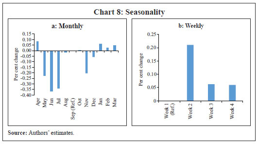
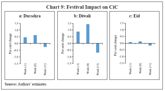 (b) Festivals: Ganesha Chaturthi did not have statistically significant impact on CiC at the national level; hence, this festival was dropped from the final regression equation. CiC increases before and during the festive weeks, part of which returns to the banking system a week later (Chart 9 and Table 5). Among the festivals, Diwali has the largest impact on CiC (Chart 9b). Cumulatively, CiC increases by around 2.2 per cent during Diwali followed by Dussehra (1.1 per cent) and Eid (0.2 per cent). (c) Elections: The regression coefficient corresponding to the election variable was found to be positive and statistically significant. CiC increases by 0.2 per cent in each week (on average) during the period in which general elections are held; thus, CiC is expected to increase cumulatively by 1 per cent if the general election phase is held over a five-week period.10 The estimates also suggest that the impact is larger if there is (i) a larger size of the electorate (general or bigger state elections) and (ii) if the duration of the electoral process is longer. 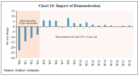 (d) Demonetisation: The estimated regression coefficients of the demonetisation dummies suggest that CiC did fall significantly by about 55 per cent11 during the first four weeks after demonetisation (Chart 10). After remonetisation began, the increase in CiC stock (statistically significant) was from week 4 (W4) to week 12 (W12) when nearly 36.8 per cent CiC got replenished, which increased further to 43 per cent by April 2017. (e) Forecast Performance: The model is used to produce pseudo out-of-sample one week ahead forecasts for 2018 and 2019. A comparison of the fitted and actual values of the percentage changes in CiC suggests that the model can reasonably predict currency movements (Chart 11). The average out-of-sample root mean square error (RMSE) for 2018 and 2019 was found to be 0.33 per cent. V.ii Monthly Model Incorporating Digital Payments The bound testing cointegration test with alternate specifications suggests that LY, LCiC and ADR are not cointegrated, unlike in the quarterly model discussed below (Table 6). After removing ADR, however, LY and LCiC were found to be cointegrated. This is different from the results obtained from the quarterly model on account of the difference in the sample period – a shorter sample for the monthly model (2011-19) and a longer sample for the quarterly model (1997-2019). This could be attributed to the fact that the bank deposit rate may no longer represent the opportunity cost of money with the proliferation of several new financial market products in the more recent period. 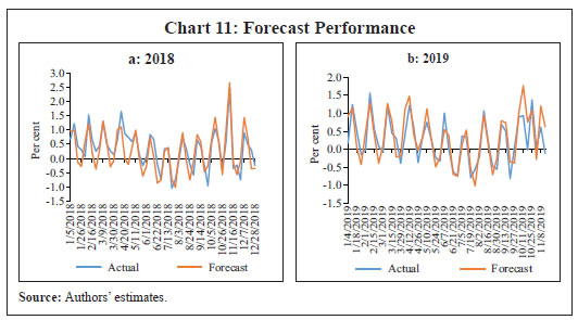 To understand the short-run dynamics, the value and the number of digital transactions are used alternately as additional explanatory variables along with the other short-term variables. The regression results suggest that the long-run coefficient of nominal income is statistically significant and close to unity (Table 7). In the short run, the error correction term is negative and significant. The change in the value of transactions is found to be statistically insignificant; however, the number of transactions is found to be statistically significant and negative (with one period lag) indicating that an increase in the number of digital transactions helps in reducing CiC (Table 7, Regression 2). This suggests that the penetration/coverage of digital transactions can significantly impact CiC demand. | Table 6: Test for Cointegration | | Model with variables | LY, LCiC and ADR | LY and LCiC | | Bound Test | F = 2.486 | F = 5.933 | | Critical Values (5 per cent) | [3.79 4.85 ] | [4.94 5.73] | | Inference | Not Cointegrated | Cointegrated |
| Table 7: Regression Coefficients – Long-run and Short-run | | Regressor | Regression 1 | Regression 2 | | Long-run coefficient of LY | 0.936
(0.00) | 0.909
(0.00) | | Short-run coefficients | | Error correction | -0.067
(0.00) | -0.070
(0.00) | | ΔLog of value of digital transactions | 0.009
(0.75) | -- | | ΔLog of value of digital transactions (-1) | 0.023
(0.40) | -- | | ΔLog of number of digital transactions | -- | -0.027
(0.36) | | ΔLog of number of digital transactions (-1) | -- | -0.052
(0.07) | | Diagnostics | | LM test for autocorrelation (p-value) | 0.02 | 0.06 | | BP test for heteroscedasticity (p-value) | 0.02 | 0.06 | | Note: Figures in parentheses are probability values. | A disaggregated analysis with number of transactions in REC, Cards and PPI was undertaken to measure the impact of each instrument on CiC. The findings suggest that the long-run coefficients of nominal income are statistically significant and close to unity in all specifications (Table 8). Short-run dynamics indicate that the number of card transactions significantly moderates CiC expansion. V.iii Quarterly Model The correlation matrix reveals that there is a strong and statistically significant positive correlation between LY and LCiC, as expected (Table 9). Furthermore, in accordance with the theory, there is a negative and statistically significant correlation between ADR and LCiC. Table 8: Regression Coefficients – Long-run and Short-run Coefficients
(Alternative modes of payment) | | Regressor | Regression 1 | Regression 2 | Regression 3 | | Long-run coefficient of LY | 0.922
(0.00) | 0.916
(0.00) | 0.922
(0.00) | | Short-run coefficients | | Error correction | -0.068
(0.00) | -0.060
(0.00) | -0.068
(0.00) | | ΔLog of number of PPI transactions | 0.000
(0.99) | -- | -- | | ΔLog of number of PPI transactions (-1) | 0.001
(0.86) | -- | -- | | ΔLog of number of card transactions | -- | -0.072
(0.07) | -- | | ΔLog of number of card transactions (-1) | -- | -0.131
(0.00) | -- | | ΔLog of number of REC transactions | -- | -- | 0.008
(0.68) | | ΔLog of number of REC transactions (-1) | -- | -- | -0.004
(0.83) | | Diagnostics | | LM test for autocorrelation (p-value) | 0.01 | 0.25 | 0.04 | | BP test for heteroscedasticity (p-value) | 0.02 | 0.05 | 0.02 | | Note: Figures in parentheses are probability values. | As mentioned before, the ARDL technique (Pesaran and Shin, 1995, 1999; Pesaran et al., 1996) is used to model the relationship between LCiC and other variables for the quarterly and annual model. The augmented Dickey-Fuller (ADF) and Phillips-Perron (PP) tests are employed to test the stationarity properties of the variables under consideration. The unit root tests in the form of ADF and PP indicate that the variables under consideration are either I(1) or I(0), but not I(2), as is appropriate for estimating an ARDL model12 (Table 10). | Table 9: Correlation Matrix | | Correlation | LCiC | | LY | 0.99* | | ADR | -0.23* | | Note: * significant at 1 per cent level. |
| Table 10: ADF and PP Unit Root Tests | | Variable | Level | First Difference | | ADF | PP | ADF | PP | | LCiC | -0.673 | -0.997 | -9.9293* | -18.280* | | LY | -0.022 | -0.869 | -3.103* | -13.847* | | ADR | -2.980* | -2.195 | - | -8.030* | Note: * denotes significance at 1 per cent. The constant and time trends are included in level, but the time trend is removed in the first difference equation. The optimal lag order is selected based on SIC in the ADF test equation.
- = Not applicable. | The F-statistic and critical values under the bounds test are presented in Table 11. The cointegration test applied on the unrestricted model is an F-test on the hypothesis that the coefficients of the lagged level variables are jointly equal to zero. The F-statistic for the joint significance of the parameters of the lagged level variables is found to be 22.90, which exceeds the upper bound critical value. The results, therefore, reveal statistically significant evidence in favour of the existence of a long-run cointegrating relationship between the variables under consideration. The long-run ARDL cointegration test shows statistically significant unitary income elasticity of currency demand (Table 12). The expected inverse relationship between average deposit rate and CiC, however, is statistically insignificant. The error correction model (ECM) under the ARDL approach is estimated to examine the short-run dynamics of the relationship between dependent and independent variables to estimate the persistence of short-run shocks and the speed of adjustment for the return to equilibrium. The estimated error correction term is negative and significant, thereby indicating that the system reverts to equilibrium regardless of any short-run shock to the system (Table 13). The adjustment to the short-run shock, however, is quite slow – only 4 per cent of deviation because of any short-run shock gets corrected in a quarter. | Table 11: Bounds Test for Cointegration | | F-statistic | 99% lower bound | 99% upper bound | Outcome | | 22.90 | 4.13 | 5.00 | cointegration |
| Table 12: Long-run ARDL Cointegration Model (2, 1, 2)# | | Dependent variable: LCiC | | Regressor | Coefficient | t-Statistics | | LY | 1.048 | 17.87* | | ADR | -5.845 | -1.29 | | C | 0.625 | 0.45 | # Lag length is selected using Akaike Information Criteria (AIC).
Note: * denotes significance at 1 per cent. | We infer from the estimated short-run relationship that the change in nominal GDP influences change in CiC positively and the change in average deposit rate has a negative impact on the change in CiC – both these relationships being statistically significant. In the short run, the impact of the average deposit rate is higher: (i) one percentage point increase in deposit rate leads to a 0.34 per cent decline in CiC over a period of two quarters, while (ii) one percentage point increase in nominal GDP leads to a 0.13 per cent increase in CiC in the same quarter. Furthermore, the model is robust on the basis of all diagnostic tests – no residual serial autocorrelation and heteroscedasticity, and parameter stability – as depicted in the lower panel of Table 13. We also conducted the same empirical exercise using ARDL methodology with annual data, the details of which are given in Appendix A. The results are broadly in line with the findings obtained in the case of the quarterly model. In terms of the degree of impact, CiC has the same unitary elasticity with respect to nominal GDP in the long run as in the quarterly model (Appendix A, Table A.4). The impact of the deposit rate, however, is qualitatively different – it is statistically significant in the annual model, while not so in the quarterly model. The longer time horizon of the annual model may have contributed to this divergence in results. The quarterly data represent the recent one-and-a-half decades when the economy witnessed proliferation of several alternative financial instruments, while the annual data represent a longer time period, the earlier half of which was characterised by limited avenues for financial savings other than bank deposits. Financial market development and other avenues for savings available in the more recent period might have reduced the role of bank deposit rates as a proxy for the opportunity cost of currency in the quarterly model compared to the annual model. Short-run results, as expected, are stronger in the annual model with income elasticity being higher than in the quarterly model (Appendix A, Table A.5). | Table 13: ARDL Cointegration Short-run Error Correction Model13 | | Dependent variable: ΔLCiC | | Regressor | Coefficient | t-Statistics | | ΔLCiC(-1) | -0.164 | -1.53 | | ΔLY | 0.130 | 2.50* | | ΔADR | -1.202 | -2.49** | | ΔADR(-1) | 0.861 | 1.80*** | | Q2DUM | -0.062 | -10.25* | | Q3DUM | -0.018 | -1.79*** | | Q4DUM | -0.010 | -1.44 | | Q32017DUM | -0.662 | -40.70* | | Q42017DUM | 0.174 | 2.32* | | Q12018DUM | 0.122 | 3.39* | | Q22008DUM | 0.050 | 2.75** | | Error Correction (-1) | -0.040 | -9.77* | | Diagnostic tests | | Adjusted R2: | 0.98 | | DW statistics: | 1.83 | | LM serial correlation F-test (p-value): | 0.49 | | Breusch-Pagan-Godfrey heteroscedasticity Test F-test (p-value): | 0.34 | | CUSUM test: | Stable | | CUSUM of squares test: | Stable | | Note: *, ** and *** denote significance at 1 per cent, 5 per cent and 10 per cent, respectively. | Section VI
Concluding Observations In view of the importance of currency movements for implementation of monetary policy, this study draws on the existing literature to construct a menu of models for analysing and forecasting currency demand using a variety of time series and econometric techniques. The objective of the study was to develop a weekly currency forecasting model and analyse the determinants of currency demand with lower frequency data. Several important findings emerge from the study. Digital payments are playing an increasingly important role in changing the payment habits of economic agents. The increased use of digital payments in the recent period has reduced the demand for currency, which has important ramifications for currency demand in the future. Moreover, policy-induced measures such as demonetisation have also brought about a downward shift in the trend component of currency which would have been much higher in the absence of demonetisation. The key findings of the study from the weekly model are: (i) currency demand is higher in March and April and lower during the monsoon season; (ii) intra-month movements indicate a surge in currency demand in the second week of the month; (iii) demand for currency is also high during the festive season, especially during Diwali; and (iv) currency demand increases cumulatively by about 1 per cent during general elections when the election phase spans five weeks; the impact of elections on currency is higher if there are national or bigger state elections and if the duration of the electoral process is longer. The monthly model incorporating digital payments suggests that (i) long-run income elasticity of currency demand is close to unity; and (ii) an increase in the number of digital (credit and debit card) transactions dampens currency demand in the short run. Findings from the quarterly model indicate that (i) in the long-run, income elasticity of currency demand is unity while the interest rate is not found to have any significant impact; and (ii) in the short run, however, both impact currency demand. Finally, the annual model suggests that: (i) currency has unitary income elasticity and the interest rate also impacts currency demand in the long run; and (ii) income elasticity in the annual model is higher than that in the quarterly model in the short-run. There are several important policy implications that emerge from the findings. First, income continues to be a key determinant of currency demand and income elasticity of currency demand is unity in all the models across the time horizon. Therefore, currency demand in the foreseeable future is expected to grow broadly at the same rate as nominal income, which serves as an important guide for policy making. Second, it is found that currency will expand relatively at a faster (slower) pace in a low (high) interest rate environment when the opportunity cost of holding money is low (high), given the inverse relationship between currency demand and the interest rate. Third, since digital transactions (especially credit and debit cards) have a dampening impact on currency demand, there is a need to sustain the current thrust on digital transactions if currency growth is to be further moderated. Going ahead, there is a scope to further extend the study in many dimensions. The availability of more granular-level data on digital payments over a longer time horizon would enable improved modelling of currency demand at the quarterly and annual frequencies. Increasing sophistication of financial markets would imply the availability of several alternative investment avenues for economic agents instead of relying solely on bank deposits. As a result, financial market returns from several alternative instruments can also be tested as proxies for the opportunity cost of holding cash rather than just deposit interest rates. Survey-based data on the public’s preferences with regard to payment habits could also be a proxy for any behavioural shift in currency demand. Furthermore, purely statistical techniques such as a neural network model can be used for currency forecasting at higher frequency (daily data) for comparison with model-based forecasts. All of these issues, however, merit an in-depth analysis and could be the agenda for future research.
References Arango, C., Huynh, K. P., & Sabetti, L. (2015). Consumer payment choice: Merchant card acceptance versus pricing incentives. Journal of Banking & Finance, 55, 130-141. Arango-Arango, C. A., Bouhdaoui, Y., Bounie, D., Eschelbach, M., & Hernandez, L. (2018). Cash remains top-of-wallet! International evidence from payment diaries. Economic Modelling, 69, 38-48. Basnet, H. C., & Donou-Adonsou, F. (2016). Internet, consumer spending, and credit card balance: Evidence from US consumers. Review of Financial Economics, 30, 11-22. Baum, C. & Hristakeva, S. (2001). DENTON: Stata module to interpolate a flow or stock series from low-frequency totals via proportional Denton method, Statistical Software Components S422501, Boston College Department of Economics, revised 17 July, 2014. Baumol, W. J. (1952). The transactions demand for cash: An inventory-theoretic approach. Quarterly Journal of Economics, 66(4), 545-556. Bhattacharya, K., & Joshi, H. (2000). Modeling currency in circulation in India. Applied Economic Letters, 8(9), 585-592. —. (2002). An Almon approximation of the day of the month effect in currency in circulation. Indian Economic Review, 36(2), 163-174. Bhattacharya, K., & S. K. Singh (2016). Impact of payment technology on seasonality of currency in circulation: Evidence from the USA and India. Journal of Quantitative Economics, 14(1), 117-136. Bech, M. L., Faruqui, U., Ougaard, F., & Picillo, C. (2018). Payments are a-changin’ but cash still rules. BIS Quarterly Review, March. Cassino, V., Misich, P., & Barry, J. (1997). Forecasting the demand for currency. Reserve Bank of New Zealand Bulletin, 60. https://ideas.repec.org/a/nzb/nzbbul/march19973.html Chaudhari, D. R., Dhal, S., & Adki, S. M. (2020). Payment system innovation and currency demand in India: Some applied perspective. RBI Occasional Papers, 40(20), 33-58. Columba, F. (2009). Narrow money and transaction technology: New disaggregated evidence. Journal of Economics and Business, 61(4), 312-325. Dotsey, M. (1988). The demand for currency in the United States. Journal of Money, Credit and Banking, 20(1), 22-40. http://doi.org/10.2307/1992665 Durgun, O., & Timur, M. C. (2015). The effects of electronic payments on monetary policies and central banks. Procedia-Social and Behavioral Sciences, 195, 680-685. Fischer, A. M. (2007). Measuring income elasticity for Swiss money demand: What do the cantons say about financial innovation? European Economic Review, 51(7), 1641-1660. Fujiki, H., & Tanaka, M. (2014). Currency demand, new technology, and adoption of electronic money: Micro evidence from Japan. Economic Letters, 125, 5-8. Galbraith, J. W., & Tkacz, G. (2018). Nowcasting with payments system data. International Journal of Forecasting, 34(2), 366-376. Harvey, A., Koopman, S. J., & Riani, M. (1997). The modeling and seasonal adjustment of weekly observations. Journal of Business & Economic Statistics, 15(3), 354-368. Hazra, D. (2017). Monetary policy and alternative means of payment. The Quarterly Review of Economics and Finance, 65, 378-387. Hlaváček, M., Čada, J., & Hakl, F. (2005). The application of structured feedforward neural networks to the modelling of the daily series of currency in circulation. In L. Wang, K. Chen, Y.S. Ong (Eds.), Advances in natural computation. Lecture Notes in Computer Science, vol. 3610. Springer. http://link.springer.com/chapter/10.1007/11539087_163 Jadhav, N. (1994). Monetary economics for India. Macmillan India Ltd, New Delhi. Johansen, S., & Juselius, K. (1990). Maximum likelihood estimation and inference on cointegration - with applications to the demand for money. Oxford Bulletin of Economics and Statistics, 52(2), 169-210. Johnson, N. L., Kotz, S., and Balakrishnan, N. (1994). Continuous univariate distributions (2nd ed., Vol. I). New York: Wiley. Kahn, C. M., & Roberds, W. (2009). Why pay? An introduction to payments economics. Journal of Financial Intermediation, 18(1), 1-23. Karni, Edi, (1973). The transactions demand for cash: Incorporation of the value of time into the inventory approach. Journal of Political Economy, 81(5), 1216-1225. Khatat, M. E. (2018). Monetary policy and models of currency demand. IMF Working Paper WP/18/28. Koziński, W., & Świst, T. (2015). Short-term currency in circulation forecasting for monetary policy purposes: The case of Poland. Financial Internet Quarterly eFinanse, 11(1). Kulatunge, S. (2019). Modeling and forecasting currency demand in Sri Lanka: An empirical study. International Journal of Business and Social Science, 10(6), 62-73. Kumar, S. (2011). Financial reforms and money demand: Evidence from 20 developing countries. Economic Systems, 35(3), 323-334. Li, C. (2007). Essays on the inventory theory of money demand. https://circle.ubc.ca/handle/2429/417 Lee, M. (2014). Constrained or unconstrained price for debit card payment? Journal of Macroeconomics, 41, 53-65. Lotz, S., & Zhang, C. (2016). Money and credit as means of payment: A new monetarist approach. Journal of Economic Theory, 164, 68-100. Maiti, S. S. (2017). From cash to non-cash and cheque to digital: The unfolding revolution in India’s payment systems, Mint Street Memo No. 07. https://www.rbi.org.in/Scripts/MSM_Mintstreetmemos7.aspx Miller, M. H., & Orr, D. (1966). A model of the demand for money by firms. Quarterly Journal of Economics, 80(3), 413-435. Nachane, D. M., Chakraborty, A. B., Mitra, A. K., & Bordoloi, S. (2013). Modelling currency demand in India: An empirical study. DRG Study No. 39, Reserve Bank of India. Oyelami, L. O., & Yinusa, D. O. (2013). Alternative payment systems implication for currency demand and monetary policy in developing economy: A case study of Nigeria. International Journal of Humanities and Social Science, 3(20), 253-260. Palanivel, T., & Klein, L. R. (1999). An econometric model for India with emphasis on the monetary sector. The Developing Economies, 37(3), 275-327. http://doi.org/10.1111/j.1746-1049.1999.tb00235.x Pesaran, M. H. and Pesaran, B. (1997). Working with Microfit 4.0: Interactive Econometric Analysis, Oxford University Press, Oxford. Pesaran, M. H., & Shin, Y. (1995). Autoregressive distributed lag modelling approach to cointegration analysis, DAE Working Paper Series No. 9514, Department of Applied Economics, University of Cambridge. — (1999). Autoregressive distributed lag modelling approach to cointegration analysis. In S. Storm (Ed.), Econometrics and economic theory in the 20th century: The Ragnar Frisch Centennial Symposium. Cambridge: Cambridge University Press. Pesaran, M. H., Shin, Y., & Smith, R. J. (1996). Testing the existence of a long-run relationship. DAE Working Paper Series No. 9622, Department of Applied Economics, University of Cambridge. —. (2001). Bounds testing approaches to the analysis of level relationships. Journal of Applied Econometrics, 16(3), 289-326. Reddy, S., & Kumarasamy, D. (2017). Impact of credit cards and debit cards on currency demand and seigniorage. Academy of Accounting and Financial Studies Journal, 21(3), 1-15. Reserve Bank of India (RBI) (2002). A short term liquidity forecasting model for India, June. https://rbidocs.rbi.org.in/rdocs//PublicationReport/Pdfs/30016.pdf — (2017). Macroeconomic impact of demonetisation: A preliminary assessment, March. https://m.rbi.org.in/scripts/OccasionalPublications.aspx?head=Macroeconomic%20Impact%20 of%20Demonetisation Singh, B., Behera, H., Raut, D. & Roy, I. (2017). Impact of demonetisation on the financial sector. RBI Bulletin, November. Stavins, J. (2018). Consumer preferences for payment methods: Role of discounts and surcharges. Journal of Banking & Finance, 94, 35-53. Tobin, J. (1956). The interest-elasticity of transactions demand for cash. Review of Economics and Statistics, 38(3), 241-47.
Appendix A: Annual Model | Table A.1: Correlation Matrix | | Correlation | LCiC | | LY | 0.99* | | ADR | -0.07 | | Note: * denotes significance at 1 per cent. |
| Table A.2: ADF and PP Unit Root Tests | | Regressor | Level | First Difference | | ADF | PP | ADF | PP | | LCiC | -0.078 | -0.059 | -8.699* | -8.699* | | LY | -0.694 | -0.134 | -4.712* | -4.781* | | ADR | -2.022* | -2.156 | - | -5.689* | Note: * denotes significance at 1 per cent. The constant and time trends are included in level, but the time trend is removed in first difference equations. The optimal lag order is selected based on SIC in the ADF test equation.
- = Not applicable. |
| Table A.3: Bounds Test for Cointegration | | F-statistic | 99% lower bound | 99% upper bound | Outcome | | 21.16 | 4.13 | 5.00 | Cointegration |
| Table A.4: The Long-run ARDL Cointegration Model (2, 1, 1)# | | Dependent variable: LCiC | | Regressor | Coefficient | t-Statistics | | LY | 1.066 | 238.04* | | ADR | -2.465 | -6.044* | | C | -2.690 | -45.49* | # Lag length is selected using Akaike Information Criteria (AIC).
Note: * denotes significance at 1 per cent. |
| Table A.5: ARDL Cointegration Short-run Error-correction Model14 | | Dependent variable: ΔLCiC | | Regressor | Coefficient | t-Statistics | | ΔLiC(-1) | -0.433 | -4.661* | | ΔLY | 1.571 | 15.01* | | ΔADR | -0.765 | -1.62 | | DEMONDUM | -0.307 | -9.18* | | 1972DUM | 0.110 | 3.04* | | 1975DUM | -0.104 | -2.86* | | 2008DUM | 0.084 | 2.23* | | Error Correction (-1) | -0.826 | -9.58* | | Diagnostic tests | | Adjusted R2: | 0.76 | | DW statistics: | 1.89 | | LM serial correlation F-test (p-value): | 0.84 | | Breusch-Pagan-Godfrey heteroscedasticity Test F-test (p-value): | 0.24 | | CUSUM test: | Stable | | CUSUM of squares test: | Stable | | Note: * denotes significance at 1 per cent. |
Appendix B
Appendix C
Appendix D: Multivariate ARDL Method The ARDL approach in this paper consists of estimating the following equation: We start by conducting a bounds test for the null hypothesis of no cointegration. The calculated F-statistic is compared with the critical value tabulated by Pesaran and Pesaran (1997), and Pesaran et al. (2001). If the test statistic exceeds the upper critical value, the null hypothesis of a no long-run relationship can be rejected regardless of whether the underlying order of integration of the variables is 0 or 1. Similarly, if the test statistic falls below a lower critical value, the null hypothesis is not rejected. However, if the test statistic falls between these two bounds, the result is inconclusive. When the order of integration of the variables is known and all the variables are I(1), the decision is made based on the upper bound. Similarly, if all the variables are I(0), then the decision is made based on the lower bound. The ARDL method estimates (p+1)k number of regressions in order to obtain the optimal lag length for each variable, where p is the maximum number of lags to be used and k is the number of variables in the equation. The orders of lags in the ARDL model are selected by the Akaike Information Criterion (AIC), before the selected model is estimated by ordinary least squares (OLS). In the second step, if there is evidence of a long-run relationship (cointegration) among the variables, the following long-run model is estimated: After ascertaining the evidence of a long-run relationship, the next step involves the estimation of the ECM, which indicates the speed of adjustment back to long-run equilibrium after a short-term disturbance. The standard ECM involves estimating the following equation.
|